A Registration Method for ULS-MLS Data in High-Canopy-Density Forests Based on Feature Deviation Metric

Highlights

What are the main findings?

• Currently, the registration of ULS (Unmanned Laser Scanning) and MLS (Mobile Laser Scanning) point clouds in high-canopy-density forests faces challenges such as significant differences in point cloud structure, uneven density, and limited overlap areas, making it difficult to achieve accurate registration.
• Our method achieves high-precision ULS-MLS registration in stratified mixed tropical forests with an average canopy density of 0.93 and pure forest plots in northern China with an average canopy density of 0.75.

What is the implication of the main finding?

• We proposed a solution to address registration obstruction from structural complexity and ULS-MLS discrepancies in dense forests.
• We developed a new feature extraction and correspondence relationship construction methodology for coarse registration.

Abstract

The integration of unmanned aerial vehicle-based laser scanning (ULS) and mobile laser scanning (MLS) enables the detection of forest three-dimensional structure in high-density canopy areas and has become an important tool for monitoring and managing forest ecosystems. However, MLS faces difficulties in positioning due to canopy occlusion, making integration challenging. Due to the variations in observation platforms, ULS and MLS point clouds exhibit significant structural discrepancies and limited overlapping areas, necessitating effective methods for feature extraction and correspondence establishment between these features to achieve high-precision registration and integration. Therefore, we propose a registration algorithm that introduces a Feature Deviation Metric to enable feature extraction and correspondence construction for forest point clouds in complex regional environments. The algorithm first extracts surface point clouds using the hidden point algorithm. Then, it applies the proposed dual-threshold method to cluster individual tree features in ULS, using cylindrical detection to construct a Feature Deviation Metric from the feature points and surface point clouds. Finally, an optimization algorithm is employed to match the optimal Feature Deviation Metric for registration. Experiments were conducted in 8 stratified mixed tropical rainforest plots with complex mixed-species canopies in Malaysia and 6 structurally simple, high-canopy-density pure forest plots in anorthern China. Our algorithm achieved an average RMSE of 0.17 m in eight tropical rainforest plots with an average canopy density of 0.93, and an RMSE of 0.05 m in six northern forest plots in China with an average canopy density of 0.75, demonstrating high registration capability. Additionally, we also conducted comparative and adaptability analyses, and the results indicate that the proposed model exhibits high accuracy, efficiency, and stability in high-canopy-density forest areas. Moreover, it shows promise for high-precision ULS-MLS registration in a wider range of forest types in the future.

1. Introduction

LiDAR has emerged as a powerful active remote sensing technology for capturing forest 3D structural attributes [1], providing critical support for ecological evaluation, sustainable resource management, and carbon accounting [2,3]. LiDAR sensors can be mounted on various platforms to monitor forests, acquiring diverse and rich laser point cloud information of targets [4]. Among these, unmanned aerial vehicle-based laser scanning (ULS) and mobile laser scanning (MLS) are currently the two primary forms of LiDAR applications in forestry [5]. ULS, mounted on drones, can accurately capture upper canopy information with its top-down perspective across larger areas. However, in densely canopied areas, ULS is less effective at obtaining information about internal forest structures. Research by Terryn et al. found that effective pulses penetrating the canopy often account for less than 10% [6]. MLS, with its bottom-up perspective, employs ground-based sensors to scan the plot-scale forest structures. However, MLS does not always sample the whole canopy due to occlusion effects, particularly in high-density forests [7]. In general, both ULS and MLS suffer from significant occlusions when used independently, especially in high-density tropical and subtropical forests. As a result, integrating ULS and MLS data is a critical preprocessing step to mitigate occlusion effects [8]. Accurate registration, which aligns ULS and MLS point clouds within a unified coordinate system, is essential for effective data integration [9].

Although significant progress has been made in laser point cloud registration technology for urban building research [10], studies on ULS and MLS (or ground-based LiDAR) registration in forest research remain relatively limited [11]. In forest point cloud registration, scholars typically combine feature-based coarse registration with optimization-based fine registration. The coarse approach extracts and matches feature elements (points, lines, and planes) to establish correspondences and estimate the initial transformation between point clouds [12].

For feature extraction in forest coarse registration, some researchers have used point cloud histogram features for registration, employing the Fast Point Feature Histogram (FPFH) algorithm for coarse registration of ULS and MLS point clouds in coniferous forests in northern China [13]. Although this method provides a statistical approach to forest registration, it somewhat lacks the effective utilization of geometric features. Some researchers have noted the similarities between ULS and ground-based LiDAR point clouds in the canopy and proposed registration methods based on the canopy [14]. For example, Shao et al. projected the forest onto a binary plane and used the canopy outline to identify corner points for registration. They conducted experiments in coniferous forests with an average canopy density of 0.76, achieving an average RMSE of 0.11 m [15]. This method can quickly identify effective feature points and achieve high-precision registration, making it suitable for forests with distinct forest gap features. Fekry et al. [16] used HDBSCAN canopy clustering and topological persistence to extract key points, enabling automatic UAV LiDAR strip registration with average residuals of 0.3–0.4 m, outperforming traditional methods. Compared to the tree crown canopy, some scholars focus on individual tree features in forest registration. Ref. [17] introduced a UAV-based registration method using Local Maximum (LM) tree apex detection and Singular Value Decomposition (SVD), which achieved a residual error of 0.43 m in coniferous forests with 76% canopy cover. While this approach overcomes limitations in canopy penetration, it may struggle in broadleaf forests due to the indistinct nature of crown maxima.

When it comes to establishing correspondences, some scholars use random sample consensus (RANSAC) for forest point cloud registration [18]. However, the RANSAC algorithm generates correspondences via random sampling and inlier validation but struggles in dense forests due to structural/density discrepancies between ULS and MLS point clouds caused by severe occlusion, limiting valid inliers. Chen et al. [8] used Fast Global Registration (FGR) to register hierarchical point clouds, achieving high accuracy. However, in dense canopy point clouds, the FGR algorithm employs FPFH descriptors and bidirectional geometric verification for matching, yet complex canopy structures with weakened textures and repetitive branching patterns reduce feature distinctiveness, causing ambiguous matches in geometrically similar regions. Yiliu Tan’s algorithm significantly enhances the accuracy of forest point cloud registration through tree position network matching and entropy-optimized structural feature selection [19]. However, in forests characterized by high canopy density and dense undergrowth obstruction, gaps in the point clouds can still lead to the failure of structural feature extraction.

For fine registration, the optimization-based registration methods are widely adopted by scholars to further optimize the results of coarse registration. The Iterative Closest Point (ICP) algorithm, a classic local optimization method, has been widely employed for fine registration. For example, Zhang et al. [13] and Shao et al. [15] successfully applied the ICP algorithm to refine the alignment of forest point clouds.

In general, researchers have proposed various algorithms for feature extraction and registration of ULS and MLS point clouds in forests. Although these algorithms achieve high accuracy in some forests, they perform poorly in dense tropical rainforests, where limited canopy penetration causes significant structural discrepancies between ULS and MLS [20]. Effective point cloud registration relies on robust feature extraction and accurate correspondence establishment [21]. In forest environments, these tasks are hindered by canopy complexity, occlusions, and geometric heterogeneity, including point density variations, inconsistent 3D distributions, limited overlapping features, and large, multi-platform data volumes [11].

To overcome the above challenges and achieve efficient and effective registration, this paper proposes an automatic method to identify sufficient correspondences between ULS and MLS datasets by establishing the deviation relationships between individual tree features derived from ULS and surface point cloud features derived from MLS. This process consists of two stages: ① An individual tree method is used to detect overlapping regions and homologous features, enabling effective noise reduction and complexity control. ② A Feature Deviation Metric strategy is employed to model deviation relationships between corresponding features, where variance constraints enhance robustness by supporting multi-point matching and global spatial evaluation. To evaluate the performance of our proposed method, we conducted experiments in a high-canopy-density tropical rainforest in Malaysia (a complex mixed forest) and in simpler high-canopy-density forests in northern China. The results show that our method not only achieves high accuracy in ULS and MLS registration for high-canopy-density forests but also exhibits a certain level of adaptability.

2. Materials

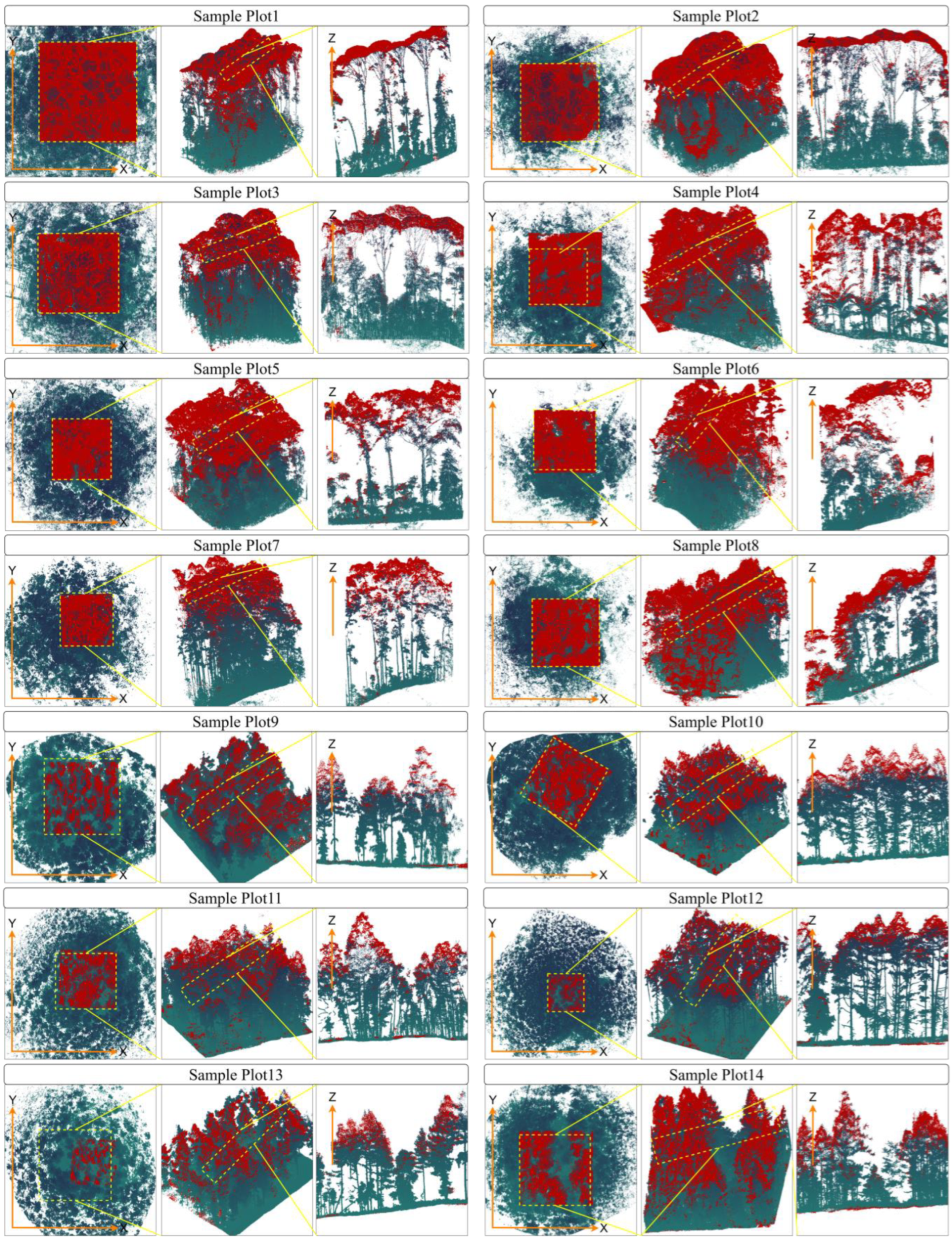
In this study, ULS and MLS data were collected from 14 plots located around the Forest Research Institute Malaysia (8 plots) and Genhe (6 plots), China. Figure 1a displays the spatial distribution of 14 plots.

The study area of Malaysia is located near the southwestern region of Peninsular Malaysia (Forest Research Institute Malaysia), with a longitude range of 101°36′E to 101°39′E and a latitude range of 3°13′N to 3°15′N. The area is characterized by a tropical rainforest climate [22]. The 8 plots in this area are composed of mixed multi-layered forests dominated by species such as Dipterocarpus baudii, Neobalanocarpus heimii, Palaquium gutta, Scorodocarpus borneensis, Shorea bracteolata, and Shorea leprosula [23]. The forest here is a plantation established in the 1920s, containing over a hundred species of both indigenous and exotic plants. Both ULS data and MLS data in the 8 plots were collected from October to December 2023.

The north China study area is located in the Greater Khingan Mountains region of China (GenHe, China), with a longitudinal range from 121°07′04.49″E to 122°01′42.07″E and a latitudinal range from 50°35′57.05″N to 51°44′30.34″N. The climate in this region is classified as a cold temperate humid forest climate. The 6 plots in this area are relatively homogeneous in tree species composition, with Betula platyphylla and Larix gmelinii being the dominant species. Both ULS data and MLS data in the 6 plots were collected from August 2024.

The ULS data were acquired using a Velodyne Ultra Puck LiDAR system, which was mounted on a DJI M200. The UAV platform was equipped with RTK for obtaining positioning information. The coordinates of ULS are in absolute coordinates under the WGS84 coordinate system. The LiDAR scanner used for MLS is the H300 (or H120) laser scanner of GreenValley International, Beijing, China. The coordinates of MLS point clouds are relative coordinates with the plot center as the measurement origin, aligned with the z-axis direction, coinciding with the center of gravity.

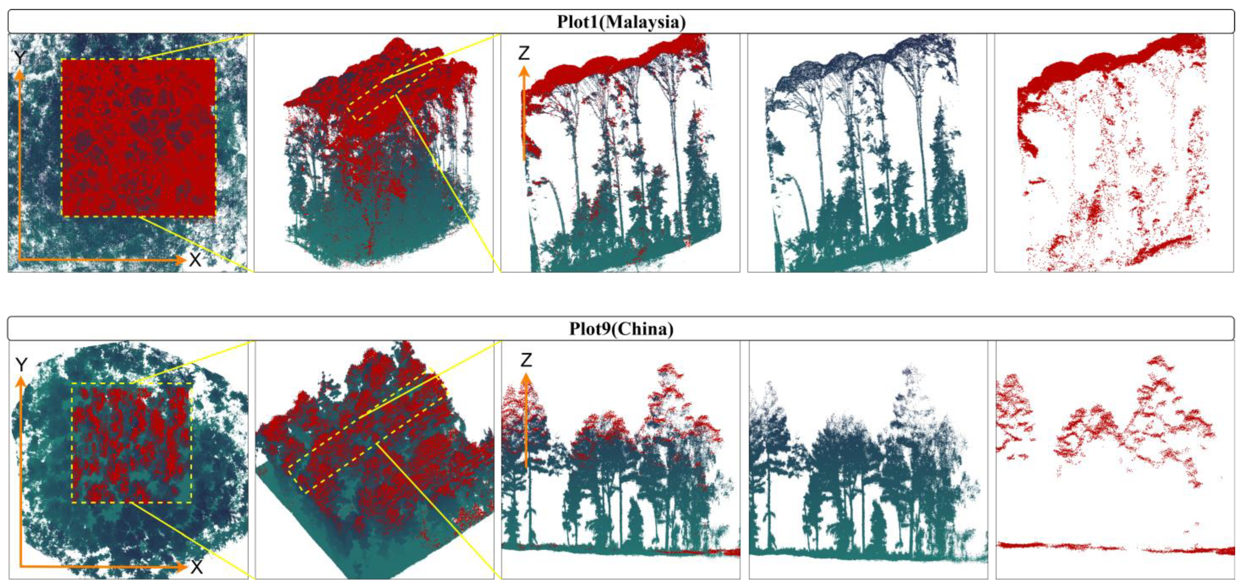
Figure 1b presents a schematic illustration of the MLS and UML point clouds over Plot 1. Visually, it demonstrates that the canopy density in this plot is extremely high. Figure 1c depicts the vertical density variation in point clouds at different heights between ULS and MLS over Plot 1. Specifically, in regions where the height from the ground exceeds 116 m, the point cloud data are predominantly acquired by ULS, whereas below 116 m, MLS is the primary data acquisition method. An overview of the scanned point clouds is provided in

Table 1. Summary of scanned plots.

Plot	Dimension of LiDAR Points (x × y, m)		Date	Tree Species Types	Slope (°)	Canopy Density (0~1)
	ULS	MLS
1	88 × 59	155 × 160	October 2023	Stratified mixed forest	17	0.97
2	75 × 75	145 × 156	November 2023	Stratified mixed forest	6	0.96
3	82 × 70	165 × 157	October 2023	Stratified mixed forest	7	0.98
4	70 × 71	162 × 159	December2023	Stratified mixed forest	18	0.88
5	78 × 74	175 × 157	November 2023	Stratified mixed forest	1	0.94
6	88 × 80	152 × 155	December 2023	Stratified mixed forest	22	0.86
7	68 × 63	152 × 157	December 2023	Stratified mixed forest	15	0.95
8	87 × 68	148 × 164	December 2023	Stratified mixed forest	23	0.90
9	25 × 25	54 × 58	August 2024	Larix gmelinii	5	0.84
10	25 × 25	61 × 53	August 2024	Larix gmelinii	4	0.84
11	25 × 25	82 × 93	August 2024	Betula platyphylla	6	0.75
12	25 × 25	111 × 111	August 2024	Betula platyphylla	5	0.65
13	25 × 25	107 × 90	August 2024	Larix gmelinii	7	0.68
14	25 × 25	55 × 63	August 2024	Larix gmelinii	3	0.75

. In this paper, the ULS data are set as the reference, and the MLS point clouds are set as the registered data.

3. Methods

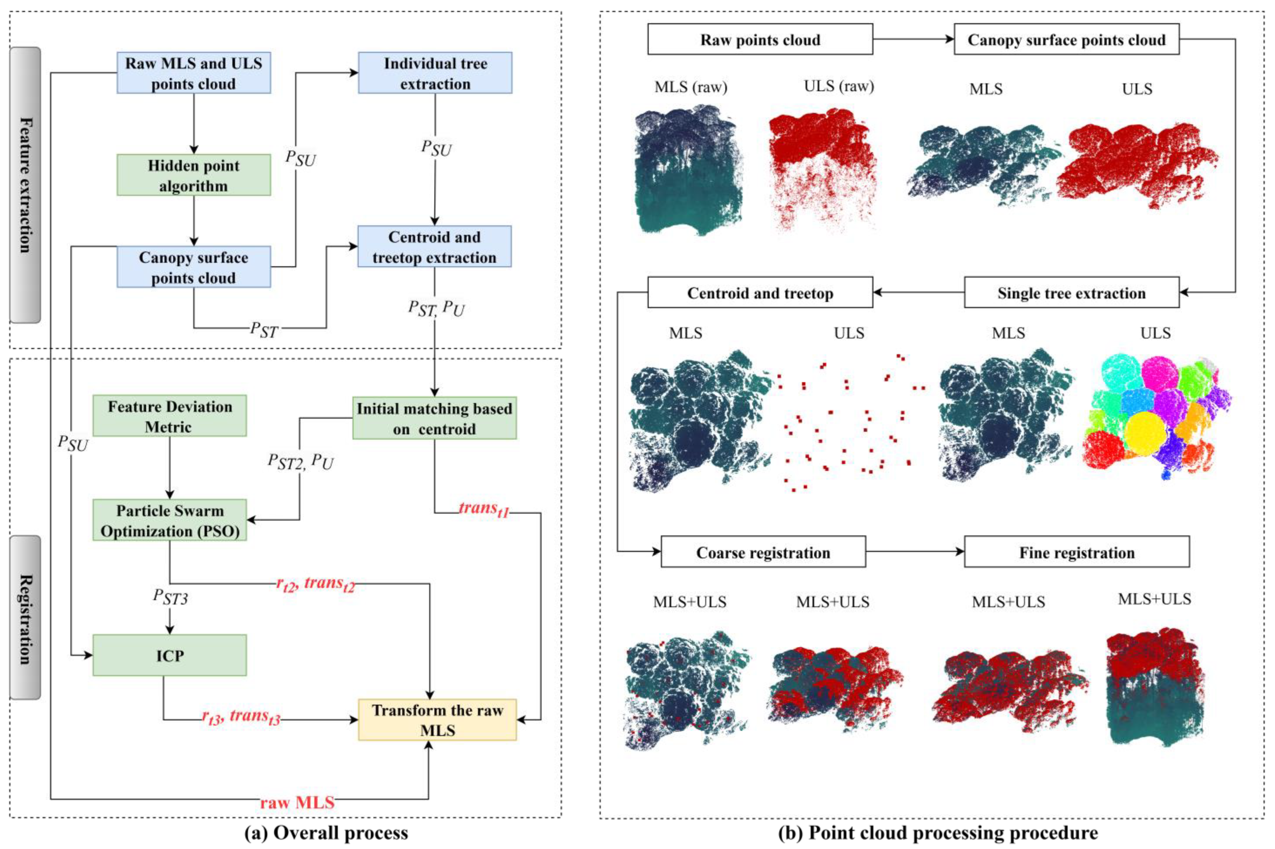
The datasets described above were utilized to validate the proposed method’s ability to achieve accurate registration in high-canopy-density forests. In this paper, we propose a point cloud registration methodology for ULS and MLS forest point clouds, which involves two primary processes: feature extraction and registration, as illustrated in Figure 2.

During the feature extraction process, canopy surface point clouds based on MLS and ULS data are generated, respectively. Subsequently, individual trees were segmented from the ULS-derived surface point clouds, and the centroid coordinates and treetop coordinates of each tree were computed. In the coarse registration process, a Feature Deviation Metric (FDM) is introduced to establish geometric correspondences between individual tree features extracted from ULS data and surface point clouds of MLS data. Taking the FDM as the objective function, a Particle Swarm Optimization (PSO) algorithm is employed to iteratively search for optimal rotation and translation parameters for coarse alignment. In the fine registration phase, an Iterative Closest Point (ICP) algorithm is applied to achieve precise refinement of the registration by iteratively refining the transformation parameters derived from coarse registration, thereby realizing precise spatial registration of the two point cloud datasets. The core part of this method is to use the FDM algorithm to register the point cloud of the canopy surface; thus, this registration method can be abbreviated as surface-FDM.

3.1. Feature Extraction

3.1.1. Extraction of Canopy Surface Point Cloud

The point clouds obtained from ULS and MLS exhibit overlapping features on the canopy surface. Leveraging this overlap, extracting surface features from both datasets can effectively enhance registration efficiency by mitigating interference from extraneous data [9]. In this study, a radius-based filtering algorithm [24] was first applied to denoise the point clouds. This algorithm involves the following steps: (1) For each point, identify neighboring points within a specified radius (Points with a distance of less than 2 m will be considered as neighbor points). (2) Determine whether to retain or filter points based on the number of neighbors or other criteria. Here, points with fewer than 5 neighbors are deleted.

Subsequently, the hidden point algorithm (HP) is used to extract the canopy surface point clouds. Hidden points refer to those points that become occluded and are not visible from a given viewpoint after surface reconstruction of the point cloud [25].

This algorithm was proposed by Katz et al. The algorithm consists of two parts: point cloud transformation and convex hull construction.

Point Cloud Transformation: Given a point set P and C, associate P with a coordinate system and place C at the origin. A function is then required to map each point p_i (where p_i ∈ P) onto the ray from C to p_i, such that it monotonically decreases along ‖p_i‖, where ‖⋅‖ denotes a norm. In Katz’s paper, the method of spherical flipping inversion was used, which links the D-dimensional sphere with radius R centered at C to a sphere that contains all points of P.

The Equation for the mirrored reflection of $p_i$ is:

$$\widehat{p_i}=f\left(p_i\right)=p_i+2\left(R-{\Vert p}_i\parallel \right){\displaystyle \frac{p_i}{{\Vert p}_i\Vert }}$$

(1)

Convex Hull Construction: A convex hull is constructed for the union of the transformed point cloud $\widehat{P}$ and the origin C, $\widehat{P}\cup \left\{C\right\}$. The points on the convex hull correspond to the visible points in the original point cloud P.

Extracted ULS and MLS canopy surfaces are denoted as P_SU and P_ST, respectively.

3.1.2. Extraction of Individual Tree Feature

The individual tree extraction from ULS canopy surface point clouds involves two primary stages: firstly, applying the voxel down-sampling method to reduce point cloud density and enhance computational efficiency [26,27], and subsequently, computing treetop coordinates and the centroid of each individual tree.

Traditional methods for treetop determination rely on local maxima, which limit their applicability in broadleaf forests [28]. Additionally, using point-to-treetop distance alone to determine tree membership has significant limitations. To address these challenges, we developed an individual tree extraction method based on a dual-threshold approach—named DIT (Double-threshold for point-to-centroid and point-to-tree distances, Individual, Tree extraction)—to derive tree centroids and treetops, as detailed in Appendix A Algorithm A1.

Our new method utilizes both the distance from points to the tree centroid (3D (x, y)) and the distance from points to the nearest tree (3D (x, y, z)) to make a comprehensive determination of whether a point belongs to an existing tree. The equation is as follows:

$$d_c=distance\left(2D\left(x,y\right)\right)=\sqrt{{\left(x_a-x_b\right)}^2+{\left(y_a-y_b\right)}^2}$$

(2)

$$d_t=distance\left(3D\left(x,y,z\right)\right)=\sqrt{{\left(x_a-x_c\right)}^2+{\left(y_a-y_c\right)}^2+{\left(z_a-z_c\right)}^2}$$

(3)

Here, a denotes the point to be segmented, b denotes the centroid of the tree, and c denotes a point in the tree point cloud.

The centroid of the tree continuously changes as new points are added, providing greater flexibility. The equation is as follows:

$$d={\displaystyle \frac{d_c}{{\beta }_1}}+{\displaystyle \frac{d_t}{{\beta }_2}}$$

(4)

d is a criterion, which can be found on line 15 of Appendix A (Algorithm A1). β₁ and β₂ are two fixed parameters. β₁ is the maximum radius of trees in that area. β₂ is an empirical parameter used to limit the size of d_t and needs to be defined by the user. For recommendations on the choice of β₂, please refer to the Discussion section.

The centroid of each individual tree is calculated by averaging the coordinates of all points in its point cloud, as shown in the following equations:

$$center\left(P\right)=\left({\displaystyle \frac{1}{o}}\sum _o^o{x}_l,{\displaystyle \frac{1}{o}}\sum _o^o{y}_l,{\displaystyle \frac{1}{o}}\sum _o^o{z}_l\right)$$

(5)

where P is a point cloud, o represents the total number of points in the point cloud.

3.2. Registration

The registration process developed in this paper primarily consists of the following steps: (1) A constrained search space was established using the geometric boundaries extracted from MLS and ULS point clouds. (2) A novel Feature Deviation Metric (FDM) was proposed to quantify inter-feature relationships between individual tree features extracted from ULS data and surface point clouds of MLS data, serving as the evaluation criterion for alignment candidates. (3) Particle Swarm Optimization (PSO) was employed to iteratively search for the optimal transformation parameters within the predefined search space. (4) To refine the alignment accuracy, the ICP (Iterative Closest Point) algorithm [29] was applied for fine-grained registration.

3.2.1. Construction of Search Space

The search space construction aims to constrain the parameter optimization domain for point cloud registration.

First, the individual tree feature points from ULS and the canopy surface points from MLS are coarsely aligned using their centroids as initial references. The transformation equation is:

$$tran{s}_{t1}\left(x,y,z\right)=center\left(P_U\right)-center\left(P_{ST}\right)$$

(6)

$$P_{ST2}=P_{ST}+tran{s}_{t1}\left(x,y,z\right)$$

(7)

where P_ST2 is the points cloud after centroid translation, P_U is the ULS point cloud (reference point cloud) after individual tree feature extraction. P_ST is the MLS canopy surface point cloud (target point cloud). trans_t1(x, y, z) is the translation amount of the target point cloud in the (x, y, z) directions for registration. Center (*) is the function to extract the centroid of the point cloud.

Subsequently, alignment is performed under the assumption that both ULS and MLS systems maintain consistent z-axis orientation during data acquisition. This constraint allows rotational and transformation adjustments to be confined exclusively to the (x, y) plane. Using Euler angles [30], we can obtain the rotation matrix as shown in Equation (8).

$$r=\left[\begin{array}{ccc}cos\theta & -sin\theta & 0\\ sin\theta & cos\theta & 0\\ 0& 0& 1\end{array}\right]$$

(8)

where r is the rotation matrix, θ is the rotation angle, and θ $\in$ (0, 2π); then, the set of all possible r is shown in Equation (9):

$$R=\left\{r|\theta \in (0,2\pi )\right\}$$

(9)

Equation (10) represents the set of translation parameters for constructing the search space.

$$Trans=\left\{\begin{array}{c}trans\left(x,y\right)|\\ x\in \left(-X_{thord},X_{thord}\right),y\in -Y_{thord},Y_{thord}\end{array}\right\}$$

(10)

where trans(x, y) is a set of point pairs containing (x, y) coordinates, and X_thord and Y_thord are the translation ranges in the x and y directions, respectively. The values of X_thord and Y_thord are determined by the size of the plot.

Equation (11) represents the set of translation and rotation parameters for constructing the search space.

$$Method=\left(R,Trans\right)$$

(11)

Suppose a certain scheme is denoted as Method_i, rotation and translation parameters r_i, trans_i This results in the transformed point cloud is shown in Equation (12)

$$P_i=P_{ST2}{r}_i+tran{s}_i\left(x,y\right)$$

(12)

3.2.2. Construction of Feature Deviation Metric

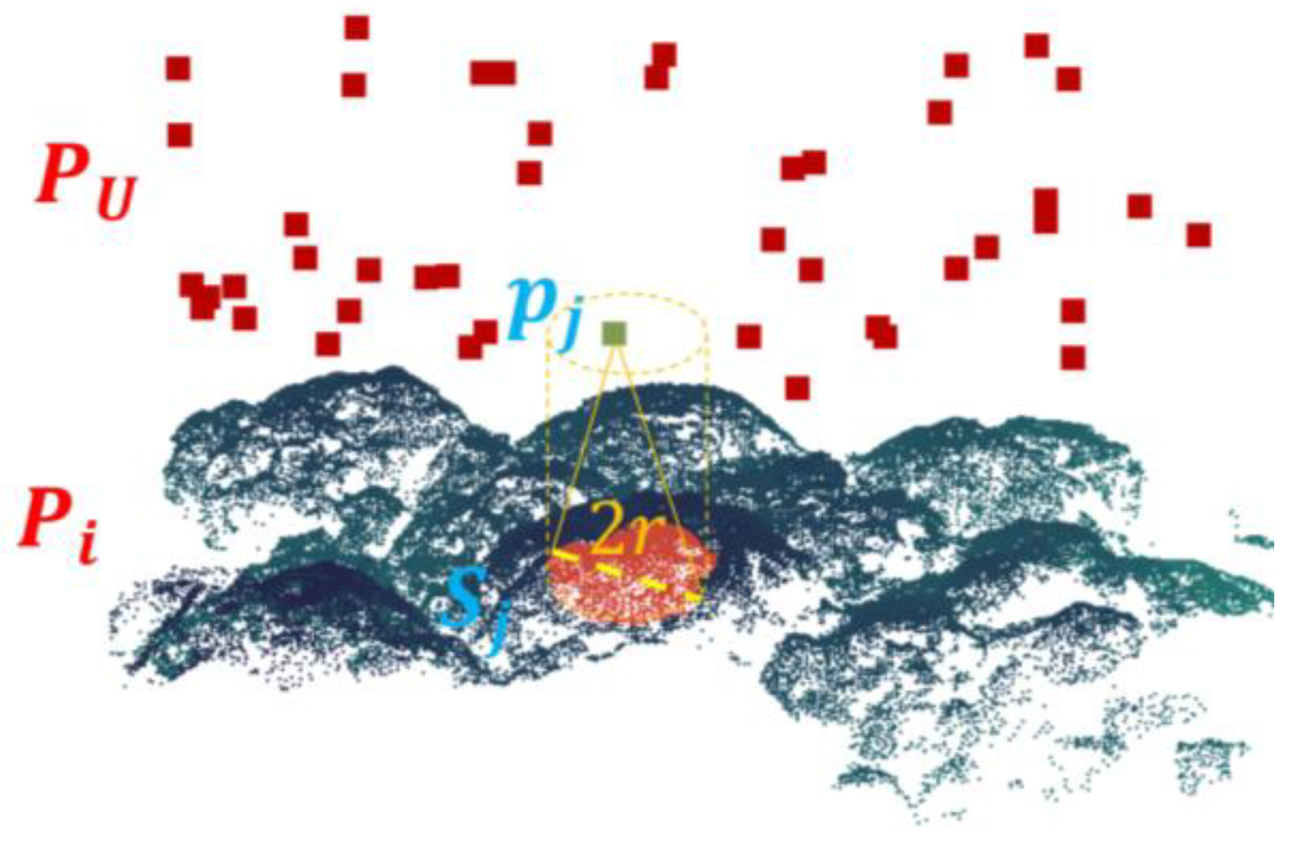
The Feature Deviation Metric (FDM) is proposed to quantify correspondences between individual tree features extracted from ULS data and canopy surface points from MLS. Serving as the objective function for the subsequent coarse registration algorithm, FDM computation employs a cylindrical search strategy, as illustrated in Figure 3.

For a point p_j ∈ P_U, define a cylindrical search region with its central axis passing through p_j and aligned with the z-axis, and a radius r = 5 × voxel size. Extract all points in P_U within this cylinder to form the set S_j, then compute the average z-axis deviation between p_j and points in S_j.

$$d_i={\displaystyle \frac{1}{m}}\sum _{k=1}^m\left(z_j-z_{jk}\right)$$

(13)

where m is the number of the point in S_j, z_j is the z-coordinate of point p_j, z_jk is the z-coordinate of a point in set S_j. Using this method, a cylinder is constructed for each point in P_U, and the corresponding mapping is obtained in P_i, thus forming a Deviation Metric.

The variance $v_i$ of these n points—serving as the objective function, is expressed as:

$$v_i={\displaystyle \frac{1}{n}}\sum _{j=1}^n{\left(d_j-\overline{d}\right)}^2$$

(14)

Here, n is the number of ULS point clouds after extracting individual tree features (P_U), and $\overline{d}$ is the average of these differences.

3.2.3. Coarse Registration

During coarse registration, the validity of rotation and translation parameters is evaluated by calculating the variance of the Feature Deviation Metric (FDM). In this paper, a Particle Swarm Optimization (PSO) algorithm [31] is employed to locate the optimal transformation parameters (rotation and translation) that minimize the FDM variance. When $v_i$ reaches its minimum, the corresponding scheme Method_i is identified as the optimal solution, with the rotation matrix denoted as r_t2, with the translation denoted as $tran{s}_{t2}\left(x,y,0\right)$. The coarse registration result is expressed as:

$$P_{ST3}=\left(P_{ST2}\right)r_{t2}+tran{s}_{t2}\left(x,y,z\right)$$

(15)

where P_ST3 is the MLS canopy surface point cloud after coarse registration. In $tran{s}_{t2}\left(x,y,z\right)$, Since z-axis translation was not considered during the search, the z-axis translation amount is computed as the average of z-coordinate differences at the optimal solution, denoted as $\overline{d}$.

3.2.4. Fine Registration

For the coarsely registered MLS canopy surface point cloud (P_ST3), the Iterative Closest Point (ICP) algorithm is employed for registration to derive precise rotation and translation parameters. Based on the ICP algorithm, the MLS canopy surface point cloud after coarse transformation (P_ST3) and the ULS canopy surface point cloud (PSU) are registered. The resulting rotation matrix and translation parameters are denoted as r_t3 and trans_t3(x, y, z), respectively.

3.2.5. Transform the Raw MLS

Applying final transformation to the raw complete MLS point cloud by using Equation (16):

$$ML{S}_{reg}=\left[\left(ML{S}_{raw}+tran{s}_{t1}\right)r_{t2}+tran{s}_{t2}\right]r_{t3}+tran{s}_{t3}$$

(16)

where MLS_raw represents the raw MLS point cloud without any processing, while MLS_reg represents the MLS point cloud after final registration.

3.3. Accuracy Verification

To quantify the performance of the proposed method, this paper employs manual methods to identify tree canopy apexes and trunk intersection points in ULS and MLS data as reference points. The method’s accuracy is evaluated by computing the distances between registered reference points from ULS and MLS datasets, as well as the root-mean-square error (RMSE).

Additionally, to ensure the spatial uniformity of reference points within each plot, the point cloud was partitioned into a 3 × 3 grid in the plot’s horizontal (x, y) plane. By adopting a random selection approach, 1 to 2 validation points were designated per grid, ensuring that each plot contained 15 reference points.

Due to the varying degrees of sparsity of ULS and MLS data in different locations, when searching for corresponding points, the position of the final point is determined by averaging the points within a certain range (<0.1 m) around that point. The distance calculation is as follows:

$$distance=\sqrt{{{(x}_a-x_b)}^2+{{(y}_a-y_b)}^2+{{(z}_a-z_b)}^2}$$

(17)

Here, a is the reference point on the reference point cloud (ULS), and b is the corresponding point on the MLS point cloud after registration transformation.

The RMSE calculation equation is as follows:

$$RMSE=\sqrt{{\displaystyle \frac{{\sum }_{i=1}^{number}distanc{e}_i}{n}}}$$

(18)

where number represents the number of reference points, and distance is the Euclidean distance between a pair of reference points on the ULS and MLS point clouds.

3.4. Basis for Parameter Setting

To validate the generalization capability of the model, all experiments on the sample areas in our study were conducted under uniform parameters. The parameters obtained in our experiments are shown in

Table 2. Parameter settings in the model.

Method Section	HP		PSO					FDM
Parameter name	Camera	Radius	Swarm Size	Max Iter	Omega (ω)	Phip (c1)	Phig (c2)	${\beta }_1$	${\beta }_2$	Radius r	Voxel Size
Parameter value	x = Center(x) y = Center(y) z = Max(z) + (Max(z) − Min(z)) ∗ 3	z ∗ 100	1000	20	0.3	1.6	1.8	8	4	2	0.4

Note: Center(x) and Center(y) are the center points of sample areas x and y, respectively. Max(z) and Min(z) are the maximum and minimum values of z in the sample area, respectively.

. In our model, the HP algorithm, PSO algorithm, and FDM contain empirical parameters that need to be specified. Among these, the parameters for HP and PSO were set according to the recommendations of the original authors of these models. As for FDM, which is our own proposed model, we provided recommended values based on experiments across different sample areas.

3.5. Comparative Experiment Design

This paper presents a point cloud registration method for ULS and MLS in high canopy closure forest areas, which is based on feature extraction and feature relationship construction. In the feature extraction part, we propose a DIT individual tree segmentation method. For feature relationship construction, we introduce an FDM approach to establish feature correspondences. To assess the efficacy of DIT and FDM, we devised comparative schemes (as detailed in Table 4), evaluating: ① the quantity of plots successfully registered by each model (with RMSE < 1.5); ② the overall fine registration accuracy of models within these valid plots.

4. Results

Based on the proposed method and experimental design, we conducted experiments across 14 plots in two different regions. This section aims to illustrate the performance results of the proposed method for registering ULS and MLS point clouds in high-canopy-density forest areas.

4.1. Overview of Results

Figure 4 is the visual display of the registration results for 2 plots. For each plot, the first image shows the top view of the plot, the second shows the overall registration effect, and the third provides a side view of a specific small region. Visually, after registration, the canopy apexes and contours of the ULS and MLS point clouds in 2 plots align well, the positions of the trunks are accurately registered, and the ground point clouds exhibit effective overlap (detailed results are shown in Appendix B). As can be seen from the result graph, although there are significant differences in vertical density between ULS and MLS, as well as substantial variations in horizontal coverage, our model is still capable of achieving registration.

Table 3. Summary of registration accuracy and effectiveness of 14 plots. Time (s) denotes the duration (in seconds, s) from importing original data to calculating the transformation matrix. RMSE represents the root mean square error. Z-axis deviation (°) is the z-axis deviation across the plots.

Plot	Time (s)	RMSE of Coarse Registration	RMSE of Fine Registration	Z-Axis Deviation (°)
1	30	0.788	0.096	1.65
2	28	0.337	0.110	1.28
3	29	1.161	0.110	1.93
4	33	0.659	0.118	1.62
5	32	0.931	0.124	1.28
6	28	1.143	0.127	1.90
7	36	0.867	0.166	1.16
8	30	1.749	0.514	2.17
9	36	0.427	0.086	2.13
10	40	0.348	0.036	0.34
11	30	1.901	0.027	0.84
12	31	0.590	0.077	0.50
13	32	0.620	0.036	1.10
14	35	0.586	0.045	0.36

summarizes the registration accuracy and effectiveness of 14 plots. In this table, Time denotes the duration (in seconds, s) from importing original data to calculating the transformation matrix. RMSE represents the root mean square error. As shown in the table, the model has an average RMSE of 0.119. The 14 plots in this experiment feature diverse slopes (ranging from 1° to 23°) and canopy densities (0.65 to 0.97), indicating that the model achieves high precision under different slope and canopy density conditions. This demonstrates its strong adaptability to varying environmental parameters. The registration experiments were conducted on a laptop equipped with an Intel i7-12700H CPU and 12 GB RAM, processed entirely via CPU, with an average processing time of 32 s. This suggests that the model balances time efficiency with low RMSE performance, maintaining computational effectiveness while ensuring registration accuracy.

4.2. Comparison of Different Algorithms

To demonstrate the advantages of our model, we conducted comparisons with several existing methods, including RANSAC [32], FGR [33], Deep Closest Point(DCP) [34], Point Cloud Registration Network (PCRNET) [35], and GeoTransformer [36].

First, to assess the effectiveness of different feature extraction methods in coarse registration for ULS and MLS in high canopy closure forests, we compared DIT (the method proposed in this study) with the commonly used forestry method LM in the registration model (schemes 1, 2, 3, and 4). When coarse registration utilized the FDM for constructing feature correspondences and PSO for feature search, the registration model integrated with the DIT algorithm successfully registered 14 plots—significantly outperforming the LM-integrated model, which only registered 11 plots. In the overlapping plots where both algorithms succeeded, the RMSE of the LM-based model was 0.231 units higher than that of the DIT model, indicating lower registration accuracy. When RANSAC was employed for coarse registration, the DIT-integrated model registered 5 plots, compared to 3 by the LM model. Overall, the DIT-integrated model outperforms the LM-based model in both accuracy and adaptability, owing to its iterative tree detection and adaptive centroid calculation. Unlike LM’s reliance on local maxima, DIT reduces uncertainty in complex forests by dynamically identifying trees during growth, enhancing robustness in heterogeneous environments.

Secondly, to evaluate the impact of different relationship construction methods in the coarse registration of ULS and MLS in high canopy closure forests, we compared the FDM-based method proposed in this study with commonly used approaches such as RANSAC and FGR within the registration framework (schemes 5 and 6). Both RANSAC and FGR only successfully registered a subset of plots. Specifically, FPFH features [37] enabled alignment in 5 plots—outperforming FGR in the number of registrable areas. However, this combination still lagged behind our proposed method. Compared with other relationship-building methods, the advantages of FDM lie not only in further suppressing noise through multi-point matching within the cylindrical region but also in its use of variance to facilitate a robust global assessment of spatial relationships.

In addition to classical models, we employed deep learning approaches including DCP, PCRNET and GeoTransformer to register ULS and MLS point clouds across 8 plots (schemes 7, 8, and 9). Due to the limited research on deep learning-based forest point cloud registration and the lack of training data, the model we employ is a pre-trained model provided by the authors. While deep learning methods achieved high precision (average RMSE < 0.5) in successfully registered plots, they were limited to only a few plots. In high-canopy-density forests, structural complexity, lack of training data, and significant discrepancies between ULS and MLS point clouds hinder feature extraction and model generalization [38]. Thus, despite their accuracy, deep learning approaches show limited applicability for ULS-MLS registration in dense forest environments.

5. Discussion

The Results section demonstrates the capability of our model in achieving registration in high-canopy-density forests. In this section, we further discuss the model’s computational efficiency, parameter adaptability, and limitations.

5.1. The Effect of Downsampling on Computational Efficiency

Down-sampling exerts a significant impact on both the registration accuracy and computational efficiency of the model. An optimal down-sampling ratio can enhance computational speed while preserving registration precision. Thus, we investigated the correlation between down-sampling degree and registration accuracy. Using canopy density and registration accuracy as criteria, we selected three typical plots (1, 4, 8) to analyse the relationship among down-sampling level, RMSE, and transformation matrix computation time. As shown in Figure 5, smaller voxel sizes increase computation time and reduce RMSE. Beyond a voxel size of 0.4, computation time stabilizes with <3 s variation across plots. For RMSE, plots 1 and 8 show minimal deviation (≤0.03) across voxel sizes 0.1–1, while plot 4 exhibits a sharp RMSE surge to 7.59 after 0.4. These results indicate that within a certain range, the model is not sensitive to changes in down-sampling level and can find the optimal match between voxel size, RMSE, and time.

5.2. Impact of Individual Tree Parameters

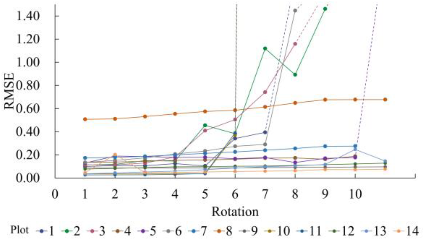
When performing individual tree extraction, the parameter d in Equation (4) serves as a key criterion for identifying individual tree points, and β₂ is a significant parameter within d. Since β₂ is an empirical parameter, it is necessary to investigate its impact on the model. The relationship between different values of β₂ and RMSE is shown in Figure 6. Within the parameter range of 0 to 6, the average RMSE across all 14 plots remained below 0.2, exhibiting minimal impact. The influence of β₂ showed variability among plots: Parameter β₂ has a slight effect on plots 5, 6, 7 and 10, but exhibits negligible sensitivity in the other 10 plots.

The results indicate that within a certain range, variations in parameter β₂ have little impact on the RMSE of the registration in most plots, demonstrating that the model is not sensitive to β₂ and has good applicability. However, since β₂ is an empirical parameter, users need to adjust it according to actual conditions.

5.3. Impact of z-Axis Deviation

When constructing the FDM, the model assumes that the z-axis direction of the MLS system is consistent with that of the ULS during measurement (both pointing in the direction of increasing elevation). However, the z-axis orientation of the MLS point cloud is likely to deviate due to errors caused by system errors and different operators during measurement, which can impact the registration.

To explore the impact of z-axis deviation on the model, artificial rotation was applied to the original MLS data. The entire point cloud was rotated around the centroid, altering the orientation of the z-axis. Using the model presented in this paper, the registration of rotated point clouds yields the results shown in Figure 7. When the deviation is within 5°, the average RMSE increases by 0.07, with almost no impact on the accuracy across the 14 sample areas, allowing the model to maintain high precision. Calculations of the z-axis angular deviations from field-measured data revealed that deviations between MLS and ULS across all 14 plots were below 3° (as shown in Table 4), demonstrating that angular deviations along the z-axis under standard operational conditions do not significantly impact the accuracy of current models.

Table 4. Comparison of different registration algorithms (RMSE). The meaning of ‘NAN’ indicates that registration is not possible (RMSE < 1.5). When the RMSE exceeds 1.5, it is considered unregistrable.

Scheme	Plot	The Number of Registrable Plots	Average RMSE at Registrable Plots
1	FDM-based registration (DIT) + ICP	14	0.120
2	FDM-based registration (LM) + ICP	11	0.351
3	LM + RANSAC + ICP	3	0.191
4	DIT + RANSAC + ICP	5	0.224
5	FPFH + ICP	5	0.460
6	FGR + ICP	4	0.449
7	DCP + ICP	2	0.175
8	PCRNET + ICP	3	0.470
9	GeoTransformer + ICP	4	0.180

Table 4. Comparison of different registration algorithms (RMSE). The meaning of ‘NAN’ indicates that registration is not possible (RMSE < 1.5). When the RMSE exceeds 1.5, it is considered unregistrable.

Scheme	Plot	The Number of Registrable Plots	Average RMSE at Registrable Plots
1	FDM-based registration (DIT) + ICP	14	0.120
2	FDM-based registration (LM) + ICP	11	0.351
3	LM + RANSAC + ICP	3	0.191
4	DIT + RANSAC + ICP	5	0.224
5	FPFH + ICP	5	0.460
6	FGR + ICP	4	0.449
7	DCP + ICP	2	0.175
8	PCRNET + ICP	3	0.470
9	GeoTransformer + ICP	4	0.180

5.4. Limitation

This paper utilizes the HP algorithm to extract MLS canopy surface point clouds for registration. However, excessive canopy overlap can result in substantial loss of canopy surface information, potentially undermining registration performance.

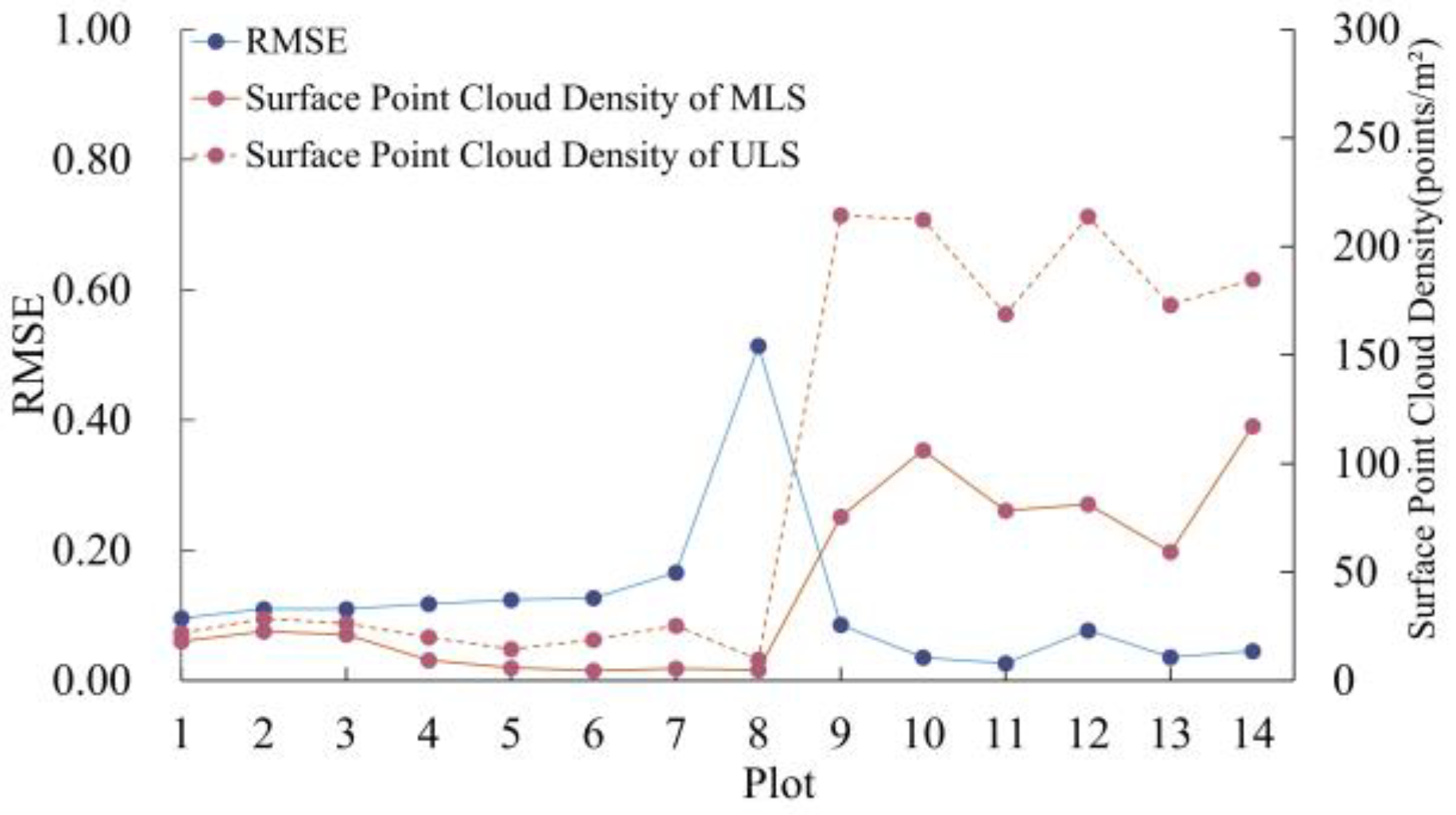
Figure 8 shows the relationship between canopy surface point cloud density and RMSE extracted using the Hidden Points algorithm in various plots. Due to measurements being taken from different platforms, both ULS and MLS surface point clouds were voxel down-sampled to a scale of 0.1 m for comparison. The figure indicates that lower densities of the crown surface point cloud correlate with higher RMSE values. In addition, we conducted a correlation analysis between surface point cloud density and RMSE, with the results shown in

Table 5. Correlation analysis between surface point cloud density and RMSE. The correlation coefficients are Spearman [39] and Kendall [40].

	Spearman		Kendall
	Spearman	p	Kendall	p
Surface Point Cloud Density of MLS	−0.90	0.00	−0.75	0.00
Surface Point Cloud Density of ULS	−0.79	0.00	−0.55	0.00

. For the relationship between MLS surface point clouds and RMSE, Spearman and Kendall correlations were −0.90 and −0.75, respectively, with a p-value less than 0.05, indicating a strong negative correlation between RMSE and MLS canopy surface point cloud density at a 95% confidence interval.

Additionally, from plot 4 to plot 8, RMSE increases from 0.12 to 0.51. Furthermore, in all 14 plots, MLS surface point cloud density is lower than ULS surface point cloud density. Notably, the RMSE in plot 8 is 0.51, which is significantly higher than the average RMSE of 0.089 for the other seven sample areas. Figure 9 depicts the registration results of plot 8, where the elevation of the MLS point cloud after registration is higher than it should be. This indicates that due to the sparse canopy surface point cloud of MLS, the canopy surface point cloud extracted using the HP algorithm includes fewer points from the upper layers of the canopy surface compared to ULS. Consequently, this results in elevation misalignment during registration.

To further explain the reason for the sparse surface point cloud, we extracted MLS point cloud density, canopy density (represented by the point cloud density above 0.5 times the stand height), and other related information from plots of the same type as plot 8 (plots located in the Malaysian region) for further analysis (

Table 6. The point cloud density and canopy conditions (represented by the point cloud density above 0.5 times the stand height) of MLS for sample plots similar to plot 8.

Plot	1	2	3	4	5	6	7	8
Point cloud density of MLS (pt/m2)	4765	6328	4707	3970	3276	5901	7678	4548
Point cloud density above 0.5 Tree Height of MLS (pt/m2)	249	182	165	273	184	282	295	478

). The results showed that the point cloud density above 0.5 times the stand height in plot 8 was 478 pt/m², which is much higher than the average value (263 pt/m²). However, as shown in Figure 8, the surface point cloud density of plot 8 from MLS was lower than that of the other plots. This indicates that the canopy density in plot 8 is higher than in other plots, which obstructed the laser penetration to the crown surface. Therefore, we conclude that canopy overlap and occlusion led to sparse MLS point clouds at the upper canopy layer, which in turn caused the MLS-derived elevations during registration to be higher than the actual elevations.

6. Conclusions

The registration of ULS and MLS point clouds in forested areas has always been a challenging task. This paper proposes an efficient and reliable registration model for ULS and MLS point clouds in high-canopy-density broadleaf forest regions. Through the individual tree feature clustering-based Feature Deviation Metric, we effectively extracted the features of forest ULS and MLS point clouds and established the correspondence between the point cloud to be registered and the reference point cloud.

In high-density plots in Malaysia and China, although the tree crowns in the plot are dense, the forest is highly stratified with almost no forest gaps, and the ULS point cloud has almost no points beneath the canopy, the model still demonstrated high accuracy and efficiency. Additionally, even when accounting for the vastly differing forest conditions between Malaysia and Northern China, the model still achieves impressive accuracy, further demonstrating its strong adaptability. Compared to other algorithms, the proposed registration model shows greater adaptability, better accuracy, and improved stability. Furthermore, through the analysis of the model’s internal parameters and external factors, it was found that the model shows good adaptability to internal parameters. Within a certain parameter range, it can maintain high accuracy, indicating that the model can effectively operate under varying environmental conditions, thus demonstrating significant practical value.