Automatic Rooftop Solar Panel Recognition from UAV LiDAR Data Using Deep Learning and Geometric Feature Analysis

Highlights

What are the main findings?

• Developed a Machine Learning approach using drone-based LiDAR point clouds to classify rooftop solar panels from building surfaces.
• Achieved very high classification accuracy, with F1 scores of 99% for commercial-scale panels and 95–96% for residential-scale panels.

What is the implication of the main finding?

• LiDAR geometry and reflectance features enable reliable rooftop solar detection, overcoming limitations of imagery-based methods that are often obstructed by trees, shadows, and roof orientation.
• Provides a scalable approach for applying ML-based classification to unlabelled urban datasets, supporting solar energy mapping and planning.

Abstract

As drone-based Light Detection and Ranging (LiDAR) becomes more accessible, it presents new opportunities for automated, geometry-driven classification. This study investigates the use of LiDAR point cloud data and Machine Learning (ML) to classify rooftop solar panels from building surfaces. While rooftop solar detection has been explored using satellite and aerial imagery, LiDAR offers geometric and reflectance-based attributes for classification. Two datasets were used: the University of Southern Queensland (UniSQ) campus, with commercial-sized panels, both elevated and flat, and a suburban area in Newcastle, Australia, with residential-sized panels sitting flush with the roof surface. UniSQ was classified using RANSAC (Random Sample Consensus), while Newcastle’s dataset was processed based on reflectance values. Geometric features were selected based on histogram overlap and Kullback–Leibler (KL) divergence, and models were trained using a Multilayer Perceptron (MLP) classifier implemented in both PyTorch and Scikit-learn libraries. Classification achieved F1 scores of 99% for UniSQ and 95–96% for the Newcastle dataset. These findings support the potential for ML-based classification to be applied to unlabelled datasets for rooftop solar analysis. Future work could expand the model to detect additional rooftop features and estimate panel counts across urban areas.

1. Introduction

Light Detection and Ranging (LiDAR)-equipped airborne platforms, such as drones or manned aircraft, are now widely used in surveying, environmental modelling and urban planning. Despite the restrictions of using Unmanned Aerial Vehicles (UAV) in urban areas [1], UAV based LiDAR can capture points at high density, hundreds of points per square metre, while maintaining exceptional positional accuracy (5–10 cm) [2]. These accuracies depend on factors such as flight altitude, scan angle, GNSS-IMU calibration and platform stability, which may vary across UAV systems. Despite these limitations, these capabilities allow 3D mapping of urban environments, including building rooftops. However, processing these large datasets is a challenging task, due to their size, number of points, and the need for specialised software [3]. Manual classification is time-consuming, prone to subjectivity, and difficult to scale [4]. With the increased use of drones in various applications, there is a growing demand for automated classification of aerial-based LiDAR data. One critical area of interest is the detection of solar panels in urban areas. For meeting renewable energy goals, understanding the distribution of solar installations is essential.

Previous studies have explored the potential for solar panels, considering factors such as the roof surface area, solar incidence and panel efficiency [5,6], rather than directly detecting panels themselves. Jiang et al. [7] explored the use of Deep Learning (DL) for solar panel segmentation across varying spatial resolutions, using satellite, aerial and UAV imagery, at 0.8 m, 0.3 m, and 0.1 m, respectively. They found that the spatial resolution matters, with higher resolution imagery boosting segmentation. Clark and Pacifici [8] developed a high-resolution dataset consisting of solar panels derived from satellite imagery manually annotated using QGIS. Their dataset was used to support the training of object detection models such as YOLO (You Only Look Once), which can automatically detect and localise solar panels from overhead imagery, using bounding boxes and class labels. While their work showed strong detection performance in 2D imagery, it did not utilise elevation data or 3D geometric features that may enhance classification in urban areas. Duran et al. [9] classified both photogrammetric and LiDAR point clouds using nine ML algorithms. Their focus was on building, ground, and high and low vegetation. Their MLP model showed the best accuracy at 96%, with Random Forest (RF) being a close second at 91%. While their study utilised geometric features, such as eigenvalues, planarity and roughness, there was a lack of analysis for choosing the best features that may have leveraged more use from their dataset.

Conversely, Amakhchan et al. [10] and Tarsha Kurdi et al. [2] performed a histogram analysis of geometric features, highlighting that careful feature selection, informed by the distribution of these features, can enhance classification accuracy in LiDAR datasets. Perhaps the closest study related to this one is by Kushwaha et al. [11], who aimed to extract rooftop solar panels from a photogrammetric point cloud. Their method involved computing the normal vector of each point to classify roof, façade, and panel surfaces based on the Z-component. While their approach demonstrates separation of panels from roof structures, it relied on rule-based classification rather than machine learning. Furthermore, it did not incorporate geometric feature analysis or any model evaluation, such as accuracy or F1 score. Based on the literature review, there remains a clear gap in the classification of installed rooftop solar panels from LiDAR-derived point clouds. This study addresses that gap by focusing on the following objectives.

• Evaluate the effectiveness of geometric and spectral features for differentiating rooftop solar panels from rooftop surfaces using LiDAR data.
• Compare the performance of two MLP-based deep learning models, developed using PyTorch and Scikit-learn, for supervised classification of roof and solar panels.
• Assess classification performance across two urban datasets (UniSQ and Newcastle), with UniSQ having commercial structures and Newcastle being primarily residential, using evaluation measures such as F1-score and overall accuracy.

The following sections outline the methodology used to achieve these objectives. This includes the classification process and dataset preparation, the selection of geometric and spectral features, an overview of how the MLP models were developed and refined, and a discussion on how model performance was evaluated.

2. Materials and Methods

This section describes the datasets, feature extraction, and classification methods used in this study. It is structured as follows: Section 2.1 and Section 2.2 introduce the datasets and feature engineering, Section 2.3 outlines the input features including RGB, and Section 2.4 details the classification workflow.

2.1. Datasets

2.1.1. UniSQ Dataset

The first dataset was collected over a large commercial rooftop at the University of Southern Queensland using a RIEGL miniVUX-3UAV LiDAR sensor and a Sony Alpha series RGB camera mounted on a UAV. Flights were conducted at 80 m AGL, 8 m/s forward speed, with a 120° scan angle and a pulse repetition rate equivalent to 54 scan lines per second. Data were processed in RiPROCESS, which implemented extrabytes to store reflectance attributes.

The dataset contained 227,410 total points. Two buildings were analysed: A block with elevated panels (Figure 1) and D block with flat panels (Figure 2). RANSAC [12] plane segmentation effectively separated panels from roofs on A block, but D block required parameter adjustments due to minimal height differences. Outliers such as ducts and HVAC units were removed manually.

2.1.2. Newcastle Dataset

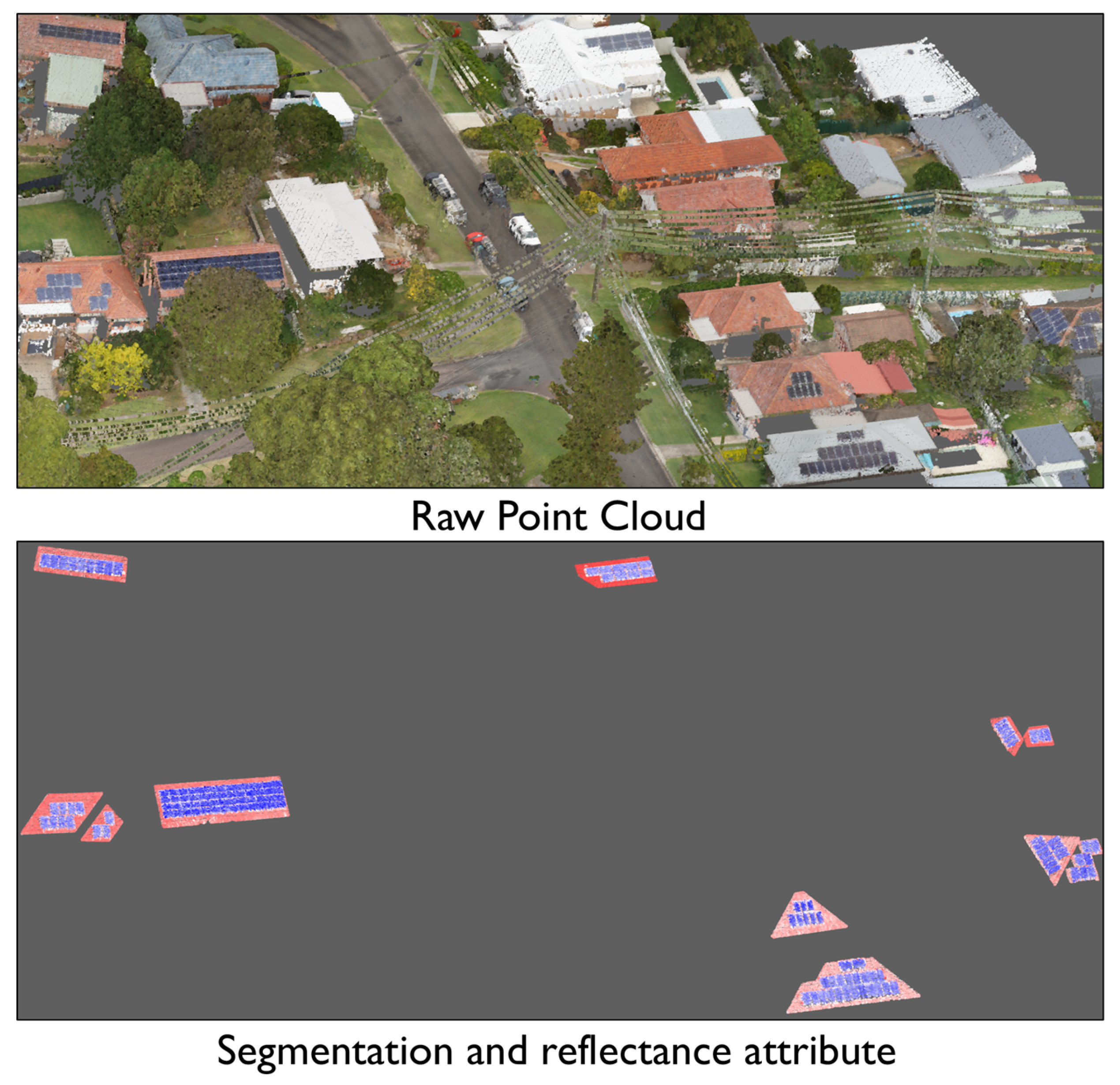
The second dataset was collected over a suburban residential area in Newcastle, Australia, using the same UAV-mounted RIEGL miniVUX-3UAV LiDAR sensor paired with a Sony Alpha series RGB camera. The dataset was processed with RiPROCESS, which implements extrabytes to store additional attributes such as reflectance. The RGB imagery was fused with the LiDAR point cloud, producing a colourised dataset with both geometric and spectral information. The raw point cloud was loaded into CloudCompare. Thirteen roof segments, including panels, were extracted from the dataset, for a total of 103,087 points (Figure 3). While RANSAC plane segmentation could be used to separate roof planes from panels, it required manual parameter tuning for each roof segment due to variations in slope, orientation, and roof structure. This limitation significantly increased preprocessing time and highlighted scalability issues for large-scale projects.

Instead, the reflectance attribute provided by the LiDAR was used as the primary discriminator. Reflectance is derived from amplitude but corrects for range dependency, making it more suitable for distinguishing surface materials across multiple scan positions. The amplitude formula is a ratio, given in the units of decibels (dB) [13].

$$A_{db}=10·\mathrm{l}\mathrm{o}\mathrm{g}({\displaystyle \frac{P_{echo}}{P_{DL}}})$$

(1)

where $A_{db}$ is the amplitude in decibels, $P_{echo}$ is the optical input power and $P_{DL}$ is the minimal detectable input power.

Because calibrated amplitude suffers from range dependence, it is not ideal for material classification. Reflectance instead expresses the fraction of incident optical power reflected by a surface at a given wavelength. Relative reflectance can be computed by comparing the amplitude of a target surface to that of a calibrated reference surface at the same range [13]. The formula for relative reflectance is:

$${\rho }_{rel}=A_{db}-A_{dB.ref}\mathrm{(R)}$$

(2)

where ${\rho }_{rel}$ is the relative reflectance in decibels, $A_{db}$ is the calibrated amplitude and $A_{dB.ref}$(R) is the amplitude of the reference target at range R.

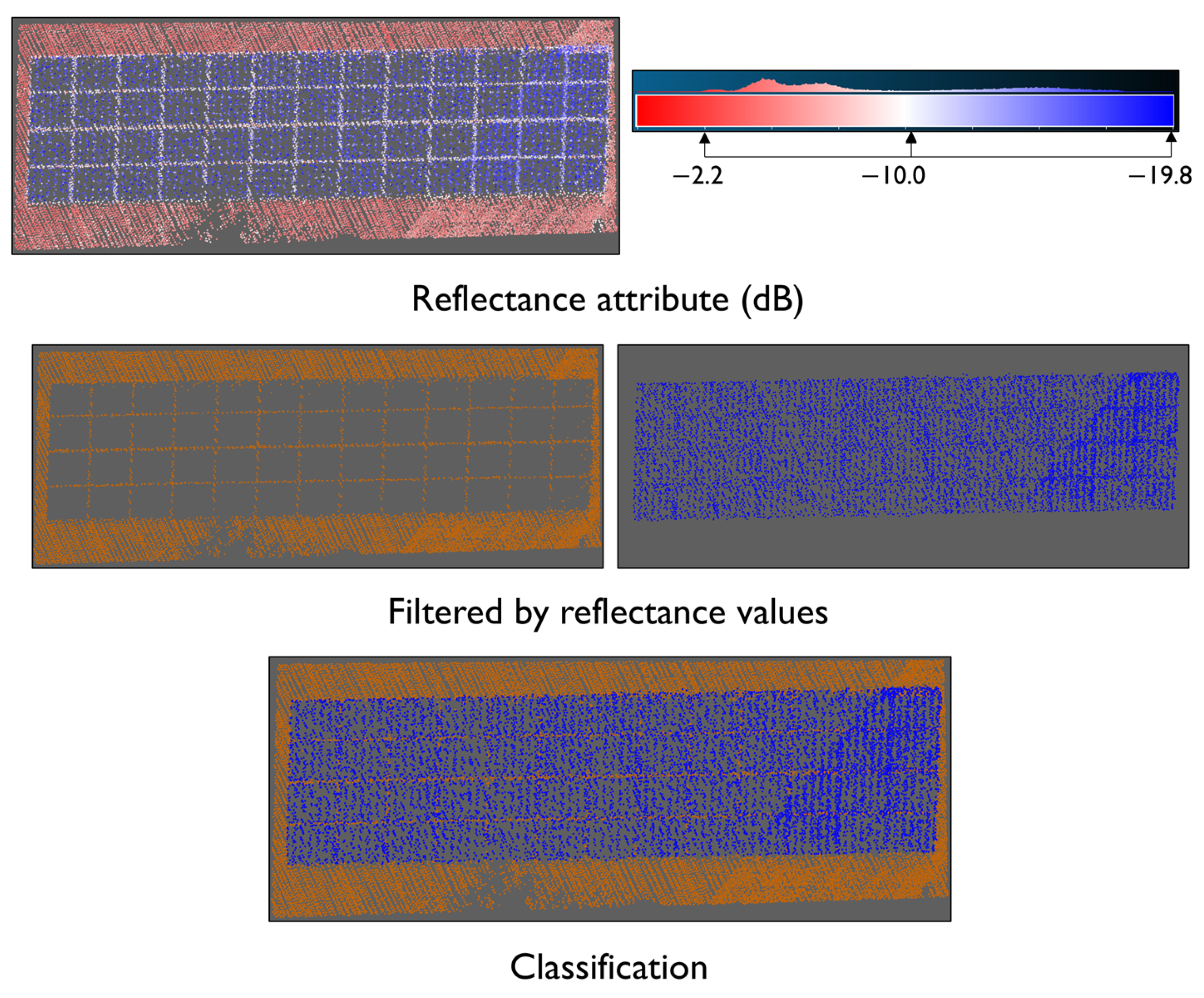
Reflectance values indicate how much of the laser pulse is returned to the sensor, providing a basis for material differentiation. More negative values correspond to surfaces that absorb more energy, while less negative values indicate stronger reflections. In the Newcastle dataset, solar panels consistently exhibited lower reflectance (−19.8 dB to −10 dB) than surrounding roofs (−10 dB to −2.2 dB) (Figure 4), reflecting their light-absorbing coatings.

Classification was performed in CloudCompare using the scalar field and filter-by-value tool, with colour mapping applied: blue for panels, red for roofs, and white for mid-range values. The latter corresponded to structural supports, which were included as roof to maintain a clear binary separation. Unlike in the UniSQ dataset, where such supports were discarded for A block, they were retained here due to their reflectance similarity with roof materials.

Because reflectance is expressed in decibels, even small numerical differences represent substantial changes in signal strength. Roofs, typically made of tile or metal, returned stronger signals, while solar panels absorbed more energy. Although RIEGL [13] notes that positive reflectance values are associated with retro-reflective surfaces such as traffic signs or windows, the solar panels in this dataset showed negative reflectance values due to their anti-reflective coatings.

2.2. Geometric Feature Selection

Geometric features are used to assess the relationship between each point in the point cloud and its surrounding neighbours [2]. Once spatial 3D information about the environment has been collected in the form of point clouds, the next step involves defining the local 3D neighbourhood of each point, $p=(x,y,z)$. This is achieved by applying a spherical neighbourhood, where all points within a sphere of fixed radius, $r$, around $p$ are considered part of its local neighbourhood $N$ [14].

The covariance-based features used in this study are derived from the eigenvalues, ${\lambda }_1>{\lambda }_2>{\lambda }_3\in \mathbb{R}$ and the corresponding eigenvectors $e_1,e_2,e_3,\in {\mathbb{R}}^3$ of the neighbourhood covariance matrix:

$$\mathrm{c}\mathrm{o}\mathrm{v}\left(N\right)={\displaystyle \frac{1}{\left|N\right|}} \sum _{p\in \mathrm{N} }(p-\overline{p}){\left(p-\overline{p}\right)}^T$$

(3)

Each point, $p$ represents a 3D location in the neighbourhood, $N$, which may be defined by a spherical radius. The covariance matrix describes how these points are distributed around their centroid point, $\overline{p}$ [15,16].

The geometric features calculated in this study using CloudCompare are derived from the methodology of Hackel et al. [15]. From the eigenvalues calculated in the spherical neighbourhood, several geometric features are derived. This follows the work of Tarsha Kurdi et al. [2], where multiple datasets were tested across various geometric features. These include, the sum of eigenvalues, omnivariance, eigenentropy, anisotropy, planarity, linearity, PCA1, PCA2, surface variation, sphericity, and verticality. The addition of roughness is included in our study to see if panels differentiate from roof surfaces.

The geometric features are defined below:

Sum of eigenvalues:

$$\sum {\lambda }_i={\lambda }_1+{\lambda }_2+{\lambda }_3$$

(4)

Omnivariance:

$$O= \sqrt[3]{{\lambda }_1·{\lambda }_2·{\lambda }_3}$$

(5)

Eigenentropy:

$$E= - \sum {\lambda }_1\ln \left({\lambda }_1\right)$$

(6)

Anisotropy:

$$A={\displaystyle \frac{{\lambda }_1-{\lambda }_3}{{\lambda }_1}}$$

(7)

Planarity:

$$P={\displaystyle \frac{{\lambda }_2-{\lambda }_3}{{\lambda }_1}}$$

(8)

Linearity:

$$L={\displaystyle \frac{{\lambda }_1-{\lambda }_2}{{\lambda }_1}}$$

(9)

PCA1:

$$PCA1={\displaystyle \frac{{\lambda }_1}{{\lambda }_1+{\lambda }_2+{\lambda }_3}}$$

(10)

PCA2:

$$PCA2={\displaystyle \frac{{\lambda }_2}{{\lambda }_1+{\lambda }_2+{\lambda }_3}}$$

(11)

Surface Variation:

$$S_v={\displaystyle \frac{{\lambda }_3}{{\lambda }_1+{\lambda }_2+{\lambda }_3}}$$

(12)

Sphericity:

$$S={\displaystyle \frac{{\lambda }_3}{{\lambda }_1}}$$

(13)

Verticality:

Verticality measures how much a surface deviates from being horizontal. It is derived from the surface normal vector $n \in {\mathbb{R}}^3$, where $n=\left(n_x,n_y,n_z\right)$ The verticality $V$ is calculated by:

$$V=1-\left|n_z\right|$$

(14)

Here, $n_z$ is the vertical component of the normal vector, which indicates how much a surface is aligned with the vertical axis [2,14,17].

The roughness calculation in CloudCompare is based on the distance between a point and the best-fitting plane computed from its neighbouring points [18]. The kernel size, defined as the spherical neighbourhood radius, was set to the default value for each dataset and applied across all geometric feature calculations. Preliminary testing with alternative values showed minimal impact on classification performance.

Histogram Overlap and KL Divergence

Having explored the shape and spread of each histogram, we can now assess how much the roof and solar panel classes overlap by using two statistical measures, histogram overlap and KL divergence.

Histogram overlap is calculated using the histogram intersection method proposed by Swain and Ballard [19]. This method computes the similarity between two normalised histograms by summing the minimum values of the corresponding bins.

$${\sum }_{j=1}^n\mathrm{m}\mathrm{i}\mathrm{n}(I_j,M_j)$$

(15)

where $I$ and $M$ are the histograms of the two distributions, in this case, the roof and the solar panels classes, and $n$ is the number of bins. This expression measures the overlapping area between distributions by taking the minimum value of each bin. A higher overlap value (approaching 1) suggests strong similarity between the classes, while a lower value (approaching 0) indicates greater class separability.

Amakhchan et al. [10] proposed a similar analysis known as Histogram Form Resemblance Mark (HFRM), which measured the overlap between histograms for vegetation and terrain classes. In their study, features with overlap values below 0.5 were selected for their DL classification model. In our study, because the geometric properties of roofs and solar panels are similar, we adopt a more flexible interpretation. Features that have an overlap value below 0.5 are considered strong, while those below 0.7 are still considered useful for class separation.

To further assess geometric feature separability, KL divergence was used to measure the difference between the probability density functions of the roof and panel classes. KL divergence measures how much information is lost when one probability distribution is used to approximate another [20]. This method has been applied in previous studies for feature selection, for classifying different dormer types on roofs [21].

The KL divergence, denoted as $D_{KL} \left(P\right|\left|Q\right)$, measures how a probability distribution $Q$, diverges from a reference distribution, $P$.

$$D_{KL}(P||Q)=\sum _{i}P\left(i\right)\log \left({\displaystyle \frac{P\left(i\right)}{Q\left(i\right)}}\right)$$

(16)

Here, $P$ and $Q$ represent the probability distributions of geometric feature values for either the roof or panel classes. This measures how different the two distributions are from each other. A higher KL divergence means greater separation between classes, while lower values suggest they are similar.

2.3. Selected Geometric Features

The selected features will be used to assess neighbourhood characteristics, including surface, shape, and distribution within the point cloud. These results will be implemented in the DL pipeline for identifying and distinguishing between roof and solar panel points. Seven features from each dataset were selected for their ability to clearly differentiate between the two classes.

Table 1. Selected geometric features highlighted in bold, for the UniSQ dataset based on histogram analysis and KL divergence.

Feature (UniSQ)	Histogram Overlap	KL Divergence (Roof||Panel)	KL Divergence (Panel||Roof)	Acceptance
Eigenvalues Sum	0.8	0.1	0.2	No
Omnivariance	0.2	2.4	2.1	Yes
Eigenentropy	0.8	0.1	0.2	No
Anisotropy	0.2	1.5	2.0	Yes
Planarity	0.6	0.6	0.4	Yes
Linearity	0.7	0.3	0.2	No
PCA1	0.8	0.1	0.1	No
PCA2	0.7	0.5	0.3	No
Surface Variation	0.1	3.5	2.4	Yes
Sphericity	0.2	1.5	2.0	Yes
Verticality	0.3	1.3	2.7	Yes
Roughness	0.6	0.5	0.8	Yes

and

Table 2. Selected geometric features for the Newcastle dataset are highlighted in bold, based on histogram analysis and KL divergence.

Feature (Newcastle)	Histogram Overlap	KL Divergence (Roof||Panel)	KL Divergence (Panel||Roof)	Acceptance
Eigenvalues Sum	0.5	1.4	0.7	Yes
Omnivariance	0.6	3.3	0.5	No
Eigenentropy	0.5	1.5	0.8	Yes
Anisotropy	0.7	0.4	0.2	No
Planarity	0.6	0.7	0.5	Yes
Linearity	0.6	0.8	0.5	Yes
PCA1	0.6	0.8	0.5	Yes
PCA2	0.6	0.8	0.5	Yes
Surface Variation	0.8	0.3	0.2	No
Sphericity	0.7	0.4	0.2	No
Verticality	0.8	0.4	0.1	No
Roughness	0.6	0.4	0.5	Yes

present the final selection based on the histogram overlap and KL divergence analysis discussed in the previous section.

2.3.1. UniSQ Feature Selection

The features that demonstrated the most effective separation between roof and solar panel classes, based on low histogram overlap (≤0.2) and high KL divergence (≥1), were omnivariance, anisotropy, surface variation, and sphericity. Surface variation recorded the highest KL divergence in both directions, showing the greatest difference between the two classes.

Verticality also showed strong separation, with an overlap value below 0.5 and KL divergence above 1 in both directions. Planarity, the weakest performer with an overlap value of 0.6, was retained for further analysis. Roughness, although not commonly highlighted in similar studies, scored comparably to planarity. This feature was kept, as it may capture subtle surface deviations that should improve classification performance when used in combination with other features.

2.3.2. Newcastle Feature Selection

The sum of eigenvalues and eigenentropy were the only features that recorded histogram overlap values of 0.5, indicating adequate separation between roof and solar panel classes. While omnivariance showed strong divergence from roof to panel (KL = 3.3), the considerably lower divergence in the opposite direction (KL = 0.5) suggested inconsistent class separation, so it was discarded.

Planarity, linearity, PCA1, and PCA2 were below the 0.7 threshold for histogram overlap. KL divergence values were just under 1 for roof to panel and approximately 0.5 for panel to roof. These were retained due to their consistent, although moderate, class separation.

As with the UniSQ dataset, roughness scored the lowest among the selected features but was still kept. While it does not show strong separation by itself, it may still contribute additional variation between classes when combined with other features.

The results reflect the difference in building structure, panel size, and orientation between the two datasets. The UniSQ dataset contains two large industrial roofs fitted with commercial-sized solar panels, including both flat and elevated installations. In comparison with Newcastle, this dataset consists of many smaller residential rooftops with varied orientation and roof types, which are all fitted with flush-mounted, flat panels. These differences contribute to the reduction in class separability observed in Newcastle’s geometric features.

2.3.3. RGB Analysis

To further strengthen class separability, Red, Green, and Blue (RGB) channels were analysed using the same histogram-based approach as geometric feature selection. Cardoso et al. [22] employed Structure from Motion (SfM) with Pix4D to reconstruct point clouds from overlapping RGB and thermal UAV imagery. While their method derives geometry from imagery and thermal reconstruction, our approach used RGB values obtained from a standard photogrammetric camera (the Sony Alpha camera) mounted during UAV capture. These values were fused into the LiDAR-derived point cloud, providing another source of classification features.

2.4. MLP Workflow

This study uses a supervised classification approach based on a Multilayer Perceptron (MLP) model, implemented in both Scikit-learn (v1.6.1) and PyTorch (v2.6.0+cu126) libraries. Scikit-learn was selected for its ease of integration into the Python (v3.12.9) ecosystem. Although it lacks GPU support, it remains effective for smaller datasets [23,24]. PyTorch, by comparison, allows for GPU acceleration via CUDA (Compute Unified Device Architecture), for faster model training and greater scalability [25]. This is useful when experimenting with deeper networks or applying the model to larger LiDAR datasets.

Each point in the LiDAR dataset was manually labelled either as roof (class 0) or solar panel (class 1). The labelled dataset for each site was divided into training (70%), validation (10%), and testing (20%). Splits were performed at the site level so that each site appears in only one of train, validation, or test. The model was trained using spatial coordinates (X, Y, Z), selected geometric features, and RGB values, to identify structural and visual patterns associated with each class. Validation data was used during training to fine-tune model parameters and to avoid overfitting, while the final evaluation was performed using the independent test set. This process is summarised in Figure 5, outlining the classification workflow from feature extraction to model optimisation and prediction.

An MLP is a supervised feed-forward neural network that consists of an input layer, one or more hidden layers, and an output layer. Each layer contains neurons (or nodes), which perform calculations on their inputs by applying a weighted sum followed by a non-linear activation function, such as ReLU (Rectified Linear Unit). During training, the neural network iteratively adjusts these weights and biases to learn the relationship between input features and class labels. While the process is mathematically similar to regression analysis, its layered architecture enables MLPs to identify and model complex patterns within datasets [26].

These computations can be written in vectorized form. Equations (17)–(19), follow the work of Goodfellow et al. [27] and Grosse [28].

$${\mathbf{h}}^{\left(1\right)}={\mathsf{\Phi }}^{\left(1\right)}({\mathbf{W}}^{\left(1\right)}\mathbf{x}+{\mathbf{b}}^{\left(1\right)})$$

(17)

$${\mathbf{h}}^{\left(2\right)}={\mathsf{\Phi }}^{\left(2\right)}({\mathbf{W}}^{\left(2\right)}{\mathbf{h}}^{\left(1\right)}+{\mathbf{b}}^{\left(2\right)})$$

(18)

$$\mathbf{y}={\mathsf{\Phi }}^{\left(3\right)}({\mathbf{W}}^{\left(3\right)}{\mathbf{h}}^{\left(2\right)}+{\mathbf{b}}^{\left(3\right)})$$

(19)

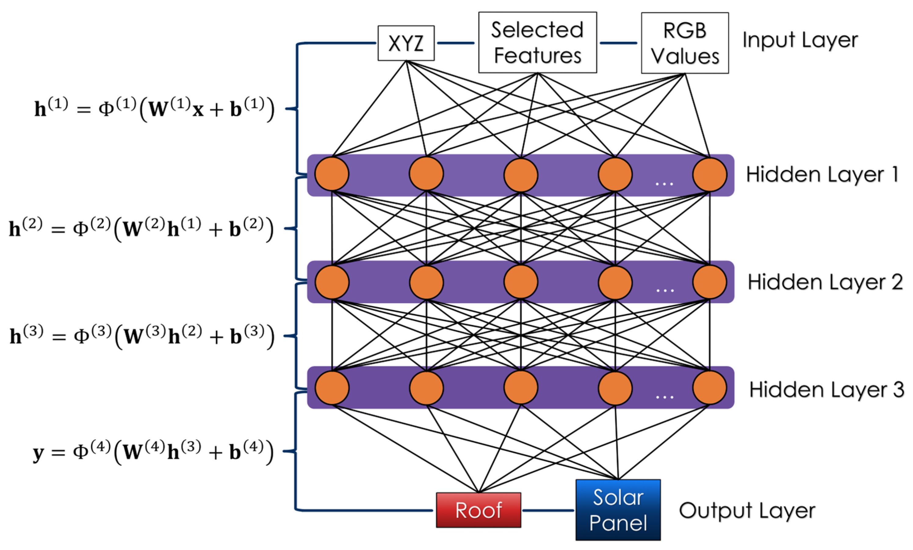
where $\mathbf{x}$ is the input feature vector consisting of spatial coordinates (X, Y, Z), selected geometric features, and RGB values, ${\mathbf{h}}^{\left(l\right)}$ is the activation vector of layer $l$, ${\mathbf{W}}^{\left(l\right)}$ is the weight matrix, ${\mathbf{b}}^{\left(l\right)}$ is the bias vector, and $\mathsf{\Phi }$ is the activation function for layer $l$, applied element-wise.

For our study, $\mathbf{y}$ is the output vector of the network, representing class predictions, either roof or solar panel.

ReLU has become the standard activation function in deep neural networks for its simplicity and strong performance [29]. Both Scikit-learn and PyTorch models in this study use ReLU activations in the hidden layers. The output layer applies sigmoid or softmax activation for Scikit-learn and PyTorch, respectively [30,31], producing class probabilities for binary classification (roof or solar panel).

Figure 6 illustrates the architecture of the MLP classifier used in this study, including the input features, hidden layers with neurons (each with their learned weights and biases), and the final predicted output classes.

Each row in the input table corresponds to a single point, with columns representing spatial coordinates (X, Y, Z), RGB values, selected geometric features, and a class label (0 for roof, 1 for solar panel). These input features are arranged as a matrix of shape $X\in R^{(\mathrm{N}\times \mathrm{F})}$ where $N$ (rows) represents each point in the dataset, and $F$ (columns) represents every associated feature [32].

2.4.1. MLP Configuration

Hyperparameter tuning was applied to improve classifier performance. This included adjustments to the hidden layers, neuron structure, and learning rate schedule. The refined architecture for both models used three hidden layers (100, 100, and 50 neurons in each). A summary of these parameters is provided in

Table 3. Parameters used for both models. Methods were replicated (where possible) to reduce bias and show fair comparison between frameworks.

Parameters	PyTorch Model	Scikit-Learn Model
Execution Mode	GPU	CPU
Architecture	MLP (3 hidden layers)	MLP (3 hidden layers)
Neuron Structure	100→100→50	100→100→50
Activation Function	ReLU	ReLU
Batch Normalisation	BatchNorm1d	Not available
Learning Rate Schedule	StepLR (Halved every 10 epochs)	Constant learning rate
Optimiser	Adam	Adam
Training Epochs	50	50
Data Split	70% Training 10% Validation 20% Testing
Number of Features	13 (UniSQ)/12 (Newcastle)	13 (UniSQ)/12 (Newcastle)
Batch Size	256	256
Average Training Time	~109 s (UniSQ)/~50 s (Newcastle)	~110 s (UniSQ)/~47 s (Newcastle)
Evaluation	Accuracy, Precision, Recall, F1 Score

.

2.4.2. Validation Strategy

Classifier performance was evaluated on the test set using accuracy, precision, recall, and F1 scores derived from the confusion matrix [3]. This helps to assess overall performance and the model’s ability to correctly identify minority classes (such as solar panels) in imbalanced datasets.

For solar panels as the positive class (class 1), the components of the confusion matrix are defined as:

• True Positive (TP): Solar panel points correctly classified as class 1.
• True Negative (TN): Roof points correctly classified as class 0.
• False Positive (FP): Roof points incorrectly classified as panels.
• False Negative (FN): Panel points incorrectly classified as roof.

From these components, performance can be calculated [33]:

$$Accuracy={\displaystyle \frac{TP+TN}{TP+FP+TN+FN}}$$

(20)

$$Precision={\displaystyle \frac{TP}{TP+FP}}$$

(21)

$$Recall={\displaystyle \frac{TP}{TP+FN}}$$

(22)

$$F_1 score=2 ·{\displaystyle \frac{Precision ·Recall}{Precision+Recall}}$$

(23)

These scores can range from 0 to 1, where 1 indicates perfect classification. While accuracy provides a general overview of model performance, it may be misleading in imbalanced datasets. Precision and recall offer more insight into model behaviour. In both datasets used in this study, roof points significantly outnumber panel points. Therefore, the F1 score, as the harmonic mean of precision and recall, provides a more balanced measure of performance for solar panel detection.

3. Results

This section presents results from the feature analyses and supervised classification experiments. First, we evaluate class separability using geometric and RGB features. Then, classification performance is reported for both datasets using PyTorch and Scikit-learn MLP models. Finally, we compare frameworks and summarise overall findings.

3.1. Feature Performance and Histogram Analysis

3.1.1. Geometric Features Histogram Analysis

With all geometric features defined and calculated using a consistent spherical neighbourhood for each dataset in CloudCompare, the next step is to assess their distribution across the two classes, roof and solar panel. This will be undertaken using a histogram analysis. A similar approach was used by Tarsha Kurdi et al. [2] to inspect geometric features across three classes: terrain, building, and vegetation. Likewise, Amakhchan et al. [10] analysed vegetation and terrain in both flat and mountainous areas. While the distinction between roof and panel surfaces is more subtle than between buildings and vegetation, the same method is applied here to evaluate the degree of class separation provided by each feature.

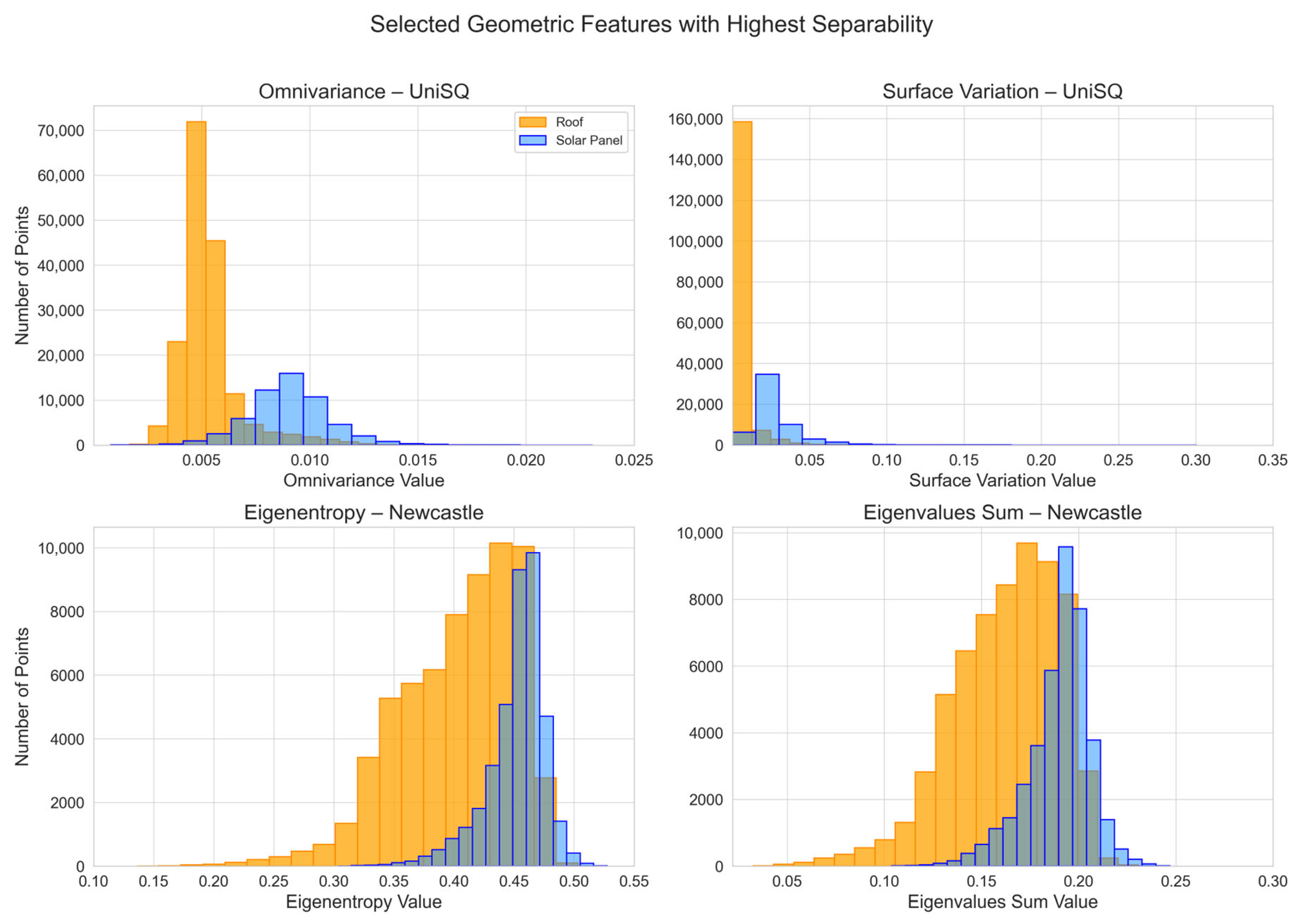
Each histogram represents the frequency distribution of a geometric feature, which is separated by class. This is supported by a statistical analysis, including histogram overlap and Kullback–Leibler (KL) divergence, to quantify how well each feature is distinguished between the two classes. Figure 7 highlights the best performing geometric features from each dataset.

3.1.2. RGB Channel Analysis

In addition to geometric descriptors, Red, Green, and Blue (RGB) channels were evaluated to determine their contribution to class separability. Figure 8 shows the histogram analysis for RGB values across both datasets.

For the UniSQ dataset, all three channels provided strong separation between roof and solar panel classes, with low overlaps and KL divergence values near or above 1.0. Consequently, red, green, and blue features were all retained for classification, as summarised in

Table 4. Selected RGB features for both datasets based on histogram analysis and KL divergence, highlighted in bold.

Dataset	Feature	Histogram Overlap	KL Divergence (Roof||Panel)	KL Divergence (Panel||Roof)	Acceptance
	Red	0.4	0.8	1.2	Yes
UniSQ	Green	0.4	0.9	1.1	Yes
	Blue	0.3	1.1	1.2	Yes
	Red	0.3	3.3	1.7	Yes
Newcastle	Green	0.5	1.6	0.8	Yes
	Blue	0.7	1.1	0.3	No

.

The Newcastle dataset showed greater variability. The red channel offered the clearest separation (overlap 0.3; KL divergence 3.3 and 1.7), the green channel was borderline but still useful (overlap 0.5; KL divergence 1.6 and 0.8), while the blue channel performed poorly (overlap 0.7; KL divergence 1.1 and 0.3) and was therefore discarded. These results are also reflected in Table 4.

Overall, the results demonstrate that spectral contributions are dataset dependent: UniSQ benefited from all three channels, while Newcastle relied primarily on the red channel, with green contributing moderately and blue adding little value.

3.2. Classification Performance

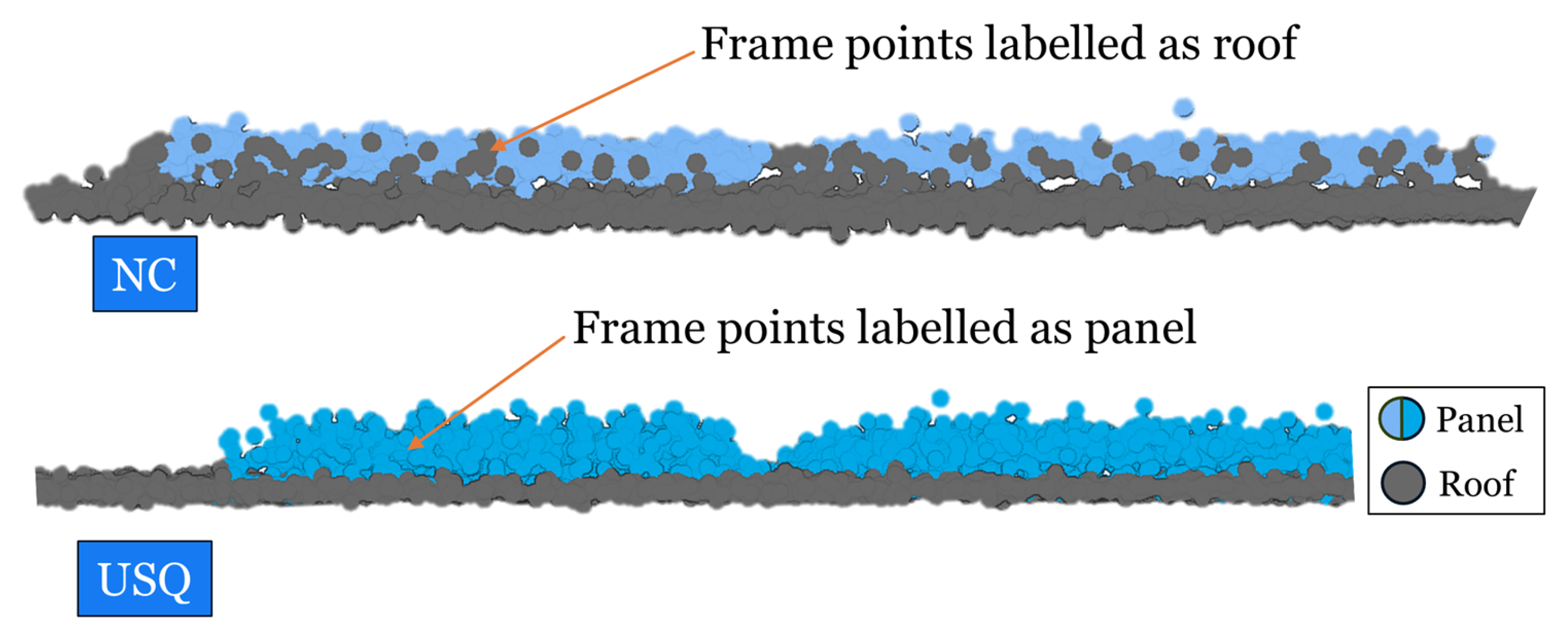
Each dataset was classified using a consistent MLP-based approach, but with differing preprocessing strategies. The UniSQ dataset underwent more meticulous cleaning, with solar panel points separated from roof points using RANSAC-based plane segmentation. Outer frame points were included as panel labels, as they coincided with the extracted plane. Noisy objects such as air conditioners and unrelated roof structures were manually removed.

In contrast, the Newcastle dataset was classified using reflectance values alone, with minimal cleaning or refinement. Frame points around solar panels were often classified as roof due to their proximity and similarity in geometry. Performance indicators, including accuracy scores and confusion matrices, are presented to evaluate the effectiveness of each approach.

3.2.1. Results—PyTorch and Scikit-Learn Models—UniSQ Dataset

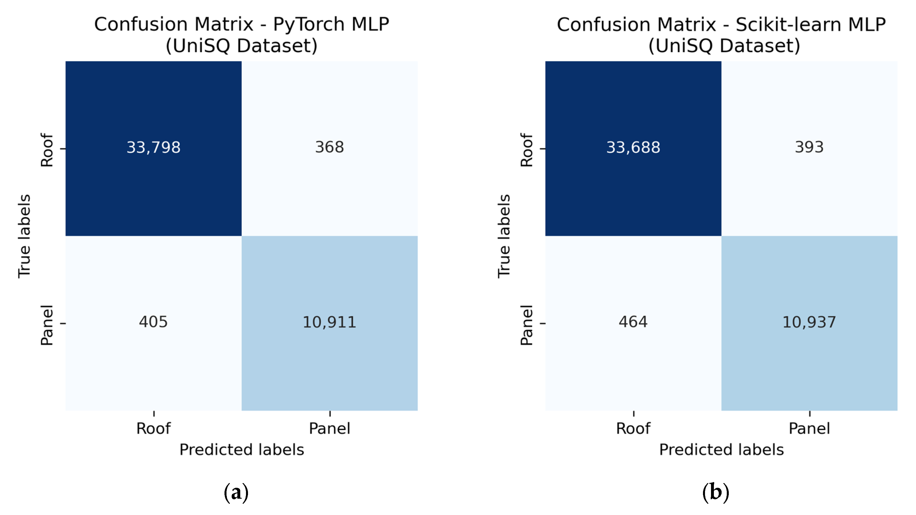
The UniSQ dataset contained 227,410 labelled points, which were split into 159,187 for training, 22,741 for validation, and 45,482 for testing. Both the PyTorch and Scikit-learn MLP models demonstrated strong classification performance. Each achieved a macro-average score of approximately 98% on the test set, indicating balanced performance across both classes. Final overall accuracy was approximately 98% for both models. This indicates they both generalised well to unseen data.

F1 scores for individual classes were 0.99 for roof and 0.96–0.97 for panel points, with PyTorch outperforming Scikit-learn by 0.01. These values confirm the model’s effectiveness, even with a moderate class imbalance. Notably, both models achieved high recall for class 1 (solar panels), meaning that very few panel points were mislabelled. Detailed test set performance is shown in

Table 5. Precision, recall and F1 scores for both PyTorch and Scikit-learn models on the UniSQ test set.

Class	Measure	PyTorch	Scikit-Learn
	Precision	0.99	0.99
Roof (0)	Recall	0.99	0.99
	F1-Score	0.99	0.99
	Precision	0.97	0.97
Solar Panel (1)	Recall	0.96	0.96
	F1-Score	0.97	0.96

.

The confusion matrices shown in Figure 9 show classifier performance across the two classes, roof (class 0) and solar panel (class 1), using the TP, TN, FP, and FN definitions. PyTorch achieved fewer false positives and negatives compared to Scikit-learn. Conversely, Scikit-learn had more true positives but more misclassifications overall. PyTorch showed slightly stronger performance for classification consistency, mostly for roof points. Overall, both models generalised well and handled class imbalance effectively.

3.2.2. Results—PyTorch and Scikit-Learn Models—Newcastle Dataset

The Newcastle dataset contained 103,087 labelled points, split into 72,160 for training, 10,309 for validation, and 20,618 for testing. While not as strong as the UniSQ results, both models still achieved solid performance, with a macro-average score of approximately 94%, indicating reasonably balanced classification across both classes. Final overall accuracy was 95% for the PyTorch model and 94% for the Scikit-learn model, showing that both models performed well.

Results were mostly consistent across the two models. PyTorch performed better in recall and F1 score for the roof class. Precision and F1 score were slightly higher for panel points in the PyTorch model, by approximately 0.01. A detailed analysis is shown in

Table 6. Precision, recall and F1 scores for both PyTorch and Scikit-learn models on the Newcastle test set.

Class	Measure	PyTorch	Scikit-Learn
	Precision	0.97	0.97
Roof (0)	Recall	0.95	0.93
	F1-Score	0.96	0.95
	Precision	0.91	0.90
Solar Panel (1)	Recall	0.95	0.95
	F1-Score	0.93	0.92

.

The confusion matrices shown in Figure 10 show classifier performance across the two classes, roof (class 0) and solar panel (class 1), using the TP, TN, FP, and FN definitions. Both models performed similarly overall, with very close false negative counts. PyTorch achieved fewer false positives, notably for roof classification. Although Scikit-learn showed a high number of correctly classified panel points, this was due to a higher number of panel samples in the test set, caused by differences in how each model split data, even when using the same random seed. Overall, both models handled the dataset well and proved reliable.

Overall, PyTorch showed slightly stronger classification consistency and recall, particularly for panel detection, while Scikit-learn remained competitive. Differences were marginal given dataset size. Both frameworks generalised well across the two datasets and proved robust for roof vs. solar panel classification tasks.

4. Discussion

4.1. Dataset Quality

The UniSQ dataset featured large, uniform roof sections, which allowed RANSAC-based separation of panels from roof structures. However, this also resulted in panel frame points being included as part of the panel class. Conversely, the Newcastle dataset was labelled using the reflectance attribute, which excluded the frame and treated those points as the roof. While more efficient, reflectance-based labelling may have contributed to closer classification boundaries, as many roof and panel points occupied similar spatial planes (X, Y, Z). This can be seen in Figure 11. Despite the variation in roof structures and panel arrangements in Newcastle, reflectance-based labelling proved to be a faster alternative.

It is also worth noting that the UniSQ dataset contained industrial-sized panels, which were consistently spaced and elevated above the roof surface. Due to the beam width and angled incidence of airborne LiDAR, returns near panel edges may be sparse or mixed. These mixed returns can originate from the panel, the supporting surface or the underlying roof, depending on the incidence angle and material properties. This has been observed in previous studies, where accuracy is affected by mixed returns near object boundaries [34].

Figure 12 shows a section of roof from the UniSQ test set, where predicted panel and roof points are shown alongside misclassified points in red. These misclassified points generally cluster around the solar panel edges and roof transitions, consistent with the expectation that geometry is more ambiguous in these areas, which can reduce the reliability of geometric features such as omnivariance or surface variation. This visually reinforces how edge complexity and return inconsistency influence classification accuracy, even in a thoroughly labelled dataset.

4.2. Model Performance and Feature Relevance

Both classifiers demonstrated strong performance overall, with PyTorch consistently achieving slightly higher accuracy across both datasets. Differences in feature importance, however, became more apparent when RGB channels were removed, especially for the Newcastle dataset, which lacked strong class separation based purely on selected geometric features.

For UniSQ, removing RGB values did not have much of an impact, with Pytorch’s accuracy only dropping by 0.2% (from 98.3% to 98.1%). This suggests that the model relies mainly on geometric features. This may be due to the consistent panel structures and clearer segmentation achieved through RANSAC.

Notably, removing the red and green (R and G) values from the Newcastle dataset had a significant impact on accuracy, particularly for the Scikit-learn model, a drop of approximately 4% (from 93.8% to 89.7%). Also of note was that Scikit-learn’s false negative rate more than doubled without red and green, showing reduced ability to differentiate panels from the roof. This indicates that red and green channels compensated for the weaker geometric features.

Comparing these results to Tarsha Kurdi et al. [2] and Amakhchan et al. [10], both studies used an MLP classifier, achieving accuracy scores of approximately 98%. Amakhchan et al. [10] compared terrain and vegetation classes in flat and mountainous areas, while Tarsha Kurdi et al. [2] classified building, vegetation, and terrain in urban areas. These results demonstrate that MLP-based models can achieve high accuracy scores across a range of LiDAR classification tasks. In this study, despite the greater challenge of differentiating rooftop solar panels from roof surfaces, both MLP classifiers scored just above 98% accuracy on the UniSQ dataset.

These results, shown in

Table 7. For the UniSQ dataset, removing RGB reduces accuracy by <0.3%, indicating geometric features alone were sufficient.

Measure (UniSQ)	PyTorch	PyTorch (No RGB)	Difference	Scikit-Learn	Scikit-Learn (No RGB)	Difference
True Positives (TP)	10,911	10,937	26	10,831	10,833	2
False Negatives (FN)	405	464	59	485	568	83
True Negatives (TN)	33,798	33,688	110	33,792	33,665	127
False Positives (FP)	368	393	25	374	416	42
Accuracy (%)	98.30	98.12	−0.18	98.11	97.84	−0.27

and

Table 8. For the Newcastle dataset, accuracy dropped 3–4% without red and green values, indicating that these were needed due to weaker geometric separation.

Measure (Newcastle)	PyTorch	PyTorch (No Red/Green)	Difference	Scikit-Learn	Scikit-Learn (No Red/Green)	Difference
True Positives (TP)	7412	7388	24	7481	7037	444
False Negatives (FN)	415	439	24	422	866	444
True Negatives (TN)	12,095	11,498	597	11,864	11,470	394
False Positives (FP)	696	1293	597	851	1245	394
Accuracy (%)	94.61	91.60	−3.01	93.83	89.76	−4.06

, confirm that feature selection must be tailored to the quality and characteristics of the LiDAR data. While geometric features can be sufficient in structured datasets, spectral attributes such as RGB become equally important when rooftop structures and panel arrangements are more varied or complex.

5. Conclusions

This study explored the supervised classification of solar panels and roof structures using LiDAR point cloud data from two different datasets, UniSQ and Newcastle. Geometric and RGB features were selected through histogram analysis and KL divergence. This gave early insight into how well the MLP models, implemented using PyTorch and Scikit-learn, would perform across different datasets.

The UniSQ dataset, with clear panel definition achieved through RANSAC, demonstrated excellent performance with minimal reliance on RGB features. Comparatively, the Newcastle dataset had a greater variety of rooftop structures and solar panel arrangements that showed greater dependency on spectral attributes, especially red and green channels. Where geometric feature separation was weaker, these spectral inputs effectively supplemented the model’s ability to distinguish panels from roofs.

Across both datasets, PyTorch showed slightly higher performance (0.2% and 0.8% in accuracy for UniSQ and Newcastle, respectively), possibly due to model features such as batch normalisation, learning rate scheduling (StepLR), and GPU acceleration. Although training times remained consistent between both models (~110 s for UniSQ and ~50 s for Newcastle), future work with larger datasets may reveal performance differences between GPU-based (PyTorch) and CPU-based (Scikit-learn) implementations. This comparison across PyTorch and Scikit-learn implementations is intended as a robustness check rather than a primary contribution

The results highlight the importance of feature selection. No single configuration performed optimally across both datasets. Histogram analysis and KL divergence were essential tools for understanding feature behaviour and directing the selection process. For more uniform rooftop and panel configurations like UniSQ, geometric features may suffice. However, for Newcastle, with varying roof structures and panel arrangements, RGB analysis proved to be a critical measure in the feature selection process.

Reflectance proved to be a fast and practical labelling approach that offered clear class separation with minimal preprocessing, a useful tactic when RANSAC was more difficult to implement. However, using RANSAC, where possible, can lead to a more structured labelling outcome. This approach, in conjunction with removing noise in early preprocessing stages, can help with maintaining clear separation between panels and rooftop sections.

Overall, this work demonstrates that thorough data labelling, careful feature selection, and iterative model tuning make the classification of solar panels using LiDAR data achievable across varied and imperfect datasets. Notably, most classification errors were observed along panel edges and roof transitions, a pattern recognised across both test sets.

Future Research

While this study has demonstrated that LiDAR-derived features can achieve high classification accuracy for rooftop solar panels, several important areas remain open for future research. One key limitation is that the current work focused on classification within pre-segmented rooftop areas. Although this reflects a common operational workflow where roof polygons are provided by councils or utilities, extending the methodology to full scene-level detection from raw point clouds is a valuable direction. Such an approach would pose additional challenges, including background clutter, non-panel rooftops, and stronger class imbalance, but it would provide a more realistic and comprehensive framework for large-scale deployment. Embedding the classifier within a two-stage pipeline, where roof segmentation is followed by panel classification, may help address these challenges, though headline accuracy is expected to decrease under this more difficult setting.

Another important area for development is cross-modal comparisons and fusion. While this study concentrated on LiDAR point clouds and geometric features, prior work has shown that image-based object detection, such as YOLO applied to aerial or satellite imagery, can achieve high performance. Pena Pereira et al. [35], for example, used RGB and Near-Infrared data across 171 building types, with over 12,500 panels, and reported F1 scores exceeding 90 percent. Their findings also highlighted that adding height information would further enrich the training data, suggesting that hybrid approaches that integrate spectral and geometric information could outperform single-modality systems. Future work should therefore explore how LiDAR features can be combined with spectral data from UAV or satellite imagery to improve generalisation across diverse urban environments.

In addition to expanding sensing modalities, future studies should consider more robust feature selection and broader model comparisons. In this study, histogram overlap and KL divergence values were applied as heuristic guides supported by visual inspection, but these thresholds may not generalise across datasets. Larger and more diverse datasets would allow for systematic ranking methods such as SHAP values or mutual information, which could provide site-agnostic feature importance. Similarly, while this work focused on MLPs as a proof of concept, evaluating additional baseline models such as Random Forest, XGBoost, and point-cloud deep learning methods like PointNet++ would provide stronger benchmarking. Statistical significance testing, for example, using paired t-tests or McNemar’s test, should also be incorporated in such comparative analyses.

Reflectance, which played a major role in dataset preparation for separating panel surfaces from roofs, also warrants further investigation as a direct classification feature. Its integration alongside geometric and RGB features may enhance performance. Incorporating additional rooftop structures such as air conditioners could extend the task from binary classification to multi-class models that better capture the variety of rooftop objects. Furthermore, class imbalance remains a challenge, as panel points were far sparser than roof points in both datasets. Oversampling strategies, synthetic data augmentation, or weighted loss functions may improve robustness, particularly in large heterogeneous urban scenes.

Finally, expanding the scope of solar panel detection from individual rooftops to city-wide applications represents an important practical goal. Previous studies have mainly focused on estimating rooftop potential [36], but relatively few have attempted to count already installed panels.

In summary, future research should aim to move from rooftop-level classification towards scene-level detection, integrate LiDAR with complementary spectral data, adopt more generalisable feature ranking and modelling approaches, incorporate reflectance and rooftop structures as classification features, address class imbalance through advanced sampling strategies, and develop scalable methods for city-wide panel counting. Together, these directions will help advance solar panel mapping from proof-of-concept experiments to robust, generalisable, and operational tools for energy planning.

References

1. McTegg, S.J.; Tarsha Kurdi, F.; Simmons, S.; Gharineiat, Z. Comparative approach of unmanned aerial vehicle restrictions in controlled airspaces. Remote Sens. 2022, 14, 822. [Google Scholar] [CrossRef]
2. Tarsha Kurdi, F.; Amakhchan, W.; Gharineiat, Z.; Boulaassal, H.; El Kharki, O. Contribution of geometric feature analysis for deep learning classification algorithms of urban LiDAR data. Sensors 2023, 23, 7360. [Google Scholar] [CrossRef] [PubMed]
3. Sharma, M.; Garg, R.D. Building footprint extraction from aerial photogrammetric point cloud data using its geometric features. J. Build. Eng. 2023, 76, 107387. [Google Scholar] [CrossRef]
4. Pellerin Le Bas, X.; Froideval, L.; Mouko, A.; Conessa, C.; Benoit, L.; Perez, L. A New Open-Source Software to Help Design Models for Automatic 3D Point Cloud Classification in Coastal Studies. Remote Sens. 2024, 16, 2891. [Google Scholar] [CrossRef]
5. Hosseini, M.; Bagheri, H. Improving the resolution of solar energy potential maps derived from global DSMs for rooftop solar panel placement using deep learning. Heliyon 2025, 11, e41193. [Google Scholar] [CrossRef]
6. Yadav, Y.; Harshit; Kushwaha, S.K.P.; Zlatanova, S.; Boccardo, P.; Jain, K. Assessing Photo-Voltaic Potential in Urban Environments: A Comparative Study between Aerial Photogrammetry and LiDAR Technologies. Int. Arch. Photogramm. Remote Sens. Spat. Inf. Sci. 2024, 48, 533–539. [Google Scholar] [CrossRef]
7. Jiang, H.; Yao, L.; Lu, N.; Qin, J.; Liu, T.; Liu, Y.; Zhou, C. Multi-resolution dataset for photovoltaic panel segmentation from satellite and aerial imagery. Earth Syst. Sci. Data Discuss. 2021, 13, 5389–5401. [Google Scholar] [CrossRef]
8. Clark, C.N.; Pacifici, F. A solar panel dataset of very high resolution satellite imagery to support the Sustainable Development Goals. Sci. Data 2023, 10, 636. [Google Scholar] [CrossRef]
9. Duran, Z.; Ozcan, K.; Atik, M.E. Classification of photogrammetric and airborne lidar point clouds using machine learning algorithms. Drones 2021, 5, 104. [Google Scholar] [CrossRef]
10. Amakhchan, W.; Kurdi, F.T.; Gharineiat, Z.; Boulaassal, H.; El Kharki, O. Classification of Forest LiDAR Data Using Deep Learning Pipeline Algorithm and Geometric Feature Analysis. Int. J. Environ. Sci. Nat. Resour. 2023, 32, 556340. [Google Scholar] [CrossRef]
11. Kushwaha, S.; Harshit; Jain, K. Solar Roof Panel Extraction from UAV Photogrammetric Point Cloud. In Proceedings of the International Conference on Unmanned Aerial System in Geomatics, Roorkee, India, 2–4 April 2021; pp. 173–185. [Google Scholar]
12. Tarsha-Kurdi, F.; Landes, T.; Grussenmeyer, P. Extended RANSAC algorithm for automatic detection of building roof planes from LiDAR data. Photogramm. J. Finl. 2008, 21, 97–109. [Google Scholar]
13. RIEGL. LAS Extrabytes Implementation in RIEGL Software; RIEGL Laser Measurement Systems GmbH: Horn, Austria, 2019; p. 12. [Google Scholar]
14. Weinmann, M.; Jutzi, B.; Mallet, C. Feature relevance assessment for the semantic interpretation of 3D point cloud data. ISPRS Ann. Photogramm. Remote Sens. Spat. Inf. Sci. 2013, 2, 313–318. [Google Scholar] [CrossRef]
15. Hackel, T.; Wegner, J.D.; Schindler, K. Contour detection in unstructured 3D point clouds. In Proceedings of the IEEE Conference on Computer Vision and Pattern Recognition, Las Vegas, NV, USA, 27–30 June 2016; pp. 1610–1618. [Google Scholar]
16. Thomas, H.; Goulette, F.; Deschaud, J.-E.; Marcotegui, B.; LeGall, Y. Semantic classification of 3D point clouds with multiscale spherical neighborhoods. In Proceedings of the 2018 International Conference on 3D Vision (3DV), Verona, Italy, 5–8 September 2018; pp. 390–398. [Google Scholar]
17. Demantké, J.; Vallet, B.; Paparoditis, N. Streamed vertical rectangle detection in terrestrial laser scans for facade database production. ISPRS Ann. Photogramm. Remote Sens. Spat. Inf. Sci. 2012, 1, 99–104. [Google Scholar] [CrossRef]
18. CloudCompare. Roughness. Available online: https://www.cloudcompare.org/doc/wiki/index.php/Roughness (accessed on 27 March 2025).
19. Swain, M.J.; Ballard, D.H. Color indexing. Int. J. Comput. Vis. 1991, 7, 11–32. [Google Scholar] [CrossRef]
20. Kullback, S.; Leibler, R.A. On information and sufficiency. Ann. Math. Stat. 1951, 22, 79–86. [Google Scholar] [CrossRef]
21. Dehbi, Y.; Koppers, S.; Plümer, L. Probability Density Based Classification and Reconstruction of Roof Structures from 3D Point Clouds. Int. Arch. Photogramm. Remote Sens. Spat. Inf. Sci. 2019, 42, 177–184. [Google Scholar] [CrossRef]
22. Cardoso, A.; Jurado-Rodríguez, D.; López, A.; Ramos, M.I.; Jurado, J.M. Automated detection and tracking of photovoltaic modules from 3D remote sensing data. Appl. Energy 2024, 367, 123242. [Google Scholar] [CrossRef]
23. Pedregosa, F.; Varoquaux, G.; Gramfort, A.; Michel, V.; Thirion, B.; Grisel, O.; Blondel, M.; Prettenhofer, P.; Weiss, R.; Dubourg, V. Scikit-learn: Machine learning in Python. J. Mach. Learn. Res. 2011, 12, 2825–2830. [Google Scholar]
24. Scikit-Learn. Neural Networks—Supervised. Available online: https://scikit-learn.org/stable/modules/neural_networks_supervised.html (accessed on 6 May 2025).
25. Paszke, A. Pytorch: An imperative style, high-performance deep learning library. arXiv 2019, arXiv:1912.01703. [Google Scholar]
26. Amakhchan, W.; Tarsha Kurdi, F.; Gharineiat, Z.; Boulaassal, H.; El Kharki, O. Automatic filtering of LiDAR building point cloud using multilayer perceptron Neuron Network. In Proceedings of the 3rd International Conference on Big Data and Machine Learning (BML22’), Istanbul, Turkey, 23–24 May 2022. [Google Scholar]
27. Goodfellow, I.; Bengio, Y.; Courville, A.M.I.T. Deep Learning; MIT Press: Cambridge, MA, USA, 2016. [Google Scholar]
28. Grosse, R. Multilayer Perceptrons (Lecture 5). Available online: https://www.cs.toronto.edu/~rgrosse/courses/csc321_2018/readings/L05%20Multilayer%20Perceptrons.pdf (accessed on 20 June 2025).
29. Nair, V.; Hinton, G.E. Rectified linear units improve restricted boltzmann machines. In Proceedings of the 27th International Conference on Machine Learning (ICML-10), Haifa, Israel, 21–24 June 2010; pp. 807–814. [Google Scholar]
30. PyTorch-Developers. CrossEntropyLoss-Pytorch Documentation. Available online: https://docs.pytorch.org/docs/stable/generated/torch.nn.CrossEntropyLoss.html (accessed on 20 June 2025).
31. Scikit-Learn-Developers. MLPClassifier—Multi-Layer Perceptron Classifier. Available online: https://scikit-learn.org/stable/modules/generated/sklearn.neural_network.MLPClassifier.html (accessed on 20 June 2025).
32. Wu, H.; Shen, G.; Lin, X.; Li, M.; Zhang, B.; Li, C.Z. Screening patents of ICT in construction using deep learning and NLP techniques. Eng. Constr. Archit. Manag. 2020, 27, 1891–1912. [Google Scholar] [CrossRef]
33. Li Persson, L. Automatic Processing of LiDAR Point Cloud Data Captured by Drones; Digitala Vetenskapliga Arkivet (DiVA): Uppsala, Sweden, 2023. [Google Scholar]
34. Zhou, K.; Lindenbergh, R.; Gorte, B.; Zlatanova, S. LiDAR-guided dense matching for detecting changes and updating of buildings in Airborne LiDAR data. ISPRS J. Photogramm. Remote Sens. 2020, 162, 200–213. [Google Scholar] [CrossRef]
35. Pena Pereira, S.; Rafiee, A.; Lhermitte, S. Automated rooftop solar panel detection through Convolutional Neural Networks. Can. J. Remote Sens. 2024, 50, 2363236. [Google Scholar] [CrossRef]
36. Tiwari, A.; Meir, I.A.; Karnieli, A. Object-based image procedures for assessing the solar energy photovoltaic potential of heterogeneous rooftops using airborne LiDAR and orthophoto. Remote Sens. 2020, 12, 223. [Google Scholar] [CrossRef]
Figure 1. Elevated panel classification process for A block in the UniSQ dataset, RANSAC has effectively separated panels from the roof (green), which allows for classification of roof (blue) and panels (red).
Remotesensing 17 03389 g001
Figure 2. Flat panel (red) and roof (green) classification process for D block in the UniSQ dataset.
Remotesensing 17 03389 g002
Figure 3. Segmented roofs (red) and panels (blue) from the Newcastle dataset using the reflectance scalar field for classification.
Remotesensing 17 03389 g003
Figure 4. Reflectance-based classification using CloudCompare. Reflectance scale shown in dB. Lower values (−19.8 dB to −10 dB) correspond to solar panel surfaces, while higher values (−10 dB to −2.2 dB) align with rooftop returns.
Remotesensing 17 03389 g004
Figure 5. Workflow for supervised classification using an MLP model.
Remotesensing 17 03389 g005
Figure 6. Architecture of the MLP classifier used in this study. The input features, x (Spatial coordinates, selected geometric features, and RGB values) are passed through three hidden layers with ReLU as the activation function. The final output predictions, y , are either roof or solar panel.
Remotesensing 17 03389 g006
Figure 7. Distributions of the best performing geometric features. Omnivariance and surface variation showed the strongest class separation for the UniSQ dataset (top row). Eigenentropy and Sum of Eigenvalues were the most effective for the Newcastle dataset (bottom row).
Remotesensing 17 03389 g007
Figure 8. Distributions of red (top), green (middle) and blue (bottom) channel values for roof and solar panel classes in UniSQ and Newcastle datasets.
Remotesensing 17 03389 g008
Figure 9. Confusion matrices for PyTorch (a) and Scikit-learn (b) classifiers on the UniSQ test set. Performance metrics are provided in Table 5.
Remotesensing 17 03389 g009
Figure 10. Confusion matrices for PyTorch (a) and Scikit-learn (b) classifiers on the Newcastle test set. Performance metrics are provided in Table 6.
Remotesensing 17 03389 g010
Figure 11. Side view of a roof section from both datasets, highlighting differences in panel labelling. In the Newcastle dataset, reflectance captured only the inner panel points, with frame points labelled as roof. By comparison, the UniSQ dataset used RANSAC to isolate the roof plane, assigning both panel and frame points to the panel class.
Remotesensing 17 03389 g011
Figure 12. Top-down view of a section of elevated panels on A block, from the UniSQ test set (20%). Misclassified points (in red) are primarily concentrated around solar panel edges and roof transitions. This pattern was also observed in both UniSQ and Newcastle test sets, showing where geometric ambiguity led to reduced classification accuracy.
Remotesensing 17 03389 g012