Spatiotemporal Analysis of Vineyard Dynamics: UAS-Based Monitoring at the Individual Vine Scale

Highlights

This study introduces a framework for monitoring vineyards at the level of individual vines. Using synchronized UAS-based RGB and multispectral imagery, photogramme-try, and an object-based image analysis (OBIA), vines are detected directly from 3D point clouds without training data. The method creates canopy-only masks for each plant and computes per-vine NDRE at key phenological stages (flowering, veraison, harvest). Spatial statistics (LISA) reveal coherent high- and low-vigour zones and sin-gle-vine outliers. A strong NDRE–yield relationship confirms that the mapped vigour reflects real productivity, enabling targeted, site-specific management.

What are the main findings?

• Individual vines were detected from UAS-based 3D point clouds achieving a 10.7 cm mean Euclidean distance to reference measurements; OBIA yielded canopy masks for unbiased NDRE values of individual vines.
• Canopy-only, per-vine NDRE across key phenological phases showed strong spatial autocorrelation; LISA exposed stable zones of high and low vigour and outliers.

What is the implication of the main finding?

• Managers can target interventions at plant scale—identifying early stress hotspots and isolated problem vines before spread.
• The workflow is transferable and operational for routine vine monitoring, supporting site-specific decisions and yield/resource optimization.

Abstract

The rapid and reliable acquisition of canopy-related metrics is essential for improving decision support in viticultural management, particularly when monitoring individual vines for targeted interventions. This study presents a spatially explicit workflow that integrates Uncrewed Aerial System (UAS) imagery, 3D point-cloud analysis, and Object-Based Image Analysis (OBIA) to detect and monitor individual grapevines throughout the growing season. Vines are identified directly from 3D point clouds without the need for prior training data or predefined row structures, achieving a mean Euclidean distance of 10.7 cm to the reference points. The OBIA framework segments vine vegetation based on spectral and geometric features without requiring pre-clipping or manual masking. All non-vine elements—including soil, grass, and infrastructure—are automatically excluded, and detailed canopy masks are created for each plant. Vegetation indices are computed exclusively from vine canopy objects, ensuring that soil signals and internal canopy gaps do not bias the results. This enables accurate per-vine assessment of vigour. NDRE values were calculated at three phenological stages—flowering, veraison, and harvest—and analyzed using Local Indicators of Spatial Association (LISA) to detect spatial clusters and outliers. In contrast to value-based clustering methods, LISA accounts for spatial continuity and neighborhood effects, allowing the detection of stable low-vigour zones, expanding high-vigour clusters, and early identification of isolated stressed vines. A strong correlation (R² = 0.73) between per-vine NDRE values and actual yield demonstrates that NDRE-derived vigour reliably reflects vine productivity. The method provides a transferable, data-driven framework for site-specific vineyard management, enabling timely interventions at the individual plant level before stress propagates spatially.

1. Introduction

A subdomain of precision agriculture is precision viticulture (PV). PV is a management strategy that uses remote sensing, statistical analysis, and computer vision to monitor spatial and temporal variability in vineyards, particularly in relation to vine canopy architecture, agricultural production, and vine health [1,2]. One of its main goals is to support location-specific management decisions for each vineyard entity [3].

Remote sensing techniques are employed in precision agriculture for tasks like yield estimation [4,5] or plant segmentation [6,7]. A wide range of technologies are used to collect data on plant architecture, condition, climate, and soil, enabling decision support in viticulture through the analysis of spatiotemporal data [8]. Satellite imagery is commonly used in PV [9]. Depending on their spatial resolution, satellite images can be used for management at various scales. Their typically coarser resolution generally limits applications to plot-level analysis, where distinguishing between rows or individual plants is not feasible [10].

Uncrewed Aerial Systems (UAS), equipped with multispectral, high-resolution RGB, and thermal infrared sensors enhance vineyard monitoring through their high spatial, temporal, and spectral resolution capabilities [11]. The use of multispectral sensors enables the calculation of different vegetation indices (VI) that correlate to chlorophyll content within the leaves, nitrogen concentration, and the plants water status [10]. Healthy vegetation shows increased reflectance in the near-infrared spectrum and increased absorption in the RedEdge band. These spectral features support the detection and analysis of vegetation objects [12]. Spectral vegetation indices can be used to monitor changes within a vineyard ecosystem and to identify the vegetative and reproductive growth at different phenological stages. Lorenz et al. [13] structured the phenological stages of grapevines using the modified Eichhorn–Lorenz (EL) system. This system divides the vine’s vegetative cycle into 47 EL stages, each corresponding to a specific phenological phase. These stages are further grouped into major phases. For this project, spatial data of the following stages were collected: EL 4 (budburst), EL 23 (flowering), EL 35 (veraison), and EL 38 (harvest).

Ferro et al. [14] demonstrated a strong correlation between NDVI and NDRE with vine yield, reporting correlation coefficients of r = 0.8 and r = 0.72, respectively. Geostatistical analysis using VIs to model spatial variability supports improved vineyard management [14]. Since soil pixels can significantly influence VI values, it is necessary to perform monitoring that excludes non-canopy elements in multispectral datasets and focuses on target-species segmentation [15].

Vineyard row segmentation is performed using different methodologies. It is carried out by either pixel-based or object-based frameworks [8,16]. OBIA groups adjacent pixels with similar value ranges into objects and integrates topological, spectral, and spatial information for classification [17]. OBIA frameworks can incorporate supervised classifiers like Support Vector Machines (SVM) and Random Forest (RF) for canopy segmentation [18].

Kerkech et al. [19] developed a UAV-based method for detecting Mildew disease in vineyards, combining multispectral imaging and deep learning segmentation. Their approach integrated visible and infrared imagery through an optimized, non-rigid image registration process to align data from dual sensors. Using the SegNet deep learning architecture, they segmented images into classes such as healthy, symptomatic, ground, and shadow, achieving over 90% accuracy at the vine level. Although explicit plant geolocation was not provided, disease detection was performed at the plant scale using a patch-based method aligned with average vine size. The position of individual vines is outlined by many studies in the domain of precision viticulture [20,21]. Gavrilović et al. [3] detected individual vines by using YOLO as a deep learning algorithm where the shadow cast of the vine trees is detected. The method delivered sufficient results but is dependent on weather, daytime, and general location of the vineyard as shadowed vine blocks are difficult to monitor. In the presented study, grapevines are detected directly from a 3D point cloud without requiring training data or site-specific priors, and their positions are georeferenced in a projected coordinate system. OBIA is used to segment vine rows without pre-masking or excluding other land cover classes. The framework identifies vine vegetation based on geometric and spectral features. Individual vine locations are then used to generate detailed canopy masks, allowing vegetation indices to be calculated for each vine while excluding soil and inter-row vegetation signals.

Management zone delimitation in vineyards improves productivity and enables more efficient resource use through targeted practices applied to homogeneous zones [22]. Numerous methods were developed to measure plant variability and delineate homogeneous areas, with unsupervised clustering methods like K-means being widely used [23]. However, as vine diseases often spread spatially from plant to plant, incorporating spatial arrangement is valuable for health assessment.

Some studies perform vine canopy detection using height-based filtering from canopy height models, assuming that only grapevine vegetation is present in the scene [24,25]. However, height alone cannot reliably distinguish between vegetation species when the canopy extent is comparable between types. Ferro et al. [8] reviewed canopy detection methods, including mask R-CNN, U-Net, OBIA, and unsupervised techniques. While deep learning models showed superior performance, they required extensive training data. When vine canopies are accurately segmented, spectral information can be derived from isolated vine objects, reducing contamination from surrounding pixels. Prior studies mapped vineyard variability and defined homogeneous zones at the subplot level or through manual vine delineation [26,27].

This study introduces a workflow for vine-level monitoring that combines 3D point-cloud analysis, object-based image analysis (OBIA), and spatial statistics to overcome some limitations of existing approaches. Unlike methods that rely on shadow detection and are constrained by lighting conditions, vine locations are extracted directly from the 3D structure of the plants, independent of weather or sun angle and without the necessity of training data. The OBIA framework operates without the need for prior masking or row clipping and segments vine vegetation based solely on geometric and spectral characteristics, allowing it to generalize across different vineyard configurations. From the identified vine positions, individual canopy masks are generated, enabling the calculation of vegetation indices that represent the full canopy extent rather than relying on interpolated raster values. To analyze spatial and temporal patterns of vine vigour, Local Indicators of Spatial Association (LISA) is applied across three phenological stages. In contrast to clustering methods such as K-means, this spatially explicit approach captures both coherent vigour zones and spatial outliers, allowing for the identification of persistent stress areas and isolated anomalies where a problem area may form. The resulting analysis provides a robust basis for targeted vineyard management and supports early intervention at the individual plant level before stress propagates across zones.

2. Materials and Methods

2.1. Study Site

The study site, depicted in Figure 1, is situated in Carinthia, Austria, covering a 0.7 ha vineyard on a south/west-facing slope with an average incline of 17.4° at an elevation of approximately 750 m. The region is characterized by a temperate alpine climate with summer highs around 34 °C and −10 °C as the lowest winter temperatures. Since 2012, this vineyard is home to 1063 vines planted with an average spacing of 1 m. In the vineyard, white and red wine varieties, primarily ‘Bianca,’ ‘Regent,’ and ‘Jura’ are cultivated. The vines are managed without irrigation, with lime applied to enhance nutrient availability, and no chemical pesticides or fertilizers are used.

2.2. UAS Image Acquisition

The UAS DJI M350 RTK (SZ DJI Technology Co., Ltd., Shenzhen, Guangdong, China), equipped with two sensors, was employed to acquire the data (Figure 2). Very high-resolution RGB images were captured using DJI’s P1 RGB full-frame sensor, which provides a spatial resolution of 45 megapixels and a raw image size of 8192 × 5460 pixels. Multispectral images were obtained using the Micasense RedEdge-Dual sensor (Micasense Inc., Seattle, WA, USA). This multispectral sensor records data across 10 spectral bands with a spatial resolution of 7 cm. The spectral bands utilized in this study are Blue (475 nm), Green (560 nm), and Red (668 nm) in the visible spectrum as well as Red Edge (717 nm) and Near Infrared (NIR) (840 nm). The multispectral sensor was calibrated using the reference panels provided with the sensor both before and after the flights, following the protocol as described by Daniels et al. [28]. Five field survey campaigns were executed from September 2022 to October 2023 covering a full vegetative cycle and key phenological phases (budburst, flowering, veraison, and harvest). The exact dates of survey are shown in

Table 1. Survey dates and the phenological stages of vines and the respective GCP errors.

Date	Phenological Stage	GCP Error
23 September 2022	Harvest	1.5 cm
8 April 2023	Budburst	2.4 cm
14 July 2023	Flowering	3.0 cm
16 August 2023	Veraison	1.8 cm
6 October 2023	Harvest	1.6 cm

. The data was georeferenced using 8 Ground Control Points (GCP). The GCPs were measured with the Leica Differential GPS GS16 (Leica Geosystems, Heerburg, Switzerland) with RTK correction.

The UAS missions were conducted autonomously, following a predefined cross-grid flight pattern. Both the multispectral and RGB sensors were mounted on the M350 simultaneously, with synchronized camera triggering. This setup enabled the simultaneous acquisition of very high-resolution RGB images and multispectral data, optimizing flight efficiency and conserving battery life. The flight parameters are shown in

Table 2. UAS flight parameters.

Parameter	Value
Altitude (AGL)	80 m
Speed	2 m/s
Shooting style	1 img/2 s
Sensor orientation	nadir
Forward overlap	80%
Side overlap	80%
Ground Sampling Distance RGB	1 cm
Ground Sampling Distance multis.	7 cm

.

2.3. Image Processing

Agisoft Metashape Professional software (Agisoft LLC, St. Petersburg, Russia) version 2.1.3 was used for UAS image processing and output creation. The software was used to generate georeferenced RGB- and multispectral orthomosaics, DSMs, and dense point clouds of the study vineyard. Initially, the raw image data was visualized to ensure sufficient coverage of the research area. UAS images were aligned based on matching points, resulting in a sparse point cloud, with camera positions determined automatically [29]. After tie point creation, alignment optimization, and georeferencing, a dense point cloud was generated. The dense cloud was reviewed and edited to remove outliers. Using the georeferenced dense point cloud, digital surface models (DSMs) were created, which served as the basis for generating georeferenced orthomosaics [30]. A normalized DSM (nDSM) was created using the 3D point cloud from the photogrammetric processing. A cloth filter algorithm was applied to the 3D point cloud to separate ground points from non-ground points using a cloth simulation approach [31]. The algorithm works by inverting the original point cloud and draping a flexible plane over the now “upside-down” surface. By analyzing the distances between the nodes of the simulated cloth and the corresponding points in the 3D point cloud, the final shape of the cloth is determined and used to classify the points into two categories: ground and non-ground points [32,33].

2.4. Image- and Point-Cloud Analysis Techniques

2.4.1. Object-Based Image Analysis (OBIA)

Object-based image analysis (OBIA) was performed in eCognition Developer (Trimble, Munich, Germany), version 10.4, to extract vine canopy objects from the imagery. A chessboard segmentation with a fixed grid size of 5 × 5 pixels was first applied to support object-level feature inspection and threshold development [34]. A multi-threshold segmentation followed, using the nDSM as the primary input, focusing on elevated objects between 0.1 m and 15 m. To determine appropriate nDSM thresholds, reference heights were collected in the field using a measuring tape alongside pixel-based threshold development. The measurements were used to calibrate the segmentation criteria. Objects with nDSM values below 0.1 m were classified as ground surface. Elevated objects were further categorized into three classes: buildings and cars, trees and tall vegetation, and vines. Classification was based on a combination of object height, spectral reflectance, and geometric properties, including internal height variation. To calculate the normalized Weighted Difference Vegetation Index (nWDVI), index Formulars (1)–(3) were implemented.

$$WDVI=NIR-a \ast red$$

(1)

$$a={\displaystyle \frac{Nir soil}{Red soil}}$$

(2)

According to a study conducted by Rosso et al. [35] the Vegetation Index WDVI Equations (1) and (2) exhibit a strong correlation with the Leaf Area Index of plants and could therefore perform well in the separation of plants from the ground. Calculation of the nWDVI involved utilizing specific pixels associated with soil and their corresponding spectral values in both the Near-Infrared (NIR) and red bands [36]. Following this, normalization was carried out in Equation (3), resulting in index values ranging from −1 to +1. Unlike NDVI, nWDVI does not have standardized thresholds for identifying vivid vegetation. In this study, nWDVI values between 0.3 and 1.0 were classified as healthy vegetation, whereas values below 0.3 were associated with artificial surfaces, bare soil, or senescent vegetation.

$$nWDVI={\displaystyle \frac{WDVI-WDVImin}{WDVImax-WDVImin}}\times 2-1$$

(3)

Buildings and cars were defined by height values exceeding 2.5 m, low nWDVI values (<0.1), and compact rectangular shapes with a shape index > 0.85. Trees and tall vegetation were generally taller than 1.5 m, with strong vegetation signals (nWDVI > 0.5) and a high internal height variability (nDSM standard deviation > 5), reflecting their irregular and unpruned growth forms. Vines were characterized by a height range of 0.3–1.5 m, nWDVI values above 0.3, and low vertical variability (nDSM standard deviation < 1) due to their regularly pruned canopy structures.

The classification framework was implemented as a fully rule-based process within eCognition, combining spectral, elevation, and morphological criteria in a reproducible decision logic. This approach requires no prior manual clipping or masking of vine rows and enables direct identification of vine canopy from the full image scene. Designed for transferability, the ruleset is intended to be applicable across other vineyard sites and will be tested in future studies to assess its robustness under varying training systems and structural conditions.

2.4.2. Single Plant Segmentation

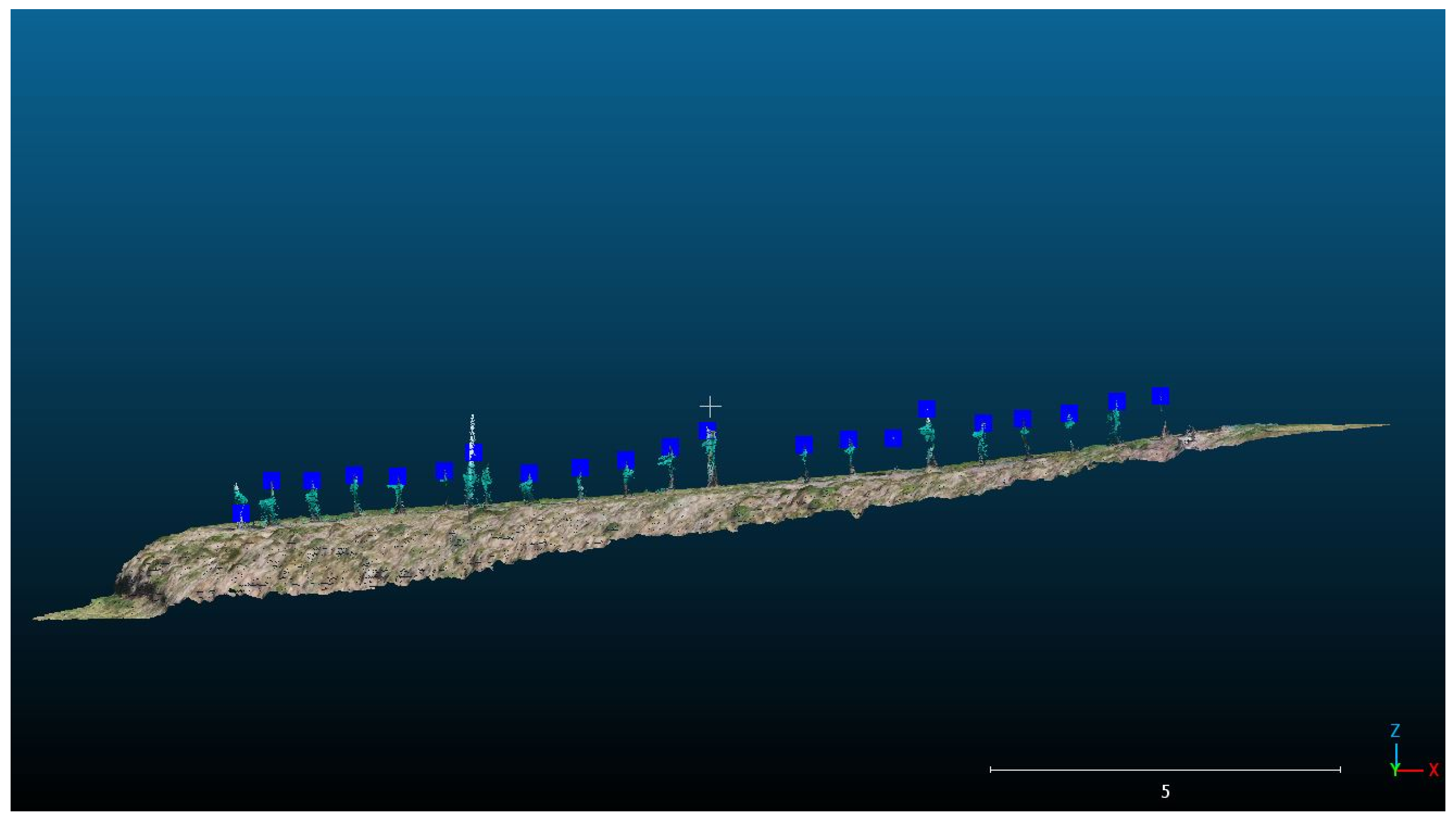
The derivation of exact vine stem locations allows for accurate mapping and monitoring of individual vines. Precise stem locations facilitate targeted interventions, such as optimized irrigation, fertilization, and pest control. The stem locations were derived using 3D point-cloud analysis with the software Cloud Compare (Paris, France) version 2.12.4. For the derivation of single plant locations, the dataset from 8 April 2023 was analyzed. At this time, the vines are in the phenological stage of budburst, where leaves are not yet developed and only the wooden part of the plants is present [30]. As in the study of Ruess et al. [37], a planar mesh surface was fitted to the 3D point cloud to serve as the base surface for further analysis. The distance between the point cloud and the generated mesh surface was then calculated, with the maximum distance values corresponding to the tops of the vine stems. For each vine stem, the scalar field contained all X, Y, and Z coordinates of the individual points. The maximum Z-values within the grapevine trunk clusters were identified, and their corresponding X and Y coordinates were recorded. The exported coordinates representing the maximum distance between the surface and the point cloud are georeferenced using the Austrian geodetic system Lambert ETRS 1989 (Figure 3). These coordinates indicate the positions of individual vines at a height of approximately 20 cm. At this height, the vine trunks remain vertical, with no significant slope angles observed.

After deriving the locations of the individual vine stems across the entire vineyard, the results from the OBIA framework, which identified the vine row objects, were combined with the coordinates of the plants. This allowed the segmentation of the vine row polygons into individual plant polygons. The equidistant point between each pair of vine stem coordinates was calculated. In the next step, the vine row polygons were split at the location of the equidistant midpoints, resulting in individual plant polygons as shown in Figure 4. Reference points were measured using a Leica GNSS at the vine trunk’s base. A total of 21 vines were measured and compared to the automatically derived locations based on their Euclidean distance. The average distance between the detected points and the reference points is 10.7 cm.

2.4.3. Vine Performance Analysis

Several studies show that vegetative health and multispectral vegetation indices are strongly correlated. The NDRE is among other indices capable of providing information about the health status of grapevines and the variability within a vineyard. Using the single plant polygonal objects, the NDRE was calculated as a mean value averaged over the extent of the individual vine canopies.

$$NDRE={\displaystyle \frac{NIR-RedEdge}{NIR+RedEdge}}$$

(4)

After using Equation (4), vegetation index maps (Figure 5) were produced for the timestamps shown in Table 1 except for the dormant dataset [38]. The indices were calculated using the Python Plugin from ArcGIS Pro (Esri, Redlands, CA, USA) version 3.3.0. The single vine objects were used to extract the mean NDRE value within each vine polygon using zonal statistics in ArcGIS Pro. The average index values are stored within the point feature class that holds the position for the 1063 vines.

On 6 October 2023, the day of harvest and the final UAS data acquisition, 34 vines were harvested prior to the UAS flight and weighed individually. These 34 reference plants were used to establish a linear regression to assess whether the mean NDRE value per vine correlates with the actual harvest weight. The datasets are directly comparable, as the time gap between harvesting/weighing and multispectral data collection was approximately one hour. To evaluate the relationship between vine health and actual yield, a linear regression analysis was performed using RStudio (version 2025.05.1 Build 513) to model the relationship between per-vine NDRE values and corresponding harvest weights (reference vines n = 34). The regression shows a significant result (p < 0.001), with an R² value of 0.73, indicating that approximately 73% of the variability in vine yield can be explained by the NDRE value (Figure 6). The model can be described by Equation (5).

$$Harvest Weight=-1.71+8.42\times NDRE value$$

(5)

Although the coefficient for NDRE is 8.42, this should be interpreted in the context of the typical NDRE value range for healthy vegetation (approximately 0.20–0.40). A 0.1 unit increase in NDRE therefore corresponds to a ~0.84 kg increase in predicted vine yield, which aligns well with actual harvest values observed in the dataset.

The residual standard error was 0.186 kg, and the 95% confidence intervals confirmed a significant and stable relationship between NDRE and yield.

2.4.4. Spatial Patterns and Cluster Analysis of NDRE Values

The geospatial analysis of NDRE values for individual vines within the study site was conducted using ArcGIS Pro. To determine the presence of spatial autocorrelation in the distribution of NDRE values, a Global Moran’s I calculation was performed. Spatial autocorrelation was assessed for each dataset, with the results presented in

Table 3. Measures of the Global Moran’s I, calculated for all UAS-mission dates.

Timestamp	Phenological Stages	Moran’s Index	p-Value	Z-Score
23 September 2022	Harvest	0.52	0.00	35.44
14 July 2023	Flowering	0.69	0.00	46.78
16 August 2023	Veraison	0.7	0.00	47.49
6 October 2023	Harvest	0.73	0.00	48.93

. Spatial autocorrelation is assumed when the physiological parameters of a plant are influenced by those of neighboring plants, based on their geographic arrangement [39]. For the initial test of autocorrelation, Global Moran’s I was calculated, which measures the degree of relationship among neighboring values within a spatial pattern [40]. The null hypothesis (H₀) states that the mean NDRE values per vine are randomly distributed across the vineyard, while the alternative hypothesis (H₁) claims that the values exhibit spatial clustering.

The Global Moran’s I values calculated across all timestamps confirm the presence of spatial autocorrelation in the observed NDRE values. Moran’s I values close to 1 indicate clustering, suggesting that neighboring regions tend to have similar values. Statistical significance was assessed using the p-value and z-score. A small p-value indicates that the observed spatial autocorrelation is highly unlikely to result from random chance. The z-score represents the number of standard deviations by which the observed Moran’s I deviates from the expected value under the null hypothesis (H₀), which assumes no spatial autocorrelation [41]. Z-scores exceeding 35 across all observations demonstrate strong clustering in the NDRE values.

Now that the Global Moran’s I indicated strong spatial autocorrelation for the NDRE values of the single vines, there was interest in identifying local patterns. The Local Indicators of Spatial Association (LISA) were calculated for the index values to detect hotspots, cold spots, and outliers at a single plant level. The method identifies areas where high NDRE values are among other high values, and it detects outliers and low-value zones.

Local spatial autocorrelation of per-vine NDRE values was calculated using the LISA framework in ArcGIS Pro (ESRI, Redlands, CA, USA) version 3.3.0. Spatial relationships were defined using an inverse distance method with a threshold distance of 3.0 m, corresponding to the typical planting layout of the vineyard, with 1 m vine spacing and approximately 2 m between rows. This configuration ensures that each vine is analyzed in the context of its immediate surroundings while gradually reducing the influence of more distant neighbors within the threshold. Inverse distance weighting is particularly suitable in this context as it reflects the assumption that neighboring vines closer in proximity have stronger spatial relationships in terms of vigour and resource conditions. Spatial weights were row-standardized to normalize the total influence of each vine’s neighborhood, making the analysis robust to variations in neighbor count, especially at plot edges or in irregular planting zones. Statistical significance was determined using 999 random permutations at α = 0.05. This configuration enabled the detection of localized clusters and spatial outliers in vine vigour, supporting fine-scale analysis of spatial patterns within the vineyard [42]. After this, clusters were built for all four timestamps across all 1063 vines based on their NDRE values. The clusters are separated as follows:

• High performing vines (HP): areas with high NDRE values with neighbors of high values
• High–low outliers (HL): vines with high NDRE values with neighbors of low values (outlier)
• Low–high outliers (LH): vines with low NDRE values with neighbors of high values (outlier)
• Low performing vines (LP): areas with low NDRE values with neighbors of low values
• Not significant (NS): areas where NDRE values are randomly distributed

Clusters were classified as follows: High Performing (HP) if both the NDRE value and its spatially lagged value are above the global mean NDRE. Vines were classified as Low Performing (LP) if both their NDRE value and the average NDRE of their surrounding neighbors (lagged value) were below the global mean. Vines were considered high–low outliers (HL) when their NDRE value was above the global mean, but their neighbors’ average was below. Conversely, low–high outliers (LH) had NDRE values below the global mean, while their surrounding neighbors were above it [41,43].

3. Results of Vineyard Dynamics Analysis

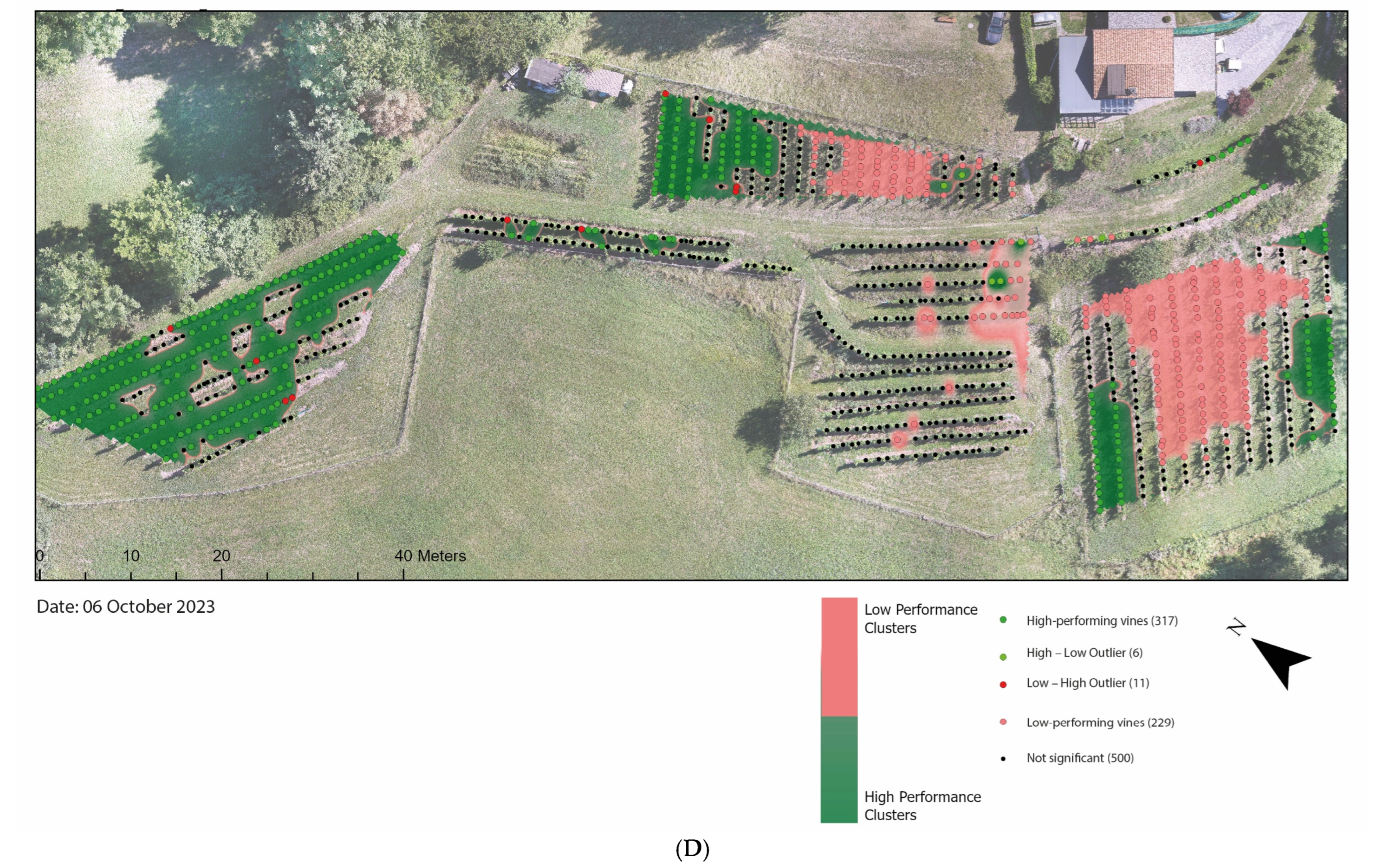
At this point, the analysis results provide insights into vineyard dynamics over the four observation dates shown in Table 1. This observation prompted a closer investigation to identify where clusters shift over time and how the vineyard changes from the end of the 2022 growing season to the end of 2023. This helps vineyard managers identify zones of persistent stress, outliers that could possibly form low performance clusters and areas, where the vine conditions are stable at the specific acquisition dates. Figure 7 illustrates the clustering results based on Local Indicators of Spatial Association, calculated from individual NDRE values. The map visualizes the spatial distribution of vine performance clusters, revealing patterns of vine health across the vineyard. Each cluster type offers specific insights into the spatial dynamics of vegetation vigour. The information is critical for precision viticulture, supporting targeted interventions such as localized irrigation, fertilization, or pest control. The identification of outlier vines (HL and LH) further enables investigation into site-specific factors that may be affecting vine performance. Additionally, tracking changes in these clusters over time provides valuable information about vine health dynamics and the effectiveness of vineyard management strategies throughout the growing season.

The end of the 2022 growing season marks a dominance of NS clusters, where the vine’s NDRE values lack significant spatial patterns for 745 vines. Throughout the next growing season, the number of NS clustered vines decreases. This suggests an increase in spatially structured patterns as the 2023 growing season progresses. A growth in HP clusters can be investigated from 107 vines at the end of the 2022 season to 317 vines at the end of 2023, indicating improved vegetation health and stronger clustering of high NDRE values closer to the harvest date. The low-performing clustered vines remain relatively stable ranging from 176 vines to 229 vines across the four observation dates. The outliers represent areas where individual vines deviate from their neighboring plants, suggesting localized anomalies, starting points of emerging problems, or edge effects. By utilizing localized information, vineyard managers can use maps or exact coordinates of specific plants to carry out precise interventions such as pruning, irrigation, or fertilization.

Figure 8 shows the distribution of single vine NDRE values across spatial clusters over four timestamps. At the end of the 2022 season, the HP cluster contains relatively few vines, with NDRE values between 0.3 and 0.4. In contrast, by 2023, the HP cluster comprises 279 vines with NDRE values exceeding 0.6, indicating a general increase in canopy vigour. In August 2023, a marked decrease in HP vines is evident, with their NDRE values ranging from 0.3 to 0.6, while LP vines exhibit generally lower NDRE values. By the final timestamp at harvest (October 2023), a sharp increase in NDRE values can be observed, with HP vines now ranging from 0.5 to approximately 0.8.

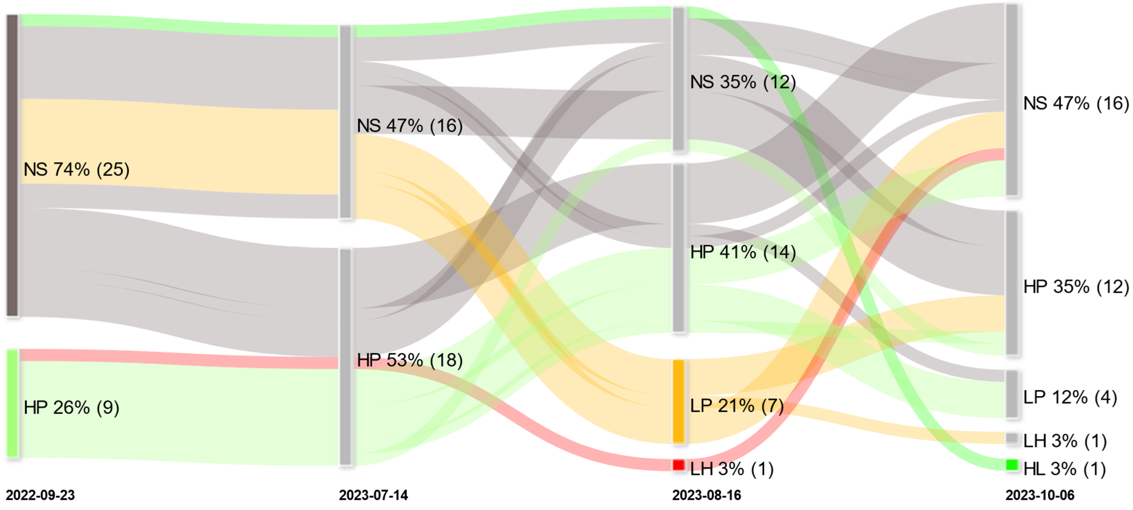
The harvest weight was derived from 34 reference plants across the vineyard on the day of the last data acquisition mission (6 October 2023). The berry weights were used to validate if the mean NDRE index per vine correlates with yield and to assess if NDRE can reliably reflect actual vine productivity. The correlation coefficient (0.73) is indicating a strong positive relationship between NDRE and harvest weight. For the 34 reference vines, a Sankey chart (Figure 9) was created to dynamically show how the vines behave over time and through which cluster group they are moving. At the end of the 2022 season, nine of the thirty-four reference vines were clustered as high-performing (HP) plants. The first date of the 2023 season in the phenology phase flowering shows that all nine vines plus nine other vines are now in this cluster. In the following month, fourteen of those HP vines remain in the same cluster, and one becomes a low–high outlier (LH) which is a plant with low NDRE value among high performers. Three vines move to the NS cluster where values are randomly dispersed. The 14 remaining vines then move to the low-performing (LP) cluster and to the NS cluster.

To see if the vigour clusters derived from UAS-based NDRE mapping reflect the actual vine productivity, the harvest weights of the 34 reference vines were analyzed in relation to their final vigour cluster assignments.

Figure 10 illustrates the distribution of harvest weights among the 34 reference vines according to their final spatial cluster status in October 2023. Vines classified as high performing (HP) exhibit the highest average yield at 1.93 kg, with the overall maximum harvest weight of 2.5 kg also observed within this group. The HP cluster shows the broadest yield range (1.45–2.5 kg), indicating strong productivity potential coupled with variability. In contrast, vines in the low-performing (LP) cluster display consistently lower yields, with a maximum of 1.8 kg. Vines categorized as non-significant (NS) exhibit a wide spread of harvest weights (1.2–2.02 kg), suggesting that spatial clustering did not consistently predict their productivity. These findings support the relevance of LISA-based vigour clusters for identifying yield performance patterns, particularly for distinguishing high- and low-yielding vines at harvest.

4. Discussion

The presented study shows the technical feasibility to monitor a vineyard at the single vine scale across time using UAS-based data acquisition techniques, photogrammetric image processing, OBIA, and 3D point-cloud analysis to generate datasets that can be used for spatiotemporal clustering methods to show vine performance variations within a vineyard. A UAS equipped with a high-resolution multispectral sensor providing 10 band spectral resolution and a very high resolution RGB sensor with 45 megapixels of spatial resolution, that can be triggered simultaneously, made it possible to cover the whole study site with one single flight. This method is time efficient and ensures the same lighting conditions for the multispectral survey as well as for the RGB data collection. This makes the datasets comparable and ready for processing. The data processing was a straight-forward process that led to the creation of georeferenced outputs like orthomosaics, surface models, and 3D point-clouds that represent the vegetative period of 2023.

The 3D point cloud from a dataset collected on 8 April 2023 was used to detect single vine trees. At the time of data collection, the plants did not develop foliage yet, making it possible to detect the stems in the 3D point cloud. Recent studies used deep learning models to detect vine trees under certain lighting conditions and achieved sufficient results [3]. However, those methods require training data and are dependent on weather conditions. In contrast, the presented method is independent from lighting and derives the transformed coordinates of single vine plants with a mean Euclidean distance to reference measurement of 10.7 cm.

After single vine detection, canopy segmentation was performed. Pixel-based methods often apply thresholds to color or reflectance values [44], and include unsupervised clustering that allocates clusters based on pixel value similarity rather than topology [6,44]. In contrast, OBIA is well-suited for high-resolution data and handles pixel heterogeneity better than pixel-based methods [45]. An OBIA framework was implemented to classify the scene and distinguish vines from other objects and to derive vine row objects. Existing studies show frameworks for vine segmentation where the algorithms are dependent on just height based data and pre-clipping of the scene to exclude other vegetation types that may occur in the scene [17]. This study shows a framework where the whole scene is processed and vine objects are classified based on geometric and spectral characteristics. The vine objects were joined with the vine location point features, and splits were created at the midpoint between each pair of adjacent vines to assign canopy segments to individual plants based on the assumption that vines grow irregularly into each other and can be separated by using a systematic approach where the equidistant mid-points are considered.

The NDRE data of four observation dates were used together with single vine objects to calculate the average VI value per vine canopy. Local Indicators of Spatial Association (LISA) was chosen for clustering as it accounts for both the magnitude of NDRE values and their spatial arrangement [46]. This spatially explicit method allows for the detection of not only homogeneous zones of vine vigour but also local outliers, offering a more nuanced understanding of spatial patterns than non-spatial clustering approaches. Applied across three phenological stages, LISA enables the temporal tracking of vine performance while preserving spatial context essential for targeted vineyard management. The shifts in cluster compositions highlights changes in vine health based on the single vine’s average NDRE values and unveils spatial patterns.

Figure 8 shows the distribution of NDRE values across spatial clusters. Vines within the low-performing (LP) cluster show NDRE values of up to 0.3, suggesting that some vines with moderate NDRE values are still classified as low-performing due to their spatial context. This highlights a key advantage of the spatial clustering approach as it does not evaluate vine vigour in isolation but considers the spatial autocorrelation of NDRE values. In doing so, it identifies contiguous zones of stress or high performance that may not be apparent from raw isolated NDRE values alone. Since many vineyard stressors such as disease, water scarcity, or nutrient deficiency propagate spatially, analyzing clustered patterns provides more actionable insight for vineyard managers than purely point-based assessments [47]. In August 2023, the number of HP vines decreased noticeably, with NDRE values between 0.3 and 0.6, while LP vines showed generally lower NDRE values. By harvest in October 2023, NDRE values for HP vines increased to a range of 0.5 to about 0.8.

Some LP-clustered vines at this stage still reach NDRE values as high as 0.5, which is typically considered high vigour. However, their LP classification reflects the spatial context. Despite their own strong NDRE values, these vines are embedded in neighborhoods where surrounding vines display comparatively lower NDRE levels. LISA-based clustering interprets such local contrasts and assigns cluster status accordingly. This capacity to reveal spatial outliers and edge cases makes the method particularly valuable for detecting subtle or emerging stress zones that might otherwise be overlooked in non-spatial analyses. The individual NDRE values of vines clustered as NS where NDRE values are randomly distributed range from 0.2 to 0.4 except in the last observation date where the randomly distributed NDRE values are present in the upper part of the vigour value range. As overall vine vigour increased toward harvest, more vines displayed high NDRE values, but not all formed coherent spatial clusters and were then clustered as NS.

The ability to backtrack individual vines using the Sankey diagram (Figure 9) offers valuable insights into the temporal dynamics of vine performance. For the 34 reference vines, this retrospective tracking allows the identification of performance trajectories, highlighting vines that consistently remained in the high-performing (HP) cluster, as well as those that declined or fluctuated throughout the season. This can help vineyard managers understand which vines responded well to environmental conditions or interventions and which showed early signs of stress, potentially informing future management decisions, targeted monitoring, and resource allocation.

A noticeable decline in the overall number of vines classified as high performing (HP) was observed between July, 2023, and August 2023. During the flowering stage, 279 vines were assigned to the HP cluster, whereas by the veraison stage in August 2023, this number dropped significantly to 188. This period is referred to as Phase 1. Phase 2 spans from August 2023, to October 2023, covering the phenological stages from veraison to harvest. During this period, the number of HP vines increased again, reaching 317 by harvest.

Low-performing (LP) vines showed signs of persistent stress and remained relatively stable across the phenological stages, fluctuating between 227 and 229 vines. The outliers, which are critical for early stress detection, also showed limited variation—rising to twenty-five vines in veraison and dropping to six by harvest.

To explore the sharp decline and subsequent recovery in HP vines, weather data from the vineyard location were retrieved from meteoblue History+ (meteoblue AG, Basel, Switzerland). As shown in

Table 4. Weather metrics (mean and cumulative) for the exploratory analysis of NDRE decline across phenological stages.

Phase	1	2
HP	−91	+129
LP	−2	+4
NS	−78	+117
HL	+16	−19
LH	−1	+3
Mean temp max (°C)	24.98	24.32
Mean of max temp (°C)	24.47	20.27
Cum. ET0 (mm)	201.88	121.33
Cum. Rain (mm)	215.00	400.20
Days > 30 °C	6.00	0.00
Cum. Sun (h)	535.06	397.28
Soil temp (10 cm) mean (°C)	14.53	12.86

, Phase 1 was characterized by a higher mean maximum temperature compared to Phase 2. Additionally, there were 6 days above 30 °C, which may have stressed the vines. A heatwave, as defined by at least five consecutive days with maximum temperatures exceeding the average of daily maximum temperatures by 5 °C, was observed during this period [48].

Phase 1 also recorded relatively low precipitation and high evapotranspiration rates, along with higher soil temperatures and longer sun duration than Phase 2. In contrast, Phase 2 saw a significant increase in the number of HP vines, accompanied by more favorable weather conditions—no heatwave events, twice the rainfall amount compared to Phase 1, and lower evapotranspiration. Reduced soil temperatures and less solar radiation likely contributed to the recovery observed by harvest.

This comparison with weather data is exploratory and serves as a foundation for future investigations. In upcoming growing seasons, a denser data portfolio combining UAS and satellite imagery will be used to strengthen and expand the analysis. With more observation dates available, vine conditions can be correlated more robustly with environmental factors. The proposed method is applicable to other crops, but limitations could arise in crops where plant spacing is very dense making it difficult to locate individual plants. The transferability to other crops will be investigated in future research projects.

Further research will also consider the fact that vines exhibit different spectral and geometric characteristics depending on their phenological stage. A temporarily lower spectral signal does not necessarily indicate poor health. Therefore, future approaches will employ machine learning methods capable of comparing entire spectral signal curves against reference patterns to incorporate physiologically normal vine behavior into classification and assessment workflows.

5. Conclusions

This feasibility study demonstrates how the position of individual vines can be identified without the need for training data and independently of lighting and weather conditions. Using these georeferenced vine locations and an object-based image analysis (OBIA) framework that does not require prior clipping or masking of the study area, vine rows and single-plant canopy masks were successfully segmented. These masks enabled the calculation of mean NDRE values across the full canopy of each vine at four time points, covering three phenological stages. Using Local Indicators of Spatial Association (LISA), these spectral values were analyzed to detect spatial autocorrelation, allowing the identification of neighborhood relationships between vines.

The clustering revealed groups of vines in spatial proximity that exhibited high NDRE values and formed high-performing (HP) clusters. Zones of persistent stress were also delineated, indicating areas that may require intervention. LISA enabled the detection of spatial outliers—vines with low NDRE values surrounded by high-performing neighbors—which could signal the early formation of stress zones. Since all vines were georeferenced, they can be accurately located in the field using DGNSS, allowing for targeted interventions.

The proposed framework provides a robust, data-driven approach for monitoring vine health at the individual plant level throughout the growing season. The methods enable spatial and temporal analysis of vine vigour, supporting precise, site-specific viticulture decisions. By enabling the timely detection of stress zones and supporting site-specific management, this approach could enhance both yield optimization and resource efficiency in precision viticulture.

References

1. Arnó, J.; Martínez Casasnovas, J.A.; Ribes Dasi, M.; Rosell, J.R. Review. Precision viticulture. Research topics, challenges and opportunities in site-specific vineyard management. Span. J. Agric. Res. 2009, 7, 779–790. [Google Scholar] [CrossRef]
2. Sassu, A.; Gambella, F.; Ghiani, L.; Mercenaro, L.; Caria, M.; Pazzona, A.L. Advances in Unmanned Aerial System Remote Sensing for Precision Viticulture. Sensors 2021, 21, 956. [Google Scholar] [CrossRef]
3. Gavrilović, M.; Jovanović, D.; Božović, P.; Benka, P.; Govedarica, M. Vineyard Zoning and Vine Detection Using Machine Learning in Unmanned Aerial Vehicle Imagery. Remote Sens. 2024, 16, 584. [Google Scholar] [CrossRef]
4. Aquino, A.; Millan, B.; Diago, M.-P.; Tardaguila, J. Automated early yield prediction in vineyards from on-the-go image acquisition. Comput. Electron. Agric. 2018, 144, 26–36. [Google Scholar] [CrossRef]
5. Moraye, K.; Pavate, A.; Nikam, S.; Thakkar, S. Crop Yield Prediction Using Random Forest Algorithm for Major Cities in Maharashtra State. Int. J. Innov. Res. Comput. Sci. Technol. 2021, 9, 40–44. [Google Scholar] [CrossRef]
6. Cinat, P.; Di Gennaro, S.F.; Berton, A.; Matese, A. Comparison of Unsupervised Algorithms for Vineyard Canopy Segmentation from UAV Multispectral Images. Remote Sens. 2019, 11, 1023. [Google Scholar] [CrossRef]
7. Barros, T.; Conde, P.; Gonçalves, G.; Premebida, C.; Monteiro, M.; Ferreira, C.S.S.; Nunes, U.J. Multispectral vineyard segmentation: A deep learning comparison study. Comput. Electron. Agric. 2022, 195, 106782. [Google Scholar] [CrossRef]
8. Ferro, M.V.; Sørensen, C.G.; Catania, P. Comparison of different computer vision methods for vineyard canopy detection using UAV multispectral images. Comput. Electron. Agric. 2024, 225, 109277. [Google Scholar] [CrossRef]
9. Cogato, A.; Meggio, F.; Collins, C.; Marinello, F. Medium-Resolution Multispectral Data from Sentinel-2 to Assess the Damage and the Recovery Time of Late Frost on Vineyards. Remote Sens. 2020, 12, 1896. [Google Scholar] [CrossRef]
10. Giovos, R.; Tassopoulos, D.; Kalivas, D.; Lougkos, N.; Priovolou, A. Remote Sensing Vegetation Indices in Viticulture: A Critical Review. Agriculture 2021, 11, 457. [Google Scholar] [CrossRef]
11. Sozzi, M.; Kayad, A.; Marinello, F.; Taylor, J.; Tisseyre, B. Comparing vineyard imagery acquired from Sentinel-2 and Unmanned Aerial Vehicle (UAV) platform. OENO One 2020, 54, 189–197. [Google Scholar] [CrossRef]
12. Agapiou, A. Vegetation Extraction Using Visible-Bands from Openly Licensed Unmanned Aerial Vehicle Imagery. Drones 2020, 4, 27. [Google Scholar] [CrossRef]
13. Lorenz, D.H.; Eichhorn, K.W.; Bleiholder, H.; Klose, R.; Meier, U.; Weber, E. Growth Stages of the Grapevine: Phenological growth stages of the grapevine (Vitis vinifera L. ssp. vinifera)—Codes and descriptions according to the extended BBCH scale. Aust. J. Grape Wine Res. 1995, 1, 100–103. [Google Scholar] [CrossRef]
14. Ferro, M.V.; Catania, P.; Miccichè, D.; Pisciotta, A.; Vallone, M.; Orlando, S. Assessment of vineyard vigour and yield spatio-temporal variability based on UAV high resolution multispectral images. Biosyst. Eng. 2023, 231, 36–56. [Google Scholar] [CrossRef]
15. Bannari, A.; Morin, D.; Bonn, F.; Huete, A.R. A review of vegetation indices. Remote Sens. Rev. 1995, 13, 95–120. [Google Scholar] [CrossRef]
16. Poblete-Echeverría, C.; Olmedo, G.; Ingram, B.; Bardeen, M. Detection and Segmentation of Vine Canopy in Ultra-High Spatial Resolution RGB Imagery Obtained from Unmanned Aerial Vehicle (UAV): A Case Study in a Commercial Vineyard. Remote Sens. 2017, 9, 268. [Google Scholar] [CrossRef]
17. De Castro, A.; Jiménez-Brenes, F.; Torres-Sánchez, J.; Peña, J.; Borra-Serrano, I.; López-Granados, F. 3-D Characterization of Vineyards Using a Novel UAV Imagery-Based OBIA Procedure for Precision Viticulture Applications. Remote Sens. 2018, 10, 584. [Google Scholar] [CrossRef]
18. Modica, G.; De Luca, G.; Messina, G.; Praticò, S. Comparison and assessment of different object-based classifications using machine learning algorithms and UAVs multispectral imagery: A case study in a citrus orchard and an onion crop. Eur. J. Remote Sens. 2021, 54, 431–460. [Google Scholar] [CrossRef]
19. Kerkech, M.; Hafiane, A.; Canals, R. Vine disease detection in UAV multispectral images using optimized image registration and deep learning segmentation approach. Comput. Electron. Agric. 2020, 174, 105446. [Google Scholar] [CrossRef]
20. Jurado, J.M.; Pádua, L.; Feito, F.R.; Sousa, J.J. Automatic Grapevine Trunk Detection on UAV-Based Point Cloud. Remote Sens. 2020, 12, 3043. [Google Scholar] [CrossRef]
21. Di Gennaro, S.F.; Matese, A. Evaluation of novel precision viticulture tool for canopy biomass estimation and missing plant detection based on 2.5D and 3D approaches using RGB images acquired by UAV platform. Plant Methods 2020, 16, 91. [Google Scholar] [CrossRef]
22. Haghverdi, A.; Leib, B.G.; Washington-Allen, R.A.; Ayers, P.D.; Buschermohle, M.J. Perspectives on delineating management zones for variable rate irrigation. Comput. Electron. Agric. 2015, 117, 154–167. [Google Scholar] [CrossRef]
23. Lajili, A.; Cambouris, A.N.; Chokmani, K.; Duchemin, M.; Perron, I.; Zebarth, B.J.; Biswas, A.; Adamchuk, V.I. Analysis of Four Delineation Methods to Identify Potential Management Zones in a Commercial Potato Field in Eastern Canada. Agronomy 2021, 11, 432. [Google Scholar] [CrossRef]
24. Pádua, L.; Marques, P.; Hruška, J.; Adão, T.; Peres, E.; Morais, R.; Sousa, J.J. Multi-Temporal Vineyard Monitoring through UAV-Based RGB Imagery. Remote Sens. 2018, 10, 1907. [Google Scholar] [CrossRef]
25. Matese, A.; Di Gennaro, S.F.; Berton, A. Assessment of a canopy height model (CHM) in a vineyard using UAV-based multispectral imaging. Int. J. Remote Sens. 2016, 38, 2150–2160. [Google Scholar] [CrossRef]
26. Matese, A.; Di Gennaro, S.F.; Santesteban, L.G. Methods to compare the spatial variability of UAV-based spectral and geometric information with ground autocorrelated data. A case of study for precision viticulture. Comput. Electron. Agric. 2019, 162, 931–940. [Google Scholar] [CrossRef]
27. Campos, J.; Garcia-Ruiz, F.; Gil, E. Assessment of Vineyard Canopy Characteristics from Vigour Maps Obtained Using UAV and Satellite Imagery. Sensors 2021, 21, 2363. [Google Scholar] [CrossRef]
28. Daniels, L.; Eeckhout, E.; Wieme, J.; Dejaegher, Y.; Audenaert, K.; Maes, W.H. Identifying the Optimal Radiometric Calibration Method for UAV-Based Multispectral Imaging. Remote Sens. 2023, 15, 2909. [Google Scholar] [CrossRef]
29. Agisoft. Agisoft Metashape User Manual: Professional Edition, Version 2.0; Agisoft LLC: Saint Petersburg, Russia, 2023. [Google Scholar]
30. Westover, F. Grapevine Phenology Revisited. Available online: https://winesvinesanalytics.com/features/article/196082/Grapevine-Phenology-Revisited (accessed on 1 July 2022).
31. Pricope, N.G.; Halls, J.N.; Mapes, K.L.; Baxley, J.B.; Wu, J.J. Quantitative Comparison of UAS-Borne LiDAR Systems for High-Resolution Forested Wetland Mapping. Sensors 2020, 20, 4453. [Google Scholar] [CrossRef]
32. Zhang, W.; Qi, J.; Wan, P.; Wang, H.; Xie, D.; Wang, X.; Yan, G. An Easy-to-Use Airborne LiDAR Data Filtering Method Based on Cloth Simulation. Remote Sens. 2016, 8, 501. [Google Scholar] [CrossRef]
33. Njambi, R. nDSMs: How digital Surface Models and Digital Terrain Models Elevate Your Insights. Available online: https://up42.com/blog/ndsms-how-digital-surface-models-and-digital-terrain-models-elevate-your (accessed on 8 August 2023).
34. Trimble, eCognition Developer User Guide; Trimble Germany GmbH: Munich, Germany, 2022.
35. Rosso, P.; Nendel, C.; Gilardi, N.; Udroiu, C.; Chlebowski, F. Processing of remote sensing information to retrieve leaf area index in barley: A comparison of methods. Precis. Agric. 2022, 23, 1449–1472. [Google Scholar] [CrossRef]
36. Clevers, J.G.P.W. Application of the WDVI in estimating LAI at the generative stage of barley. ISPRS J. Photogramm. Remote Sens. 1991, 46, 37–47. [Google Scholar] [CrossRef]
37. Ruess, S.; Paulus, G.; Lang, S. Automated Derivation of Vine Objects and Ecosystem Structures Using UAS-Based Data Acquisition, 3D Point Cloud Analysis, and OBIA. Appl. Sci. 2024, 14, 3264. [Google Scholar] [CrossRef]
38. Maccioni, A.; Agati, G.; Mazzinghi, P. New vegetation indices for remote measurement of chlorophylls based on leaf directional reflectance spectra. J. Photochem. Photobiol. 2001, 61, 52–61. [Google Scholar] [CrossRef]
39. Mathur, M. Spatial Autocorrelation analysis in plant population: An overview. J. Appl. Nat. Sci. 2015, 17, 501–513. [Google Scholar] [CrossRef]
40. Boots, B.; Getis, A. Point Pattern Analysis. In Web Book of Regional Science, RJackson, R., Ed.; West Virginia University: Morgantown, WV, USA, 1988. [Google Scholar]
41. Moraga, P. Spatial Statistics for Data Science: Theory and Practice with R. Available online: https://www.paulamoraga.com/book-spatial/spatial-autocorrelation.html (accessed on 1 January 2025).
42. Anselin, L. Local Indicators of Spatial Association—LISA. Geogr. Anal. 1995, 27, 93–115. [Google Scholar] [CrossRef]
43. Blanford, J.; Kessler, F.; Griffin, A.; O’Sullival, D. Project 4: Calculating Global Moran’s I and the Moran Scatterplot. Available online: https://www.e-education.psu.edu/geog586/node/672 (accessed on 1 January 2025).
44. Ferreira, M.P.; Féret, J.-B.; Grau, E.; Gastellu-Etchegorry, J.-P.; do Amaral, C.H.; Shimabukuro, Y.E.; de Souza Filho, C.R. Retrieving structural and chemical properties of individual tree crowns in a highly diverse tropical forest with 3D radiative transfer modeling and imaging spectroscopy. Remote Sens. Environ. 2018, 211, 276–291. [Google Scholar] [CrossRef]
45. Blaschke, T. Object based image analysis for remote sensing. ISPRS J. Photogramm. Remote Sens. 2010, 65, 2–16. [Google Scholar] [CrossRef]
46. Catania, P.; Ferro, M.V.; Orlando, S.; Vallone, M. Grapevine and cover crop spectral response to evaluate vineyard spatio-temporal variability. Sci. Hortic. 2025, 339, 113844. [Google Scholar] [CrossRef]
47. Dalton, D.T.; Hilton, R.J.; Kaiser, C.; Daane, K.M.; Sudarshana, M.R.; Vo, J.; Zalom, F.G.; Buser, J.Z.; Walton, V.M. Spatial Associations of Vines Infected With Grapevine Red Blotch Virus in Oregon Vineyards. Plant Dis. 2019, 103, 1507–1514. [Google Scholar] [CrossRef]
48. Fraga, H.; Molitor, D.; Leolini, L.; Santos, J.A. What Is the Impact of Heatwaves on European Viticulture? A Modelling Assessment. Appl. Sci. 2020, 10, 3030. [Google Scholar] [CrossRef]
Figure 1. Study site in Carinthia, Austria—a 0.7 ha vineyard on a south/west-facing slope (17.4° incline, 750 m elevation) trunks (Adapted from: “Automated derivation of vine objects and ecosystem structures, using UAS-based data acquisition, 3D point-cloud analysis and OBIA”).
Remotesensing 17 03354 g001
Figure 2. The DJI M350 RTK equipped with two sensors (multispectral and RGB) triggered at the same time.
Remotesensing 17 03354 g002
Figure 3. Maximum values from the mesh-to-cloud distance calculation, representing the tips of individual vine trunks shown as blue rectangles (adapted from “Automated derivation of vine objects and ecosystem structures, using UAS-based data acquisition, 3D point-cloud analysis and OBIA”).
Remotesensing 17 03354 g003
Figure 4. Detailed map illustrating vine objects delineated using an OBIA framework, combined with validated single-plant locations. The polygons were divided at equidistant points between each pair of vine stem coordinates.
Remotesensing 17 03354 g004
Figure 5. NDRE raster dataset of the vineyard from multispectral data captured at the phenological stages harvest, veraison, flowering.
Remotesensing 17 03354 g005
Figure 6. Relationship between NDRE (x) and harvest weight in kilograms (y) for individual vines, showing a positive correlation (R2 = 0.73). Each point represents a single vine; the multispectral data for the NDRE was acquired 1h before harvest on 6 October 2023.
Remotesensing 17 03354 g006
Figure 7. (AD). Spatial clustering of NDRE values for individual vines across four different dates. Each map displays LISA classification of vines into high-performance vines, low-performance vines, high–low outliers, low–high outliers and areas with non-significant clustering shown in black. The number of plants per category is indicated in parentheses in the legend. Accompanying histograms summarize the NDRE value distributions, providing an overview of overall vegetation status on each respective date.
Remotesensing 17 03354 g007aRemotesensing 17 03354 g007bRemotesensing 17 03354 g007c
Figure 8. Histograms of NDRE values across four time points, showing the distribution of vine vigour by LISA cluster type.
Remotesensing 17 03354 g008
Figure 9. Cluster transitions over time shown as a Sankey diagram. Each flow is color-coded at the date of its first appearance; the same color is retained in later and previous panels so that paths can be traced back to their origin. Labels indicate the cluster and its prevalence (percentage, count).
Remotesensing 17 03354 g009
Figure 10. Boxplot showing the distribution of harvest weights (kg) for 34 reference vines grouped by final vigour cluster: high-performance vines (HP), low-performance vines (LP), and not significant (NS).
Remotesensing 17 03354 g010