Article

Satellite-Based Multi-Decadal Shoreline Change Detection by Integrating Deep Learning with DSAS: Eastern and Southern Coastal Regions of Peninsular Malaysia

by
Saima Khurram
1,
Amin Beiranvand Pour
1,*,
Milad Bagheri
1,2,
Effi Helmy Ariffin
1,
Mohd Fadzil Akhir
1 and
Saiful Bahri Hamzah
3
1
Institute of Oceanography and Environment (INOS), Higher Institution Center of Excellence (HICoE) in Marine Science, Universiti Malaysia Terengganu (UMT), Kuala Nerus 21030, Terengganu, Malaysia
2
School of Distance Education, Universiti Sains Malaysia, Gelugor 11800, Pulau Pinang, Malaysia
3
Marine Technology Departement, National Water Research Institute of Malaysia (NAHRIM), Seri Kembangan 43300, Selangor, Malaysia
*
Author to whom correspondence should be addressed.
Remote Sens. 2025, 17(19), 3334; https://doi.org/10.3390/rs17193334
Submission received: 15 June 2025 / Revised: 4 September 2025 / Accepted: 24 September 2025 / Published: 29 September 2025

Abstract

Highlights

What are the main findings?
  • Deep learning (U-Net, DeepLabV3+) integrated with DSAS enables accurate, large-scale shoreline change quantification, with U-Net outperforming in precision and generalizability.
  • There is severe erosion in Kelantan (−64.9 m/yr), localized erosion in Pahang (>−50 m/yr), moderated change in Terengganu, and major accretion in Johor (>+1900 m).
What is the implication of main findings?
  • It provides a scalable framework for long-term coastal monitoring and climate adaptation.
  • It supports evidence-based coastal management and policy by pinpointing erosion hotspots and evaluating human interventions.

Abstract

Coasts are critical ecological, economic and social interfaces between terrestrial and marine systems. The current upsurge in the acquisition and availability of remote sensing datasets, such as Landsat remote sensing data series, provides new opportunities for analyzing multi-decadal coastal changes and other components of coastal risk. The emergence of machine learning-based techniques represents a new trend that can support large-scale coastal monitoring and modeling using remote sensing big data. This study presents a comprehensive multi-decadal analysis of coastal changes for the period from 1990 to 2024 using Landsat remote sensing data series along the eastern and southern coasts of Peninsular Malaysia. These coastal regions include the states of Kelantan, Terengganu, Pahang, and Johor. An innovative approach combining deep learning-based shoreline extraction with the Digital Shoreline Analysis System (DSAS) was meticulously applied to the Landsat datasets. Two semantic segmentation models, U-Net and DeepLabV3+, were evaluated for automated shoreline delineation from the Landsat imagery, with U-Net demonstrating superior boundary precision and generalizability. The DSAS framework quantified shoreline change metrics—including Net Shoreline Movement (NSM), Shoreline Change Envelope (SCE), and Linear Regression Rate (LRR)—across the states of Kelantan, Terengganu, Pahang, and Johor. The results reveal distinct spatial–temporal patterns: Kelantan exhibited the highest rates of shoreline change with erosion of −64.9 m/year and accretion of up to +47.6 m/year; Terengganu showed a moderated change partly due to recent coastal protection structures; Pahang displayed both significant erosion, particularly south of the Pahang River with rates of over −50 m/year, and accretion near river mouths; Johor’s coastline predominantly exhibited accretion, with NSM values of over +1900 m, linked to extensive land reclamation activities and natural sediment deposition, although local erosion was observed along the west coast. This research highlights emerging erosion hotspots and, in some regions, the impact of engineered coastal interventions, providing critical insights for sustainable coastal zone management in Malaysia’s monsoon-influenced tropical coastal environment. The integrated deep learning and DSAS approach applied to Landsat remote sensing data series provides a scalable and reproducible framework for long-term coastal monitoring and climate adaptation planning around the world.

1. Introduction

Coastlines serve as critical ecological, economic, and social interfaces between terrestrial and marine systems. They are home to vital ecosystems, support fisheries and tourism industries, and accommodate significant portions of the global population [1,2]. Approximately 40% of the world’s population lives within 100 km of the seashore, and the increasing demand for land resources has led to extensive reclamation activities (e.g., aquaculture and port terminals) [3]. Consequently, these dynamic environments are under increasing stress from both natural processes and anthropogenic activities [4,5,6,7,8,9,10]. Coastal erosion, rising sea levels, and sedimentation changes, exacerbated by climate change and rapid urbanization, have heightened the need for accurate and timely shoreline monitoring [11,12,13,14]. Border detection between land and water bodies is the basis for analyzing shoreline position changes, and its delineation is crucial due to the economic and ecological significance of coastal regions [15,16]. The accuracy of shoreline extraction directly affects coastal zone planning, engineering construction, disaster prevention and mitigation, etc. Thus, accurate shoreline extraction and precise monitoring are critical for understanding erosion, accretion, and anthropogenic impacts, which are crucial for the scientific management and protection of coastal zones. Traditionally, shoreline mapping relied on field surveys, aerial photography, and manual digitization from satellite imagery [17]. While these methods offered valuable insights, they are often time-consuming, costly, and limited in spatial or temporal coverage [18,19].
Satellite remote sensing provides a systematic, synoptic framework for expanding scientific knowledge of geophysical phenomena that often lead directly or through interacting processes to natural hazards. It is crucial for coastal engineering applications to monitor shoreline changes and other components of coastal risk [18,20,21]. The development of remote sensing imagery (especially Landsat series) and geospatial technologies has since transformed shoreline monitoring by enabling consistent, repeatable, and broad-scale observations [22,23,24]. Traditional methods for shoreline extraction can be generally classified into three categories: threshold segmentation-based, classification-based, and edge detection-based methods. In practical applications, due to the challenges of selecting thresholds in complex images, these methods often struggle with complex terrains, tidal variations, and mixed land–water interfaces [25,26]. At the same time, due to the large amount, diverse types, and rich bands of currently available remote sensing image data, traditional shoreline extraction algorithms are difficult to process and analyze big remote sensing data quickly and accurately, hindering the development of practical applications [27].
To overcome these limitations, the integration of artificial intelligence (AI), particularly deep learning-based semantic segmentation models, has gained attention in recent years. Unlike conventional classification or index-based methods, deep learning algorithms can learn hierarchical spatial features from imagery, allowing for more accurate delineation of coastal boundaries [27,28]. With the emergence of deep learning, numerous architectures have been explored to enhance the precision and automation of shoreline extraction from remotely sensed data [19,23,29,30]. Zhao et al. (2022) [23] reviewed various methodologies and emphasized that the transition from conventional pixel-based classification and edge detection methods to deep convolutional neural networks (CNNs) has resulted in more reliable shoreline delineation. Despite the advent of many modern neural network architectures, both U-Net and DeepLabV3+ have remained popular choices for shoreline extraction across several shoreline extraction case studies. They often perform comparably to or even surpass more sophisticated techniques. For example, DeepSA-Net [27], an improved form of DeepLabV3+ that utilizes strip pooling and coordinate attention for capturing spatial dependencies more effectively. While these modifications did improve the segmentation accuracy marginally, the original DeepLabV3+ still performed competitively, and in some of the coastal scenarios, comparable to them. Similarly, the BDCN-UNet hybrid model developed by Mahmoud et al. (2025) [31] was designed to enhance boundary accuracy in sea–land segmentation tasks. This architecture featured advanced edge detection from the BDCN framework. Still, the author reported that when they used standard U-Net with that same dataset, the model delivered higher overall accuracy and IoU than the modified U-Net version. This finding proved that the fundamental U-Net architecture functions well and that design simplicity does not affect performance, particularly when training data are properly prepared and contextual features remain salient. Zhao et al. (2022) [23] and Khurram et al. (2025) [32] also demonstrated the strong worth of U-Net and DeepLabV3+ through their reviews. Both models were among the most widely used and stable in a wide variety of studies, and were cited to be easily deployable, efficient in learning the spatial hierarchies, and capable of adapting to a variety of remote sensing data such as Landsat, Sentinel, and UAV data. Wu et al. (2025) [33] confirmed DeepLabV3+’s adaptability beyond optical datasets by applying it to SAR imagery over a variety of coastal terrains in Japan and reporting great results.
Malaysia, with its extensive and diverse coastlines along the Peninsula, is consistently exposed to threats from the ocean, resulting in coastal erosion and sea-level rise. Even though anthropogenic activities mostly drive erosion, with a combination of natural forces, the impacts are exacerbated by climate change [34]. It has witnessed pronounced shoreline fluctuations over recent decades, particularly on the east and west coasts [35,36]. These changes not only threaten infrastructure and livelihoods but also challenge sustainable coastal zone management. For coastline extraction in the Malaysian Peninsula, this study chooses U-Net and DeepLabV3+ due to their consistent performance in the literature, even when compared with more recent, sophisticated models. Their proven ability to delineate land–water boundaries under varied coastal morphologies makes them ideal candidates for evaluating shoreline classification accuracy in the context of long-term change detection. In Malaysia, despite growing interest in AI-powered shoreline mapping, limited studies have systematically compared these architectures using locally relevant datasets and remote sensing products like Landsat remote sensing data series. Accordingly, this study aimed to fill that gap by applying both U-Net and DeepLabV3+ models to classify land and water classes from Landsat images along the Malaysian Peninsula coastline. Identical backbone training, datasets, label masks, and preprocessing pipelines were used to ensure a controlled comparison of the models’ effectiveness. The model that demonstrated superior performance was subsequently employed to extract historical shorelines from Landsat images spanning the period from 1990 to 2024, and shoreline change analysis was conducted using the Digital Shoreline Analysis System (DSAS) tool. The novelty of this study lies in its integration of deep learning-based segmentation and long-term shoreline trend analysis within a Southeast Asian context, contributing not only to methodological advancement but also to regional coastal management strategies. To the best of our knowledge, this was the first study to systematically compare U-Net and DeepLabV3+ for shoreline extraction in Malaysia and link the results directly to multidecadal shoreline change detection using DSAS.

2. Study Area

This study focuses on the coastal belt of Peninsular Malaysia, specifically targeting the eastern coasts of Kelantan, Terengganu, and Pahang and both the eastern and western coasts of Johor (Figure 1). This region represents a diverse and dynamic stretch of Malaysia’s shoreline, encompassing a range of geomorphological, ecological, and socio-economic environments. Sand beaches, river estuaries, and patches of mangrove forests are the main features of Peninsular Malaysia’s east coast, which includes Kelantan, Terengganu, and Pahang. These states face the South China Sea and are known for their monsoon-influenced climate, which brings intense wave action, particularly between November and March [36,37]. The extensive development and expansions of the urban areas of Kuala Terengganu and others have also led to shoreline recession, and areas such as Pantai Tok Jembal and Pantai Chendering have been experiencing over 5 m/year of erosion [38]. The region is also part of the East Coast Economic Region (ECER), a significant economic corridor focused on tourism, manufacturing, agriculture, and logistics, spread over 66,000 square kilometers and supporting a population of over 3.9 million [39]. The Johor province, on the other hand, has coastlines along the South China Sea (east) and the Strait of Malacca (west). The eastern shore experiences seasonal wave action and storm surges due to the Northeast Monsoon, while the western shore is relatively more stable owing to its protected geomorphology. However, in some of the areas along Tanjung Piai and Pulau Indah, it has been increasingly noted to have suffered from ship activities and coastal extensions of the ports, resulting in sediment disruption and mangrove destruction [36,40].
Malaysia’s coastal areas are governed by the intricate interaction of natural and human-induced forces. Natural drivers include wave action, monsoon winds, tidal flooding, and sea level rise. Strong winds and high-energy seas from the South China Sea brought by the northeast monsoon create high seasonal erosion, particularly in the exposed parts such as Terengganu and Pahang. Sediment supply and riverine processes also contribute to the process, and river mouths generally undergo dynamic modifications by scour and sediment deposition [40,41]. Climate change further expands these impacts because it raises sea levels, combined with more frequent dangerous natural events occurring. Studies indicate sea level rise will occur at a rate of 2.8 to 4.4 mm/year and show the east Johor coastline, along with Johor Pahang, may potentially increase by 0.71 m by 2100, according to RCP 8.5 projections [36,42]. To safeguard the coastline, Malaysia uses different coastal protection strategies. The protection strategies include revetments and groynes, breakwaters, as well as beach nourishment programs and mangrove rehabilitation efforts. In Pahang and Johor, mangrove replanting initiatives have been implemented as part of ecological restoration operations, while breakwaters and geotextile tubes have been installed to stabilize eroding shorelines [13,36]. The selected study area thus represents a mix of geomorphic conditions, socio-economic dependencies, and historical shoreline changes that make it ideal for evaluating the performance of deep learning-based shoreline extraction techniques and their application in long-term change detection and coastal management.

3. Materials and Methods

3.1. Data Acquisition

Landsat data serve as a primary tool for coastal zone research and management because they provide extended time series data, having medium spatial–temporal resolution with global coverage [43,44]. This study employed a series of Landsat data that included Landsat 4–5 Thematic Mapper (TM), Landsat 7 Enhanced Thematic Mapper Plus (ETM+), and Landsat 8 Operational Land Imager (OLI) throughout the years 1990–2024. To analyze shoreline changes along the selected coastal zones of Peninsular Malaysia, the selected years for this analysis were 1990, 1993, 1998, 2002, 2008, 2014, 2018, and 2024 (Table 1). These selected years offered comprehensive temporal observations spanning over three decades while maintaining the availability of cloud-free data across the study area.
Acquiring a single completely cloud-free Landsat image for this extensive study area was found challenging because of the presence of persistent cloud coverage over coastal and shoreline zones. The Google Earth Engine (GEE) platform helped create a single composite image from available cloud-free pixel data for each target year. A multi-image composite method in GEE, which uses cloud-free pixels from yearly monitoring, is utilized to create optimal spatial and spectral representations of shorelines.
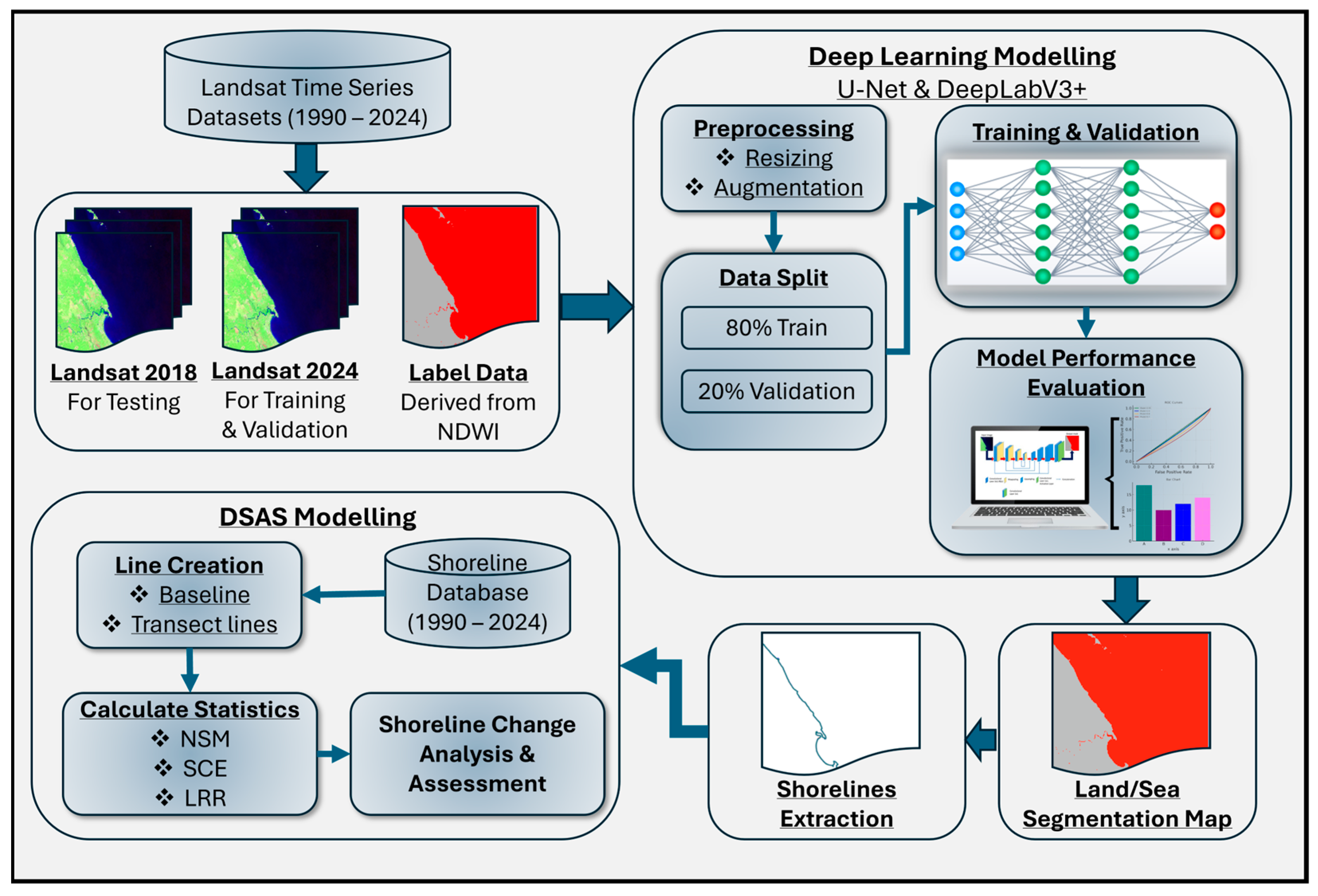
Each Landsat scene contains six critical spectral bands, which include visible, near-infrared, and short-wave infrared wavelengths because these bands effectively distinguish land–water borders and shoreline features. The Level 2 surface reflectance data is utilized, which is pre-processed with atmospheric correction to minimize radiometric inconsistencies across the time series. Deep learning models (U-Net and DeepLabV3+) underwent training and development using the 2024 composite image before applying them to the 2018 image as the main testing data. After model evaluation, the best-performing model proceeded to extract shorelines across all selected years for conducting detailed shoreline change analysis. The overall methodology framework is shown in Figure 2.

3.2. Deep Learning Models for Shoreline Extraction

The physical separation between land and water constitutes the shoreline’s most suitable definition per Dolan et al. (1991) and Moore (2000) [45,46]. This study used two semantic segmentation models, U-Net and DeepLabV3+ with ResNet-34 backbones, to extract land–water boundaries in Landsat imagery. These models were chosen due to their ability to adapt to various shoreline morphologies and their excellent performance in recent comparative investigations [30]. Supervised training employed labeled land and water image chips from the 2024 Landsat image to develop predictive models. The process of data preparation involved tiling the imagery into smaller patches, aligning them with annotated masks, and normalizing pixel values.

3.2.1. U-Net Model

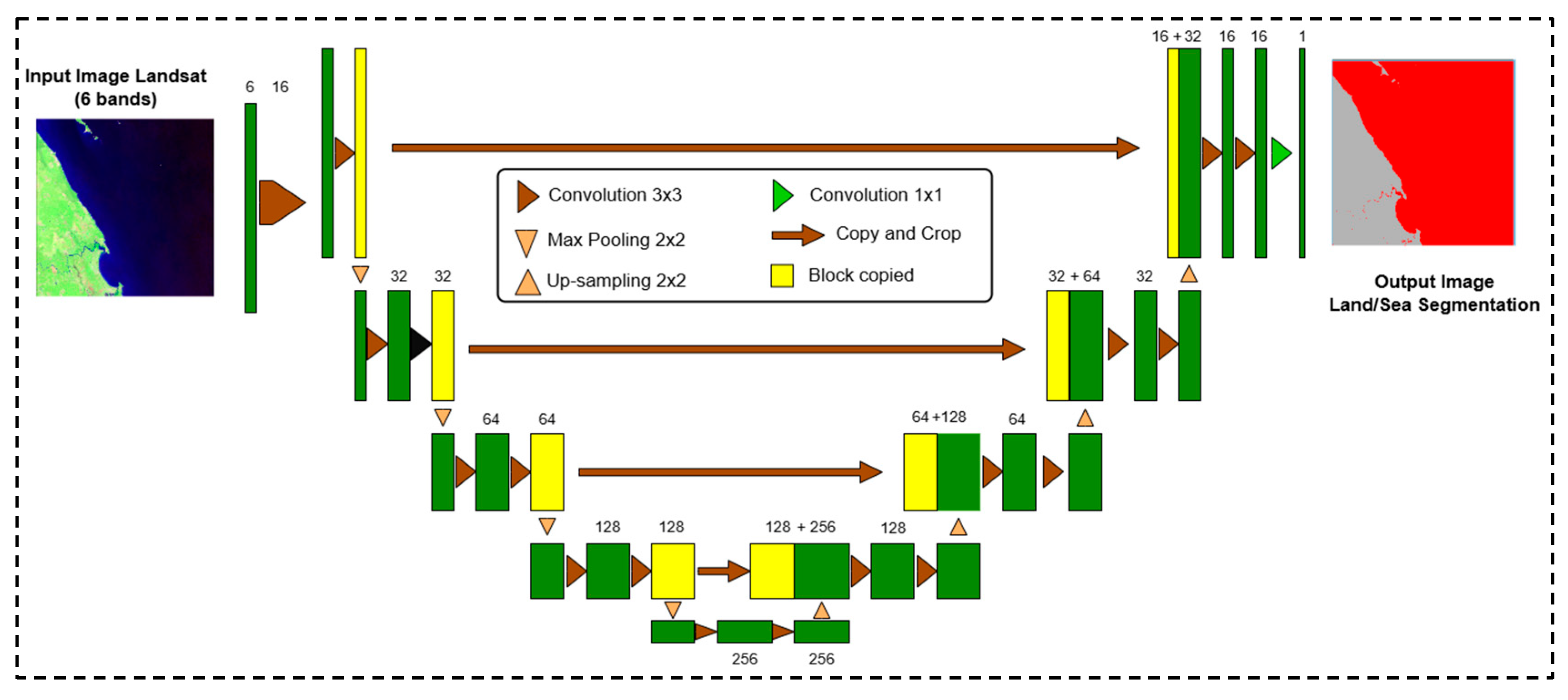
U-Net, initially developed for biomedical image segmentation, has become successful in various remote sensing applications due to its efficient integration of fine-grained details with contextual information [47,48]. The architecture combines encoder–decoder components with skip connections, which route corresponding layers from the encoder segment to the decoder segment as depicted in Figure 3 [49,50]. The input image passes through the encoder path through various convolutional layers, which use ReLU activations followed by max-pooling operations while performing progressive down-sampling. This process extracts hierarchical features and reduces the spatial dimensions of the feature maps. The decoder path restores the original input size by employing transposed convolution layers for up-sampling the feature maps. Feature maps from the encoder and decoder paths connect through skip connections to bring back detailed information and spatial characteristics that were removed by down-sampling operations.
This study adopted a U-Net model featuring ResNet34 as its backbone. ResNet34, a variant of the ResNet family, incorporates residual connections into its network structure, which protects against gradient vanishing and promotes better feature extraction. The U-Net architecture with ResNet34 backbone contains multiple repetitions of two 3 × 3 convolution layers, which end with batch normalization and ReLU activation function per layer [30]. The process of down-sampling relies on max pooling, while up-sampling happens through transposed convolution operations that result in reduced feature channel numbers.

3.2.2. DeepLabV3+ Model

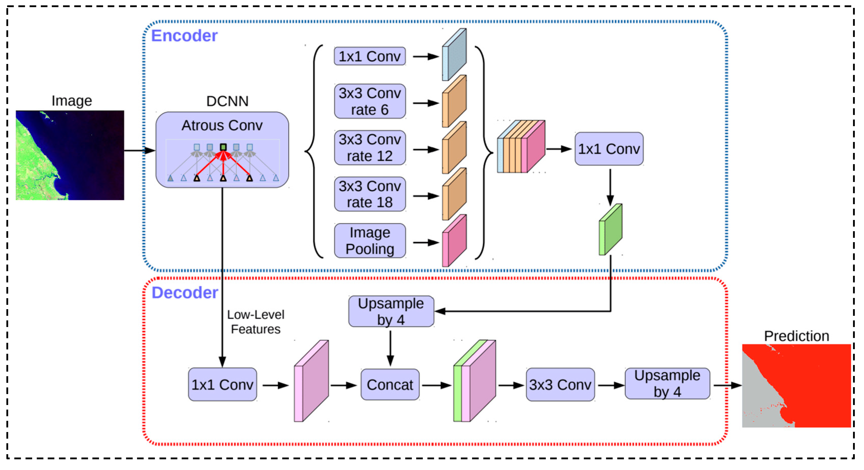
Unlike the first model, DeepLabV3+ is a more advanced segmentation model that uses atrous spatial pyramid pooling (ASPP) for multiscale contextual feature extraction while maintaining parameter efficiency [51]. The architecture was developed to resolve the problem of segmenting objects at different scales and under different spatial contexts [33]. The architecture is shown in Figure 4. The main body encoder part is a deep convolutional neural network (DCNN) with atrous convolution; a commonly used DCNN, such as ResNet, can be used, followed by the ASPP for introducing multi-scale information [52]. To capture features at different scales while retaining spatial resolution, the encoder makes use of atrous convolutions with varying values of dilation rate. Specifically, the ASPP module combines multi-scale information using several parallel atrous convolutional layers with different rates of dilation, 1 × 1 convolution, and global average pooling. The decoder path further refines the segmentation results by combining the encoded output of the input features using the low-level features of the earlier layers. The low-level features will be down-sampled through a 1 × 1 convolution and then concatenated with the up-sampled ASPP output. The concatenated features are further refined using convolutional layers and up-sampled to produce the final segmentation mask.
Both U-Net and DeepLabV3+ were implemented and trained using TensorFlow 2.8 and Keras libraries within a Jupyter Notebook environment. The models were optimized with appropriate loss functions (e.g., binary cross-entropy, dice loss) and training strategies (e.g., data augmentation, early stopping). Hyperparameters, such as learning rate, batch size, and number of epochs, were tuned to achieve optimal performance for the specific task of shoreline extraction in the study area.

3.2.3. Training and Inference Procedure

Both deep learning model training and inference tasks were performed within a Jupyter Notebook 6.4.12 environment configured on a local workstation equipped with an NVIDIA Quadro P1000 GPU (4 GB VRAM). The backend frameworks used for model implementation included TensorFlow 2.8 and Keras libraries for Python 3.8. This setup provided sufficient computational resources for moderate-sized semantic segmentation tasks.
The land and water labeled masks required for supervised learning were generated based on the Normalized Difference Water Index (NDWI) method, followed by manual refinement to correct misclassifications along the land–water boundaries. The NDWI-based shoreline delineation refined by expert visual correction is a well-established practice in the coastal remote sensing literature. For example, Matin et al. (2021) [54] automatically derived shorelines via an NDWI threshold and then manually adjusted them to a consistent tidal datum (mean high water), citing that manual intervention yields accurate shoreline positions. Similarly, Mahmoud et al. (2025) [31] created land–water labels entirely from NDWI and reported this method produced “accurate ground truth for the study region,” validating NDWI masks as a practical reference. In our case, the false-color composites allowed clear water/land discrimination; thresholding NDWI provided an initial mask which we then carefully checked against false-color composites (SWIR/NIR/Red) to correct any misclassified sections of the shoreline. This hybrid label preparation method (automated index + manual refinement) ensured the generation of accurate shoreline masks and has proven acceptable for training segmentation models when external survey data are unavailable [27,33,55]. The label images were binary masks, where water was labeled as 1 and land as 0. Image tiles of 512 × 512 pixels were extracted from the larger Landsat scenes for model input, a tile size that balances computational efficiency with sufficient contextual information and has been successfully adopted in previous shoreline segmentation studies [27,33]. Basic data augmentation techniques, including random rotations, horizontal and vertical flipping, and brightness variations, were applied to expand the training dataset and improve model generalization (Table 2).
In the implementation of the shoreline extraction models, careful consideration was given to the choice of architectural hyperparameters (Table 3), as these greatly influence both the efficiency of training and the final segmentation performance. The batch size, defined as the number of image samples used to compute a single iteration during model training, was set to 8 in this study. While larger batch sizes often facilitate faster convergence, they demand greater memory resources; thus, a moderate batch size was chosen to suit the available GPU capabilities, following the recommendations by Kandel et al. (2020) [56].
The number of epochs, referring to the number of complete passes through the training dataset, was fixed at 20. Although higher epoch counts can improve the model’s ability to fit the data, they may also increase the risk of overfitting if not properly regulated [19]. Given the balanced nature of the training dataset and the application of data augmentation, a relatively lower number of epochs was sufficient to achieve stable convergence without significant overfitting [27,33]. For optimization, the Adam optimizer was employed. This algorithm adaptively adjusts the learning rates of individual parameters by utilizing estimates of the first and second moments of the gradients, thereby accelerating the convergence process without requiring manual tuning of learning rates [19]. During training, three callback mechanisms were integrated to enhance model stability and prevent unnecessary computation: Firstly, EarlyStopping was applied to halt the training process if no improvement in the validation loss was observed for a consecutive span of 5 epochs. Secondly, a ReduceLROnPlateau strategy was used, which systematically reduced the learning rate by a factor of 0.5 whenever the validation loss plateaued for several epochs, preventing stagnation at local minima. A lower bound on the learning rate was set at 10−5 to avoid diminishing the learning rate beyond a useful threshold, consistent with practices suggested by Kandel et al. (2020) [56]. Additionally, the ModelCheckpoint callback was utilized to automatically save the model weight corresponding to the minimum validation loss throughout the training session. This ensured that the best-performing version of the model, in terms of generalization ability, was preserved.
Regarding class weights, no explicit weighting scheme was applied during the optimization of the loss function. Both land and water classes were treated equally, based on the balanced distribution of labeled samples within the training dataset. This decision aligns with approaches adopted in prior studies where a roughly equal representation of target classes rendered explicit reweighting unnecessary [57,58]. Furthermore, real-time data augmentation during preprocessing mitigated any potential imbalance, preserving training efficiency without the need for additional computational overhead [19].
Training was performed using an 80–20% split between training and validation datasets. Validation loss was monitored throughout training to evaluate model generalization. Early stopping was triggered if no improvement was observed in validation loss for 5 consecutive epochs. Training performance was recorded after each epoch, including training loss, validation loss, learning rate adjustments, and model checkpoint saves.

3.3. Selection of DL Method for Shoreline Extraction

To determine the more effective deep learning (DL) model for shoreline extraction, both U-Net and DeepLabV3+ were evaluated using quantitative and visual assessments. The evaluation was conducted using the classified output from the 2018 Landsat image, which served as the test set. The predictions generated by each model were compared against a reference shoreline classification derived from Normalized Difference Water Index (NDWI) thresholds, followed by manual correction. The standard semantic segmentation metrics were used for model comparison, including accuracy, precision, recall, F1 score, and mean intersection over union (mIoU). Their calculation formulas are given in Equations (1)–(6). All metrics were computed separately for each class (0 = Land, 1 = Water). Additionally, the evaluation included visual comparisons of the classified maps and extracted shorelines to assess spatial consistency and edge delineation, especially along complex coastlines.
Based on the aggregated metric values, the model achieving higher mIoU and F1 score, along with better shoreline sharpness in visual assessments, was selected as the optimal model for shoreline extraction. This model was then applied to the full archive of annual Landsat imagery for subsequent change analysis.
Accuracy = TP + TN TP + TN + FP + FN
Precision = TP TP + FP
Recall = TP TP + FN
F 1   Score = 2 × Precision × Recall Precision + Recall = 2 TP 2 TP + FP + FN
IoU = TP TP + FP + FN
mIoU = 1 C   i = 1 C TP i TP i + FP i + FN i
where TP is the number of water pixels correctly predicted, FP is the number of water pixels incorrectly predicted, TN is the number of land pixels correctly predicted, FN is the number of land pixels incorrectly predicted, and C is the total number of classes (e.g., land and water = 2).

Non-DL Baselines and Benchmark Protocol

Following recent inter-comparison recommendations for shoreline extraction, we benchmarked our best DL output against two non-DL baselines widely used in coastal RS: (i) a thresholding baseline derived from NDWI with Otsu’s global threshold and (ii) a hybrid edge–threshold baseline (Canny–Otsu). Both baselines were generated using the same AOI, projection, and smoothing settings as the DL to ensure fairness. We used our 2018 composite (held-out test year) and the reference shoreline derived from NDWI + manual correction (see Section 3.2.3) as ground truth. We computed pixel-wise Accuracy, Precision, Recall, F1, and mean IoU for DL, NDWI–Otsu, and Canny–Otsu.

3.4. Shoreline Change Analysis

Following shoreline extraction for each selected year (1990, 1993, 1998, 2002, 2008, 2014, 2018, and 2024), change detection was performed using the Digital Shoreline Analysis System (DSAS)—a well-established extension for ArcGIS developed by the U.S. Geological Survey (USGS). DSAS enables the computation of statistical rates of shoreline movement over time by comparing multiple shoreline positions within a common spatial framework [59,60].

3.4.1. Shoreline Preparation

Prior to DSAS computations, preliminary processes were necessary to provide shoreline data, identify references, establish transects, and assess changes [61]. The predicted land–water boundaries from the most effective deep learning model (selected based on model evaluation) were converted into vector shoreline features. Each shoreline polyline was labeled with its corresponding acquisition year and georeferenced in a consistent projected coordinate system (Kertau_RSO_Malaya_Meters) to ensure spatial alignment. A common baseline was then established approximately 1 km out to the seaward and parallel to the general trend of the shoreline. This baseline served as a reference from which transects were cast perpendicularly to the coast at regular intervals [62]. The intervals were set at 100 m, resulting in 10,601 transects for the study area. Each transect intersects the time-stamped shoreline positions, allowing for temporal comparison. The 100 m transect spacing follows USGS DSAS v5.1 recommendations for regional-scale studies [59], which state that spacing depends on the data resolution and intended analysis scale [63]. Given our ~30 m resolution Landsat-derived shorelines and the ~1300 km length of coastline analyzed, a spacing on the order of 102 m is appropriate to capture spatial variability without oversampling noise. This spacing has also been adopt in the recent shoreline analysis studies. For example, Jennifer Murray et al. (2023) [64] used transects every 100 m to analyze ~30 km of South African shoreline. Harikrishna et al. (2024) [65] similarly report casting over 800 transects at 100 m intervals to cover the Indian coastline in their study.

3.4.2. Uncertainty in Shoreline

Because our shorelines were extracted from annual median composites in GEE, the exact acquisition time and tide stage of each pixel are unknown. A strict tidal normalization was therefore not feasible. Instead, we adopted a conservative error-budget approach following Moore (2000) and Murray et al. (2023) [46,64]. Shoreline positional uncertainty was calculated as the root-sum-of-squares (RSS) of errors of digitizing (Ep), georeferencing (Eg), and tidal-stage component (Etide) (Equation (7)).
U = E g 2 + E p 2 + E t i d e 2
where Eg = georeferencing error (12 m for Landsat 8/9, 50 m for Landsat 5/7, consistent with USGS geometry documentation), Ep = half pixel size (15 m for Landsat 30 m resolution), and E t i d e = t i d a l   r a n g e t a n β , where tanβ refers to the foreshore slope. We used a conservative tidal offset (100 m) by assuming regional tidal range value of 2 m, and foreshore slope value of 0.02 ( E t i d e = 2 0.02 = 100   m ; where t a n β = t a n ( 1.15 o ) =   0.02 ). A study on Pahang beaches (east coast of Peninsular Malaysia) [66] reports the tidal range of Pahang coastline is about 1.5–2.2 m and is categorized as mesotidal based on Hayes (1979) [67]. Another study also confirms similar ranges of tidal range (1.5–3.5 m) for the east coast of Peninsular Malaysia [68]. Hamsan et al. (2019) [66] also indicated that the beach slopes varied from a few degrees up to more than 45 degrees depending on site and season. For open sandy beaches, typical foreshore slopes are in the range of 0.5° to 5° (≈tan β = 0.0087–0.087). Wong (1981) [69] also showed similar gentle slopes, often 1°–3° for dissipative to intermediate beaches. In our case, we adopted the mid values of both tidal range (2 m) and foreshore slope (1.15°) in order to get horizontal error from tide (Etide = 100 m). The georeferencing error component (Eg) accounts for the absolute positional accuracy of Landsat products. For Landsat 8/9, we adopted 12 m as a conservative estimate, consistent with USGS Collection-2 specifications. Landsat 8/9 L1TP products typically achieve ≤12 m CE90 absolute accuracy, and co-registration between Landsat 8 and Landsat 9 scenes is often better than 3 m CE90, owing to the use of high-quality ground control points (GCPs), digital elevation models (DEMs), and Sentinel-2 Global Reference Image (GRI) in Collection-2 processing [70,71,72]. For Landsat 5/7, we used 50 m as a conservative value to reflect the greater variability and lower geometric fidelity of historical missions. Earlier sensors (TM and ETM+) lacked the advanced attitude control and global reference frameworks available to modern missions, and their systematic or terrain-corrected products often exhibited positional errors ranging from tens to hundreds of meters when ground control was sparse or unavailable [73,74]. These values (12 m for Landsat 8/9 and 50 m for Landsat 5/7) are therefore representative upper-bound estimates when per-scene RMSE is not available, ensuring a conservative approach to uncertainty propagation.
This yielded positional uncertainties of 112.8 m for 1990–2008 shorelines and 101.8 m for 2014–2024 shorelines (see Table 4). These per-shoreline uncertainties were entered into the Uncy field of the DSAS database and used for shoreline change metrics calculations. This approach is intentionally conservative, ensuring that tidal variability is acknowledged where normalization is impractical.

3.4.3. Shoreline Change Metrics

The DSAS performs five statistical operations, but in this study, only three were used: shoreline change envelope (SCE), net shoreline movement (NSM), and linear regression rate (LRR). These operations enable the computation of rate-of-change statistics for time series of shoreline positions, allowing evaluation and addressing of shoreline dynamics and trends [59,75,76]. The SCE method calculates the distance of the shoreline between the farthest and closest points from the baseline without taking their shoreline dates (Equation (8)). The NSM separates the oldest and newest shorelines in a database, analyzing the net effect of shoreline changes over time (Equation (9)). For modeling long-term patterns in coastal development, the LRR proved to be the most statistically sound approach [75]. The LRR was used to assess a long-term change rate over 34 years (1990–2024) The LRR is the statistical rate of shoreline change over time, calculated by fitting a least-squares linear regression line to all shoreline positions intersecting a given transect (Equation (10)). These metrics were mapped along each coastline segment to identify zones of erosion and accretion. Negative NSM and EPR values indicated erosion, while positive values indicated accretion.
SCE =   S farthest     S closest
NSM   =   S latest     S earliest
LRR   = ( x i     x ¯ ) ( y i     y ¯ ) ( x i     x ¯ ) 2
where SCE represents the shoreline distance (m); Sfarthest and Sclosest are the farthest and closest shoreline distance from the baseline, respectively. NSM represents net shoreline movement (m); Slatest and Searliest are the distances between the baseline and shoreline for the recent and oldest shoreline, respectively, positioned along the same transect. The EPR is the rate of shoreline change over time (m/year), and tlatest − tearliest represent the time difference between the most recent and oldest years. While LRR is the rate of shoreline change over time (m/year), xi is the year of shoreline, yi represents shoreline position (distance from baseline), and x ¯ and y ¯ are the mean of years and shoreline positions, respectively.

4. Results and Analysis

4.1. Deep Learning Model Performance

Evaluation was carried out in two stages to assess the classification performance of the U-Net and DeepLabV3+ models: (i) training performance based on 2024 Landsat image chips and (ii) test performance using the 2018 Landsat image. A series of pixel-wise performance metrics—namely, precision, recall, and F1 score—were computed for land and water classes. After training, each model was applied to the 2018 image, and the predictions were also assessed as a test case for model validation against a reference ground truth raster.
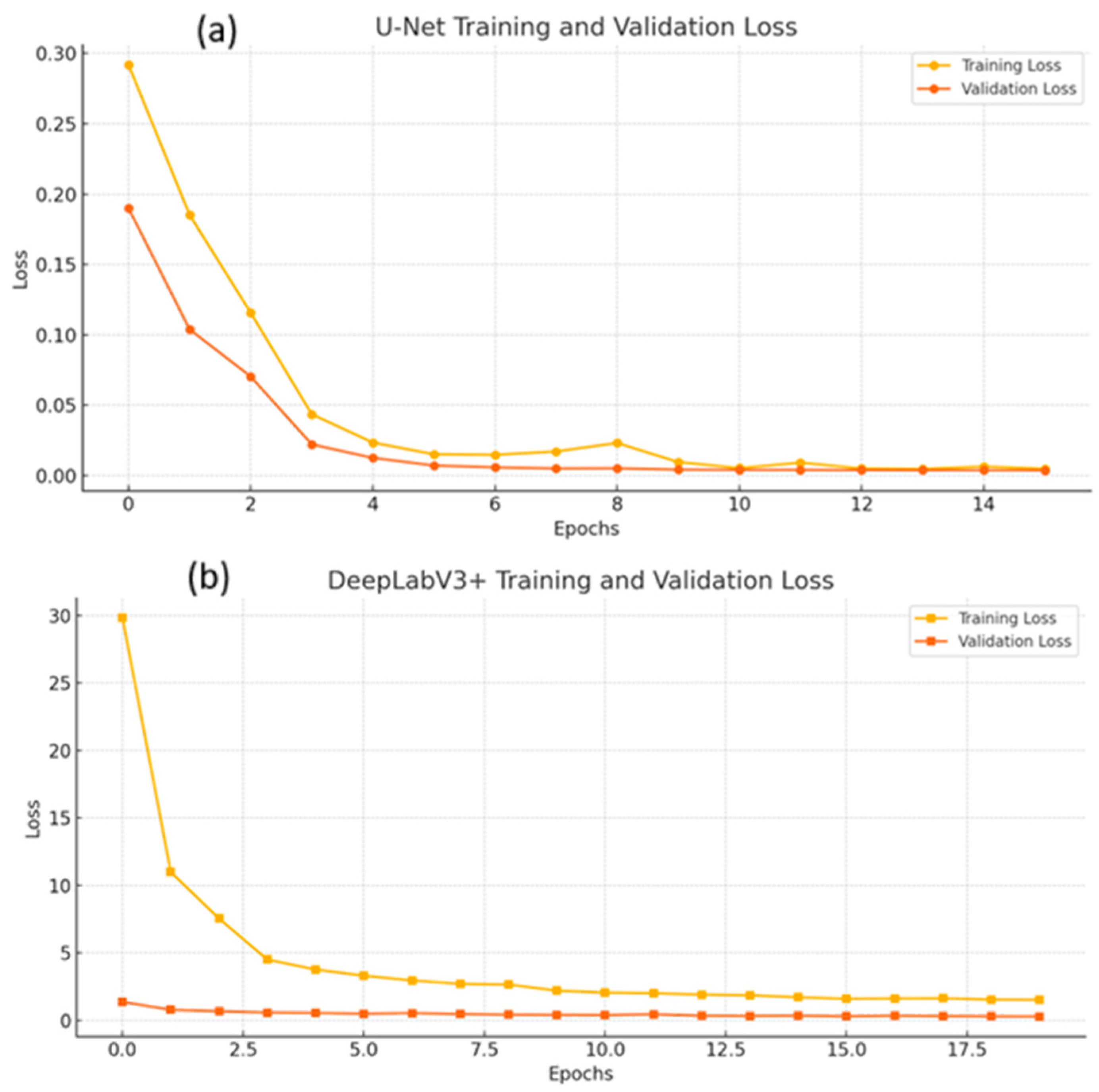
During training on the 2024 Landsat image, both U-Net and DeepLabV3+ models demonstrated excellent and nearly identical performance in terms of precision, recall, and F1 score across land and water classes. The training metrics show that both models achieved F1 scores exceeding 0.997 consistently, indicating strong learning capacity and effective class discrimination at the training stage (see Table 5). Despite the close training performance, an important observation arises from the training and validation loss curves (see Figure 5). Ideally, these curves should decrease concurrently and remain closely aligned, indicating that the model is learning meaningful patterns without overfitting the training data [77,78,79]. U-Net exhibited rapid convergence, reaching a validation loss of 0.0037 and accuracy exceeding 99.8% by epoch 15. The training and validation loss curves were closely aligned, indicating strong generalization and stable learning throughout the training process. In contrast, DeepLabV3+ required more epochs to converge, as seen in Figure 5. Despite starting with a high training loss (29.81) and the larger gap between training and validation losses in early epochs, the model gradually improved and achieved a validation loss of 0.2948 by epoch 20. The trajectory reflects slower learning but eventual stability. However, its final validation loss remained higher compared to U-Net, which may indicate mild overfitting tendencies, where the model fits the training data well but generalizes less effectively to unseen data.
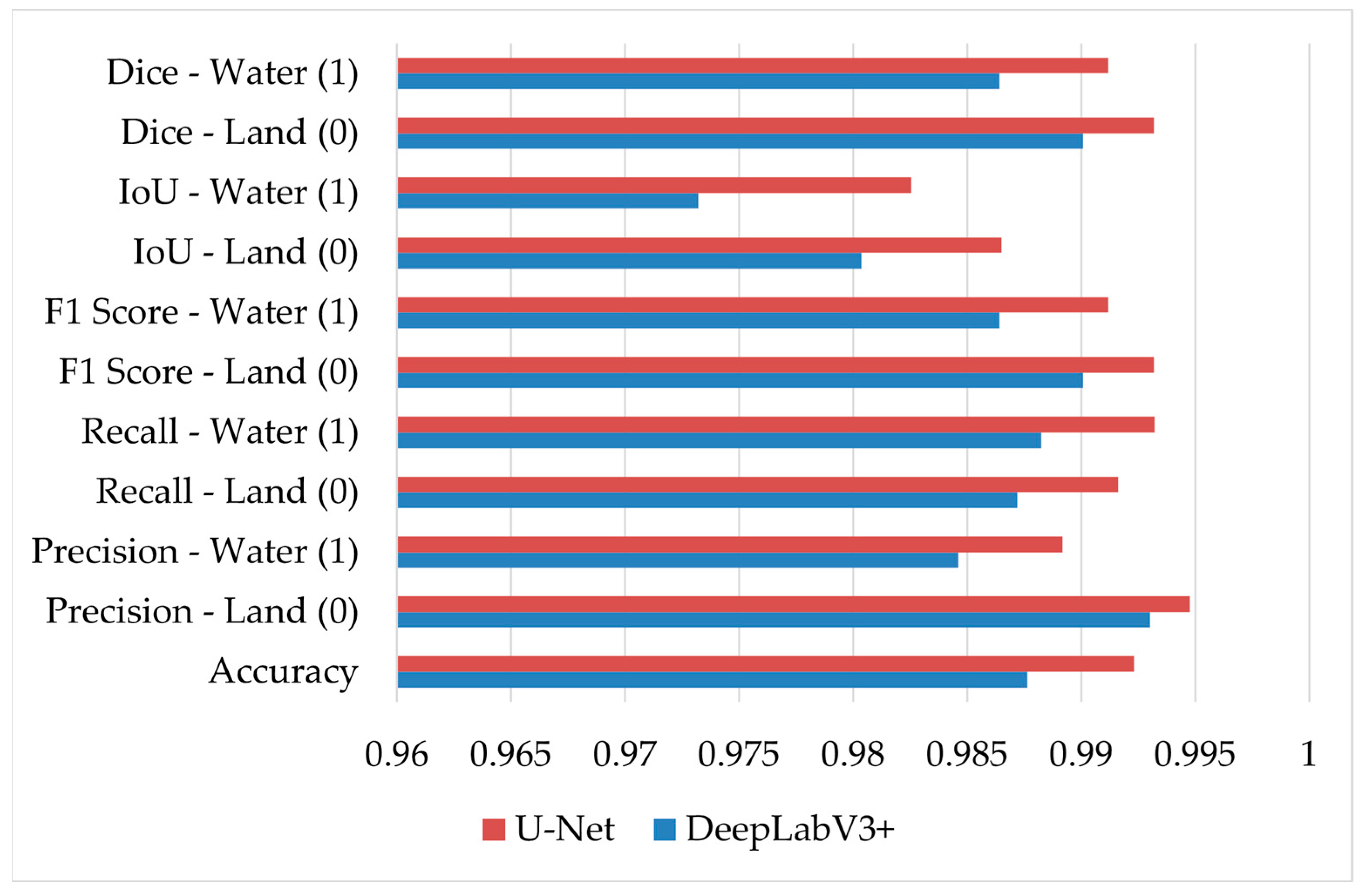
Subsequently, both models were tested on the independent 2018 Landsat image (Figure 6). Evaluation metrics, including precision, recall, F1 score, accuracy, and IoU, were computed for both land and water classes. Results (Figure 6) showed very slight differences in favor of U-Net across all metrics, reaffirming its marginally better generalization capability in the test scenario.
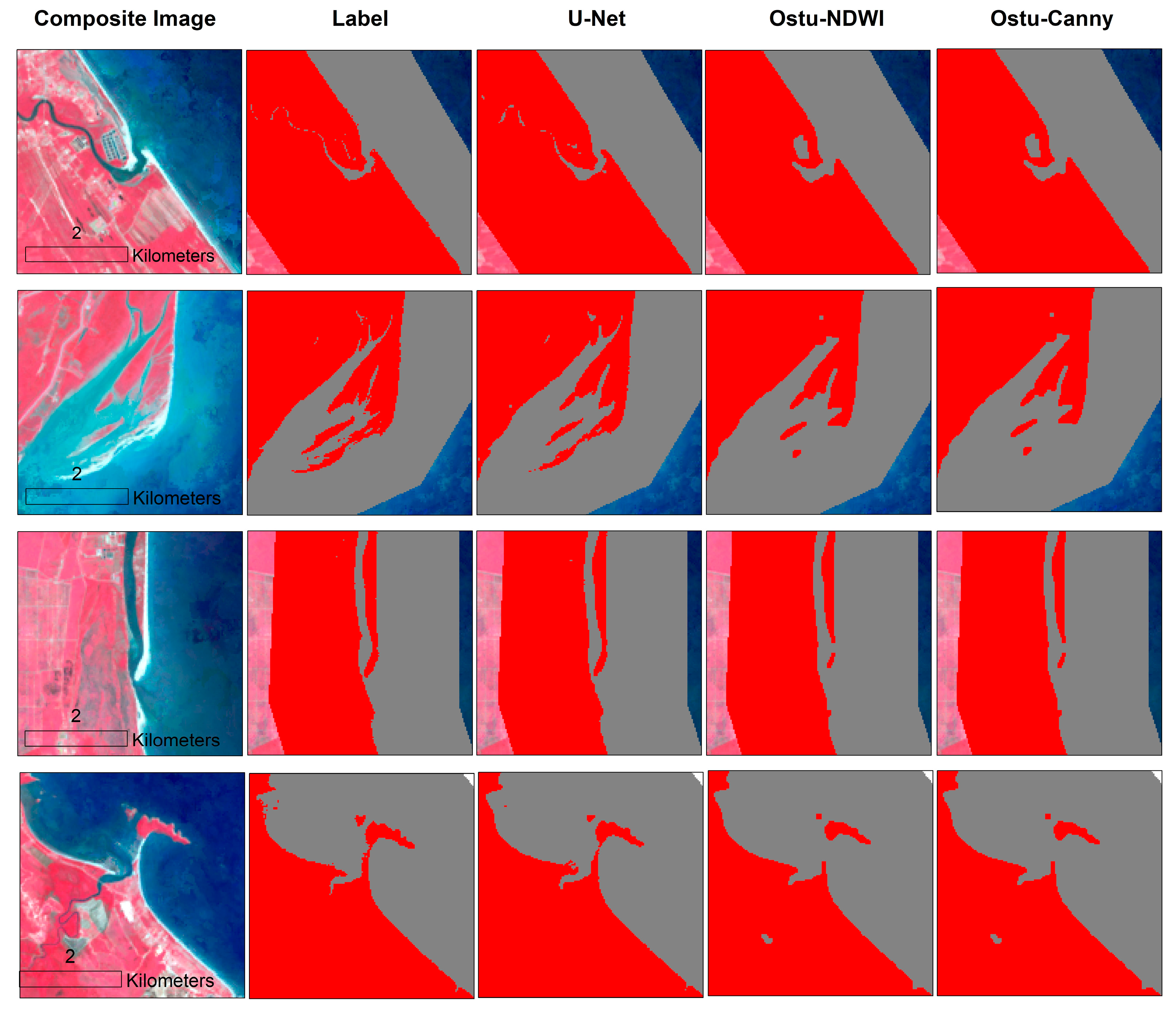
We also compare U-Net derived results with traditional non-DL baseline (NDWI-Otsu and Canny-Otsu). Both baselines performed reasonably, with NDWI–Otsu capturing the bulk class separation and Canny–Otsu improving edge sharpness. However, the CNNs outperformed baselines across all pixel metrics, with U-Net showing the highest mean IoU and F1 (see Table A1 in Appendix A).

4.2. Visual Comparison

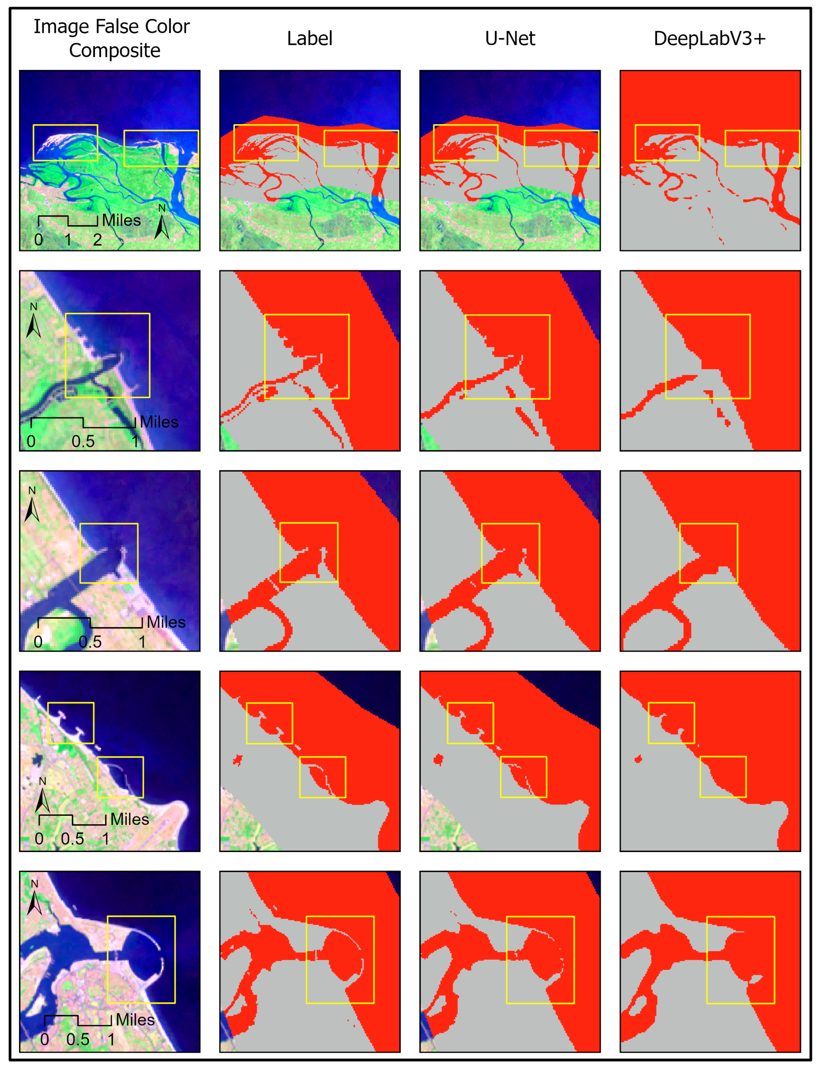
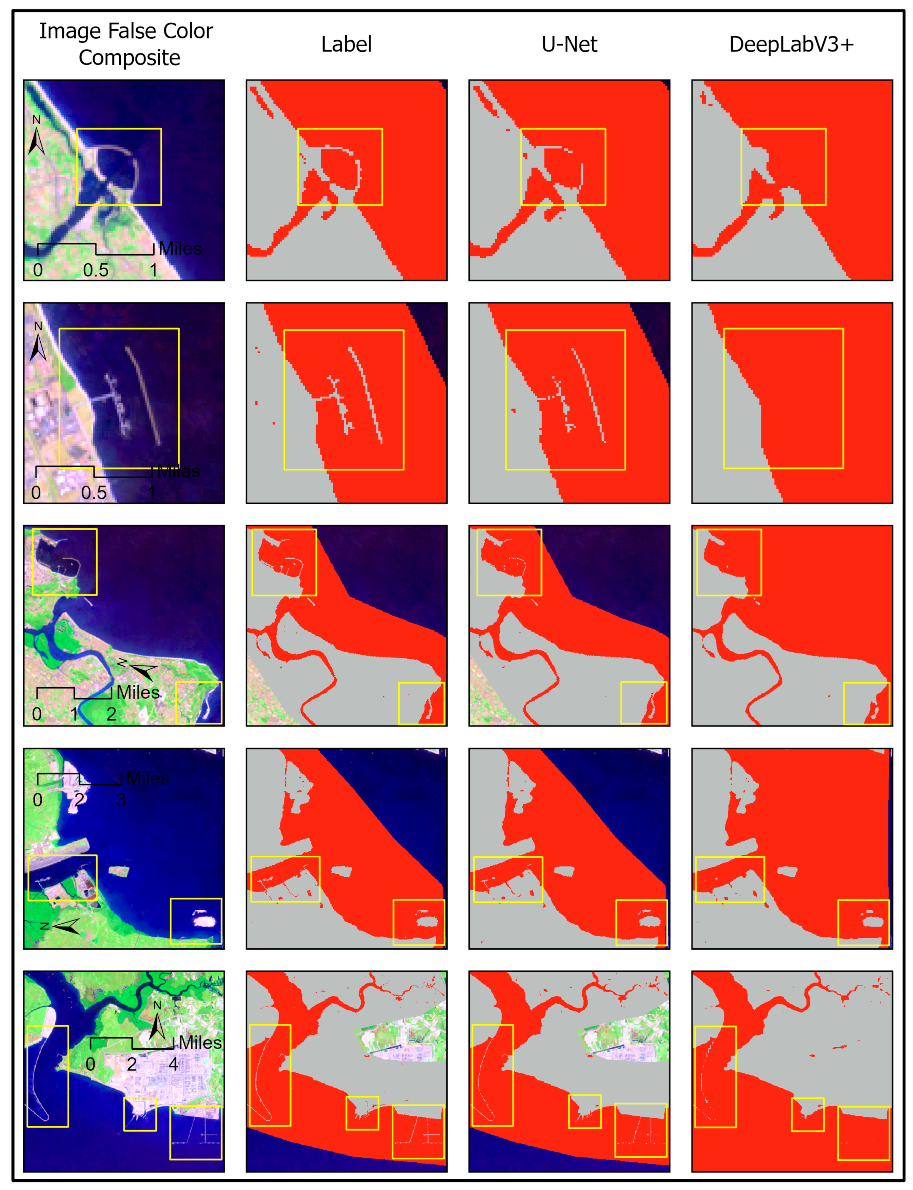
Although the numerical metrics showed very close performance, these indicators alone may not be sufficient to demonstrate the differences between these models. To visually demonstrate the effects of the models, Figure 7 and Figure 8 display the visual inspection of classification results across varied coastal areas. To facilitate observation, the parts with significant differences are marked with rectangular boxes. Although the mIoU of each model is above 97%, there are still significant differences in the actual segmentation results of land and sea. U-Net’s segmentation results displayed more detailed and sharper shoreline boundaries than DeepLabV3+. In regions with intricate shoreline boundaries, such as narrow inlets, estuaries, groynes, and breakwaters, the U-Net model consistently preserved finer geometric details. It effectively maintained spatial fidelity, minimizing edge smoothing and segmentation fragmentation. In contrast, DeepLabV3+, while generally consistent, showed some smoothing effects around curved and narrow shoreline sections, leading to a slight loss of fine-scale features. Moreover, in sediment-heavy or turbid water zones, U-Net exhibited more consistent water delineation, avoiding the overprediction observed in DeepLabV3+. Such visual differences, though subtle, are crucial when classifying shoreline boundaries from medium-resolution sensors like Landsat, where edge precision plays a pivotal role in subsequent spatial analyses, such as DSAS-based shoreline change detection.
Based on both quantitative evaluation metrics and qualitative visual inspection, the U-Net model was selected as the optimal architecture for the subsequent extraction of shorelines across all selected years. While DeepLabV3+ demonstrated strong performance, the differences in accuracy, precision, recall, and F1 score compared to U-Net were marginal. However, U-Net’s faster convergence during training, lower validation loss, and superior ability to preserve fine shoreline details in complex coastal environments provided a decisive advantage.

4.3. Shoreline Change Analysis (DSAS)

DSAS was utilized in this study to determine change rates in the shoreline. Two distinct statistical methods were employed, namely, distance and rate, to estimate the changes along the coastline. The LRR is used to describe the shoreline change rate, while the SCE and NSM represent the distance. At each transect, the SCE was calculated as the difference between the shoreline that was farthest from and closest to the baseline. It estimated the largest distance between all shorelines without considering the specific year of the shoreline. This helped assess the overall change in shoreline movement across all shoreline positions. In contrast, the NSM provided a measure of the separation between the earliest and most recent shorelines, representing the effective change in distance. It indicated the total distance between the oldest and most recent shorelines, i.e., in our case, 1990 and 2024, respectively. While SCE and NSM provided insights into shoreline distance, their findings did not reveal the speed at which the shoreline shifts. To analyze the rate of change, the LRR method was applied. It calculates the average annual rate of change at each transect using all available shoreline positions, offering a statistically robust estimate of long-term trends.

Overall Shoreline Dynamics (1990–2024)

The study area covers the coastal regions of four Malaysian states: Kelantan, Terengganu, Pahang, and Johor. The overall statistics for the study area (Table 6) reveal a relatively high level of shoreline stability, with approximately 40.1% of transects showing no significant change in position. However, the coastal areas still experience substantial erosion and accretion, particularly in regions exposed to monsoon winds and strong tidal currents. The mean SCE, which measures the total horizontal displacement of the shoreline, ranges from 60 to 256.4 m, indicating different levels of shoreline variability across the study area. The maximum SCE values ranged from 2034.2 m in Kelantan to 2061 m in Pahang, highlighting areas of significant change. The NSM values provide insight into whether the coastline has been advancing or retreating over the study period. The mean NSM for erosion across the entire study area was recorded as −23.9 m (22%), while accretion was observed to be 59 m (41%), indicating that shoreline advance has been a dominant trend throughout the study area. The maximum NSM was recorded at −1885.4 m in Kelantan, reflecting the extent of shoreline retreat, while the maximum accretion was recorded at 2028.1 m in Pahang, indicating substantial shoreline growth. The LRR, which calculates the annual long-term rate of shoreline change, further corroborated these findings. The results indicated a stronger trend of accretion than erosion across most states, although significant erosion was observed in certain areas. The mean LRR values for each region reveal a general trend of shoreline advancement or retreat. The mean LRR for erosion was highest in Kelantan (−2.9 m/year), followed by Pahang (−1.24 m/year), while the positive value of LRR was found to be higher in Johor and Pahang, where accretion was more prevalent.
Overall, the analysis reveals a dominant trend of shoreline advance across the study area, with 41.1% of transects showing accretion and a relatively lower percentage of transects experiencing erosion. While Kelantan exhibited significant erosion, Johor and Pahang showed considerable shoreline growth. The stability observed in 40.1% of the transects indicates that large portions of the coastline have remained relatively unchanged, with this stability likely influenced by a mix of natural factors (such as sediment transport and tidal patterns) and human interventions (such as coastal protection measures or land use changes).

4.4. Spatial Distribution of Shoreline Dynamics

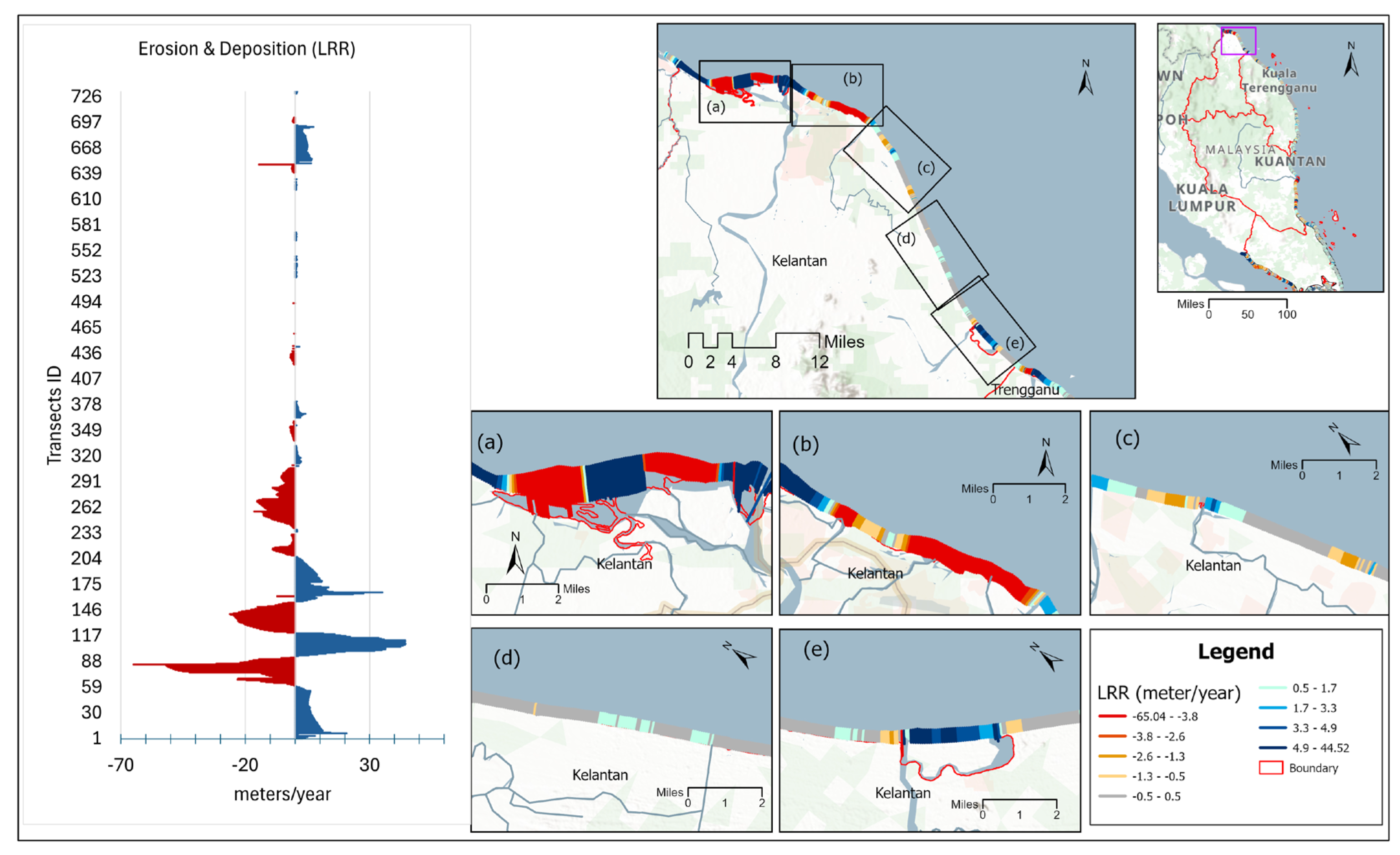
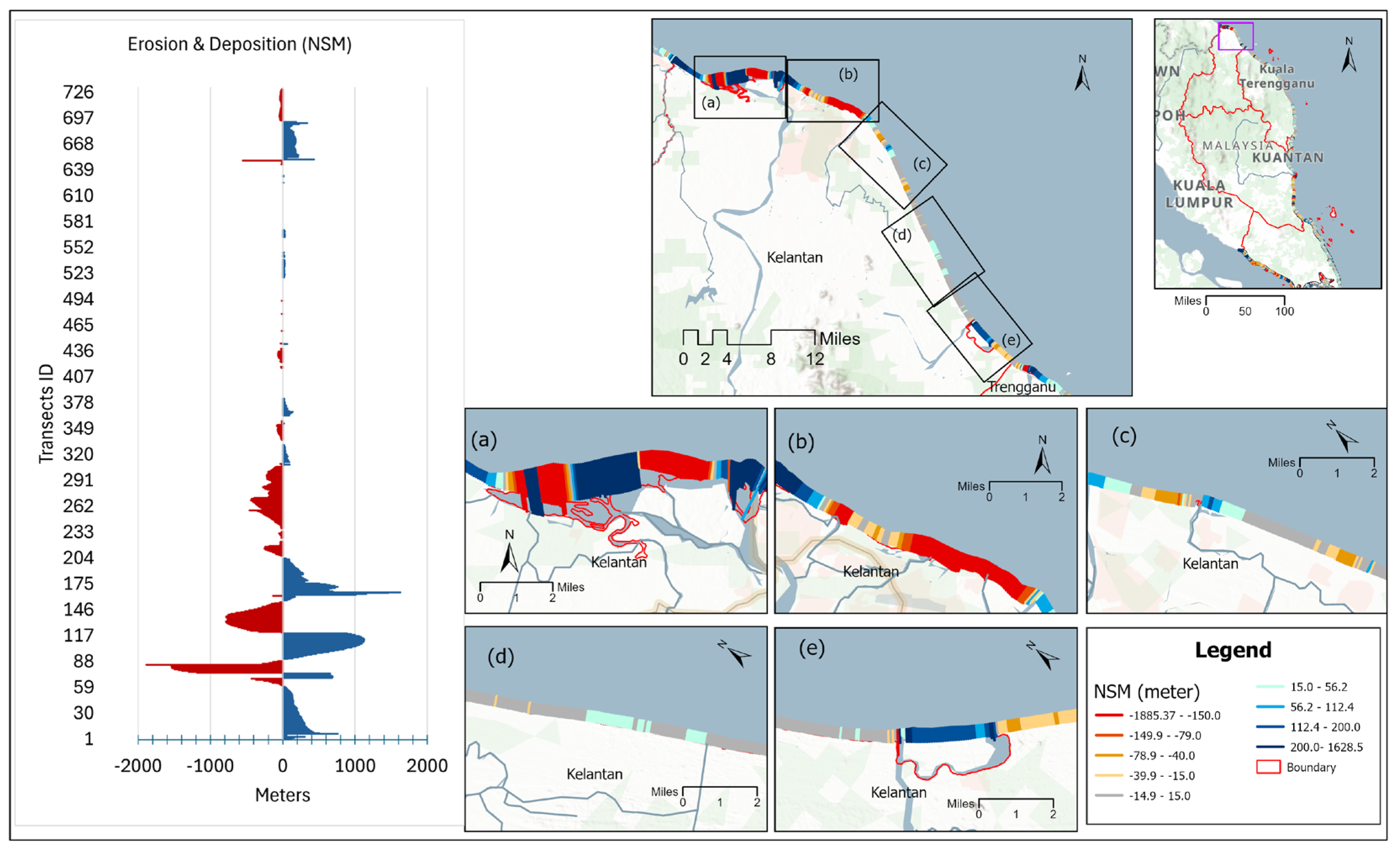
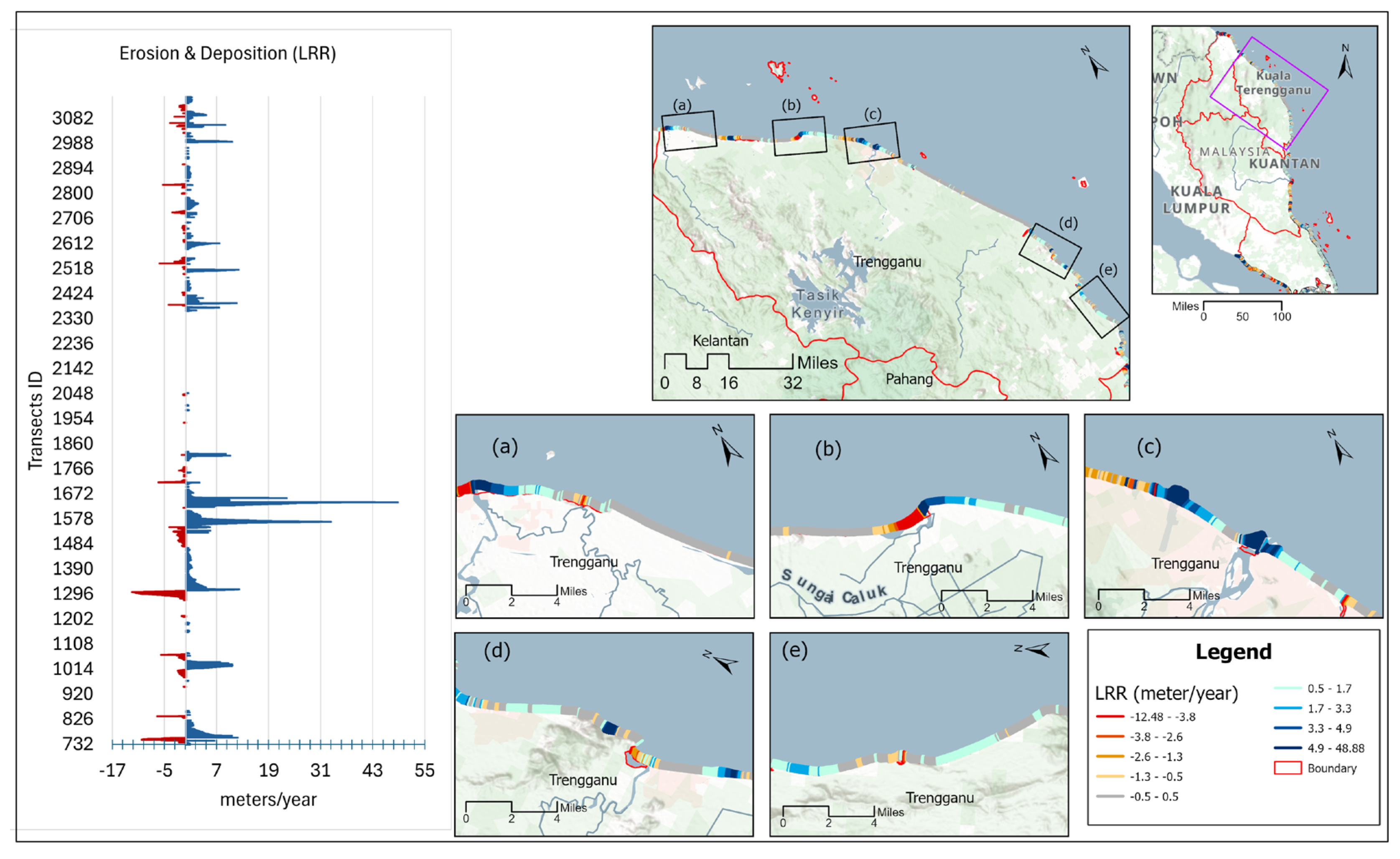
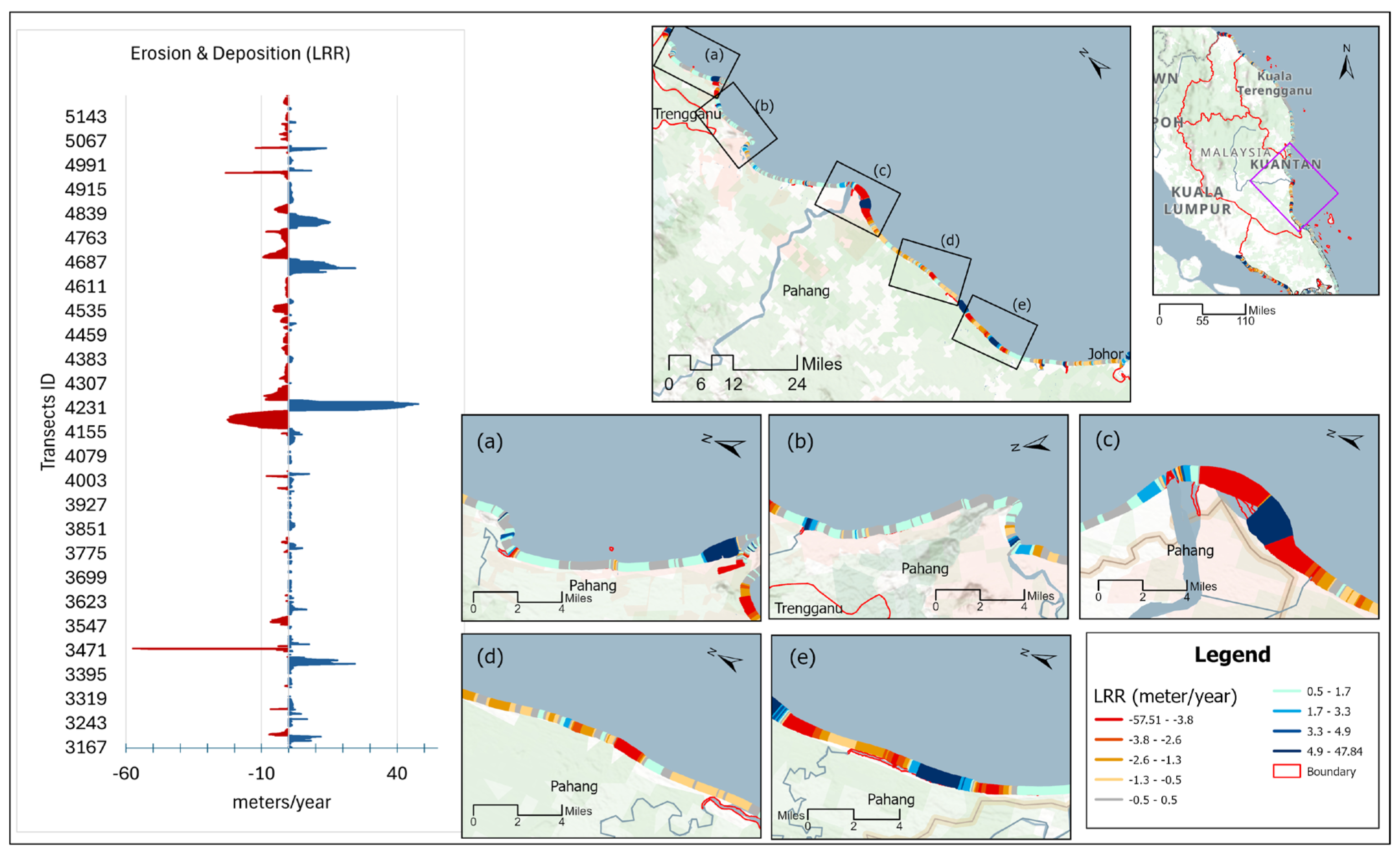
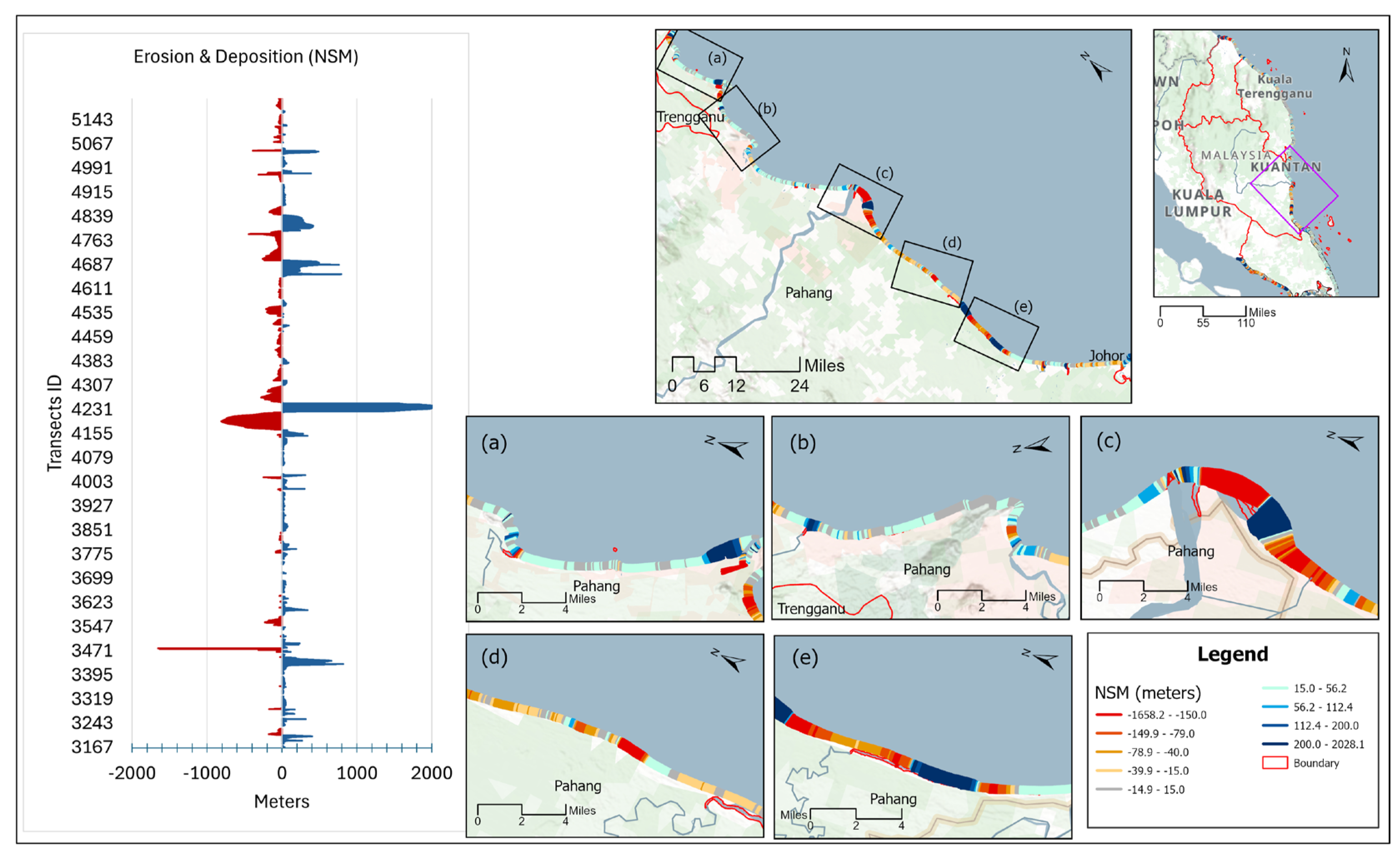
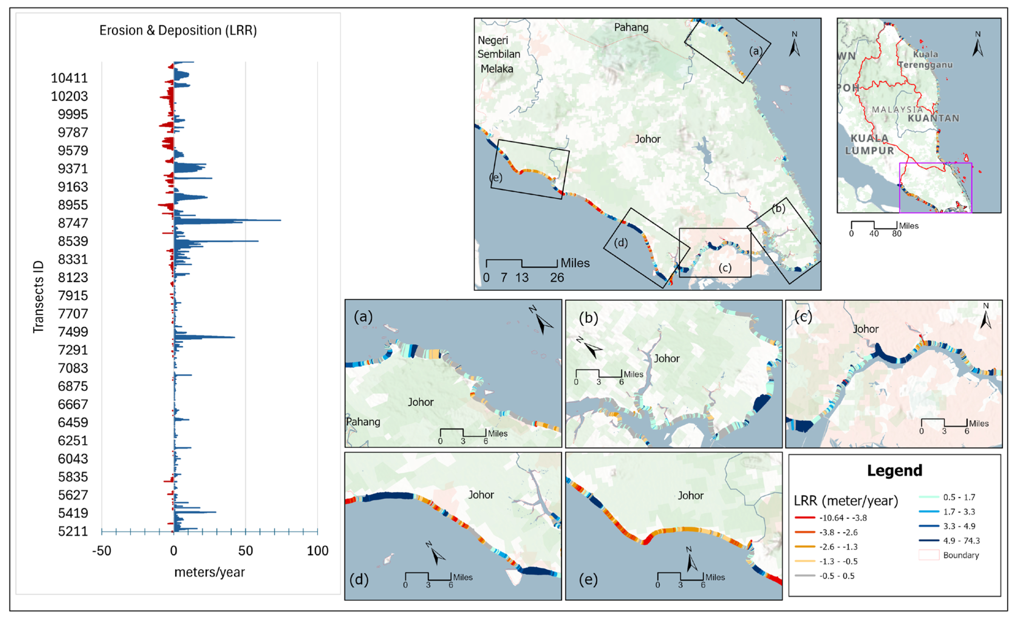
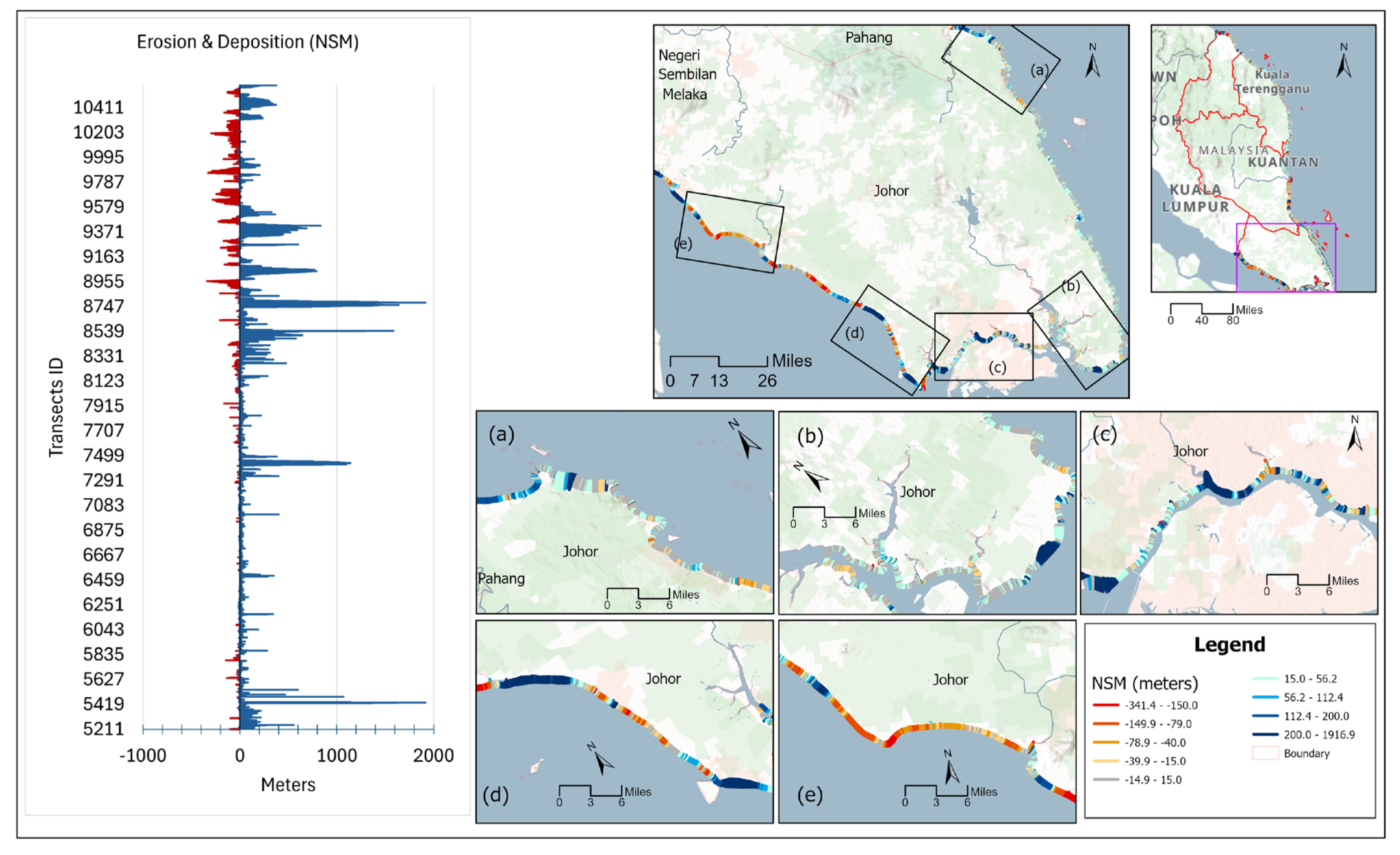
To complement the statistical outputs of the shoreline dynamics, spatial distribution maps of LRR and NSM were generated for each of the four coastal states—Kelantan (Figure 9 and Figure 10), Terengganu (Figure 11 and Figure 12), Pahang (Figure 13 and Figure 14), and Johor (Figure 13 and Figure 14). These maps were developed to visualize shoreline behavior at the transect level, providing an intuitive understanding of how and where the coastlines have either advanced or retreated over the 34-year study period (1990–2024). NSM maps illustrate the net horizontal displacement of the shoreline from the earliest to the most recent year, while the LRR maps depict the average annual rate of change derived through a least-squares regression across all shoreline positions. Each map employs a classified color symbology to represent both the magnitude and direction of shoreline change. For both NSM and LRR maps, warm colors (red, orange, and yellow) indicate erosion (negative values), while cool colors (light blue to dark blue) represent accretion (positive values). Specifically, red denotes the highest erosion, and dark blue signifies the highest accretion. The gray color is used to highlight relatively stable areas, where minimal shoreline movement occurred over the study period. This neutral tone helps distinguish zones with negligible change from those undergoing significant transformation. This visual gradient helps convey not only the extent of change but also highlights the spatial variability in coastal dynamics across different segments of each state’s shoreline.

4.4.1. Kelantan Coast

The Kelantan coastline displayed the most dynamic shoreline behavior among the four states studied. It exhibited intense patterns of both erosion and deposition. The LRR analysis showed that segments of the coast were subjected to severe erosion, with rates reaching up to −64.9 m/year, particularly near the estuarine zones of Kota Bharu. While certain areas experienced strong accretion at a maximum rate of +47.6 m/year. The NSM in Kelantan ranged from −1885.4 m (maximum erosion) to +1628.5 m (maximum accretion), indicating drastic landward and seaward shifts in the shoreline between 1990 and 2024. Figure 9 and Figure 10 revealed a dominant erosional trend along the northernmost section (Figure 9a,b and Figure 10a,b), especially around Tumpat, while southern stretches (Figure 9d,e and Figure 10d,e) exhibited a mix of moderate deposition and relatively stable conditions, possibly influenced by sediment-laden fluvial systems and shallow estuarine formations.

4.4.2. Terengganu Coast

The Terengganu coastline showed relatively more moderate shoreline dynamics, characterized by less extreme values in all three metrics. The LRR values varied from −15.6 m/year in erosional zones to +52.1 m/year in accretional sectors. The NSM values ranged from −364 m and +1183 m, reflecting a spatially heterogeneous shoreline adjustment, albeit less dramatically than in Kelantan or Pahang. Shoreline advancement was notably higher in semi-enclosed coastal embayments, while erosion was prevalent near more exposed headlands. Notably, segments near Bukit Keluang (Figure 11a and Figure 12a) displayed a balanced pattern of erosion and accretion, influenced by both natural forces and engineered interventions such as breakwaters and revetments. The central portion of Terengganu’s coast (Figure 11c and Figure 12c), especially around Kuala Terengganu, exhibited a balanced trend with pockets of stable, retreating, and advancing shoreline. The presence of long accreting stretches in Panels c, d, and e indicates depositional environments, likely supported by riverine sediment input and moderate wave energy, as documented by Zulfakar et al. (2020) [80]. Yet, erosion hotspots persisted near headlands and urbanized stretches, consistent with observed spatial stress patterns due to development pressure.

4.4.3. Pahang Coast

Pahang exhibited one of the widest ranges of shoreline dynamics in the study area. The LRR statistics revealed both the highest erosion rate of −58 m/year and the highest accretion rate of +48 m/year. The NSM values similarly recorded extremes from −1658.2 m to +2028.1 m, marking some of the most substantial changes observed in the study. This duality underscores the diverse coastal processes acting along the Pahang shoreline, which is influenced by river discharge, longshore sediment transport, and wave refraction. Critical erosion was observed particularly near river mouths, such as Pahang river near Pekan (Figure 13c and Figure 14c), and exposed coastal embayments, such as near Kuantan Port (Figure 13a and Figure 14a), while significant accretion was evident near estuarine environments like Kuantan River mouth (Figure 13b and Figure 14b). Notably, the southern part of Pahang displayed dense deposition zones, indicating deltaic progradation or successful natural sediment trapping such as sandbars near Pantai Nenasi and estuarine features of the river mercung (Figure 13e and Figure 14e). The SCE values in Pahang reached the maximum recorded in this study (Table 4), at 2061 m, reflecting large shoreline deviations that may include both natural fluctuations and permanent morphological changes. These trends highlight Pahang’s status as a dynamically adjusting coastline with segments under persistent transformation.

4.4.4. Johor (East and West Coast)

Compared to the other states, the Johor shoreline displayed relatively dominant accretional trends, with only localized sections affected by erosion. The LRR results indicated a maximum accretion rate of +74.3 m/year and a relatively lower erosion rate not exceeding −11.8 m/year. The NSM results supported this observation, showing weight toward seaward expansion, with the maximum accretion recorded at +1917 m, while erosion reached a more modest −341.4 m. The eastern coastal zone (Figure 15a and Figure 16a), adjacent to Pahang, exhibited a dominance of accretion, indicated by dense blue and navy tones. These areas benefit from sediment inflow from the nearby Endau River mouth and reduced wave energy due to the semi-enclosed coastal configuration.
The stable grey zones interspersed on the eastern coast represent low dynamic segments likely buffered by mangrove belts and low-energy marine environments. Moving southward, the inner estuarine corridors of Johor River and Sungai Pulai (Figure 15c and Figure 16c) display a complex pattern. Strong accretion zones along riverbanks are shown in dark blues, likely due to tidal sediment deposition and land reclamation near Forest City and Puteri Harbour, while nearby red-orange bands signal localized erosion, potentially from channel modification or shoreline hardening activities. Likewise, in the southern segment of Johor bordering the Singapore Strait (Figure 15c and Figure 16c), large portions of the coastline—especially near Danga Bay and Pantai Lido—are experiencing high accretion rates, possibly due to ongoing reclamation and urban waterfront development. In contrast, the western coast of Johor (Figure 15d,e and Figure 16d,e) displays more pronounced erosion, marked by extensive red, orange, and yellow transects, particularly near Muar, Pontian, and the coastal stretch south of Batu Pahat. This erosion-prone segment is more directly exposed to wave energy from the Malacca Strait, and it lacks extensive shoreline protection or natural buffers in several locations. The presence of linear development and fragmented mangrove zones may also contribute to increased vulnerability. Notably, some localized accretion zones still appear near sheltered inlets or behind man-made structures, but these are more limited compared to the east and south coast.

5. Discussion

5.1. Interpretation of Model Performance and Segmentation Accuracy

The comparative evaluation of U-Net and DeepLabV3+ revealed that both models are highly competent in shoreline segmentation, achieving F1 scores exceeding 0.997 across land and water classes during training and over 0.96 on independent test data (2018 Landsat). However, despite the similar numerical performance, U-Net demonstrated a slight edge over DeepLabV3+ in terms of generalization and spatial precision, particularly at shoreline boundaries. This finding aligns with prior studies [81,82], which emphasize that while DeepLabV3+ offers efficient multiscale feature extraction and is often favored for its ability to capture complex contextual information through atrous spatial pyramid pooling, U-Net excels in retaining edge fidelity due to its symmetric encoder–decoder structure with skip connections, especially when limited data, high precision localization requirements, and constrained computational resources are involved [31,83,84,85]. Visual inspection further confirmed these observations: U-Net preserved finer geometric shoreline details, especially in areas with narrow inlets, estuaries, or curved coastlines, where DeepLabV3+ tended to smooth over boundary transitions. This qualitative advantage is supported by studies such as Mahmoud. et al. (2025) [31], who reported that a standard U-Net outperformed their customized BDCN-UNet architecture (tailored for edge enhancement) in terms of mean IoU, particularly when trained on clear, well-prepared coastal image datasets. Other studies [60,86,87,88,89] also support the notion that marginal performance gaps in numerical metrics may mask critical differences in boundary quality, which are pivotal in applications like shoreline change detection. Furthermore, the faster convergence and lower validation loss of U-Net during training (as seen in Figure 5) indicate its training stability and learning efficiency, which is especially beneficial in medium-resolution datasets like Landsat. As a result, U-Net was selected as the primary model for historical shoreline extraction across the Malaysian coastline. These findings reiterate that model selection for shoreline extraction should not solely rely on accuracy metrics but also consider practical outcomes such as edge sharpness, generalizability to unseen data, and performance under complex coastal morphologies. In this regard, U-Net remains a robust and deployable choice for operational shoreline monitoring.
Our benchmarking confirms the practical value of reporting CNN results relative to non-DL baselines. While NDWI–Otsu remains a strong low-effort separator and Canny–Otsu sharpens edges, both show higher shoreline-position error and greater sensitivity to turbidity and mixed pixels than U-Net. These gaps are important because DSAS rates (NSM/LRR) depend on planimetric consistency: small boundary distortions can inflate per-transect variance. The CNN’s lower positional error and better retention of fine geometry therefore translate to more stable DSAS trends.

5.2. Evaluation of Long-Term Shoreline Change Trends

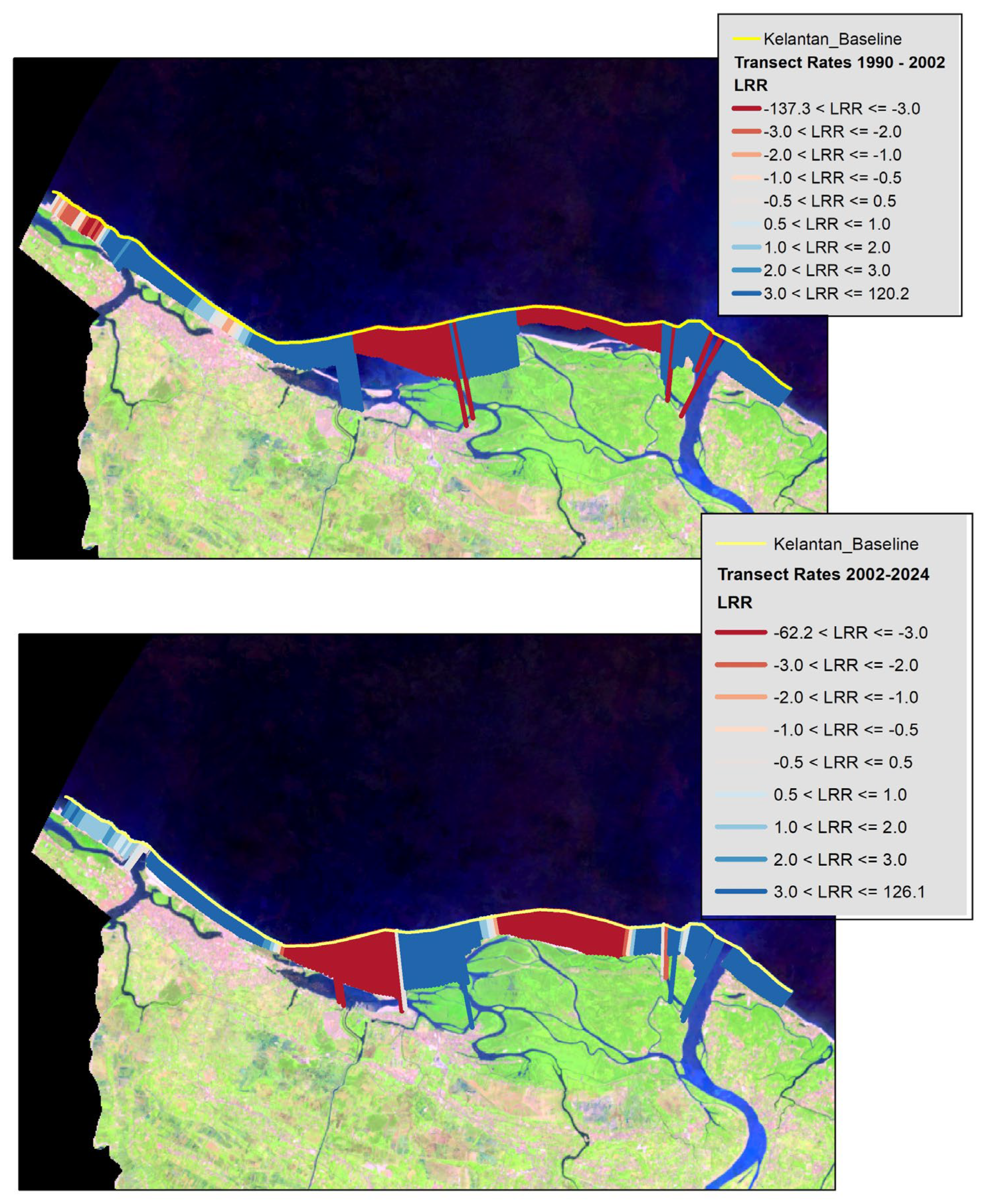
The DSAS-based multidecadal shoreline change analysis along Peninsular Malaysia’s eastern and southern coastlines revealed clear and measurable patterns of accretion, erosion, and stability over the period from 1990 to 2024. Overall, 41.1% of the transects exhibited accretion, 22.5% showed erosion, and 36.4% remained relatively stable, affirming a dominant trend of shoreline advancement across the study area. Among the four states studied, Kelantan emerged as the most dynamic region, with the highest rates of both erosion and accretion. This aligns with prior studies that documented episodic sedimentation in Tumpat (e.g., Pantai Geting) and severe retreat near Kota Bharu (e.g., Pantai Cahaya Bulan) during recent decades [62]. In our analysis, the maximum shoreline retreat (NSM: −1885.4 m) was recorded in Kelantan, while the highest erosion rate (LRR: −64.9 m/year) also occurred in this region. These values reflect the influence of strong northeast monsoon waves, sediment imbalance, and tidal surges that affect the open, estuarine-dominated coastline. However, segmented DSAS results (see Figure A2 in Appendix A) indicate that this extreme erosion was not sustained uniformly over the entire study period. For example, the same hotspot transects exhibited a LRR of −137.3 m/year during 1990–2002, which decreased to −60.3 m/year during 2002–2024, suggesting an initial adjustment phase followed by partial recovery. This pattern supports the interpretation that the observed extremes were episode-limited rather than indicative of a persistent long-term trend. The early 1990s erosion pulse likely coincided with the construction of breakwaters at Kuala Kemasin (1989–1991), which disrupted the prevailing littoral drift and induced downdrift erosion north of the structure [36]. Additionally, high-energy Northeast Monsoon events and major floods (e.g., 2000, 2014) are documented drivers of short-term coastal retreat along Malaysia’s east coast; in Kelantan, this episodic forcing plausibly amplified recession, while subsequent nourishment and revetment works near Pantai Cahaya Bulan contributed to recent stabilization [36,90,91,92,93,94,95].
Terengganu showed more moderate shoreline dynamics from 1990 to 2024, with fewer transects experiencing extreme erosion or accretion compared to Kelantan or Pahang. Notably, the NSM and LRR values indicated relative stability along significant portions of the coastline, especially in central Terengganu, while localized erosion and accretion zones persisted near river mouths and urban centers. However, previous studies [91,96,97,98,99] presented a contrasting narrative. For example, Abdul Rahim et al. (2023) [91] highlighted that several beach segments such as Pantai Rusila, Batu Buruk, and Menggabang Telipot in Kuala Terengganu had been classified under high coastal vulnerability due to intense monsoonal wave activity and anthropogenic pressures, including sand dredging and port development. The observed moderation in our results aligns with recent mitigation measures. The construction of breakwaters, revetments, and a groyne-like airport runway extension has significantly altered local hydrodynamics. Ariffin et al. (2018) [96] noted that after the 2010 airport extension, a clear shift occurred: the updrift areas experienced enhanced erosion due to sediment blockage, while downdrift regions recorded notable accretion due to sediment trapping behind the structure. Furthermore, the implementation of a beach nourishment program (a series of coastal protection structures, including groynes and breakwaters), particularly near Universiti Malaysia Terengganu (UMT) and Tok Jembal, appears to have contributed to the observed shoreline stability in these areas. The construction of these structures in 2016 significantly altered shoreline behavior: zones that had experienced severe erosion during 2004–2016 began to exhibit positive accretion between 2016–2017 [80]. However, studies caution that the apparent accretion at UMT may be more a result of these interventions rather than a natural sedimentary process, highlighting the importance of continued monitoring and integrated coastal zone management [35]. Overall, while our DSAS-based analysis captures a recent trend toward moderate shoreline dynamics in Terengganu, past literature and structural development records underscore the region’s historical vulnerability and the critical role of human interventions in shaping current shoreline conditions. This reinforces the need to distinguish between natural recovery and engineered stability in coastal trend evaluations.
Pahang exhibited one of the broadest ranges of shoreline variation in our study, with both high erosion rates (−58 m/year) and high accretion rates (+48 m/year) along different sections. Particularly active zones were found near river mouths (e.g., Pahang River, Kuantan Port), where scour and sediment deposition cycles contribute to significant morphological adjustments. The studies by Mohd, F.A et al. (2018) and (2019) [100,101] also identified Tanjung Agas and areas south of Kuantan as key erosion-prone and accreting sectors, respectively, echoing the patterns captured in our LRR and NSM outputs. However, a notable finding from our analysis—absent in prior studies—is the presence of a long, continuous erosion-prone stretch located south of the Pahang River, clearly depicted in Figure 13d,e and Figure 14d,e. This southern corridor exhibited some of the highest erosion rates in the state, with several transects exceeding −50 m/year, indicating an actively retreating shoreline that has not been previously documented in the literature. The drivers in this segment are likely a combination of direct monsoonal wave exposure, lack of protective vegetation or structures, and possibly longshore sediment deficit south of the river mouth. Unlike northern urban centers such as Kuantan, which benefit from estuarine sedimentation and localized engineering, this southern corridor appears unprotected and vulnerable yet absent from current mitigation planning and vulnerability assessments. This overlooked erosion zone highlights a critical spatial gap in previous shoreline change assessments and coastal vulnerability mapping for Pahang. It points out the importance of expanding monitoring efforts and mitigation planning beyond well-studied urban and tourism-centric zones (e.g., Cherating–Pekan corridor) to include underrepresented but highly vulnerable segments such as the southern coastal belt below Kuala Pahang.
The Johor coastline presented a predominantly accretional trend, especially along the east coast and southern shorelines. However, the western coast showed localized erosion, especially in areas like Muar and Pontian, which lack natural buffers and face the open Malacca Strait. The eastern coast, extending from Mersing to Desaru, appeared predominantly stable across the entire observation period, with minimal net shoreline movement and low linear regression rates. This observation aligns well with the vulnerability assessment conducted by Ariffin et al. (2023) [14], where the eastern coast of Johor was classified within the least vulnerable zone, due to its relatively unexposed geography and limited anthropogenic interventions. A more dynamic shoreline behavior was observed in the southern region of Johor, which recorded significant accretion rates (with NSM > +120 m in several transects and LRR up to +4.2 m/year). This spatial pattern is strongly documented by Wang et al. (2019) [102]. Their analysis using multi-temporal Landsat imagery from 1973 to 2017 identified over 40 km2 of reclaimed land, driven by urban expansion, port development, and land conversion policies under Iskandar Malaysia initiatives. This large-scale coastal modification offers a credible explanation for the observed long-term accretion in our DSAS results. Interestingly, a contrast arises when comparing our results with Zulkifle et al. (2024) [103], who assessed shoreline dynamics at 12 locations along the Johor Strait from 2018 to 2022. Their findings indicated that 10 out of 12 sites were experiencing significant erosion, including Danga Bay to Stulang corridor. However, this temporal mismatch could explain the discrepancy; while their study captured short-term erosional fluctuations (possibly due to intensified monsoonal cycles or construction disturbance), our study encapsulates a 34-year net shoreline evolution, where cumulative sediment deposition and coastal stabilization efforts may have offset short-term losses. Furthermore, reclamation-induced sedimentation and hydrodynamic alterations could mask erosional episodes over longer periods. Another localized pattern of erosion was visible at Tanjung Piai, particularly on its eastern flank, whereas the western side exhibited clear accretion. This bifurcated behavior aligns closely with the findings from Awang et al. (2014) and Manaf et al. (2018) [104,105], which also reported eastern Tanjung Piai to be more erosion-prone due to wave reflection and littoral drift, while the west remained protected by extensive mangrove buffers and low wave energy. These site-specific dynamics validate our map interpretations and point to the effectiveness of natural vegetation and wave sheltering in shoreline preservation. Overall, the Johor coastline reflects a complex interplay of natural and anthropogenic influences. While short-term studies highlight localized erosional threats, our long-term DSAS results present a net accretional trend, especially where reclamation and development projects have reshaped the shoreline. This underscores the importance of integrating temporal context and land use history when evaluating shoreline change and coastal vulnerability.
The observed shoreline dynamics across Peninsular Malaysia result from an interplay of hydrodynamic forces and human interventions. In Kelantan and Pahang, intense northeast monsoon waves, estuarine sediment fluxes, and tidal surges drive severe retreat in exposed sectors, while localized accretion reflects river-mouth deposition [62,100]. In Terengganu, mitigation structures including breakwaters, revetments, and beach nourishment near Universiti Malaysia Terengganu have altered alongshore sediment transport, stabilizing previously erosional zones [35,80]. Johor’s extreme progradation is largely attributable to large-scale reclamation under Iskandar Malaysia, port expansions, and urban land conversions, which collectively generated >40 km2 of new coastal land since the 1970s [106]. Distinguishing these engineered effects from natural sedimentary processes is essential, as the apparent accretion may represent structural trapping rather than sustainable shoreline recovery.
In a global context, the magnitude of shoreline change we observed in Malaysia varies from moderate to extreme. Most of our coastlines experienced changes of only a few meters per year, consistent with global assessments showing <0.5 m/yr as the norm for 75% of sandy beaches [107,108]. However, Kelantan’s maximum retreat rate (−65 m/yr) stands out as one of the highest reported: it is on par with the worst erosion cases in Southeast Asia, such as the mangrove losses in Demak, Indonesia (up to ~−52 m/yr) [109,110]. Even in tropical Australia, which has vast undeveloped coasts, only ~8% of sites see erosion beyond 0.5 m/yr [111], making Kelantan’s hotspot an outlier. On the accretion side, Johor’s +1900 m net advance (due to reclamation) vastly exceeds natural progradation rates (typically +1–2 m/yr in sediment-rich tropical deltas) [112,113]. In Australia, tide-normalized national mapping [111] demonstrates a broad balance of erosion and accretion since 1988, with localized progradation (e.g., up to ~9.8 m yr−1 along mangrove-front coasts in the Gulf of Carpentaria) that is one order of magnitude lower than Johor’s southern progradation where publicly documented reclamation (e.g., Forest City, Johor Strait) provides a direct mechanism for the very high progradation rates [114]—highlighting the role of reclamation and engineered shorelines in our study area. In Indonesia, multi-sensor DSAS analyses along East Java (2000–2019) [115] show deltaic extremes comparable to Malaysia’s: −87.44 to +111.75 m yr−1 near the Bengawan Solo and Brantas/Porong deltas, placing our Kelantan erosion and Johor accretion well within the upper tail of tropical, river-influenced shoreline change rates. These comparisons underscore that, while Peninsular Malaysia’s overall shoreline change rates are in line with global patterns, certain locations have undergone exceptional changes. Our multi-decadal, satellite-derived analysis thus provides valuable evidence of where Malaysian coastlines behave typically versus where they diverge dramatically from global norms.
This evaluation demonstrates that while shoreline advancement has been the overall trend, localized erosion remains a significant hazard in high-energy or unprotected zones. Such insights are crucial for prioritizing mitigation measures and long-term coastal resilience planning.

5.3. Implications for Coastal Monitoring and Management

The integration of deep learning-based shoreline segmentation with DSAS has proven to be a powerful and scalable framework for assessing long-term coastal dynamics in Peninsular Malaysia. The ability to process historical Landsat imagery with automated shoreline extraction not only reduced manual workload but also enhanced the objectivity and consistency of results across diverse geomorphological settings. The findings of this study offer critical spatial insights for coastal planners and environmental managers. Regions such as the southern coastline of Pahang, the western margin of Johor, and parts of Kelantan’s estuarine zones emerged as erosion hotspots requiring urgent attention. Conversely, accretion-dominated sectors, often driven by reclamation or riverine sediment deposition (e.g., southern Johor and Kuantan estuary), necessitate monitoring to understand long-term morphological impacts and ecological shifts. This approach can complement existing national frameworks like the National Coastal Erosion Study (NCES 2015) [116] and support evidence-based interventions, such as the placement of soft-engineering structures, managed retreat zones, or habitat restoration. Furthermore, the deep learning workflow can be adapted to real-time monitoring platforms when coupled with more frequent imagery (e.g., Sentinel-2), facilitating early-warning systems and adaptive coastal resilience planning.
While DSAS is primarily a retrospective tool, when combined with AI-derived shoreline datasets, it can also provide short-term predictive insight. The regression-based metrics (EPR, LRR, WLR) have been used in previous studies to extrapolate shoreline positions by one to two decades (e.g., Harikrishna et al., (2024) [65]), assuming that past drivers remain stationary. In our case, the integration of CNN-extracted shorelines with DSAS offers a consistent multi-decadal baseline from which such projections can be cautiously extended. However, it is important to emphasize that DSAS does not inherently incorporate climate-change processes such as sea-level rise (SLR). To account for this, DSAS-based projections should be combined with external SLR scenarios (e.g., IPCC AR6 regional projections [116]; Le Cozannet et al., 2019 [8]) to adjust future shoreline trajectories. Thus, the AI–DSAS integration provides a valuable platform for near-term shoreline forecasting and identification of erosion ‘hotspots,’ while serving as a complement to more physically based coastal models for long-term planning under sea-level rise.

5.4. Limitations and Future Work

While the study presents a robust analysis of shoreline change, several limitations should be acknowledged. The spatial resolution of Landsat imagery (30 m) may obscure finer shoreline features, especially in narrow estuaries or mangrove-fringed zones. Additionally, cloud coverage and missing scenes may have led to temporal discontinuities in shoreline positioning. The deep learning models, while effective, were trained on a limited number of chips and epochs, which may constrain generalizability under highly turbid or vegetated coastlines. Also, the DSAS methodology primarily captures planimetric change, without incorporating vertical or volumetric beach dynamics.
Future research could address these limitations by:
  • Utilizing higher-resolution satellite imagery (e.g., SPOT, PlanetScope);
  • Conducting seasonal shoreline analysis to capture short-term variability;
  • Applying ensemble deep learning models;
  • Integrating DSAS outputs with hydrodynamic simulations to assess climate change–induced risks (e.g., storm surge, sea-level rise);
  • Extending this framework to evaluate how shoreline change dynamics and model performance vary across contrasting coastal morphologies (e.g., mangrove-fringed coasts, sandy beaches, estuarine environments), as these settings may exhibit distinct responses to hydrodynamic forcing and anthropogenic interventions.
  • Exploring automated shoreline updating systems using cloud computing platforms such as Google Earth Engine;
  • Such advancements will improve both temporal resolution and model reliability, enhancing their value in operational coastal risk management.

6. Conclusions

This study presents a comprehensive, data-driven assessment of long-term shoreline change across the eastern and southern coasts of Peninsular Malaysia from 1990 to 2024. By integrating deep learning-based shoreline extraction (U-Net and DeepLabV3+) with the DSAS methodology, we successfully mapped spatial and temporal trends in erosion, accretion, and stability at a regional scale. Among the four states, Kelantan exhibited the most dynamic shoreline behavior, driven by estuarine processes and monsoonal influences. Pahang showed both extensive erosion (particularly south of Kuala Pahang) and accretion near river mouths. Terengganu, although historically vulnerable, now displays more stable conditions due to the implementation of effective coastal structures. Johor exhibited a predominantly accretional trend, especially in its southern and eastern areas, though localized erosion persists in its western regions. These findings not only align with but also expand upon prior regional studies by identifying new erosion-prone areas, particularly in underrepresented southern Pahang and western Johor, while providing validated evidence of the effectiveness of coastal defense structures in Terengganu and Johor. The integration of AI with geospatial techniques in this study demonstrates significant potential for national-scale coastal monitoring frameworks. Future efforts should focus on enhancing spatial resolution, seasonal monitoring, and coupling with hydrodynamic modeling to better inform coastal zone planning and climate adaptation strategies.

Author Contributions

Conceptualization, A.B.P. and S.K.; methodology, S.K.; software, S.K.; validation, S.K., M.B. and E.H.A.; formal analysis, S.K.; writing—original draft preparation, S.K.; writing—review and editing, A.B.P. and S.B.H.; visualization, M.F.A.; supervision, A.B.P., M.B. and E.H.A.; funding acquisition, A.B.P. All authors have read and agreed to the published version of the manuscript.

Funding

This study was conducted under the Research Intensified Grant Scheme (RIGS) (vote no: 55436) funding provided by the University Malaysia Terengganu Research Fund (DP-UMT).

Data Availability Statement

The raw data supporting the conclusions of this article will be made available by the authors upon request.

Acknowledgments

We are thankful to the Universiti Malaysia Terengganu for providing the facilities for this investigation.

Conflicts of Interest

The authors declare no conflicts of interest.

Appendix A

Table A1. Tested performance metrics of U-Net model against traditional non-DL methods on the 2018 Landsat image.
MetricU-NetNDWI-OtsuCanny-Otsu
Accuracy0.9870.9520.972
Precision—Land0.9930.9970.997
Precision—Water0.9840.9630.963
Recall—Land0.9870.9600.960
Recall—Water0.9880.9570.957
F1 Score—Land0.9900.9840.984
F1 Score—Water0.9860.9800.980
IoU—Land0.9800.9580.968
IoU—Water0.9730.9600.960
Dice—Land0.9900.9840.984
Dice—Water0.9860.9800.980
Visual overlays (Figure A1) illustrate that baselines tend to over-smooth narrow inlets and groyne/jetty tips; Canny–Otsu recovers more curvature than NDWI–Otsu but still breaks continuity in turbid plumes or shadowed pixels. U-Net preserves continuous, crisp shorelines across estuaries and engineered structures, which is critical for DSAS.
Figure A1. Detailed visualization of the segmentation results of U-Net against the non-DL methods on the 2018 Landsat image.
Remotesensing 17 03334 g0a1
Figure A2. Segmented LRR results for Kelantan coast using DSAS. The same hotspot transect shows a deceleration from −137.3 m yr−1 (1990–2002) to −60.3 m yr−1 (2002–2024), suggesting an episode-limited erosion pulse followed by partial recovery.
Remotesensing 17 03334 g0a2

References

  1. Neumann, B.; Ott, K.; Kenchington, R. Strong Sustainability in Coastal Areas: A Conceptual Interpretation of SDG 14. Sustain. Sci. 2017, 12, 1019–1035. [Google Scholar] [CrossRef] [PubMed]
  2. Islam, G.M.N.; Khir, M.F.A.; Patwary, A.K. Environmental Pollution and Value of Ecotourism Resources in the “No-Take” Marine Protected Areas: A Case of Perhentian Marine Park, Malaysia. Sci. Talks 2024, 12, 100399. [Google Scholar] [CrossRef]
  3. Pendleton, L.; Evans, K.; Visbeck, M. We Need a Global Movement to Transform Ocean Science for a Better World. Proc. Natl. Acad. Sci. USA 2020, 117, 9652–9655. [Google Scholar] [CrossRef]
  4. Dhiman, R.; Kalbar, P.; Inamdar, A.B. Assimilating Geospatial and Decision Science: Application to Planning and Management of Urban Coasts. In Advances in Urban Planning in Developing Nations; Routledge: London, UK, 2021; pp. 140–159. [Google Scholar] [CrossRef]
  5. Bamunawala, J.; Ranasinghe, R.; Dastgheib, A.; Nicholls, R.J.; Murray, A.B.; Barnard, P.L.; Sirisena, T.A.J.G.; Duong, T.M.; Hulscher, S.J.M.H.; van der Spek, A. Twenty-First-Century Projections of Shoreline Change along Inlet-Interrupted Coastlines. Sci. Rep. 2021, 11, 14038. [Google Scholar] [CrossRef]
  6. Alvarez-Cuesta, M.; Toimil, A.; Losada, I.J. Reprint of: Modelling Long-Term Shoreline Evolution in Highly Anthropized Coastal Areas. Part 2: Assessing the Response to Climate Change. Coast. Eng. 2021, 169, 103985. [Google Scholar] [CrossRef]
  7. Nicholls, R.J.; Cazenave, A. Sea-Level Rise and Its Impact on Coastal Zones. Science (1979) 2010, 328, 1517–1520. [Google Scholar] [CrossRef]
  8. Le Cozannet, G.; Bulteau, T.; Castelle, B.; Ranasinghe, R.; Wöppelmann, G.; Rohmer, J.; Bernon, N.; Idier, D.; Louisor, J.; Salas-y-Mélia, D. Quantifying Uncertainties of Sandy Shoreline Change Projections as Sea Level Rises. Sci. Rep. 2019, 9, 42. [Google Scholar] [CrossRef]
  9. Aziz, A.F.; Mardi, N.H.; Abdul Malek, M.; Teh, S.Y.; Wil, M.A.; Shuja, A.H.; Ahmed, A.N.; Kumar, P.; Sherif, M.; Elshafie, A. Development of Inundation Maps along East Coast of Peninsular Malaysia Due to Predicted Seaquake from Manila Trench. Appl. Water Sci. 2023, 13, 62. [Google Scholar] [CrossRef]
  10. Dal Barco, M.K.; Furlan, E.; Pham, H.V.; Torresan, S.; Zachopoulos, K.; Kokkos, N.; Sylaios, G.; Critto, A. Multi-Scenario Analysis in the Apulia Shoreline: A Multi-Tiers Analytical Framework for the Combined Evaluation and Management of Coastal Erosion and Water Quality Risks. Environ. Sci. Policy 2024, 153, 103665. [Google Scholar] [CrossRef]
  11. Laignel, B.; Vignudelli, S.; Almar, R.; Becker, M.; Bentamy, A.; Benveniste, J.; Birol, F.; Frappart, F.; Idier, D.; Salameh, E.; et al. Observation of the Coastal Areas, Estuaries and Deltas from Space. Surv. Geophys. 2023, 44, 1309–1356. [Google Scholar] [CrossRef]
  12. Wang, G.; Duan, Z.; Yu, T.; Shen, Z.; Zhang, Y. Analysis of Coastline Changes under the Impact of Human Activities during 1985–2020 in Tianjin, China. PLoS ONE 2023, 18, e0289969. [Google Scholar] [CrossRef]
  13. Dong, W.S.; Ismailluddin, A.; Yun, L.S.; Ariffin, E.H.; Saengsupavanich, C.; Abdul Maulud, K.N.; Ramli, M.Z.; Miskon, M.F.; Jeofry, M.H.; Mohamed, J.; et al. The Impact of Climate Change on Coastal Erosion in Southeast Asia and the Compelling Need to Establish Robust Adaptation Strategies. Heliyon 2024, 10, e25609. [Google Scholar] [CrossRef]
  14. Ariffin, E.H.; Mathew, M.J.; Roslee, A.; Ismailluddin, A.; Yun, L.S.; Putra, A.B.; Yusof, K.M.K.K.; Menhat, M.; Ismail, I.; Shamsul, H.A.; et al. A Multi-Hazards Coastal Vulnerability Index of the East Coast of Peninsular Malaysia. Int. J. Disaster Risk Reduct. 2023, 84, 103484. [Google Scholar] [CrossRef]
  15. Angelini, R.; Angelats, E.; Luzi, G.; Ribas, F.; Masiero, A.; Mugnai, F. A review and test of shoreline extraction techniques. Int. Arch. Photogramm. Remote Sens. Spat. Inf. Sci. 2023, 48, 17–24. [Google Scholar] [CrossRef]
  16. Rostami, E.; Sharifi, M.A.; Hasanlou, M. Shoreline extraction using time series of sentinel-2 satellite images by google earth engine platform. ISPRS Ann. Photogramm. Remote Sens. Spat. Inf. Sci. 2023, 10, 653–659. [Google Scholar] [CrossRef]
  17. Effendi Daud, M.; Ikhmal Siddiq bin Jefri Din, M.; Kaamin, M.; Mokhtar, M.; Ikhmal Siddiq Jefri Din, M.; Helmy Ariffin, E.; Anh Duong, N.; Onn Malaysia Kampus Cawangan Pagoh, H.; Pendidikan Tinggi Pagoh, H.; Panchor, J. Mapping the Shoreline: A Review of Satellite Imagery and Drone-Mapping Based Shoreline Digitization Methods. J. Adv. Res. Appl. Sci. Eng. Technol. J. Homepage 2025, 61, 193–207. [Google Scholar] [CrossRef]
  18. Ennouali, Z.; Fannassi, Y.; Benmohammadi, A.; Al-Mutiry, M.; Masria, A. Shoreline Change Detection along North Sebou–Moulay Bousselham, Based on Remote Sensing Analysis. Reg. Stud. Mar. Sci. 2023, 62, 102935. [Google Scholar] [CrossRef]
  19. Scala, P.; Manno, G.; Ciraolo, G. Semantic Segmentation of Coastal Aerial/Satellite Images Using Deep Learning Techniques: An Application to Coastline Detection. Comput. Geosci. 2024, 192, 105704. [Google Scholar] [CrossRef]
  20. Ramachandran, A.; Sujatha, M.; Alruwais, N.; Alshahrani, H.M. Forecasting Coastal Stability: Digital Shoreline Analysis System and Machine Learning Techniques in Evaluating Impacts of Cyclones. Reg. Stud. Mar. Sci. 2025, 81, 103961. [Google Scholar] [CrossRef]
  21. Blais, M.A.; Akhloufi, M.A. Advances in Remote Sensing and Deep Learning in Coastal Boundary Extraction for Erosion Monitoring. Geomatics 2025, 5, 9. [Google Scholar] [CrossRef]
  22. Yum, S.G.; Park, S.; Lee, J.J.; Adhikari, M. Das A Quantitative Analysis of Multi-Decadal Shoreline Changes along the East Coast of South Korea. Sci. Total Environ. 2023, 876, 162756. [Google Scholar] [CrossRef] [PubMed]
  23. Zhao, Q.; Yu, L.; Du, Z.; Peng, D.; Hao, P.; Zhang, Y.; Gong, P. An Overview of the Applications of Earth Observation Satellite Data: Impacts and Future Trends. Remote Sens. 2022, 14, 1863. [Google Scholar] [CrossRef]
  24. García-Rubio, G.; Huntley, D.; Russell, P. Evaluating Shoreline Identification Using Optical Satellite Images. Mar. Geol. 2015, 359, 96–105. [Google Scholar] [CrossRef]
  25. Ankrah, J.; Monteiro, A.; Madureira, H. Bibliometric Analysis of Data Sources and Tools for Shoreline Change Analysis and Detection. Sustainability 2022, 14, 4895. [Google Scholar] [CrossRef]
  26. Boak, E.H.; Turner, I.L. Shoreline Definition and Detection: A Review. J. Coast. Res. 2005, 2005, 688–703. [Google Scholar] [CrossRef]
  27. Lv, Q.; Wang, Q.; Song, X.; Ge, B.; Guan, H.; Lu, T.; Tao, Z. Research on Coastline Extraction and Dynamic Change from Remote Sensing Images Based on Deep Learning. Front. Environ. Sci. 2024, 12, 1443512. [Google Scholar] [CrossRef]
  28. Park, S.; Song, A. Shoreline Change Analysis with Deep Learning Semantic Segmentation Using Remote Sensing and GIS Data. KSCE J. Civ. Eng. 2024, 28, 928–938. [Google Scholar] [CrossRef]
  29. Qiu, K.; Budde, L.E.; Bulatov, D.; Iwaszczuk, D. Exploring Fusion Techniques in U-Net and DeepLab V3 Architectures for Multi-Modal Land Cover Classification. In Proceedings of the Earth Resources and Environmental Remote Sensing/GIS Applications XIII, Berlin, Germany, 5–8 September 2022; Schulz, K., Nikolakopoulos, K.G., Michel, U., Eds.; SPIE: Berlin, Germany, 2022; p. 33. [Google Scholar]
  30. Handayanto, R.T. Land Cover Segmentation of Multispectral Images Using U-Net and DeeplabV3+ Architecture. J. Ilmu Komput. Inf. 2024, 17, 89–96. [Google Scholar] [CrossRef]
  31. Mahmoud, A.S.; Mohamed, S.A.; Helmy, A.K.; Nasr, A.H. BDCN_UNet: Advanced Shoreline Extraction Techniques Integrating Deep Learning. Earth Sci. Inf. 2025, 18, 187. [Google Scholar] [CrossRef]
  32. Khurram, S.; Pour, A.B.; Bagheri, M.; Ariffin, E.H.; Akhir, M.F.; Hamzah, S.B. Developments in Deep Learning Algorithms for Coastline Extraction from Remote Sensing Imagery: A Systematic Review. Earth Sci. Inf. 2025, 18, 187. [Google Scholar] [CrossRef]
  33. Wu, L.; Ishikawa, S.; Inazu, D.; Ikeya, T.; Okayasu, A. An Automatic Shoreline Extraction Method from SAR Imagery Using DeepLab-V3+ and Its Versatility. Coast. Eng. J. 2025, 67, 106–118. [Google Scholar] [CrossRef]
  34. Amara, R.; Diop, M.; Diop, C.; Ouddane, B. The Senegalese Coastal and Marine Environment. In World Seas: An Environmental Evaluation; Elsevier: Amsterdam, The Netherlands, 2019; pp. 855–873. [Google Scholar]
  35. Bagheri, M.; Akhir, M.F.; Gholami, I.; Wolf, I.D.; Nor, N.N.F.B.M.; Yusoff, I.M.; Rashid, S.M.R.A. Assessing Coastal Erosion Dynamics and Sea Level Rise Impacts on Kuala Nerus and Kuala Terengganu, Malaysia: A Case Study in Climate-Resilient Coastal Management. Epis. J. Int. Geosci. 2024, 48, 255–278. [Google Scholar] [CrossRef]
  36. Rashidi, A.H.M.; Jamal, M.H.; Hassan, M.Z.; Sendek, S.S.M.; Sopie, S.L.M.; Hamid, M.R.A. Coastal Structures as Beach Erosion Control and Sea Level Rise Adaptation in Malaysia: A Review. Water 2021, 13, 1741. [Google Scholar] [CrossRef]
  37. Ariffin, E. Effect of Monsoons on Beach Morphodynamics in the East Coast of Peninsular Malaysia: Examples from Kuala Terengganu Coast. Ph.D. Thesis, Université de Bretagne Sud, Lorient, France, 2017. [Google Scholar]
  38. Rojahan, A.; Ibrahim, I.; Noor, N. Analysis of Rate of Shoreline Changes along the Coastline of Kuala Terengganu. Malays. J. Trop. Geogr. 2022, 48, 64–72. [Google Scholar]
  39. Zuraimi, A.; Rafi, Y.; Dahlan, I.; Fadiah, M. A study of logistics development in the malaysia eastern region: A descriptive analysis. Int. J. Bus. Soc. Res. 2012, 2, 309–321. [Google Scholar]
  40. Ahmad, H.; Abdul Maulud, K.N.; Karim, O.A.; Mohd, F.A. Assessment of Erosion and Hazard in the Coastal Areas of Selangor. Malays. J. Soc. Space 2021, 17, 14–31. [Google Scholar] [CrossRef]
  41. Azizan, N.N.; Abdul Rahim, H.; Adnan, N.A.; Razali, R.; Mohd, F.A.; Ariffin, E.H. Assessment of Shoreline Changes at Northern Selangor Coast, Malaysia Using Digital Shoreline Analysis System (DSAS). J. Adv. Geospat. Sci. Technol. 2024, 4, 79–103. [Google Scholar] [CrossRef]
  42. Ehsan, S.; Begum, R.A.; Nor, N.G.M.; Maulud, K.N.A. Current and Potential Impacts of Sea Level Rise in the Coastal Areas of Malaysia. IOP Conf. Ser. Earth Environ. Sci. 2019, 228, 012023. [Google Scholar] [CrossRef]
  43. Wulder, M.A.; Loveland, T.R.; Roy, D.P.; Crawford, C.J.; Masek, J.G.; Woodcock, C.E.; Allen, R.G.; Anderson, M.C.; Belward, A.S.; Cohen, W.B.; et al. Current Status of Landsat Program, Science, and Applications. Remote Sens. Environ. 2019, 225, 127–147. [Google Scholar] [CrossRef]
  44. Mishra, M.; Acharyya, T.; Chand, P.; Santos, C.A.G.; Kar, D.; Das, P.P.; Pattnaik, N.; da Silva, R.M.; do Nascimento, T.V.M. Analyzing Shoreline Dynamicity and the Associated Socioecological Risk along the Southern Odisha Coast of India Using Remote Sensing-Based and Statistical Approaches. Geocarto Int. 2022, 37, 3991–4027. [Google Scholar] [CrossRef]
  45. Dolan, R.; Fenster, M.; Holme, S. Temporal Analysis of Shoreline Recession and Accretion. J. Coast. Res. 1991, 7, 723–744. [Google Scholar]
  46. Moore, L. Shoreline Mapping Techniques. J. Coast. Res. (JSTOR) 2000, 16, 111–124. [Google Scholar]
  47. Liu, Y.; Yang, J.; He, J.; Chen, X.; Yuan, H.; Peng, X. Roof Segmentation of Remote Sensing Images Based on Improved UNET. In Proceedings of the International Conference on Wavelet Analysis and Pattern Recognition, Adelaide, Australia, 9–11 July 2023; pp. 68–73. [Google Scholar] [CrossRef]
  48. Wang, X.; Hu, Z.; Shi, S.; Hou, M.; Xu, L.; Zhang, X. A Deep Learning Method for Optimizing Semantic Segmentation Accuracy of Remote Sensing Images Based on Improved UNet. Sci. Rep. 2023, 13, 7600. [Google Scholar] [CrossRef] [PubMed]
  49. He, K.; Zhang, X.; Ren, S.; Sun, J. Deep Residual Learning for Image Recognition. In Proceedings of the 2016 IEEE Conference on Computer Vision and Pattern Recognition (CVPR), Las Vegas, NV, USA, 27–30 June 2016; IEEE: New York, NY, USA, 2016; pp. 770–778. [Google Scholar]
  50. Gong, S.; Ball, J.; Surawski, N. Urban Land-Use Land-Cover Extraction for Catchment Modelling Using Deep Learning Techniques. J. Hydroinform. 2022, 24, 388–405. [Google Scholar] [CrossRef]
  51. Chen, L.-C.; Zhu, Y.; Papandreou, G.; Schroff, F.; Adam, H. Encoder-Decoder with Atrous Separable Convolution for Semantic Image Segmentation. In Proceedings of the European Conference on Computer Vision, Munich, Germany, 8–14 September 2018; SpringerLink: Berlin, Germany, 2018; pp. 801–818. [Google Scholar]
  52. Chen, H.; Qin, Y.; Liu, X.; Wang, H.; Zhao, J. An Improved DeepLabv3+ Lightweight Network for Remote-Sensing Image Semantic Segmentation. Complex Intell. Syst. 2024, 10, 2839–2849. [Google Scholar] [CrossRef]
  53. Jun, Z.; Shiqiao, C.; Zhenhua, D.; Yuan, Z.; Chabei, L. Automatic Detection for Dam Restored Concrete Based on DeepLabv3+. IOP Conf. Ser. Earth Environ. Sci. 2020, 571, 012108. [Google Scholar] [CrossRef]
  54. Matin, N.; Hasan, G.M.J. A Quantitative Analysis of Shoreline Changes along the Coast of Bangladesh Using Remote Sensing and GIS Techniques. Catena 2021, 201, 105185. [Google Scholar] [CrossRef]
  55. Kong, D.; Miao, C.; Borthwick, A.G.L.; Duan, Q.; Liu, H.; Sun, Q.; Ye, A.; Di, Z.; Gong, W. Evolution of the Yellow River Delta and Its Relationship with Runoff and Sediment Load from 1983 to 2011. J. Hydrol. 2015, 520, 157–167. [Google Scholar] [CrossRef]
  56. Kandel, I.; Castelli, M. The Effect of Batch Size on the Generalizability of the Convolutional Neural Networks on a Histopathology Dataset. ICT Express 2020, 6, 312–315. [Google Scholar] [CrossRef]
  57. Fernando, K.R.M.; Tsokos, C.P. Dynamically Weighted Balanced Loss: Class Imbalanced Learning and Confidence Calibration of Deep Neural Networks. IEEE Trans. Neural Netw. Learn. Syst. 2022, 33, 2940–2951. [Google Scholar] [CrossRef]
  58. Tyagi, S.; Mittal, S. Sampling Approaches for Imbalanced Data Classification Problem in Machine Learning. Lect. Notes Electr. Eng. 2020, 597, 209–221. [Google Scholar] [CrossRef]
  59. Himmelstoss, E.A.; Henderson, R.E.; Kratzmann, M.G.; Farris, A.S. Digital Shoreline Analysis System (DSAS) Version 5.0 User Guide; Open-File Report; USGS: Reston, VA, USA, 2018.
  60. Azad, S.T.; Moghaddassi, N.; Sayehbani, M. Digital Shoreline Analysis System Improvement for Uncertain Data Detection in Measurements. Environ. Monit. Assess. 2022, 194, 646. [Google Scholar] [CrossRef]
  61. Quang, D.N.; Ngan, V.H.; Tam, H.S.; Viet, N.T.; Tinh, N.X.; Tanaka, H. Long-Term Shoreline Evolution Using DSAS Technique: A Case Study of Quang Nam Province, Vietnam. J. Mar. Sci. Eng. 2021, 9, 1124. [Google Scholar] [CrossRef]
  62. Abd Wahid, M.Z.A.; Osman, M.S.; Setumin, S. Comparative Analysis in Shoreline Changes in Kelantan, Malaysia Using Digital Shoreline Analysis System (DSAS). ESTEEM Acad. J. 2023, 19, 109–117. [Google Scholar] [CrossRef]
  63. Rafferty, S.; Naber, M. An Analysis of Bluff Change along the Pennsylvania Lake Erie Coast: 2007-15 and 2012-15. 2021. Pennsylvania Sea Grant, Pennsylvania State University. Available online: https://pawalter.psu.edu/sites/default/files/resources/Bluff%20Analysis%20Report%20%282021%29.pdf (accessed on 2 September 2025).
  64. Murray, J.; Adam, E.; Woodborne, S.; Miller, D.; Xulu, S.; Evans, M. Monitoring Shoreline Changes along the Southwestern Coast of South Africa from 1937 to 2020 Using Varied Remote Sensing Data and Approaches. Remote Sens. 2023, 15, 317. [Google Scholar] [CrossRef]
  65. Harikrishna, S.; Gurugnanam, B.; Bairavi, S.; Shekar, S. Geospatial Technology Based Shoreline Change Analysis (1992–2022) and Predictive Forecast Modeling for 2032 and 2042, Utilizing DSAS, along the Eastern Coast of India. Kuwait J. Sci. 2024, 51, 100272. [Google Scholar] [CrossRef]
  66. Hamsan, M.A.S.; Zaini Mustapa, M.; Ramli, M.Z. Morphology and sand characteristics at five recreational beaches in Pahang. J. Sustain. Sci. Manag. 2019, 14, 2672–7226. [Google Scholar]
  67. Hayes, M. Barrier Island Morphology as a Function of Tidal and Wave Regime; Leatherman, S.P., Ed.; Academic Press: Columbia, SC, USA, 1979; pp. 1–29. [Google Scholar]
  68. Uti, M.N.; Din, A.H.M.; Yusof, N.; Rasib, A.W.; Hamden, M.H.; Hashim, F.E. Assessment of the Potential of Tidal Range Energy in Malaysian Exclusive Economic Zone (EEZ) Using Multi-Mission Satellite Altimetry Data. Int. J. Geoinformatics 2023, 19, 1–14. [Google Scholar] [CrossRef]
  69. Wong, P.P. Beach Changes on a Monsoon Coast, Peninsular Malaysia. Bull. Geol. Soc. Malays. 1981, 14, 59–74. [Google Scholar] [CrossRef]
  70. Rengarajan, R.; Choate, M.; Hasan, M.N.; Denevan, A. Co-Registration Accuracy between Landsat-8 and Sentinel-2 Orthorectified Products. Remote Sens. Environ. 2024, 301, 113947. [Google Scholar] [CrossRef]
  71. Storey, J.; Choate, M.; Lee, K.; Markham, B.; Morfitt, R.; Müller, R.; Thenkabail, P.S. Landsat 8 Operational Land Imager On-Orbit Geometric Calibration and Performance. Remote Sens. 2014, 6, 11127–11152. [Google Scholar] [CrossRef]
  72. Rengarajan, R.; Choate, M.; Storey, J.; Franks, S.; Micijevic, E. Landsat Collection-2 Geometric Calibration Updates. In Proceedings of the Earth Observing Systems XXV, Online, 24 August–4 September 2020. [Google Scholar] [CrossRef]
  73. Choate, M.J.; Rengarajan, R.; Storey, J.C.; Lubke, M. Geometric Calibration Updates to Landsat 7 ETM+ Instrument for Landsat Collection 2 Products. Remote Sens. 2021, 13, 1638. [Google Scholar] [CrossRef]
  74. USGS. Landsat Levels of Processing|U.S. Geological Survey. Available online: https://www.usgs.gov/landsat-missions/landsat-levels-processing (accessed on 2 September 2025).
  75. Ahmed, M.F.; Halder, B.; Juneng, L.; Farooque, A.A.; Yaseen, Z.M. Remote Sensing-Based Shoreline Change Investigation in Klang Coast and Langkawi Island towards Sustainable Coastal Management. Geomat. Nat. Hazards Risk 2025, 16, 2493226. [Google Scholar] [CrossRef]
  76. Ridzuan, N. Evaluating Coastal Erosion and Accretion Along Batu Ferringhi Beach with Digital Shoreline Analysis System. BIO Web Conf. 2025, 176, 01001. [Google Scholar] [CrossRef]
  77. Goodfellow, I.; Bengio, Y.; Courville, A. Deep Learning; The MIT Press: Cambridge, MA, USA; London, UK, 2016; ISBN 9780262035613. [Google Scholar]
  78. Chollet, F. Deep Learning with Python, 2nd ed.; Manning Publications: Shelter Island, NY, USA, 2021; ISBN 9781617296864. [Google Scholar]
  79. Bengio, Y. Practical Recommendations for Gradient-Based Training of Deep Architectures, 2nd ed.; Springer: Berlin/Heidelberg, Germany, 2012; Volume 7700, ISBN 978-3-642-35289-8. [Google Scholar]
  80. Zulfakar, M.; Akhir, M.; Ariffin, E.; Awang, N.; Yaacob, M.; Chong, W.; Muslim, A. The Effect of Coastal Protections on the Shoreline Evolution at Kuala Nerus, Terengganu (Malaysia). J. Sustain. Sci. Manag. 2020, 15, 71–85. [Google Scholar]
  81. Chueprasert, T.; Udomchaiporn, A.; Intagosum, S. Comparative Analysis of Deep Learning Models for Building Extraction from High-Resolution Satellite Imagery. Curr. Appl. Sci. Technol. 2024, 25, e0260846. [Google Scholar] [CrossRef]
  82. Kalinaki, K.; Malik, O.A.; Ching Lai, D.T. FCD-AttResU-Net: An Improved Forest Change Detection in Sentinel-2 Satellite Images Using Attention Residual U-Net. Int. J. Appl. Earth Obs. Geoinf. 2023, 122, 103453. [Google Scholar] [CrossRef]
  83. Chang, L.; Chen, Y.T. Performance Evaluation and Improvement of Shoreline Detection Using Sentinel-1 SAR and DEM Data. IEEE J. Sel. Top. Appl. Earth Obs. Remote Sens. 2024, 17, 8139–8152. [Google Scholar] [CrossRef]
  84. Lin, H.; Li, L.; Qiang, Y.; Xu, X.; Liang, S.; Chen, T.; Yang, W.; Zhang, Y. A Method for Landslide Identification and Detection in High-Precision Aerial Imagery: Progressive CBAM-U-Net Model. Earth Sci. Inf. 2024, 17, 5487–5498. [Google Scholar] [CrossRef]
  85. Said ATAŞ, M.; Doğan, Y.; Özdemiïr, C.; Bilgileri, M. Performance Comparison of Deep Learning Lane Detection Models for Autonomous Vehicles. Çukurova Üniversitesi Mühendislik Fakültesi Derg. 2024, 39, 861–871. [Google Scholar] [CrossRef]
  86. Boye, C.B.; Appeaning Addo, K.; Williams Boye, E.A.; Addo, A. Positional Accuracy Assessment for Effective Shoreline Change Analyses. Ghana Min. J. 2016, 16, 1–7. [Google Scholar] [CrossRef]
  87. Fejjari, A.; Valentino, G.; Briffa, J.A.; D’Amico, S. Detection and Monitoring of Maltese Shoreline Changes Using Sentinel-2 Imagery. In Proceedings of the IEEE International Workshop on Metrology for the Sea; Learning to Measure Sea Health Parameters (MetroSea), Genoa, Italy, 4–6 October 2023; pp. 52–56. [Google Scholar] [CrossRef]
  88. Zhang, Z.; Bao, L.; Xiang, S.; Xie, G.; Gao, R. B2CNet: A Progressive Change Boundary-to-Center Refinement Network for Multitemporal Remote Sensing Images Change Detection. IEEE J. Sel. Top. Appl. Earth Obs. Remote Sens. 2024, 17, 11322–11338. [Google Scholar] [CrossRef]
  89. Tang, W.; He, L. A Network for Detecting Changes in Remote Sensing Images Relies on Boundary Detection and Differential Enhancement. In Proceedings of the 2024 5th International Conference on Computer Engineering and Application (ICCEA), Hangzhou, China, 12–14 April 2024; IEEE: New York, NY, USA, 2024; pp. 1062–1066. [Google Scholar]
  90. Selamat, S.N.; Abdul Maulud, K.N.; Mohd, F.A.; Ab Rahman, A.A.; Zainal, M.K.; Abdul Wahid, M.A.; Hamzah, M.L.; Ariffin, E.H.; Awang, N.A. Multi method analysis for identifying the shoreline erosion during northeast monsoon season. J. Sustain. Sci. Manag. 2019, 14, 43–54. [Google Scholar]
  91. Abdul Rahim, H.; Isa, F.I.; Adnan, N.A.; Mohd, F.A. Coastal Vulnerability Index and Impact of Erosion Along Terengganu Coastline. J. Adv. Geospat. Sci. Technol. 2023, 3, 1–24. [Google Scholar] [CrossRef]
  92. Chan, N.W. Impacts of Disasters and Disaster Risk Management in Malaysia: The Case of Floods. In Economics and Welfare Impacts of Disasters in East Asia and Policy Responses; Sawada, Y., Oum, S., Eds.; Springer: Berlin/Heidelberg, Germany, 2014; pp. 503–551. [Google Scholar]
  93. Yahaya, N.; Lim, C.; Jamaluddin, U.; Pereira, J. The December 2014 Flood in Kelantan: A Post-Event Perspective. Warta Geologi 2016, 41, 54. [Google Scholar]
  94. Abdul Hadi, A.R.; Ghani, M.R.A.; Talib, J.; Nur Afiqah, I. Geomorphology and Hydrology of 2014 Kelantan Flood. In Proceedings of the ICIPEG 2016 International Conference on Integrated Petroleum Engineering and Geosciences, Kuala Lumpur, Malaysia, 15–17 August 2016; pp. 655–668. [Google Scholar] [CrossRef]
  95. Abdullah, S.M. Kelantan Villagers Breathe Easy after Beach Communities Saved from Erosion Threat. Available online: https://www.nst.com.my/news/nation/2019/11/539829/kelantan-villagers-breathe-easy-after-beach-communities-saved-erosion (accessed on 3 September 2025).
  96. Ariffin, E.H.; Sedrati, M.; Akhir, M.F.; Daud, N.R.; Yaacob, R.; Husain, M.L. Beach Morphodynamics and Evolution of Monsoon-Dominated Coasts in Kuala Terengganu, Malaysia: Perspectives for Integrated Management. Ocean Coast. Manag. 2018, 163, 498–514. [Google Scholar] [CrossRef]
  97. Bagheri, M.; Zaiton Ibrahim, Z.; Bin Mansor, S.; Abd Manaf, L.; Badarulzaman, N.; Vaghefi, N. Shoreline Change Analysis and Erosion Prediction Using Historical Data of Kuala Terengganu, Malaysia. Environ. Earth Sci. 2019, 78, 477. [Google Scholar] [CrossRef]
  98. Narashid, R.H.; Zakaria, M.A.; Mohd, F.A.; Pa’sUya, M.F.; Talib, N.; Ariffin, E.H. Effect of Erosion and Accretion on Beach Profile in Kuala Terengganu Coastal Areas. IOP Conf. Ser. Earth Environ. Sci. 2021, 620, 012008. [Google Scholar] [CrossRef]
  99. Dong, W.S.; Ariffin, E.H.; Saengsupavanich, C.; Mohd Rashid, M.A.; Mohd Shukri, M.H.; Ramli, M.Z.; Miskon, M.F.; Jeofry, M.H.; Yunus, K.; Ghazali, N.H.M.; et al. Adaptation of Coastal Defence Structure as a Mechanism to Alleviate Coastal Erosion in Monsoon Dominated Coast of Peninsular Malaysia. J. Environ. Manag. 2023, 333, 117391. [Google Scholar] [CrossRef]
  100. Mohd, F.A.; Abdul Maulud, K.N.; Begum, R.A.; Selamat, S.N.; Karim, O.A. Impact of Shoreline Changes to Pahang Coastal Area by Using Geospatial Technology. Sains Malays. 2018, 47, 991–997. [Google Scholar] [CrossRef]
  101. Mohd, F.A.; Abdul Maulud, K.N.; Karim, O.A.; Begum, R.A.; Awang, N.A.; Ahmad, A.; Wan Mohamed Azhary, W.A.H.; Kamarudin, M.K.A.; Jaafar, M.; Wan Mohtar, W.H.M. Comprehensive Coastal Vulnerability Assessment and Adaptation for Cherating-Pekan Coast, Pahang, Malaysia. Ocean Coast. Manag. 2019, 182, 104948. [Google Scholar] [CrossRef]
  102. Wang, X.G.; Su, F.Z.; Zhang, J.J.; Cheng, F.; Hu, W.Q.; Ding, Z. Construction Land Sprawl and Reclamation in the Johor River Estuary of Malaysia since 1973. Ocean Coast. Manag. 2019, 171, 87–95. [Google Scholar] [CrossRef]
  103. Zulkifle, N.A.N.; Idris, N.H.; Ahmad, S.S.F. The Assessment of Shoreline Changes along the Johor Strait Using Sentinel-1 Synthetic Aperture Radar Imagery and GIS. Int. J. Remote Sens. 2024, 45, 8703–8721. [Google Scholar] [CrossRef]
  104. Awang, N.A.; Jusoh, W.H.W.; Hamid, M.R.A. Coastal Erosion at Tanjong Piai, Johor, Malaysia. J. Coast. Res. 2014, 71, 122–130. [Google Scholar] [CrossRef]
  105. Manaf, S.A.; Mustapha, N.; Sulaiman, M.N.; Husin, N.A.; Abdul Hamid, M.R. Change Analysis on Historical Shorelines Extracted from Medium Resolution Satellite Images: A Case Study on the Southern Coast of Peninsular Malaysia. IOP Conf. Ser. Earth Environ. Sci. 2018, 169, 012101. [Google Scholar] [CrossRef]
  106. Wang, Y.; Liu, Y.; Jin, S.; Sun, C.; Wei, X. Evolution of the Topography of Tidal Flats and Sandbanks along the Jiangsu Coast from 1973 to 2016 Observed from Satellites. ISPRS J. Photogramm. Remote Sens. 2019, 150, 27–43. [Google Scholar] [CrossRef]
  107. Luijendijk, A.; Hagenaars, G.; Ranasinghe, R.; Baart, F.; Donchyts, G.; Aarninkhof, S. The State of the World’s Beaches. Sci. Rep. 2018, 8, 6641. [Google Scholar] [CrossRef] [PubMed]
  108. Vos, K.; Harley, M.D.; Splinter, K.D.; Simmons, J.A.; Turner, I.L. Sub-Annual to Multi-Decadal Shoreline Variability from Publicly Available Satellite Imagery. Coast. Eng. 2019, 150, 160–174. [Google Scholar] [CrossRef]
  109. Ervita, K.; Marfai, M.A.; Ervita, K.; Marfai, M.A. Shoreline Change Analysis in Demak, Indonesia. J Environ. Prot. 2017, 8, 940–955. [Google Scholar] [CrossRef]
  110. Muskananfola, M.R.; Supriharyono; Febrianto, S. Spatio-Temporal Analysis of Shoreline Change along the Coast of Sayung Demak, Indonesia Using Digital Shoreline Analysis System. Reg. Stud. Mar. Sci. 2020, 34, 101060. [Google Scholar] [CrossRef]
  111. Bishop-Taylor, R.; Nanson, R.; Sagar, S.; Lymburner, L. Mapping Australia’s Dynamic Coastline at Mean Sea Level Using Three Decades of Landsat Imagery. Remote Sens. Environ. 2021, 267, 112734. [Google Scholar] [CrossRef]
  112. Hastuti, A.W.; Nagai, M.; Suniada, K.I. Coastal Vulnerability Assessment of Bali Province, Indonesia Using Remote Sensing and GIS Approaches. Remote Sens. 2022, 14, 4409. [Google Scholar] [CrossRef]
  113. Hastuti, A.W.; Nagai, M.; Ismail, N.P.; Priyono, B.; Suniada, K.I.; Wijaya, A. Spatiotemporal Analysis of Shoreline Change Trends and Adaptation in Bali Province, Indonesia. Reg. Stud. Mar. Sci. 2024, 76, 103598. [Google Scholar] [CrossRef]
  114. Nik, D.R.; Associates Sdn. Bhd. The Proposed Forest City Island Reclamation and Mixed Development, Johor: Detailed Environmental Impact Assessment; Country Garden Pacificview Sdn. Bhd: Johor Bahru, Malaysia, 2014; Available online: https://case-study.mit.edu/documents/ExecSummary.pdf (accessed on 2 September 2025).
  115. Arjasakusuma, S.; Kusuma, S.S.; Saringatin, S.; Wicaksono, P.; Mutaqin, B.W.; Rafif, R. Shoreline Dynamics in East Java Province, Indonesia, from 2000 to 2019 Using Multi-Sensor Remote Sensing Data. Land 2021, 10, 100. [Google Scholar] [CrossRef]
  116. IPCC AR6. Climate Change 2021—The Physical Science Basis; Cambridge University Press: Cambridge, UK, 2021; ISBN 9781009157896. [Google Scholar] [CrossRef]
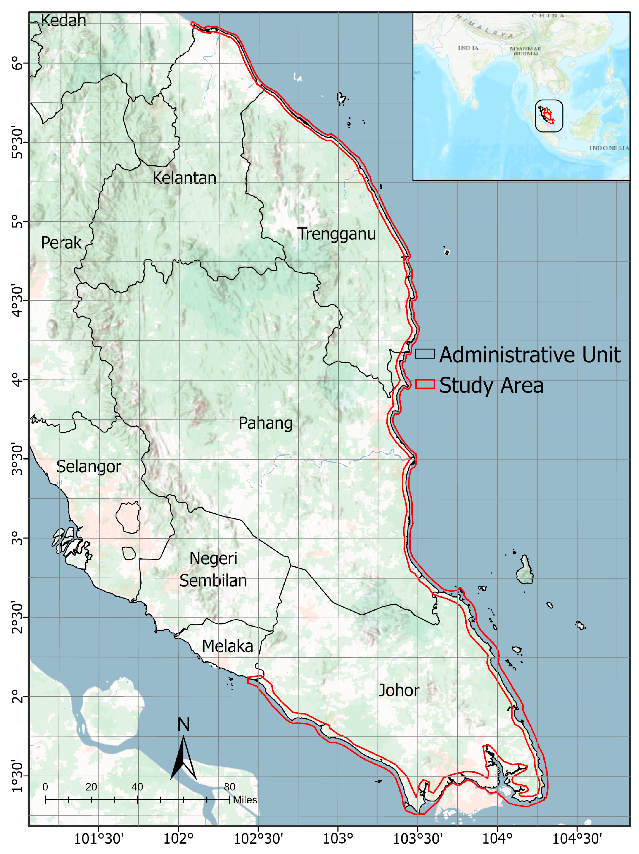
Figure 1. Location map of selected coastal areas along the coast of Malaysian Peninsula.
Remotesensing 17 03334 g001
Figure 2. A comprehensive methodological framework used in this study by integrating Landsat time-series datasets (1990–2024), deep learning modeling, and shoreline change analysis.
Remotesensing 17 03334 g002
Figure 3. U-Net architecture for Land/Sea segmentation of Landsat image. Source: [50]. The figure illustrates the network architecture, where the dark brown triangles represent convolution operations (3 × 3), the green triangles indicate convolution operations (1 × 1), and the yellow blocks represent the up-sampling operations (2 × 2). The arrows depict the flow of data through the network layers, from the input Landsat image with six bands (left) to the output Land/Sea segmented image (right).
Remotesensing 17 03334 g003
Figure 4. DeepLabV3+ architecture for Land/Sea Segmentation of Landsat Images. Source: [50,53]. The figure illustrates the encoder-decoder structure, where the blue region represents the encoder with various convolution operations: 1 × 1 convolution (purple), 3 × 3 convolutions with different dilation rates (orange, pink, and beige), and image pooling. The arrows in the encoder section depict the flow of data through these layers. The red region represents the decoder, with low-level features being upsampled by a factor of 4, followed by 1 × 1 convolution and concatenation. The arrows in the decoder section indicate the progression of features from the encoder to the final upsampled prediction output. The green and pink blocks show the upsampling operations and concatenation process respectively. The final output is a Land/Sea segmentation prediction, shown on the right side.
Remotesensing 17 03334 g004
Figure 5. Training validation loss curves. (a) U-Net model performance, (b) DeepLabV3+ model performance.
Remotesensing 17 03334 g005
Figure 6. Tested performance metrics of models on the 2018 Landsat image.
Remotesensing 17 03334 g006
Figure 7. Detailed visualization of the segmentation results of both models on the 2018 Landsat image. The color boxes around the segmented regions represent areas of interest: red indicates the, water and gray represents segmented land. The yellow boxes highlight the areas where the segmentation performance was evaluated. It is evident from the comparison that the U-Net model provides more accurate segmentation of land and sea areas, particularly along the coastline, as compared to DeepLabV3+.
Remotesensing 17 03334 g007
Figure 8. Comparative analysis of U-Net and DeepLabV3+ segmentation performance on others selected regions. Similar to Figure 7, the results confirm that U-Net provides more accurate segmentation of land and sea regions, particularly along the coastline, in comparison to DeepLabV3+.
Remotesensing 17 03334 g008
Figure 9. Spatial distribution of shoreline change analysis in Kelantan state: LRR results.
Remotesensing 17 03334 g009
Figure 10. Spatial distribution of shoreline change analysis in Kelantan state: NSM results.
Remotesensing 17 03334 g010
Figure 11. Spatial distribution of shoreline change analysis in Trengganu state: LRR results.
Remotesensing 17 03334 g011
Figure 12. Spatial distribution of shoreline change analysis in Trengganu state: NSM results.
Remotesensing 17 03334 g012
Figure 13. Spatial distribution of shoreline change analysis in Pahang state: LRR results.
Remotesensing 17 03334 g013
Figure 14. Spatial distribution of shoreline change analysis in Pahang state: NSM results.
Remotesensing 17 03334 g014
Figure 15. Spatial distribution of shoreline change analysis in Johor state: LRR results.
Remotesensing 17 03334 g015
Figure 16. Spatial distribution of shoreline change analysis in Johor state: NSM results.
Remotesensing 17 03334 g016
Table 1. Details of Landsat data acquisitions for shoreline analysis.
YearSensorProduct LevelBands UsedSource/PlatformHandling ApproachApplication
1990, 1993, 1998Landsat 5 TMLevel 2Blue–SWIRGoogle Earth EngineAnnual composite, cloud-freeShoreline extraction
2002, 2008Landsat 7 ETM+Level 2Blue–SWIRGoogle Earth EngineAnnual composite, cloud-freeShoreline extraction
2014Landsat 8 OLILevel 2Blue–SWIRGoogle Earth EngineAnnual composite, cloud-freeShoreline extraction
2018Landsat 8 OLILevel 2Blue–SWIRGoogle Earth EngineAnnual composite, cloud-freeModel testing
2024Landsat 9 OLILevel 2Blue–SWIRGoogle Earth EngineAnnual composite, cloud-freeModel training/development
Table 2. Data augmentation steps applied during training.
AugmentationParameter RangeDescription
Random Rotation±15°Simulates small orientation changes without distorting shoreline geometry
Horizontal Flipp = 0.5Handles coastline direction variability; common in segmentation tasks
Vertical Flipp = 0.5Adds invariance to shoreline orientation and acquisition geometry
Brightness AdjustmentFactor 0.8–1.2Accounts for seasonal illumination and atmospheric variability in Landsat composites
Table 3. Experimental configuration for model training.
ComponentSettingJustification
Input Tile Size512 × 512 pixelsBalances computational efficiency with sufficient contextual information [27,33]
Loss FunctionBinary Cross-EntropyStable for balanced binary segmentation
Batch Size8Fits GPU memory while maintaining gradient stability.
Epochs20Sufficient for convergence under augmentation
OptimizerAdamAdaptive learning rate; widely adopted for segmentation tasks
Initial Learning Rate1 × 10−4Common default for Adam in semantic segmentation; stable convergence.
LR ScheduleReduceLROnPlateau (factor = 0.5; patience = 3; min LR = 1 × 10⁻⁵)Prevents stagnation; accelerates convergence when validation loss plateaus.
Early StoppingPatience = 5 (monitor validation loss)Stops training when no improvement; reduces overfitting risk
CheckpointingSave best weightsEnsures reproducibility and best generalization
Validation Split20% of training datasetStandard practice for moderate datasets to monitor generalization.
Table 4. The yielded positional uncertainties for 1990–2024 shorelines using a conservative error-budget approach.
YearGeoreferencing Error (Eg) (m)Pixel Error (Ep) (m)Tidal Error (Etide) (m)Total Uncertainty (U) (m)
19905015100112.81
19935015100112.81
19985015100112.81
20025015100112.81
20085015100112.81
20141215100101.83
20181215100101.83
20241215100101.83
Table 5. Training performance metrics of U-Net and DeepLabV3+ models on 2024 Landsat image.
ModelClassPrecisionRecallF1 Score
U-NetLand0.99830.99770.9979
Water0.99870.99910.9989
DeepLabV3+Land0.99730.99720.9973
Water0.99880.99880.9988
Table 6. Summary of DSAS metrics statistics for each of the studied states of Malaysia.
Descriptive StatisticsKelantanTerengganuPahangJohorTotal
Transect ID range1–731732–31663167–52105211–10,6011–10,601
Total no. of Transects73124352044539110,601
Mean Shoreline Change Envelope (SCE)256.460.1143.3103.4111.7
Maximum Shoreline Change Envelope (SCE)2034.21197.2206119262061
Minimum Shoreline Change Envelope (SCE)00.4500.90
Percentage of Transects exhibiting erosion (LRR)30.1133320.521.8
Percentage of Transects exhibiting accretion (LRR)36.9432384138.1
Percentage of stable transects (LRR)32.96552938.540.1
Maximum Erosion (NSM based) (m)−1885.4−364−1658.2−341.4−1885.4
Mean Erosion (NSM based) (m)−78−8.3−41.1−17−23.9
Maximum Accretion (NSM based) (m)1628.511832028.119172028.1
Mean Accretion (NSM based) (m)953162.866.459
Percentage of Transects exhibiting erosion (NSM)32.114.13420.722.5
Percentage of Transects exhibiting accretion (NSM)36.733.8444441.1
Percentage of stable transects (NSM)31.252.12235.336.4
Mean Erosion rate (m/year)−2.9−0.25−1.24−0.52−0.76
Mean Accretion rate (m/year)2.630.981.61.921.7
Disclaimer/Publisher’s Note: The statements, opinions and data contained in all publications are solely those of the individual author(s) and contributor(s) and not of MDPI and/or the editor(s). MDPI and/or the editor(s) disclaim responsibility for any injury to people or property resulting from any ideas, methods, instructions or products referred to in the content.