RPC Correction Coefficient Extrapolation for KOMPSAT-3A Imagery in Inaccessible Regions

Highlights

What are the main findings?

• This study proposes a transport-based RPC correction learned on a small head subset, extrapolating downstream while preserving geometry and yielding <3-pixel tails in two of three strips.
• This study models pushbroom error extrapolation by leveraging satellite orbital parameters and terrain characteristics to transport head-of-strip corrections downstream.

What is the implication of the main finding?

• This study provides a practical alternative to strip-wide block adjustment for control-denied or resource-limited settings, operating in image space and tolerating missing segments or ties.
• This study offers a transferable framework for sub-meter platforms; under stronger dynamics, broader calibration and optional higher-order terms further stabilize transport.

Abstract

High-resolution pushbroom satellites routinely acquire multi-tenskilometer-scale strips whose vendors’ rational polynomial coefficients (RPCs) exhibit systematic, direction-dependent biases that accumulate downstream when ground control is sparse. This study presents a physically interpretable stripwise extrapolation framework that predicts along- and across-track RPC correlation coefficients for inaccessible segments from an upstream calibration subset. Terrain-independent RPCs were regenerated and residual image-space errors were modeled with weighted least squares using elapsed time, off-nadir evolution, and morphometric descriptors of the target terrain. Gaussian kernel weights favor calibration scenes with a Jarque–Bera-indexed relief similar to the target. When applied to three KOMPSAT-3A panchromatic strips, the approach preserves native scene geometry while transporting calibrated coefficients downstream, reducing positional errors in two strips to <2.8 pixels (~2.0 m at 0.710 m Ground Sample Distance, GSD). The first strip with a stronger attitude drift retains 4.589 pixel along-track errors, indicating the need for wider predictor coverage under aggressive maneuvers. The results clarify the directional error structure with a near-constant across-track bias and low-frequency along-track drift and show that a compact predictor set can stabilize extrapolation without full-block adjustment or dense tie networks. This provides a GCP-efficient alternative to full-block adjustment and enables accurate georeferencing in controlled environments.

1. Introduction

1.1. Overview

High-resolution optical satellite imaging has become indispensable in many geographic domains, including environmental monitoring, urban planning, disaster management, and precision agriculture. These satellites provide submeter resolution in visible and near-infrared spectral bands, enabling thorough and rapid investigations of a variety of surface phenomena, from land use changes to urban growth patterns [1,2,3]. However, vendors’ rational polynomial coefficients (RPCs) frequently have systematic geometric inaccuracies that reduce their spot-positioning accuracy, hindering their use in high-precision topographic mapping applications [4]. Inaccurate orbit ephemeris data; minute changes in satellite attitude, such as roll, pitch, and yaw; residual sensor distortions that impact internal sensor calibration; and stray light effects resulting from unintended optical scattering within the sensor system are some of the causes of these problems [5,6,7,8,9]. If systematic errors and uncalibrated parameters are not corrected, they may cause cumulative positioning errors that can reach tens of meters across a long satellite image strip. Although such errors may appear small in certain contexts, they can substantially reduce the accuracy of derived data, such as digital elevation models (DEMs) and orthoimages, particularly in applications requiring high precision, such as flood modeling or critical infrastructure monitoring [10,11,12,13].

Traditional approaches for correcting RPC biases rely on the Ground Control Points (GCPs). These points can generate correction models or adjust satellite images globally [14,15,16]. However, collecting GCPs can be difficult, or even impossible [17]. Consequently, large sections of satellite image strips may remain uncorrected, reducing their reliability for detailed analysis. This is particularly problematic for high-precision geospatial tasks that cover inaccessible areas.

Using the internal consistency of single-orbit image strips is a viable alternative. Parameters such as the camera angle, sensor stability, and satellite speed usually do not change during a single satellite pass. These adjustments could be successfully applied to later sections of the same strip if the RPC biases could be precisely determined using GCPs at the beginning of the strip. According to preliminary studies on block adjustments, combining tie points with a limited number of GCPs can assist in stabilizing the orientation across adjacent images and minimize the requirement for intensive ground control [18]. However, the systematic exploration of this approach, specifically for single-strip imagery, is still limited and requires further study.

The proposed approach has notable advantageous. First, as direct georeferencing is only required for a limited number of scenes, it substantially reduces the need for large ground-based data collection. Second, it facilitates high-precision mapping in inaccessible or hazardous areas without compromising the positional accuracy. Third, this method provides a way to correct gradual geometric distortions that accumulate along the orbital path, particularly when imaging various types of terrain.

This study investigated whether it is possible to extrapolate RPC correction coefficients to later segments using a small number of GCPs at the start of a satellite image strip. To improve the effectiveness and geographic reach of photogrammetric workflows, this study assessed whether a single correction model can sustain accuracy across long distances. If successful, this method might significantly increase the usefulness of high-resolution strip photography in practice, which would help national mapping organizations, the defense industry, and scientific initiatives working on difficult terrains or with political constraints [19].

The proposed approach uses physically interpretable orbital and terrain parameters, which are different from existing approaches, such as affine transformations that require extensive ground calibration or spline interpolation-based block adjustments that rely heavily on dense tie-point networks across overlapping images. The proposed approach ensures scalability, computational simplicity, and adaptability across a variety of operational settings by efficiently predicting the RPC correction coefficients with minimal ground control.

1.2. Literature Review

Hong et al. [20] investigated ways in which insufficient sensor calibration and orbit and attitude errors can induce systematic biases that, if left uncorrected, can degrade the geo-positioning of high-resolution satellite images by several meters (≈0.002° at QuickBird’s 450 km altitude), sometimes even by tens of meters (≈0.003°). Identical angular biases cause proportionally different ground offsets depending on the satellite orbital altitude, thereby enabling generalization to any imaging platform. By creating discrepancies between the nominal picture coordinates and actual ground placements, these biases jeopardize precision-dependent applications, including environmental surveillance, critical infrastructure monitoring, and accurate urban mapping. This study investigated several bias compensation techniques, including simple translational corrections in orbital or image spaces and polynomial refinements of various orders. The results demonstrate that both Rational Functional Models (RFMs) and Rigorous Sensor Models (RSMs) can attain subpixel or almost subpixel precision if sufficient GCPs are strategically positioned throughout the image. Crucially, when the systematic errors were removed, neither model type outperformed the others. As a result, the choice of modeling strategy is often influenced by elements such as the degree of computational resources, availability of metadata, and level of user community expertise.

Xiong and Zhang [21] discussed a situation in which the RPCs may have substantial ephemeris and attitude problems that surpass the ability of more straightforward shift-based techniques to rectify them. Larger orbital uncertainties result from satellites frequently performing partial calibrations if they are modest missions or projects with limited funding. In these situations, the authors suggested building a pseudo-rigid sensor model by estimating the sensor orientation from the nominal RPC. This model was subsequently improved using carefully selected GCPs. Physically demanding camera characteristics are no longer required when the modified orientation is finalized and reincorporated into a new or updated RPC set. End users who require precise geopositioning for tasks such as land cover mapping, feature extraction, or 3D city modeling but do not have access to proprietary ephemeris and camera data would find this practical method useful. When GCPs are abundant and appropriately distributed, tests using both synthetic and actual data demonstrate how well the method bridges the gap between physically grounded sensor models and purely polynomial solutions, thereby producing subpixel precision.

Topan et al. [22] emphasized the interplay between refined sensor models and DEMs for producing orthoimages. Even if the sensor orientation is refined to subpixel levels, a DEM that diverges from real terrain heights can project vertical errors into horizontal offsets, particularly in mountainous or hilly areas. The authors demonstrated that a vertical mismatch of a few meters can result in multi-pixel horizontal errors, negating the advantages of polynomial bias corrections using strategies such as the figure condition method. Therefore, when precise orthoimages are needed, practitioners should invest in high-quality elevation data because the synergy between accurate DEM data and well-bias-corrected RPC parameters is essential for achieving constant sub-pixel accuracy in challenging terrains.

Shen et al. [4] investigated how thin-plate spline interpolation handled local and global aberrations in a single continuous framework beyond polynomial patches. Splines distribute the influence of each GCP over a large area and are excellent at adjusting to gradually fluctuating errors caused by small shifts in satellite orientation, ephemeris drift, or local sensor misalignments. Although TPS can outperform classic polynomials in capturing subtle distortions, the authors noted that the computational overhead of the method increases with the number of GCPs and demands careful selection of smoothing parameters to avoid overfitting. Nevertheless, for high-resolution satellites covering broad areas, the TPS can deliver significantly reduced residuals if the GCP network is extensive and properly configured.

In Toutin’s study [23], the distortion sources were divided into four categories—platform-related (such as orbit ephemeris), sensor-related (such as lens distortion and scanning geometry), Earth-related (such as curvature and topographic relief), and projection-related (such as map coordinate frames) sources—offering a more comprehensive view of geometric corrections. According to the author, accurate orbital and attitude data are used by rigorous sensor models to calculate picture coordinates from ground locations. However, this connection is approximated by empirical methods, such as polynomial or rational function models, using the ratios of polynomial functions. The author also discussed stereo-based scene reconstruction, multi-image block adjustments, and error propagation, emphasizing that the effectiveness of each technique depends on how well the model complexity, ground data availability, and project accuracy requirements work together. The necessity for sophisticated orientation or correction techniques has grown as sensors have become more accurate, particularly in commercial satellites with submeter resolutions.

This desire for improvement is evident in the study by Li et al. [24], who described a process for satellites burdened with substantial initial offsets or insufficient calibration. Using a network of ground controls, they suggested iteratively fine-tuning the external orientation parameters (roll, pitch, and yaw) and even the partial internal orientation before regenerating or re-fitting the RPCs. The virtual GCPs are stretched over the image once the geometry is stabilized, thereby densifying the control of the final polynomial solution. A vendor-provided RPC with flaws was replaced with an updated set of coefficients that can provide near-meter or higher planimetric precision. Using this method, data from smaller satellites, which may not have reliable on-orbit calibration, can be recovered, making them competitive candidates for jobs that are traditionally performed by fully rigorous missions.

Titarov [25] examined the geometric capability of Cartosat-1 (IRS P5) stereo imagery for DEM generation and orthoimage production. The author evaluates various orientation methods, including bias and drift adjustments, applied to the RPC model. The results demonstrate that the sub-pixel orientation accuracy for a single stereo pair can be attained using four well-distributed ground control points. When extended to a block of overlapping stereo pairs, the workload of the GCPs can be reduced by using tie points in the overlapping areas. The empirical results indicated that DEMs derived from flat terrain exhibited an RMSE of approximately 2 m, whereas those derived from mountainous areas increase to approximately 7 m. Nonetheless, the orthorectified imagery meets the accuracy requirements for 1:10,000-scale mapping. Thus, this study underscores Cartosat-1’s capacity for large-scale photogrammetric tasks, noting that simple bias-and-drift corrections of the RPC model yield reliable results without necessitating more complex rigorous sensor models.

Liu et al. [26] examined DEM generation using WorldView-2 stereo images over a plateau with significant topographic relief by comparing along-track pairs with multi-orbit combinations captured at different times. The authors used a reference DEM and in situ ground control points to evaluate the horizontal and vertical accuracies using both rigorous sensor models and rational function models. The findings show that multi-orbital stereo data can still meet the 1:5000 mapping criteria if appropriately corrected; however, along-track pairs generally produce a somewhat higher precision owing to a more constant viewing geometry. This study emphasizes the need for appropriate bias compensation because significant terrain changes magnify disparities from ephemeris or interior calibration problems. The findings indicate that although the DEM accuracy decreases with increasing off-nadir angles, it is still suitable for the majority of engineering or cartographic applications, particularly when strong ground control is provided.

Finally, Fraser et al. [27] provided empirical evidence indicating that imagery initially exhibiting positional offsets of several tens of meters, such as the Ikonos Geo imagery, can achieve submeter horizontal accuracy. Applying appropriate bias adjustments, along with a small number of GCPs, allows for this refinement. To produce 3D urban models that are accurate to within approximately a meter, the authors described a pipeline that comprises stereo matching, feature extraction, and building outline generation. They pointed out that automatic matching is still hampered by shadows, reflective surfaces, and intricate urban patterns; however, these problems are more related to computer vision algorithms than to basic sensor geometry. It is now possible to create city-scale 3D reconstructions from reasonably accessible commercial photographs by methodically eliminating orientation biases, enabling the detection of building corners, rooftop edges, and street alignments with greater accuracy.

In addition, various studies have pursued the calibration of physical sensor models and associated error parameters to generate accurate Rational Polynomial Coefficients. Seo et al. [28] conducted a geometric calibration of a high-resolution camera on the KOMPSAT-3A satellite, correcting both internal and external parameters, including boresight alignment, CCD sensor alignment, and focal length, directly in orbit. After calibration using imagery from multiple test sites over two months, they evaluated the geolocation accuracy across hundreds of global points without ground control points, and validated the planar positioning accuracy using bundle adjustment with ground control points. The calibration successfully eliminated systematic errors in the sensor model, significantly enhancing the absolute geolocation accuracy of the satellite imagery. Pan et al. [29] performed a self-calibration dense-bundle adjustment on multiview basic imagery from the WorldView-3 satellite. By refining errors in both exterior orientation parameters, such as attitude jitter, and interior orientation parameters based on an RSM, they achieved substantial improvements in the accuracy of ground coordinate determination. Eftekhari et al. [30] introduced methods to generate and refine RPCs for TerraSAR-X Synthetic Aperture Radar (SAR) imagery. Initially, the RPCs derived from the physical radar sensor model exhibited positional biases of several pixels owing to orbit errors. To mitigate these errors, they recalibrated the timing and sampling parameters, including the pulse repetition frequency, using a minimal number of GCPs and applied an affine correction model in the image space. Schneider et al. [31] compared hyperspectral data processing workflows for airborne (HySpex) and spaceborne (EnMAP) sensors, emphasizing the critical importance of calibration, stray-light correction, and RPC model generation. This study particularly underscores the importance of addressing stray light effects to improve the accuracy of RPCs across different sensor platforms.

In conclusion, previous studies collectively highlight that ephemeris and attitude uncertainties, incomplete sensor calibration, terrain complexity, ground control distribution, DEM fidelity, and polynomial modeling all critically affect RPC correction. Even minor orbital misalignments can result in offsets of tens of meters, particularly when traveling across rough terrain, where errors in the DEM spread into horizontal inaccuracy. Strategically placed GCPs reduce local biases, whereas limited coverage encourages overfitting and residual distortions. Although spline-based techniques and high-order polynomials can handle nonuniform error patterns, they require careful parameter tweaking and a sufficiently dense GCP network. Finally, the availability of sensor metadata, mission stability, and the required degree of mapping accuracy determine whether to use straightforward bias-and-drift corrections or complex reorientation techniques. For large-scale applications, such as infrastructure planning and urban modeling, practitioners can attain sub-pixel results by striking a balance between these parameters, especially in high-relief locations.

Practical extrapolation of correction coefficients across large inaccessible regions using minimal ground calibration data remains a critical research gap, although previous studies have successfully addressed RPC biases using various polynomial-based and spline interpolation methodologies. Current approaches rely frequently on dense tie-point configurations or evenly spaced ground control points, which are rarely achieved in isolated, difficult-to-reach, or constrained settings. Furthermore, the rigorous data requirements of affine and traditional block modifications, along with the computational load and overfitting vulnerability of spline-based approaches, severely limit the operational flexibility.

Expanding on previous discoveries, the current study presents a new extrapolation-based RPC correction technique created specifically for pushbroom satellite images taken in areas with little to no ground access. By predicting the RPC correction coefficients from an upstream calibration subset using physically interpretable orbital and terrain parameters, the proposed approach is unique because it significantly reduces the need for extensive GCP networks. This study offers a useful and affordable substitute for traditional block adjustment techniques by proving that linear extrapolation models can capture longitudinal biases with limited data. This method improves geographic accuracy and analytical dependability across a range of remote sensing applications by expanding operational applicability in controlled denied contexts and providing a solid framework that is easily transferable to additional submeter optical satellite platforms.

1.3. Research Objectives

The purpose of this study is to identify and analyze the key elements influencing the estimation of RPC correction coefficients in a controlled single-strip imaging scenario, with special emphasis on places with limited ground access. This study methodically investigated the relative effects of topographic complexity, viewing geometry, and temporal variation on the stability and transferability of the RPC correction parameters in this limited setting. This process uses a small number of ground control points obtained from the accessible section of the strip to establish a baseline correction model that is subsequently spread downstream to regions without direct control information. Through quantitative modeling and empirical validation, this study sought to enhance the robustness and efficiency of RPC-based georeferencing workflows, ultimately enabling accurate mapping and terrain reconstruction in operationally inaccessible regions. In contrast to conventional on-orbit sensor calibration methods that directly refine the internal and external geometric sensor parameters based on telemetry data, such as star trackers or inertial navigation logs, the proposed approach performs corrections at the image-coordinate level using a simplified linear extrapolation model. This method requires only a limited number of GCPs from the initial images without dependence on detailed sensor configuration knowledge or proprietary telemetry data, thus providing improved operational flexibility and applicability in resource-constrained or restricted access scenarios typical of civilian KOMPSAT-3A applications. Beyond enhancing operational flexibility, this study establishes a transferable framework that bridges physical imaging geometry with empirical error modeling, thereby reducing the dependency on dense GCP networks and enabling consistent submeter georeferencing across diverse orbital conditions and terrain complexities. The main contributions of this research are as follows:

• Strip segment RPC correction coefficient extrapolation that preserves native scene geometry and reduces GCP dependence. The method calibrates on a small upstream subset and transports correction coefficients to downstream segments, providing a practical alternative to strip-wide block adjustment in control-denied or resource-constrained settings.
• Physically grounded predictor design with morphometry-aware similarity weighting for stable transport. The model uses elapsed time, off-nadir change, and terrain morphometry, and implements a Jarque–Bera- or σ_DEM-guided similarity weight in a weighted least square fit to emphasize calibration scenes that resemble the target segment.
• Operational validation on KOMPSAT-3A long strips with effective along-track drift control. Experiments on three strips confirm the directional error structure and show sub-3-pixel downstream errors in two strips, clarifying when transport-based extrapolation outperforms strip-replacement strategies.

2. Methodology

2.1. Overview

Section 2.1 Overview provides a brief description of the structure of the Methodology Section and explains the corresponding flowchart. The first part of the Methodology Section presents the sensor and orbit physical modeling of KOMPSAT-3A (Section 2.2 and Section 2.3). Figure 1 shows the overall flowchart of the study. On the left-hand side of the flowchart, the RPCs and their corresponding correction coefficients were computed using Advanced Spaceborne Thermal Emission and Reflection Radiometer (ASTER) Global Digital Elevation Model Version 2 (GDEM V2) V2, KOMPSAT-3A strip images, and the associated metadata. The detailed calculation procedures are described in Section 3.2.1 and Section 3.2.2. The acquisition process for the GCPs and checkpoints (CKPs) using a digital map, high-resolution DEM, and aerial orthophotos is outlined on the right-hand side. The core of the proposed approach is elaborated in Section 2.5, where the extrapolation-based correction framework is described in detail. The procedures for GCP acquisition are comprehensively described in Section 3.2 and Section 3.3. Finally, the bottom section of the flowchart explains the prediction of the RPC correction coefficients for the latter portions of each strip based on the coefficients derived from images at the beginning of the strip and the subsequent comparison of these predicted values with the actual correction coefficients. The results of this study and their corresponding discussions are presented in Section 4 and Section 5, respectively.

2.2. KOMPSAT-3A Sensor

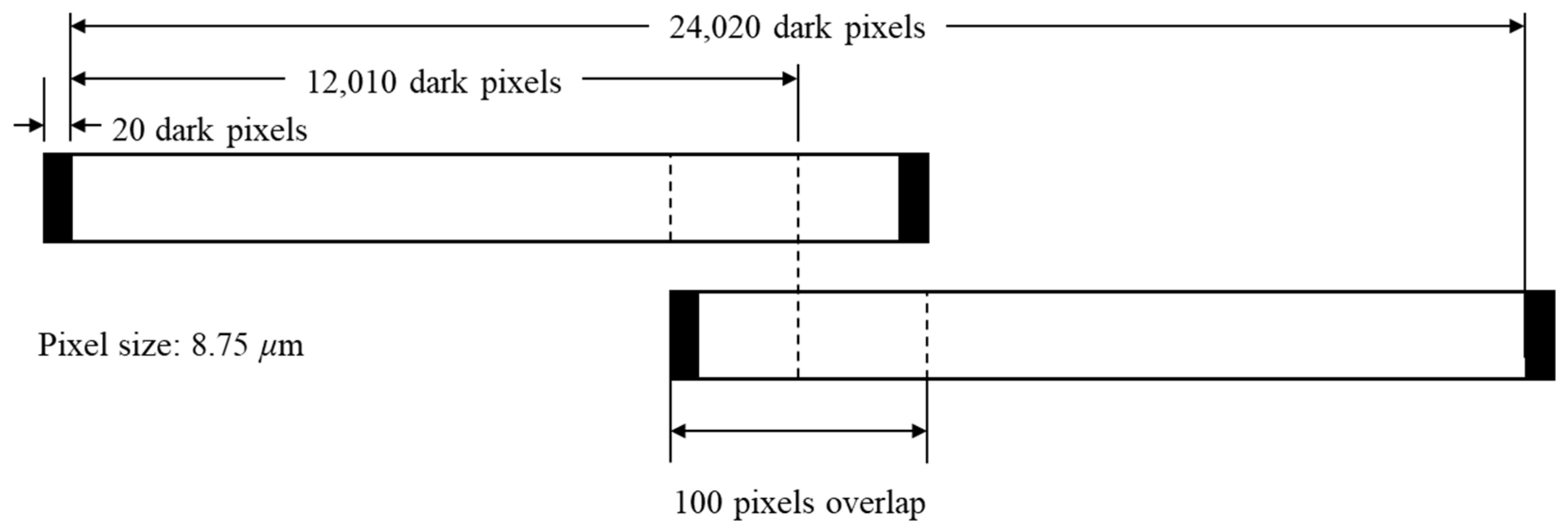
The KOMPSAT-3A satellite, launched in 2015, carries the Advanced Earth Imaging Sensor System A (AEISS-A), which is a high-resolution Earth observation camera that shares structural similarities with the earlier AEISS sensor on KOMPSAT-3 [28]. The AEISS-A sensor simultaneously captures imagery in the panchromatic (PAN) and multispectral (MS) bands and features an additional Mid-Wavelength Infrared (MWIR) thermal imaging sensor, known as the Infrared Imaging Sensor (IIS), enhancing its nighttime and thermal observation capabilities [32]. Specifically, the PAN channel of the AEISS-A is composed of two linear time-delay integration (TDI) CCD arrays, each approximately 12,080 pixels wide, combined with a total swath width of approximately 24,020 pixels [28,33,34]. TDI technology, incorporating up to 64 integration stages, ensures a sufficient signal-to-noise ratio (SNR) even at very high spatial resolutions [35]. The MS channel also employs TDI functionality, with each spectral band comprising linear CCD arrays that are approximately 6000 pixels wide. The pixel pitch was approximately 8.75 µm for the PAN band and 35 m for the MS bands, maintaining a ratio of 1:4, which is consistent with their respective ground sampling distances.

The designed orbital altitude of KOMPSAT-3A is approximately 528 km, resulting in ground sample distances (GSD) of approximately 0.55 m for PAN imagery and 2.2 m for MS imagery [28,32]. At the nadir viewing geometry, both the PAN and MS bands achieved an image swath width ranging between 12 and 16 km. The optical system utilizes a Korsch-type telescope with a 0.8 m aperture and an f/12 focal ratio, enabling the simultaneous and co-registered acquisition of PAN and MS data. The radiometric resolution of the sensor was 14 bits with an SNR exceeding 100 for both PAN and MS imagery [32].

Owing to the configuration of multiple linear CCD arrays, the raw imagery acquired by the AEISS-A sensor initially consisted of multiple segmented scenes. For PAN imagery, these segments require precise geometric stitching and merging of images captured from two adjacent CCD arrays to form a seamless final image product [33]. Figure 2 shows the configuration of the AEISS-A panchromatic CCD sensor onboard KOMPSAT-3A [28,34].

KOMPSAT-3 and KOMPSAT-3A underwent meticulous pre- and post-launch geometric calibration procedures utilizing overlapping areas (several tens of pixels wide) between the CCD segments to achieve accurate internal alignment. After the completion of this internal geometric correction and stitching process, users receive fully integrated PAN imagery, enabling further geospatial analyses and applications, including the accurate regeneration of RPCs.

2.3. KOMPSAT-3A Sensor Modeling

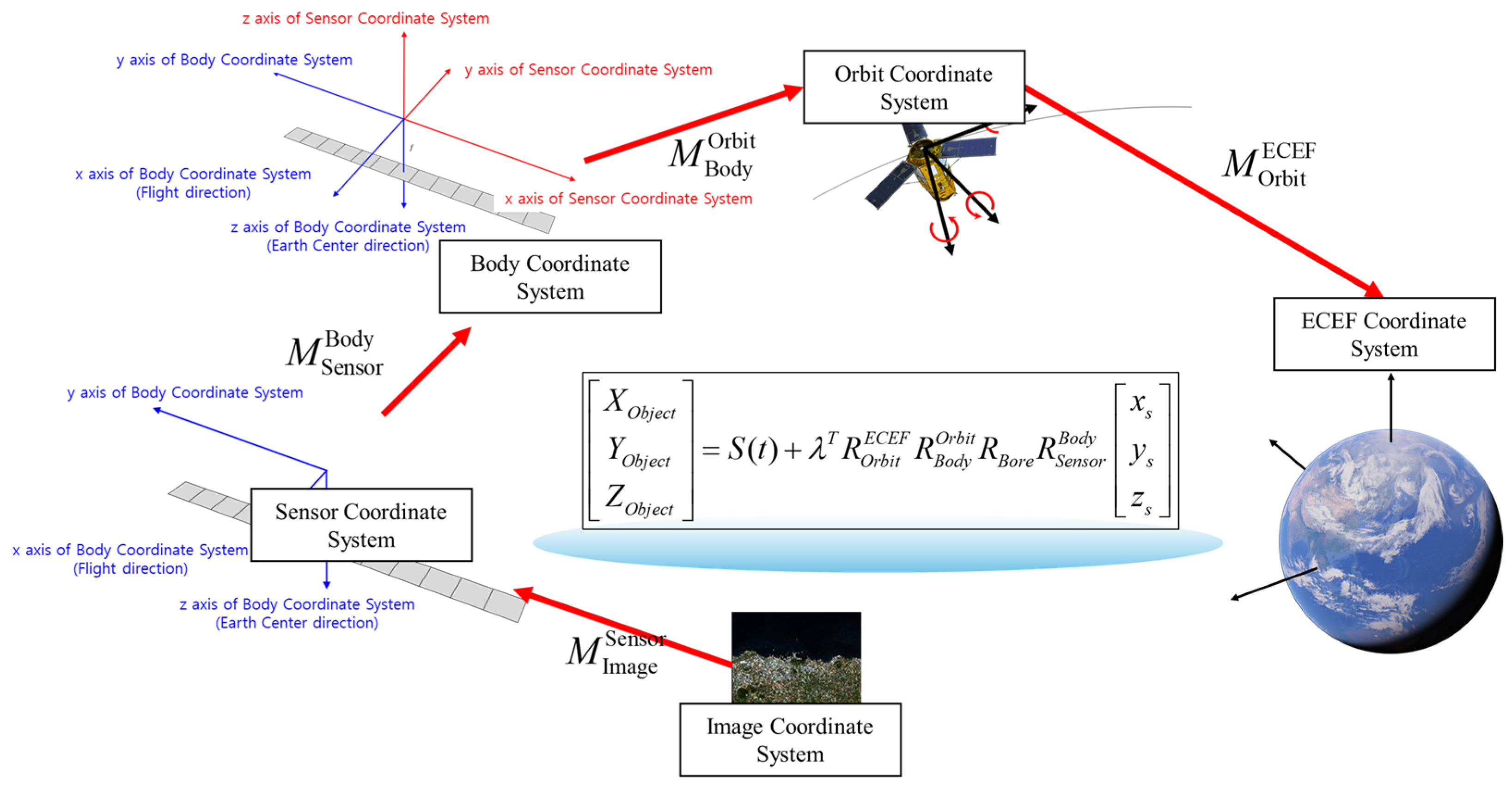
Rigorous physical sensor modeling for the KOMPSAT-3A high-resolution optical satellite requires the definition and interrelation of five distinct coordinate systems. These frames of reference include the Image Coordinate System, intrinsic to the captured digital image; the Sensor Coordinate System, aligned with the focal plane array and optical axis; the Body Coordinate System, fixed to the satellite platform structure; the Orbital Coordinate System, describing the satellite’s motion relative to its orbit; and the Earth-centered Earth-fixed (ECEF) coordinate system, a geodetic reference frame co-rotating with the Earth. Establishing precise definitions for each system is a prerequisite for accurate geospatial positioning. The core of the georeferencing process involves transforming the image point coordinates from the image coordinate system into their corresponding ground coordinates in the ECEF frame. This transformation is achieved through a cascaded series of rotations and translations, mathematically represented by rotation matrices. Following photogrammetric notation, $M_A^B$ denotes the 3 × 3 rotation matrix that transforms the vector coordinates from frame A to frame B, where $R_B^A=M_A^B$. Figure 3 shows the coordinate transformation process of KOMPSAT-3A using a physical sensor model [34].

Finally, the collinearity equation specific to KOMPSAT-3A is expressed as given in Equation (1).

$$\left[\begin{array}{c}{X}_{Object}\\ Y_{Object}\\ Z_{Object}\end{array}\right]=S\left(t\right)+\lambda ·{\mathrm{M}}_{\mathrm{O}\mathrm{r}\mathrm{b}\mathrm{i}\mathrm{t}}^{\mathrm{E}\mathrm{C}\mathrm{E}\mathrm{F}}·{\mathrm{M}}_{\mathrm{B}\mathrm{o}\mathrm{d}\mathrm{y}}^{\mathrm{O}\mathrm{r}\mathrm{b}\mathrm{i}\mathrm{t}}·{\mathrm{M}}_{\mathrm{B}\mathrm{o}\mathrm{r}\mathrm{e}}·{\mathrm{M}}_{\mathrm{S}\mathrm{e}\mathrm{n}\mathrm{s}\mathrm{o}\mathrm{r}}^{\mathrm{B}\mathrm{o}\mathrm{d}\mathrm{y}}·\left[\begin{array}{c}{x}_s\\ y_s\\ z_s\end{array}\right]$$

(1)

where $\lambda$: scale coefficient, ${\mathrm{M}}_{\mathrm{B}\mathrm{o}\mathrm{r}\mathrm{e}}$: Boresight Rotation Matrix, $S\left(t\right)$: Satellite position at time t, ${\left[\begin{array}{ccc}{x}_s& y_s& z_s\end{array}\right]}^T$: sensor coordinates.

Accurate determination of a satellite’s Exterior Orientation Parameters (EOPs), specifically, its position (X, Y, Z in ECEF) and attitude (roll, pitch, and yaw), is critical. Because KOMPSAT-3A operates as a pushbroom scanner, these EOPs must be known for each acquired scan line. High-frequency EOP information is typically obtained by interpolating the precise ephemeris (position) and attitude data of a satellite, which are provided as discrete time-tagged measurements. In this study, the temporal variation in the EOPs across the imaging interval was modeled using a second-order polynomial function. The proposed approach allows for a continuous representation of the satellite trajectory and orientation based on discrete ephemeris points.

Ultimately, the geometric relationship linking the satellite’s perspective center (projection origin), a point object on the Earth’s surface, and its corresponding image point is governed by the collinearity condition. This fundamental principle of photogrammetry expressed within the ECEF coordinate system mathematically enforces the idea that these three points lie along a single straight line representing the observation vector or line-of-sight from the sensor to the ground. Accurate modeling of these coordinate systems, transformations, and the application of the collinearity condition are essential for deriving precise ground coordinates from KOMPSAT-3A imagery.

2.4. RFM

RFM establishes a mathematical relationship between the ground coordinates and the corresponding image coordinates, typically employing a third-order polynomial function. This model facilitates conversion from ground-based latitude, longitude, and altitude coordinates to image coordinates (rows and columns), and vice versa. RPCs have been widely adopted owing to their system-independent nature and capability for real-time computation without requiring detailed knowledge of individual sensor systems [36]. To ensure robust and stable RPC estimations, normalization of both ground and image coordinates within the interval [−1, 1] is necessary. Equations (2) and (3) describe the normalization processes for the image and ground coordinates, respectively.

$$i_n={\displaystyle \frac{i-i_O}{i_s}}, j_n={\displaystyle \frac{j-j_O}{j_s}}$$

(2)

$$X_n={\displaystyle \frac{X-X_O}{X_s}}, Y_n={\displaystyle \frac{Y-Y_O}{Y_s}}, Z_n={\displaystyle \frac{Z-Z_O}{Z_s}}$$

(3)

where $i_n, j_n$ are normalized image coordinates, $i_O, j_O$ are offset parameters, $i_s, j_s$ are the scale parameters of the image coordinates. $X_n,Y_n,Z_n$ are the normalized ground coordinates; $X_O,Y_O,Z_O$ are the offset parameters; $X_S,Y_S,Z_S$ are the scale parameters of the ground coordinates.

The normalized ground and image coordinates are defined by the ratio of polynomials, as shown in Equation (4).

$$i_n={\displaystyle \frac{A\left(X_n,Y_n,Z_n\right)}{B\left(X_n,Y_n,Z_n\right)}}, j_n={\displaystyle \frac{C\left(X_n,Y_n,Z_n\right)}{D\left(X_n,Y_n,Z_n\right)}}$$

(4)

where A, B, C, and D are the polynomials of the RFM, and can be expressed by the following Equation (5) in the case of 3rd order polynomials.

$$\begin{gathered} A=\sum _{i=0}^3\sum _{j=0}^i\sum _{k=0}^j{a}_m{X}_n^{i-j}{Y}_n^{j-k}{Z}_n^k, B=\sum _{i=0}^3\sum _{j=0}^i\sum _{k=0}^j{b}_m{X}_n^{i-j}{Y}_n^{j-k}{Z}_n^k \\ C=\sum _{i=0}^3\sum _{j=0}^i\sum _{k=0}^j{c}_m{X}_n^{i-j}{Y}_n^{j-k}{Z}_n^k, D=\sum _{i=0}^3\sum _{j=0}^i\sum _{k=0}^j{d}_m{X}_n^{i-j}{Y}_n^{j-k}{Z}_n^k \\ m={\displaystyle \frac{i\left(i+1\right)\left(i+2\right)}{6}}+j\left(j+1\right)+k, \hspace{1em}{b}_0=d_0=1 \end{gathered}$$

(5)

2.4.1. RPCs Generation

In previous studies, two distinct approaches were employed to estimate RPCs. The first approach is applied when a physical sensor model is unavailable [36,37]. This method requires at least 39 GCPs to determine 78 RPCs, with additional GCPs recommended to ensure redundancy and improve accuracy. The second approach employs a terrain-independent methodology by generating a virtual grid that spans the targeted geographic extent. This method generates a virtual grid covering the target geographic area. Subsequently, each cell within this grid is transformed into satellite image coordinates using the available physical sensor model. The RPC extraction was then accomplished by relating the satellite image coordinates to the corresponding 3D coordinates derived from the virtual grid.

There are two additional application scenarios in the terrain-independent model. The first scenario involved updating or calibrating the parameters within the physical sensor model. The second scenario omits any corrections to the physical sensor parameters by directly utilizing a virtual grid. The virtual grid consists of numerous artificially generated points, providing ample control points, including not only real ground-level coordinates, but also virtual points extending below the ground surface or into the airspace above. Consequently, the virtual-grid method significantly increases the availability and flexibility of GCPs.

A DEM of the target region was acquired to construct the virtual grid (Figure 4a). Based on this DEM, a comprehensive virtual grid was established by defining suitable latitudinal, longitudinal, and altitudinal ranges (Figure 4b). Finally, a virtual satellite image is generated to correlate the 3D virtual grid points with their corresponding satellite image coordinates using the physical sensor model, as illustrated in Figure 4c.

Tao and Hu [37] utilized the Gauss-Markov model (GMM) to determine the RPCs, as shown in Equation (6).

$$\mathrm{P}y=\mathrm{P}\mathrm{A}\xi -e$$

(6)

In this context, $y$ represents the vector of observed values, specifically pixel coordinates derived from the control points; $\xi$ denotes the unknown parameter vector corresponding to the RPCs; $\mathit{e}$ symbolizes the residual vector; $\mathrm{A}$ is the design or Jacobian matrix; and $\mathrm{P}$ refers to the weighting matrix. In the GMM-based approach for estimating RPCs, the diagonal entries of weighting matrix $\mathrm{P}$ are inversely proportional to the denominator term of the RFM equations. The estimation procedure for obtaining the RPC parameters via GMM is shown in Equation (7).

$$\widehat{\xi }={\left({\mathrm{A}}^{\mathrm{T}}\mathrm{P}\mathrm{A}\right)}^{-1}{\mathrm{A}}^{\mathrm{T}}\mathrm{P}y$$

(7)

2.4.2. RPCs Correction Coefficients

The image-correction procedure aims to eliminate the systematic residual errors within the image coordinate space. According to previous research [38], three distinct models are typically applied: image translation, shift-and-drift, and affine transformation. The image translation model addresses systematic offsets using two parameters that represent shifts along the image coordinate axes. The shift-and-drift model extends this correction by incorporating two additional parameters to account for scale differences. These two models are described mathematically by Equations (8) and (9), respectively. Finally, the affine transformation model, defined by Equation (10), further generalizes the correction by allowing both linear shifts and scaling, as well as rotations and shears within the image coordinate system.

$$\left[\begin{array}{c}{i}^{\prime }\\ j^{\prime }\end{array}\right]=\left[\begin{array}{c}i\\ j\end{array}\right]+\left[\begin{array}{c}{O}_i\\ O_j\end{array}\right]$$

(8)

$$\left[\begin{array}{c}{i}^{\prime }\\ j^{\prime }\end{array}\right]=\left[\begin{array}{cc}{S}_i& 0\\ 0& S_j\end{array}\right]\left[\begin{array}{c}i\\ j\end{array}\right]+\left[\begin{array}{c}{O}_i\\ O_j\end{array}\right]$$

(9)

$$\left[\begin{array}{c}{i}^{\prime }\\ j^{\prime }\end{array}\right]=\left[\begin{array}{cc}{R}_1& R_2\\ R_3& R_4\end{array}\right]\left[\begin{array}{c}i\\ j\end{array}\right]+\left[\begin{array}{c}{O}_i\\ O_j\end{array}\right]$$

(10)

Here, i and j denote the original coordinates of an image point obtained from the RPCs; $O_i, O_j$ represent offset parameters; $S_i, S_j$ are scale parameters; $R_1, R_2, R_3, R_4$ refer to individual components of the rotation matrix; and $i^{\prime },j^{\prime }$ indicate the corrected image coordinates.

2.5. Influencing Factors on RPC Correction Coefficients

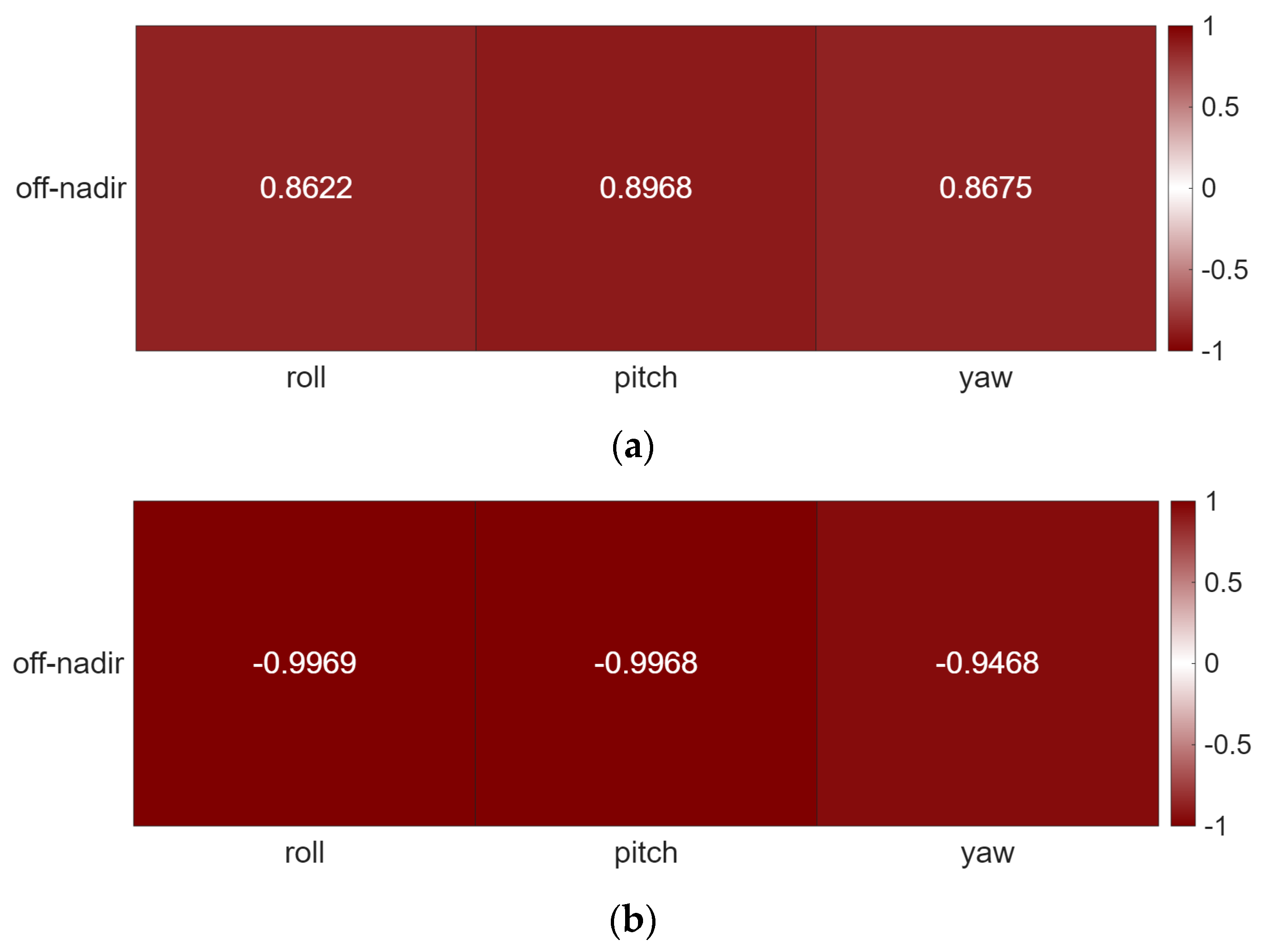
In this study, the critical parameters that effectively represent satellite EOPs and terrain characteristics were identified and utilized to develop an extrapolation model. The parameters chosen to depict satellite EOPs included temporal changes, position variations over time, and velocity fluctuations. These parameters, available from satellite auxiliary files, can generally be modeled using elapsed time (Δt) and indeed show high correlation coefficients with respect to Δt. However, satellite attitude variations tend to be independent of Δt, as attitude angles may be intentionally adjusted at specific times or altered owing to external influences. Attitude parameters include roll, pitch, yaw, and off-nadir angle changes, and these can be simplified to a single parameter, the change in off-nadir angle (Δθ_off-nadir). Figure 5 illustrates the strong correlation between the off-nadir angle and the attitude.

Finally, to represent the terrain characteristics of each target region, the standard deviation of pixel values from the ASTER GDEM data corresponding to the satellite imagery was adopted (σ_DEM). Summarizing, this study proposes an extrapolation model estimating RPC correction coefficients using the parameters Δt, Δθ_off-nadir, and σ_DEM.

After extracting these critical satellite parameters, the relationships between each parameter and the RPC correction coefficients were analyzed individually for each strip. A linear extrapolation model based on the representative orbit parameters was selected because higher-order polynomial models (such as quadratic or cubic models) could potentially cause overfitting. Parameters exhibiting either an absolute correlation coefficient greater than 0.6 or the highest absolute correlation with the RPC correction coefficients were selected to construct the model. Pearson’s correlation coefficients were used to quantify these relationships. Finally, an extrapolation model was established for each strip. In particular, information from the first four images of each strip was used to estimate the model parameters, which were then used to forecast the RPC correction coefficients for the images in the remaining portion of each strip. Equation (11) represents the extrapolation model, where c denotes the along-track direction and r denotes the across-track direction.

$$\begin{gathered} \widehat{c}={\alpha }_{0c}+{\alpha }_c\Delta t+{\beta }_c{\sigma }_{DEM}+{\gamma }_c\Delta {\theta }_{off-nadir}+{\delta }_{c}JB \\ \widehat{r}={\alpha }_{0r}+{\alpha }_r\Delta t+{\beta }_r{\sigma }_{DEM}+{\gamma }_r\Delta {\theta }_{off-nadir}+{\delta }_{r}JB \end{gathered}$$

(11)

The Jarque–Bera (JB) framework combines 3rd- and 4th-moment departures from normality by aggregating the sample skewness S and kurtosis K relative to the Gaussian benchmark $K=3$. In its classical test form, the statistic is $JB={\displaystyle \frac{n}{6}}\left(S^2+{\displaystyle \frac{{\left(K-3\right)}^2}{4}}\right)$ and is asymptotically ${\chi }^2$ with two degrees of freedom under normality, which makes it a compact quantitative measure of asymmetry and tail weight in a distribution. In geospatial applications, higher-order moments are informative regarding local relief structures. Skewness captures asymmetric terrain elements, such as cliff-hollow contrasts, and $K-3$ responds to sharp ridges, scarps, and incised valleys that generate heavy tails in the elevation distribution. Prior DEM studies used the Jarque–Bera diagnostic to evaluate the normality of elevation errors before uncertainty propagation, underscoring the practical value of moment-based characterization when modeling terrain-driven processes.

Guided by these considerations and correlations, this study operationalized a scale-free morphometric predictor.

$$JB=S^2+{\displaystyle \frac{{\left(K-3\right)}^2}{4}}$$

(12)

which removes the sample size term from the classical test and the center kurtosis from the Gaussian reference. This dimensionless index is invariant to the affine rescaling of elevation, directly comparable across scenes and window sizes, and increases monotonically with either greater asymmetry or heavier tails. Therefore, higher-order morphometry was condensed into a single predictor while preserving model parsimony.

The model parameters are estimated using a weighted least-squares framework. In this approach, the weighting strategy was adapted to the morphometric characteristics of the terrain, with the Jarque–Bera index serving as the primary governing metric. The standard deviation of the DEM was employed as a secondary criterion when the Jarque–Bera index was not available. For each extrapolation target, higher weights were assigned to the calibration data whose terrain attributes most closely resembled those of the target scene. To operationalize this strategy, a Gaussian kernel of the form in Equation (13) was employed:

$$w_i=\exp \left(-{\displaystyle \frac{{\left(z_i-z_t\right)}^2}{2h^2}}\right)$$

(13)

where $z_i$ denotes the attribute of the calibration scene i, $z_t$ denotes the attribute of the target scene, and h is set equal to the standard deviation of the calibration attributes. This design ensures that calibration scenes with morphometric characteristics similar to those of the target receive weights approaching unity, whereas dissimilar cases are progressively down-weighted. The final weights were subsequently normalized such that their sum was equals to one, ensuring consistency across extrapolation targets. By emphasizing morphologically comparable regions in the regression process, the method stabilizes the extrapolation of the RPC correction coefficients while maintaining sensitivity to terrain-driven variability. Consequently, the extrapolated coefficients approximate the RPC correction parameters of the satellite images acquired under terrain conditions similar to those of the target scene more closely.

2.6. Summary of the Proposed Extrapolation Module

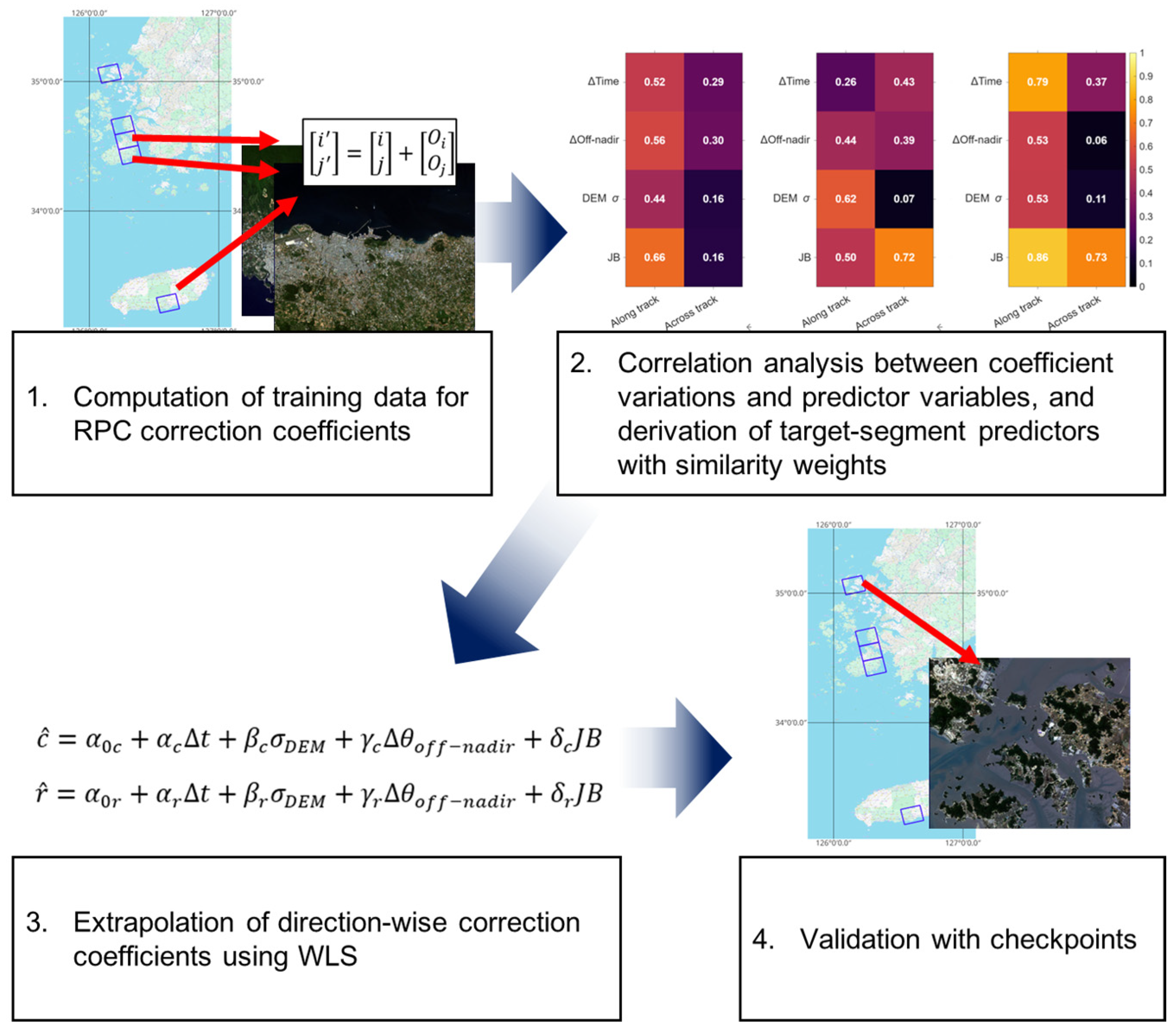
The suggested module in this research estimates and transports strip-segment RPC correction coefficients while preserving the native imaging geometry. Inputs are the head-of-strip images with their GCPs, platform metadata, and DEM tiles. We derive a compact predictor set that reflects the directional error structure observed in pushbroom strips. The predictors are elapsed time, off-nadir evolution, and terrain morphometry summarized by σDEM and the Jarque–Bera index. For each strip and direction, we fit a similarity-weighted least squares model in which calibration scenes that are morphometrically closer to the target segment receive larger weights. The fitted relation is then used to predict correction coefficients for downstream segments. A simple domain check flags segments whose morphometry falls outside the calibration envelope and triggers weight adjustment when necessary. Figure 6 presents the procedural flow, and Section 4 evaluates the transport accuracy under a common GCP and CKP protocol. Default window sizes and weighting parameters are provided in the supplement so that the procedure can be replicated without tuning.

3. Data Preparation

3.1. Strip Image Dataset

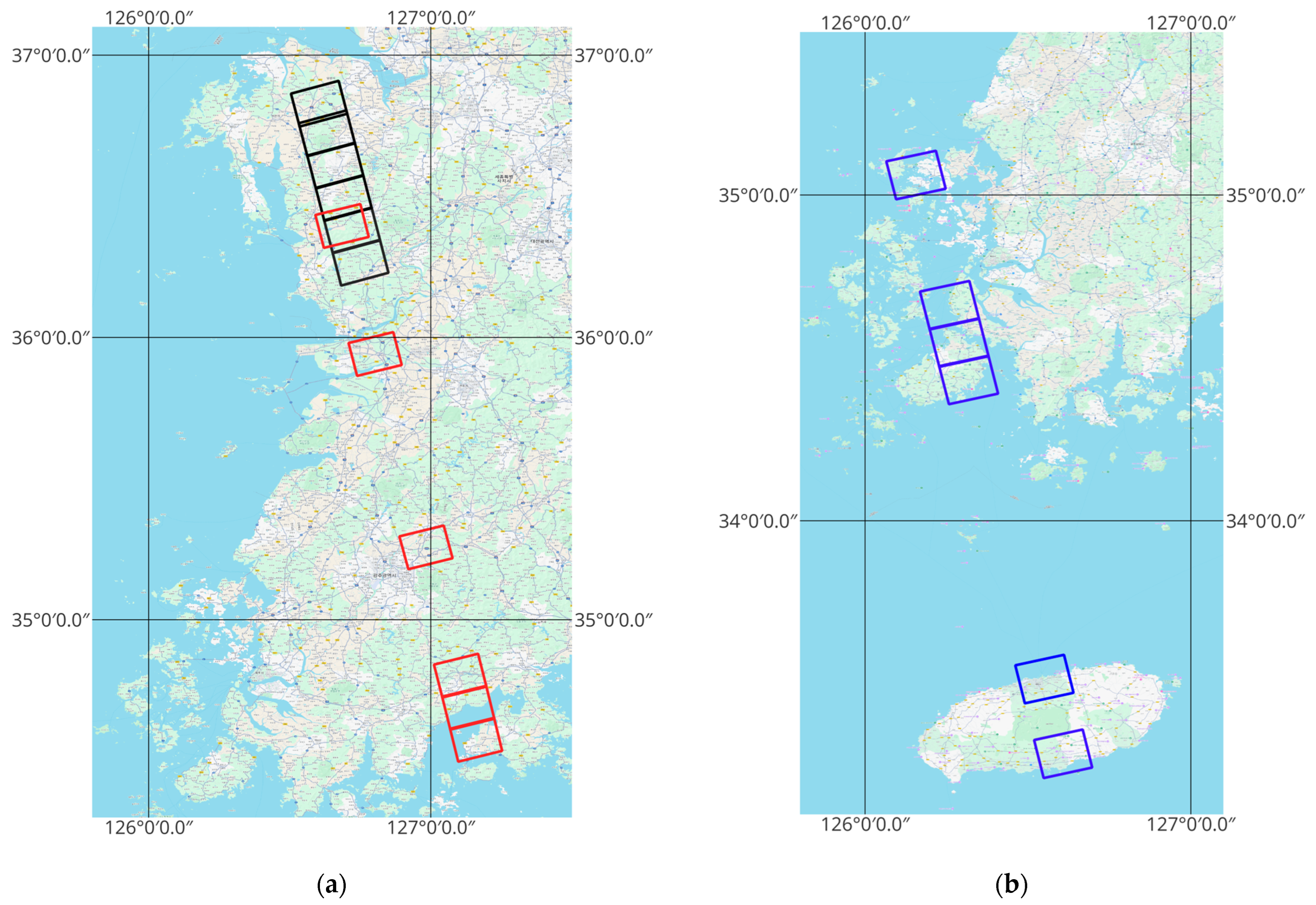
In this study, elongated strips traversing the Korean Peninsula were selected for experiments. The chosen strips had assured image quality, a cloud coverage of less than 10%, and convenient conditions for acquiring the GCPs, as shown in Figure 7. The red rectangle indicates Strip 1 (Goheung to Boryeong), the black rectangle represents Strip 2 (Seobuyeo to Dangjin), and the blue rectangle denotes Strip 3 (Seogwipo to Shinan).

Table 1. Key Parameters of the three KOMPSAT-3A Strips.

Strip Number	Target Location	Temporal Change (s)	Satellite Altitude Change (m)	Off-Nadir Change (deg)	σ of Target Area DEM (m)	Skewness of Target Area	Kurtosis of Target Area	JB of Target Area
Strip 1 K3A 20171021044156	Goheung	0	0	0	32.351	3.555	17.968	68.650
	Boseong	1.801	0.030	−0.004	95.683	1.348	3.757	1.960
	Miryeok	3.598	0.059	0.001	89.272	0.597	3.970	0.592
	Gwangju	10.800	0.177	0.016	116.848	1.528	4.971	3.307
	Gunsan	21.699	0.358	0.033	19.501	3.832	21.43	99.601
	Boryeong	28.898	0.480	0.040	126.879	1.066	4.023	1.398
Strip 2 K3A 20201107044626	Seobuyeo	0	0	0	109.847	0.962	3.630	1.0258
	Janggok	3.699	0.040	−0.004	95.839	2.406	11.308	23.047
	Hongseong	5.500	0.060	−0.005	68.893	1.884	6.775	7.114
	Deoksan	7.296	0.080	0.002	107.439	1.540	5.321	3.719
	Dangjin	9.000	0.099	−0.005	57.088	1.659	6.103	5.159
Strip 3 K3A 20210529045218	Seogwipo	0	0	0	355.803	1.847	6.293	6.121
	Jeju	3.601	0.032	−0.003	128.563	1.352	3.878	2.021
	Uisin	18.301	0.167	−0.004	73.002	2.170	7.868	10.634
	Gunnae	20.102	0.184	−0.003	54.921	3.222	15.171	47.417
	Hwawon	22.000	0.201	−0.005	41.416	2.855	11.797	27.498
	Shinan	28.402	0.262	−0.005	22.003	4.120	26.125	150.664

summarizes the key parameters of each strip. Because parameters, such as temporal and altitude changes, were calculated relative to the first image of each strip, the parameters for the initial imagery were set to 0.

3.2. DEM, Orthophoto, and Digital Map

3.2.1. ASTER GDEM V2

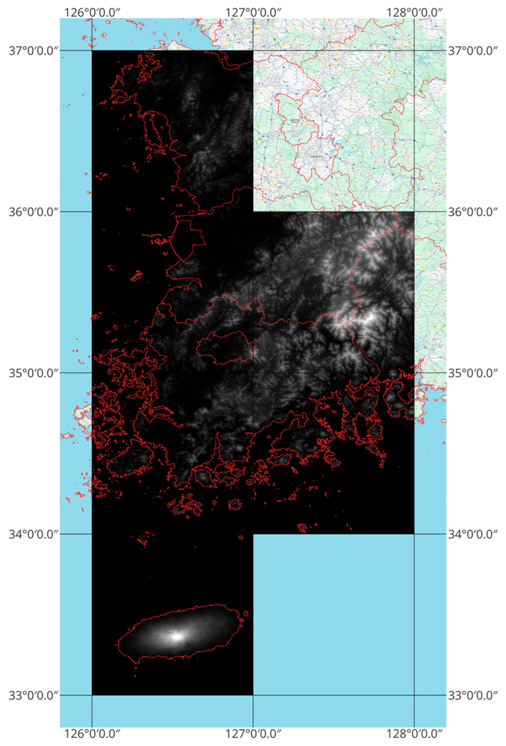
In this study, a terrain-independent method was adopted to generate RPCs. To reflect the terrain variability of the target area adequately, the minimum and maximum altitude constraints for the virtual grid were defined using the DEM of the region. The ASTER GDEM V2, provided by the National Aeronautics and Space Administration (NASA), served as the input DEM. ASTER GDEM V2 has a verified vertical accuracy, demonstrating an average error of approximately −0.2 m [39]. Figure 8 shows the full extent of ASTER GDEM V2 used in this study. ASTER GDEM V2, covering 33°N to 36°N and 126°E to 127°E, was used.

3.2.2. Digital Map and Aerial Orthophoto

Digital maps produced by the National Geographic Information Institute (NGII) of the Republic of Korea are electronic cartographic products. Based on the survey results, they depicted diverse forms of spatial information, such as terrestrial locations, topography, and place names. These data are represented using standardized symbols, textual annotations, and attributes in accordance with established cartographic scales. The NGII disseminates these digital maps and other diverse spatial datasets through the National Geographic Information Platform. Digital maps are available at scales from 1:1000 to 1:25,000. This study utilized Digital Map 2.0 at a 1:5000 scale. This specific map product has a documented positional accuracy of 1.5 m horizontally and 1.5 m vertically, assessed at a 95% confidence level [40]. To support the analysis, the contour line layer was extracted from Digital Map 2.0. Subsequently, a local DEM with a spatial resolution of 50 cm was generated using a Triangulated Irregular Network interpolation based on the extracted contours.

For the acquisition of GCPs, aerial orthoimage data produced by the NGII were utilized. This aerial orthophoto features spatial resolutions of 12 cm in urban areas and 25 cm in general areas, and its horizontal positional accuracy corresponds to that of a 1:5000 scale digital map [40].

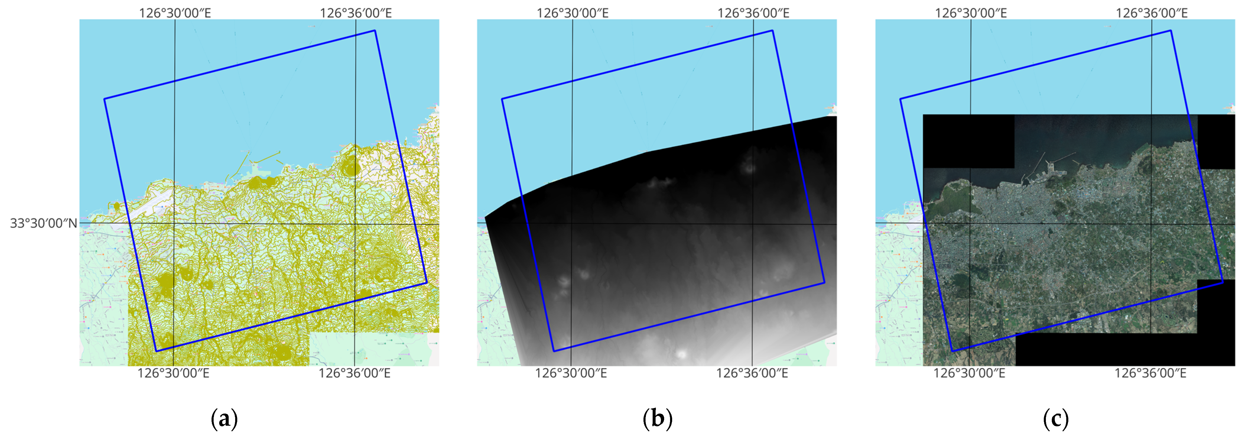
Figure 9 displays (a) the contour lines from Digital Map 2.0 covering the Jeju area, (b) the resultant local DEM, and (c) an aerial orthoimage of the same region. The blue rectangle represents the coverage extent of the satellite image, while the orange area illustrates the corresponding digital map. The detailed methodology for acquiring GCPs is described in Section 3.3.

3.3. GCPs and CKPs

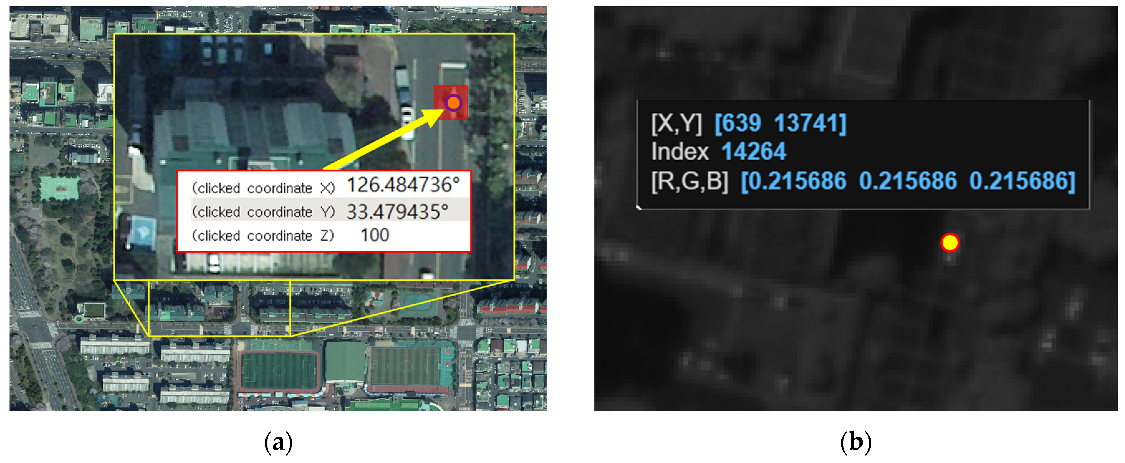
As described in Section 2, RPCs were generated using virtual GCPs, virtual images, and a terrain-independent model. For this purpose, the strip images and ASTER GDEM V2 presented in Section 3.1 and Section 3.2 were utilized. Accurate GCPs are required to derive the correction coefficients for adjusting these RPCs. In this study, a 0.5 m resolution DEM and aerial orthophotos, as detailed in Section 3.2.2, were employed to acquire these GCPs. Figure 10 briefly illustrates the procedure for obtaining GCPs.

The required number of GCPs varies according to the applied image correction model. Specifically, one GCP is sufficient for the image translation model (2-parameter), whereas two and three GCPs are necessary for the shift and drift model (4-parameter) and the affine transformation model (6-parameter), respectively. Previous studies demonstrated that employing an image translation model generally yields sufficient correction accuracy for KOMPSAT-3A satellite imagery. Therefore, this study adopted an image-translation model. However, 15 GCPs were acquired for each image to confirm error patterns and ensure redundancy. In this study, the GCPs were explicitly used to generate an RPC correction model based on the initial four images in each strip. The subsequent images within each strip were used only as CKPs to validate the extrapolated RPC correction coefficients.

4. Results and Discussion

4.1. Results of RPC Correction Coefficient Estimation and Influencing Factors

Using the terrain-independent model, the RPCs and the corresponding RPC correction coefficients were computed for six images in Strip 1, five images in Strip 2, and six images in Strip 3. The results are summarized in

Table 2. Image space error and RPC correction coefficients for each strips.

Strip 1 (Goheung–Boryeong Strip)
	Goheung	Boseong	Miryeok	Gwangju	Gunsan	Boryeong
Mean across-track error	32.36	40.09	46.76	42.63	33.95	31.00
Mean along-track error	14.64	18.25	32.55	37.65	34.25	17.13
Across-track correction coefficient	32.34	39.99	30.23	37.65	33.92	30.94
Along-track correction coefficient	11.40	7.08	−25.19	0.16	28.82	13.98
Strip 2 (Seobuyeo–Dangjin Strip)
	Seobuyeo	Janggok	Hongseong		Deoksan	Dangjin
Mean across-track error	31.95	30.32	23.80		31.34	32.07
Mean along-track error	11.37	7.30	9.23		6.60	16.86
Across-track correction coefficient	31.82	30.22	30.23		31.27	31.85
Along-track correction coefficient	−10.27	−6.19	−9.19		−5.85	−12.22
Strip 3 (Seogwipo–Shinan Strip)
	Seogwipo	Jeju	Uisin	Gunnae	Hwawon	Shinan
Mean across-track error	19.38	24.71	23.13	21.23	21.48	17.80
Mean along-track error	33.05	2.11	31.39	37.80	48.79	42.65
Across-track correction coefficient	19.35	24.68	23.02	21.12	21.45	17.74
Along-track correction coefficient	−32.81	−30.75	−31.35	−37.70	−38.70	−42.59

. Each table presents the mean across-track and along-track errors for each strip in the first two rows and the two parameters of the image translation model in the last two rows. Interestingly, despite the three strips being acquired at different times and over distinct geographic regions, the error dispersion within each strip was markedly smaller in the across-track direction than in the along-track direction. This finding is in line with earlier studies [14,41] reporting that KOMPSAT-3A imagery exhibits systematic biases of the order of several tens of pixels in the across-track direction. The across-track bias has been documented to range from approximately 20 to 31 pixels, depending on the specific scene; apart from a few images acquired over areas such as Boseong and Miryeok, this magnitude is broadly consistent with the errors quantified in the present study.

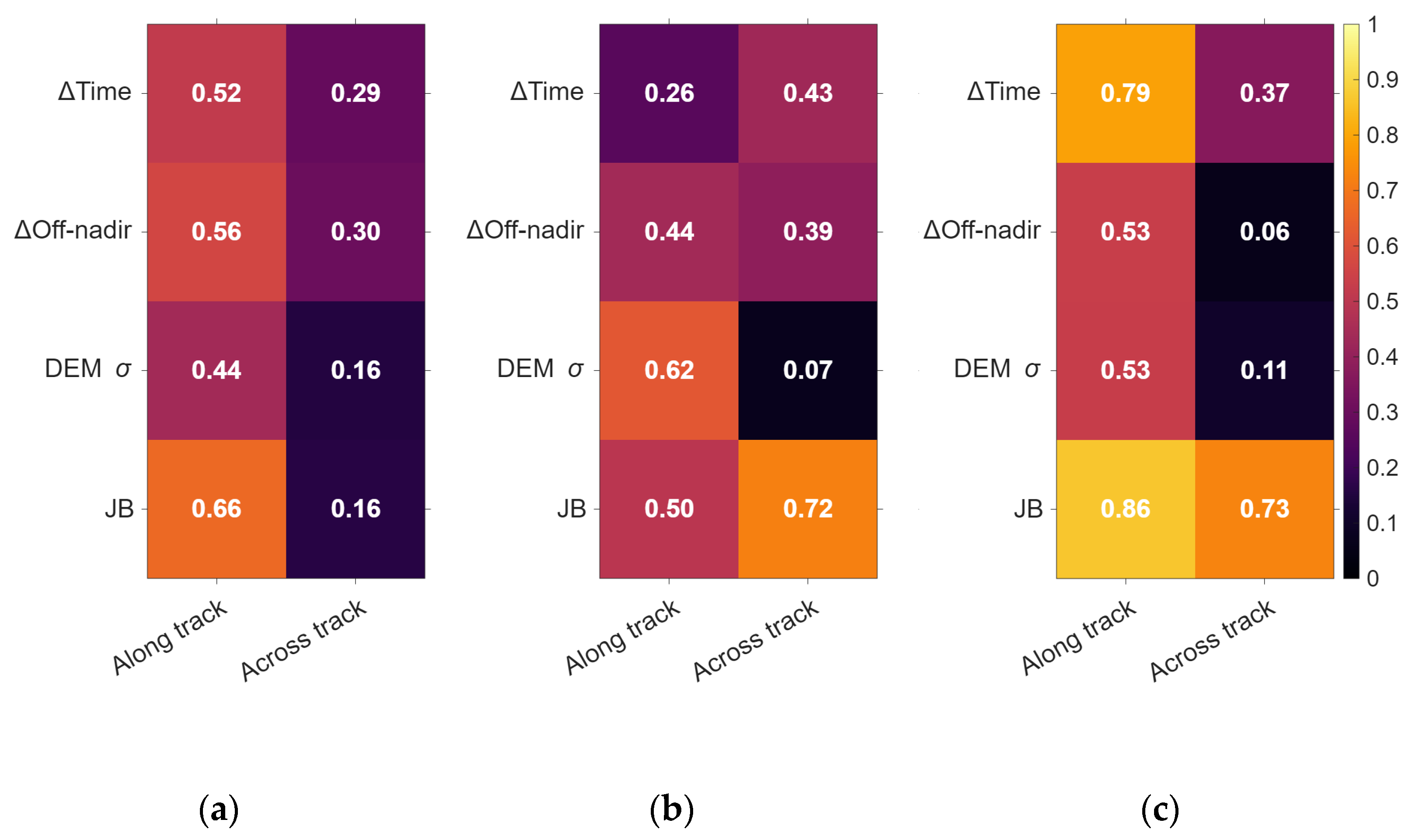
Correlation analysis was conducted between the representative satellite orbital and terrain parameters and the RPC correction coefficient variations in both the along-track and across-track directions for each strip image. To enhance interpretability, the resulting correlations were visualized using heat maps, as shown in Figure 11. A correlation analysis was conducted using Pearson’s correlation coefficients. Correlation analysis was conducted using the Pearson correlation coefficient for image-level samples within each strip; the sample sizes were n_S1 = 6, n_S2 = 5, and n_S3 = 6.

Figure 11 summarizes the stripwise Pearson correlations between the parameter changes and RPC correction coefficients. In Strip 1 (Goheung–Boryeong), both geometry-related variables dominate the along-track term: Δt and Δθ_off-nadir (r ≈ 0.52, ≈ 0.56), followed by JB (r ≈ 0.66) and a moderate σ_DEM (r ≈ 0.44). By contrast, the across-track term showed only weak associations. In Strip 2 (Seobuyeo–Dangjin), the along-track coefficient relates most strongly to σ_DEM (r ≈ 0.62), with JB (r ≈ 0.50) and Δθ_off-nadir (r ≈ 0.44) providing secondary signal, while Δt is small (r ≈ 0.26). The across-track direction is best explained by JB (r ≈ 0.72), with Δt modest (r ≈ 0.43) and Δθ_off-nadir (r ≈ 0.39) comparable, whereas σ_DEM is negligible (r ≈ 0.07). In Strip 3 (Seogwipo–Shinan), the along-track term is highly correlated with JB (r ≈ 0.86) and Δt (r ≈ 0.79), and shows moderate associations with Δθ_off-nadir (r ≈ 0.53) and σ_DEM (r ≈ 0.53). The across-track term is chiefly controlled by JB (r ≈ 0.73), while the geometry-based variables are weak (Δt r ≈ 0.37, Δθ_off-nadir r ≈ 0.06, σ_DEM r ≈ 0.11).

Consistent with these patterns, strip- and direction-specific predictors were adopted as follows: For Strip 1, the along-track model used Δθ_off-nadir and JB, whereas the across-track model used only a constant term. For Strip 2, the along-track model used σ_DEM, and the across-track model used JB. For Strip 3, the along-track model used JB and Δt, and the across-track model used JB. These choices match the dominant correlations in each panel of Figure 11, while keeping the parameterization compact for RPC correction modeling.

4.2. Extrapolation Modeling of RPC Correction Coefficients

Using the correlation coefficients derived in Section 4.1, an extrapolation model is developed to estimate the RPC correction coefficients. The model was parameterized using the temporal variation, off-nadir angle change, and local DEM standard deviation extracted from the first four images of each strip. The parameters were estimated using the weighted least-squares method, and the results are summarized in

Table 3. Extrapolation model for each strip.

Strip	Extrapolation Model
Strip 1 (Goheung–Boryeong)	$$\begin{gathered} \widehat{c}=-6.835+0.315JB \\ \widehat{r}=35.530 \end{gathered}$$
Strip 2 (Seobuyeo–Dangjin)	$$\begin{gathered} \widehat{c}=-13.728+0.047{\sigma }_{DEM}+0.184JB \\ \widehat{r}=28.743+0.027{\sigma }_{DEM}-0.053JB \end{gathered}$$
Strip 3 (Seogwipo–Shinan)	$$\begin{gathered} \widehat{c}=-26.086-0.567\Delta t-0.004JB \\ \widehat{r}=21.731+0.007\Delta t-0.016JB \end{gathered}$$

. This extrapolation model was constructed by excluding the last image of each strip and utilizing the remaining images to formulate a prediction function.

Table 4. Comparative Table of Estimated RPC Correction Parameters.

Strip	Test Area	Direction	Estimated Correction Coefficient (pix)	Reference Correction Coefficient (pix)	Correction Coefficient Errors (pix)
Strip 1	Boryeong	Across track	35.530	30.941	4.589
		Along track	16.358	13.981	2.377
Strip 2	Dangjin	Across track	30.026	31.849	1.823
		Along track	−10.068	−12.223	2.155
Strip 3	Shinan	Across track	19.558	17.736	1.822
		Along track	−42.353	−42.585	0.232

GSD; Strip 1: 0.637 m, Strip 2: 0.710 m, Strip 3: 0.710 m.

presents a comparative assessment of the estimated RPC correction coefficients against their corresponding reference values across the representative test sites in Strips 1-3. The results are reported separately for the along-track and across-track components together with the absolute prediction errors expressed in pixels.

In Strip 1 (Boryeong), the estimated across-track correction coefficient was 35.530 pixels, compared with the reference value of 30.941 pixels, yielding an error of 4.589 pixels. The along-track coefficient was 16.358 pixels versus the reference value of 13.981 pixels, with an error of 2.377 pixels. In Strip 2 (Dangjin), the across-track coefficient was 30.026 pixels, relative to the reference of 31.849 pixels, with an error of 1.823 pixels. The along-track coefficient is −10.068 pixels compared to the reference of −12.223 pixels, resulting in an error of 2.155 pixels. In Strip 3 (Shinan), the across-track coefficient was 19.558 pixels relative to a reference of 17.736 pixels, with an error of 1.822 pixels. The along-track coefficient is −42.353 pixels compared to the reference of −42.585 pixels, with an error of 0.232 pixels.

Table 5. RPC correction errors (pixels) for along- and across-track components at selected distances across strips.

Strip	Test Area	Distance (km)	Along-Track Error (pix)	Across-Track Error (pix)
Strip 1	Gunsan	77.717	9.706	1.345
	Boryeong	129.147	1.345	4.865
Strip 2	Deoksan	12.995	3.924	0.328
	Dangjin	129.147	2.658	1.879
Strip 3	Hwawon	12.993	4.803	1.373
	Shinan	58.309	12.577	1.550

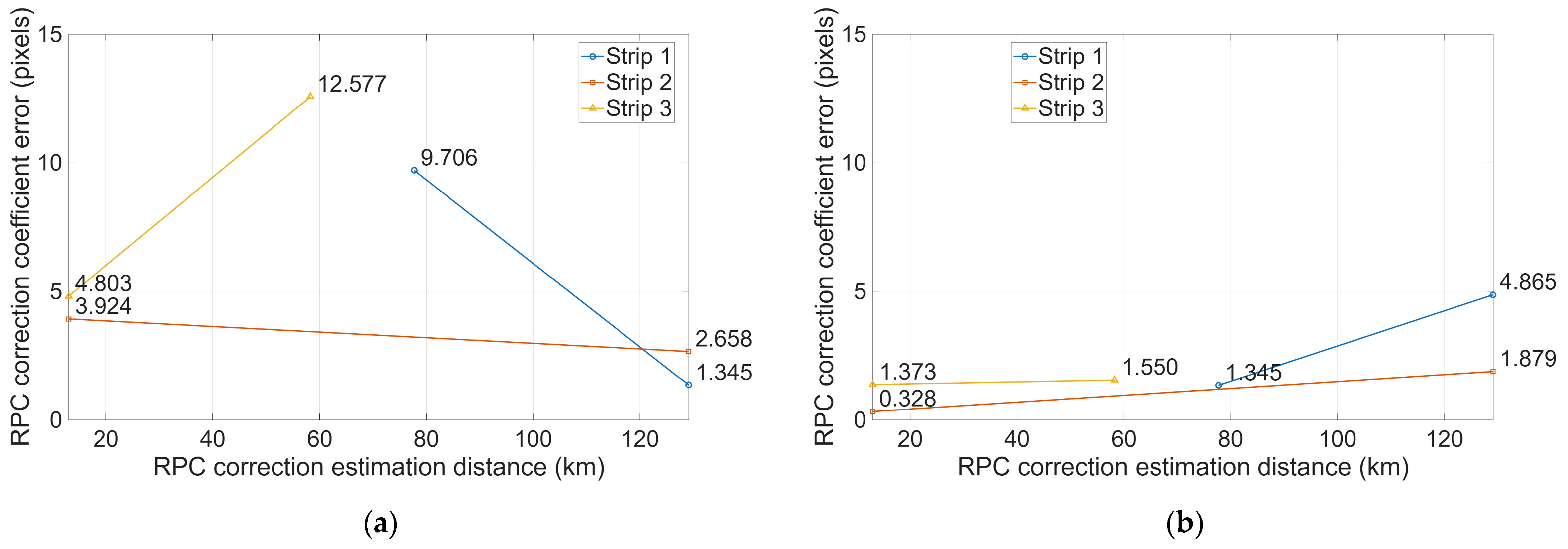
GSD; Strip 1: 0.637 m, Strip 2: 0.710 m, Strip 3: 0.710 m.

presents the errors of the extrapolated RPC correction parameters at selected distances for Strips 1-3, and Figure 12 graphically illustrates these results. To secure longer extrapolation distances, unlike previous experiments, the extrapolation model was trained by excluding the last two images, and the accuracy was verified using these final two images. In Strip 1, the extrapolated RPC correction parameters yielded an along-track error of 9.706 pixels and an across-track error of 1.345 pixels at 77.717 km, while at 129.147 km, the along-track error was 1.345 pixels, and the across-track error was 4.865 pixels. In Strip 2, the errors at 12.995 km were 3.924 pixels along the track and 0.328 pixels across the track, whereas at 129.147 km, the errors were 2.658 and 1.879 pixels, respectively. In Strip 3, the errors at 12.993 km were 4.803 along the track and 1.373 pixels across the track, and at 58.309 km, the corresponding errors were 12.577 and 1.550 pixels.

4.3. Comparative Evaluation of RPC Correction Approaches

Lee et al. [42] proposed an alternative approach for long-strip KOMPSAT-3A imagery, in which the entire strip is represented by a single RPC rather than by generating multiple scene-based RPCs, as in conventional methods. To achieve this, they first analyzed variations in satellite attitude, specifically roll and pitch, using a physical sensor model and then simplified these variations as linear motion to enable stable RPC generation across extended strips. More specifically, virtual ground control points were created from satellite orbit and attitude data and used to estimate a single RPC for the entire strip. In this process, the original image strip is transformed by incorporating the linearized attitude information, after which the RPC is regenerated. In this study, the RPC correction coefficients for strip imagery were derived using both Lee’s method and the proposed approach. Because Lee’s method considers the entire strip as a single image and computes a single RPC, it is particularly suitable for connected-strip data. Therefore, a comparison was conducted using only the Seobuyeo–Dangjin strip.

For the entire Seobuyeo–Dangjin strip, RPCs were generated and subsequently refined using GCPs to derive the RPC correction coefficients.

Table 6. Residual errors at Deoksan and Dangjin checkpoints for the Seobuyeo–Dangjin strip.

	Previous Approach RPC Correction Coefficient Error		Proposed Approach RPC Correction Coefficient Error
	Along-Track Error	Across-Track Error	Along-Track Error	Across-Track Error
Deoksan	4.644	0.059	3.924	0.328
Dangjin	2.801	1.794	2.658	1.879

GSD; Strip 2: 0.710 m.

presents the residual errors at the Deoksan and Dangjin checkpoints when both the previous and proposed approaches were applied. In the across-track direction, both approaches yielded small errors of approximately one pixel or less at Deoksan, although the error at Dangjin was nearly two pixels. By contrast, the along-track errors were consistently larger, exceeding 2.6 pixels in all cases. The proposed approach slightly reduced the along-track errors compared with the previous method while maintaining comparable performance in the across-track direction.

5. Discussion

5.1. RPC Correction Behavior and Influencing Factors

The observed first-order structure of the correction coefficients across the three strips reflects the intrinsic geometry of the pushbroom imaging. In the across-track direction, the residuals converge into nearly constant biases, whereas in the along-track direction, they are driven by long-period drifts that accumulate with acquisition time. These contrasting behaviors, quantified in Table 2, indicate distinct physical origins: boresight and orbital systematic errors form constant terms across the detector array, whereas attitude drift progressively enlarges the residuals along the line-scanning axis.

The strip-specific patterns reinforce this interpretation. In Strip 2, the across-track bias remained stable within a narrow range of approximately 30 pixels, whereas the along-track variation was moderate. Strip 3 shows consistent across-track stability between 17 and 25 pixels, but also exhibits a clear along-track drift of −30 to −43 pixels, amplified in its mountainous section where elevation variability and the JB are high. As the strip transitions to the coastal lowlands, the error regime shifts back toward across-track bias dominance. In contrast, Strip 1 maintains a constant across-track bias between 31 and 47 pixels, but registers the largest along-track fluctuations, consistent with strong cumulative drift.

The variable-level correlations in Figure 11 further highlight the directional dependencies. While along-track errors are generally explained by elapsed time Δt and off-nadir variation Δθ_off-nadir, Strip 1 is dominated by JB, indicating the sensitivity of this higher-order morphometric index to steep terrain. In Strip 2, along-track errors were most closely tied to σ_DEM, and across-track residuals showed the strongest association with JB. In Strip 3, the along-track component is influenced by both Δt and JB, whereas the across-track component is again primarily governed by JB. Collectively, these findings suggest that JB effectively captures extreme elevation events in coastal environments and on steep mountain slopes. It regulates fine-scale systematic deviations around the across-track bias, and modulates or amplifies long-period drifts in the along-track direction. The consistency between the stripwise correction coefficients in Table 2 and the correlation structures in Figure 11 provides evidence for this interpretation.

5.2. Extrapolation Models and Performance of RPC Corrections

The models in Table 3 operationalize the correlation patterns in Figure 11 by selecting minimal predictor sets with coefficients above 0.6 and by applying a JB-centered Gaussian kernel weighting that has a greater influence on calibration scenes morphometrically similar to the target. JB is a dimensionless index that captures cliffs, ridges, and other extreme elevation events even under identical σ_DEM, which makes it an effective domain-adaptive weight. Along-track formulations use Δt and Δθ_off-nadir as primary drivers with JB or σ_DEM as amplifiers, while across-track formulations pair a constant term with JB to absorb constant bias and fine-scale systematics. The signs and magnitudes of the selected predictors mirror Figure 11, and similarity weighting reduces extrapolation variance while preserving parsimony and physical interpretability across heterogeneous terrain.

Table 4 lists the stability and failure modes. One scene in Strip 2 remains within approximately three pixels in both directions, and the terminal scene in Strip 3 approaches the reference with a sub-pixel along-track error, indicating consistent geometry and a good domain match between the training and target. By contrast, the Boryeong scene in Strip 1 shows a severe across-track error despite a moderate across-track error. This breakdown arises from an out-of-distribution Δθ_off-nadir spectrum between training and validation together with an abrupt rise in σ_DEM. In pushbroom geometry, along-track residuals accumulate with Δt and low-frequency drift in Δθ_off-nadir, and terrain variability magnifies parallax, so a Δθ_off-nadir spectrum shift combined with a terrain regime shift produces large residuals. The across-track errors remain relatively constrained by the constant-bias structure of the sensor.

Table 5 and Figure 12 show that errors do not follow a monotonic law with distance or Δt. Trajectories differ by direction and by strip because distance interacts with the Δθ_off-nadir profile, spatial variation in JB and σ_DEM, and scene-specific kernel weights. Therefore, distance alone is neither necessary nor sufficient for reliability assessment. A practical methodology is to precompute Δθ_off-nadir, JB, and σ_DEM for the target and to apply similarity-weighted extrapolation to secure domain fit and stabilize prediction.

5.3. Comparative Discussion with Other Approaches

Prior work [42] argued that generating a single strip-wide RPC without explicitly treating attitude variation can produce large errors because the RPC does not capture substantial changes in satellite attitude. To mitigate this, Lee et al. fitted the roll-pitch trajectory to a linear function and resected a strip-level RPC on the linearized geometry. In contrast, the present study retains the native scene geometry and extrapolates the correction coefficients from a compact, physically interpretable set of predictors that encode time evolution, off-nadir variation, and terrain morphometry with similarity weighting. The former approach reshapes the imaging dynamics such that one RPC can explain the full strip, whereas the latter transports calibrated coefficients to the target segment in a domain-aware manner without requiring continuous tie coverage.

The contrast between these two strategies is both conceptual and operational. The replacement model route seeks to reshape the image geometry so that a single RPC can explain the full strip once the roll pitch is linearized. The performance depends on how well the linear motion hypothesis matches the actual attitude trajectory and on the availability of reliable ephemeris and reference chips for every scene in the strip. The extrapolation route preserves the original scene geometry and carries forward correction coefficients through predictors that represent the time, viewing, and terrain regimes. Performance depends on the predictor coverage and the quality of the similarity weights, rather than on the global linearization of attitude.

These differences have practical consequences for the along- and across-track components that dominate stripwise behavior. The previous approach is effective in compressing the attitude-induced variability into a form that a single RPC can absorb. This is most advantageous when the strip exhibits clear low-frequency attitude drifts that are well-approximated by linear functions, as reflected in the improvement reported for the unstable segments. The extrapolation method in this work acts directly on the terms that generate drift and transport corrections to the downstream end, where the cumulative effects are the largest. In the experiments in this study, the along-track component benefited from this targeted modeling, whereas the across-track component remained governed by a near-constant bias that could be tuned, if needed, with a lightweight offset.

These two methods differ in terms of their data dependence and robustness. The replacement model strategy presumes access to the ephemeris and sufficient image chips to support resection across the full strip, and can be less forgiving when segments are missing or when the strip is delivered as disjoint parts. The predictor-driven extrapolation in this study does not require uninterrupted or continuous-tie information. It can be trained on available upstream calibration scenes and applied to downstream targets, even when portions of the strip are unavailable, which is valuable in operational settings where acquisitions are interrupted or partially redacted.

Taken together, previous work shows that linearizing the attitude and regenerating a strip-level RPC is an effective pathway when the platform dynamics admit a simple motion model and full-strip references are accessible. The present approach shows that extrapolating correction coefficients using physically grounded predictors and morphometric similarity weighting is a complementary pathway that emphasizes transportability, interpretability, and resilience to missing segments. In applications that demand continuity across interrupted strips or the rapid extension of calibrations to the tail of a long acquisition, the extrapolation framework offers a direct and operationally flexible means of controlling the along-track drift while preserving the simple bias structure across tracks.

6. Conclusions

This study addresses the limitations of a single strip-wide RPC under significant attitude variations by preserving the native scene geometry and extrapolating the RPC correction coefficients to downstream segments from a compact set of physically interpretable predictors. Elapsed time and off-nadir evolution represent low-frequency drivers of along-track drift, and a morphometric similarity weight anchored by terrain statistics moderates the sensitivity to local extremes. This approach targets the mechanism of error transport rather than reshaping the imaging model, which enables its use when ground control is sparse or segments are missing.

Experiments using three KOMPSAT-3A strips confirmed the directional structure discussed in this study. Across the track, the residual behaved as a near-constant bias. Along the track, the residual followed a slowly varying drift that accumulated with time and attitude evolution. Applied to downstream segments, the model reduced positional errors in Strips 2 and 3 to under 3 pixels, which corresponds to approximately 1.65–1.7 m at a ground sampling distance of 0.55 m. Strip 1 exhibited larger residuals of roughly 6 pixels due to attitude drift exceeding the calibration envelope. This outcome indicates the need for broader acquisition-time coverage and, where telemetry supports it, the possible inclusion of higher-order or nonlinear terms for aggressive maneuvers.

Compared with strip-level replacement models that linearize roll and pitch and then estimate a single RPC for the entire strip, the present framework infers and transports correction coefficients directly from predictors that encode time, view, and terrain regimes. The replacement route is effective when the attitude evolution is well-approximated by a simple motion model and when reliable ephemerides and reference image chips are available. The proposed approach emphasizes the transportability, interpretability, and robustness to interrupted or partially redacted strips. It requires only a small set of head scenes, supports domain checking through similarity weights, and allows any residual across-track bias to be removed with a lightweight offset rather than a full model refit.

Future studies will prioritize focused validation. As KOMPSAT-7 has not yet been launched, the workflow will be prepared for immediate application during its early commissioning, and representative strips will be calibrated as soon as they become available. For CAS500-1, the same procedure was applied for programmatic access to the suitable strips. The objective was to confirm portability without reparametrizing the predictor set. Both platforms employ AEISS-derived sensor architectures similar to KOMPSAT-3A; therefore, the geometric structure and systematic error patterns are expected to be consistent, supporting the direct extension of the proposed approach. Telemetry indicates a mid-strip change in drift, and a lightly regularized shift-and-drift variant is evaluated as a drop-in extension, whereas the translation model remains the default for routine production.

References

1. Chen, J.; Dowman, I.; Li, S.; Li, Z.; Madden, M.; Mills, J.; Paparoditis, N.; Rottensteiner, F.; Sester, M.; Toth, C. Information from Imagery: ISPRS Scientific Vision and Research Agenda. ISPRS J. Photogramm. Remote Sens. 2016, 115, 3–21. [Google Scholar] [CrossRef]
2. Li, J.; Huang, X.; Tu, L.; Zhang, T.; Wang, L. A Review of Building Detection from Very High Resolution Optical Remote Sensing Images. GISci. Remote Sens. 2022, 59, 1199–1225. [Google Scholar] [CrossRef]
3. Mukhopadhyay, A.; Pal, I.; Hati, J.P.; Pramanick, N.; Acharyya, R.; Kumar, A.; Jana, S.K.; Mitra, D. High-Resolution Pléiades Data: An in-Depth Analysis of Applications and Future Prospects. Spat. Inf. Res. 2024, 32, 739–755. [Google Scholar] [CrossRef]
4. Shen, X.; Liu, B.; Li, Q.-Q. Correcting Bias in the Rational Polynomial Coefficients of Satellite Imagery Using Thin-Plate Smoothing Splines. ISPRS J. Photogramm. Remote Sens. 2017, 125, 125–131. [Google Scholar] [CrossRef]
5. Ban, S.; Kim, T. Rational-Function-Model-Based Rigorous Bundle Adjustment for Improving the Relative Geometric Positioning Accuracy of Multiple Korea Multi-Purpose Satellite-3A Images. Remote Sens. 2024, 16, 2890. [Google Scholar] [CrossRef]
6. Berthier, E.; Lebreton, J.; Fontannaz, D.; Hosford, S.; Belart, J.M.-C.; Brun, F.; Andreassen, L.M.; Menounos, B.; Blondel, C. The Pléiades Glacier Observatory: High-Resolution Digital Elevation Models and Ortho-Imagery to Monitor Glacier Change. Cryosphere 2024, 18, 5551–5571. [Google Scholar] [CrossRef]
7. Pan, H.; Zou, S.; Guan, L. Block Adjustment with Drift Compensation for Rational Function Model. Photogramm. Eng. Remote Sens. 2018, 84, 791–799. [Google Scholar] [CrossRef]
8. Clermont, L.; Michel, C.; Stockman, Y. Stray Light Correction Algorithm for High Performance Optical Instruments: The Case of Metop-3MI. Remote Sens. 2022, 14, 1354. [Google Scholar] [CrossRef]
9. Clermont, L.; Michel, C.; Chouffart, Q.; Zhao, Y. Going beyond Hardware Limitations with Advanced Stray Light Calibration for the Metop-3MI Space Instrument. Sci. Rep. 2024, 14, 19490. [Google Scholar] [CrossRef]
10. Shen, X.; Li, Q.; Wu, G.; Zhu, J. Bias Compensation for Rational Polynomial Coefficients of High-Resolution Satellite Imagery by Local Polynomial Modeling. Remote Sens. 2017, 9, 200. [Google Scholar] [CrossRef]
11. Noh, M.-J.; Howat, I.M. Applications of High-Resolution, Cross-Track, Pushbroom Satellite Images with the SETSM Algorithm. IEEE J. Sel. Top. Appl. Earth Obs. Remote Sens. 2019, 12, 3885–3899. [Google Scholar] [CrossRef]
12. Rizeei, H.M.; Pradhan, B. Urban Mapping Accuracy Enhancement in High-Rise Built-up Areas Deployed by 3D-Orthorectification Correction from WorldView-3 and LiDAR Imageries. Remote Sens. 2019, 11, 692. [Google Scholar] [CrossRef]
13. Ghuffar, S. DEM Generation from Multi Satellite Planetscope Imagery. Remote Sens. 2018, 10, 1462. [Google Scholar] [CrossRef]
14. Jo, H.; Lee, C.; Oh, J. The Impact of GCP Chip Distribution on Kompsat-3A RPC Bias Compensation. Appl. Sci. 2024, 14, 3482. [Google Scholar] [CrossRef]
15. Loghin, A.-M.; Otepka-Schremmer, J.; Pfeifer, N. Potential of Pléiades and WorldView-3 Tri-Stereo DSMs to Represent Heights of Small Isolated Objects. Sensors 2020, 20, 2695. [Google Scholar] [CrossRef]
16. Huang, W.; Zhang, G.; Tang, X.; Li, D. Compensation for Distortion of Basic Satellite Images Based on Rational Function Model. IEEE J. Sel. Top. Appl. Earth Obs. Remote Sens. 2016, 9, 5767–5775. [Google Scholar] [CrossRef]
17. Yang, B.; Wang, M.; Xu, W.; Li, D.; Gong, J.; Pi, Y. Large-Scale Block Adjustment without Use of Ground Control Points Based on the Compensation of Geometric Calibration for ZY-3 Images. ISPRS J. Photogramm. Remote Sens. 2017, 134, 1–14. [Google Scholar] [CrossRef]
18. Pi, Y.; Yang, B.; Li, X.; Wang, M.; Cheng, Y. Large-Scale Planar Block Adjustment of GaoFen1 WFV Images Covering Most of Mainland China. IEEE Trans. Geosci. Remote Sens. 2018, 57, 1368–1379. [Google Scholar] [CrossRef]
19. Dai, R.; Wang, M.; Ye, Z. Near-Real-Time Long-Strip Geometric Processing without GCPs for Agile Push-Frame Imaging of LuoJia3-01 Satellite. Remote Sens. 2024, 16, 3281. [Google Scholar] [CrossRef]
20. Hong, Z.; Tong, X.; Liu, S.; Chen, P.; Xie, H.; Jin, Y. A Comparison of the Performance of Bias-Corrected RSMs and RFMs for the Geo-Positioning of High-Resolution Satellite Stereo Imagery. Remote Sens. 2015, 7, 16815–16830. [Google Scholar] [CrossRef]
21. Xiong, Z.; Zhang, Y. A Generic Method for RPC Refinement Using Ground Control Information. Photogramm. Eng. Remote Sens. 2009, 75, 1083–1092. [Google Scholar] [CrossRef]
22. Topan, H.; Oruc, M.; Taşkanat, T.; Cam, A. Combined Efficiency of RPC and DEM Accuracy on Georeferencing Accuracy of Orthoimage: Case Study with Pléiades Panchromatic Mono Image. IEEE Geosci. Remote Sens. Lett. 2013, 11, 1148–1152. [Google Scholar] [CrossRef]
23. Toutin, T. Geometric Processing of Remote Sensing Images: Models, Algorithms and Methods. Int. J. Remote Sens. 2004, 25, 1893–1924. [Google Scholar] [CrossRef]
24. Li, Q.; Zhong, R.; Yang, C.; Zhao, K.; Zhang, C.; Li, Y. Geometric Quality Improvement Method of Optical Remote Sensing Satellite Images Based on Rational Function Model. Remote Sens. 2022, 14, 4443. [Google Scholar] [CrossRef]
25. Titarov, P.S. Evaluation of Cartosat 1 Geometric Potential. In Proceedings of the XXI ISPRS Congress, Beijing, China, 3 July 2008; pp. 841–846. [Google Scholar]
26. Liu, H.; Zhao, Y.; Wang, L.; Liu, Y. Comparison of DEM Accuracies Generated from Different Stereo Pairs over a Plateau Mountainous Area. J. Mt. Sci. 2021, 18, 1580–1590. [Google Scholar] [CrossRef]
27. Fraser, C.S.; Baltsavias, E.; Gruen, A. Processing of Ikonos Imagery for Submetre 3D Positioning and Building Extraction. ISPRS J. Photogramm. Remote Sens. 2002, 56, 177–194. [Google Scholar] [CrossRef]
28. Seo, D.; Oh, J.; Lee, C.; Lee, D.; Choi, H. Geometric Calibration and Validation of Kompsat-3A AEISS-A Camera. Sensors 2016, 16, 1776. [Google Scholar] [CrossRef]
29. Pan, H.; Huang, T.; Zhou, P.; Cui, Z. Self-Calibration Dense Bundle Adjustment of Multi-View Worldview-3 Basic Images. ISPRS J. Photogramm. Remote Sens. 2021, 176, 127–138. [Google Scholar] [CrossRef]
30. Eftekhari, A.; Saadatseresht, M.; Motagh, M. A Study on Rational Function Model Generation for TerraSAR-X Imagery. Sensors 2013, 13, 12030–12043. [Google Scholar] [CrossRef] [PubMed]
31. Schneider, M.; Baumgartner, A.; Schwind, P.; Carmona, E.; Storch, T. Differences and Similarities in the Processing of Airborne and Spaceborne Hyperspectral Data Shown on HySpex and EnMap Processing Chains. In Proceedings of the IGARSS 2019—2019 IEEE International Geoscience and Remote Sensing Symposium, Yokohama, Japan, 28 July–2 August 2019; pp. 9164–9167. [Google Scholar] [CrossRef]
32. Yeom, J.-M.; Ko, J.; Hwang, J.; Lee, C.-S.; Choi, C.-U.; Jeong, S. Updating Absolute Radiometric Characteristics for KOMPSAT-3 and KOMPSAT-3A Multispectral Imaging Sensors Using Well-Characterized Pseudo-Invariant Tarps and Microtops II. Remote Sens. 2018, 10, 697. [Google Scholar] [CrossRef]
33. Seo, D.-C.; Lee, C.; Oh, J. Merge of Sub-Images from Two PAN CCD Lines of Kompsat-3 AEISS. KSCE J. Civ. Eng. 2016, 20, 863–872. [Google Scholar] [CrossRef]
34. Kim, N.; Choi, Y.; Bae, J.; Sohn, H.-G. Estimation and Improvement in the Geolocation Accuracy of Rational Polynomial Coefficients with Minimum GCPs Using KOMPSAT-3A. GISci. Remote Sens. 2020, 57, 719–734. [Google Scholar] [CrossRef]
35. EOS Data Analytics. KOMPSAT 3/3A Satellite Images. Available online: https://eos.com/find-satellite/kompsat-3-3a/#:~:text=Pan%20CCD%20detector%20module (accessed on 21 June 2025).
36. Hu, Y.; Tao, V.; Croitoru, A. Understanding the Rational Function Model: Methods and Applications. Int. Arch. Photogramm. Remote Sens. 2004, 20, 119–124. [Google Scholar]
37. Tao, C.V.; Hu, Y. A Comprehensive Study of the Rational Function Model for Photogrammetric Processing. Photogramm. Eng. Remote Sens. 2001, 67, 1347–1358. [Google Scholar]
38. Fraser, C.S.; Dial, G.; Grodecki, J. Sensor Orientation via RPCs. ISPRS J. Photogramm. Remote Sens. 2006, 60, 182–194. [Google Scholar] [CrossRef]
39. Tachikawa, T.; Kaku, M.; Iwasaki, A.; Gesch, D.B.; Oimoen, M.J.; Zhang, Z.; Danielson, J.J.; Krieger, T.; Curtis, B.; Haase, J. ASTER Global Digital Elevation Model Version 2-Summary of Validation Results. USGS Rep. 2011, 37. Available online: https://ui.adsabs.harvard.edu/abs/2011usgs.rept...37T/abstract (accessed on 20 September 2025).
40. Regulations on the Work and Performance of Digital Topographic Maps. Available online: https://www.law.go.kr/LSW//admRulLsInfoP.do?admRulId=37114&efYd=0 (accessed on 10 May 2025).
41. Oh, J.H.; Seo, D.C.; Lee, C.N. A Test Result on the Positional Accuracy of Kompsat-3A Beta Test Images. J. Korean Soc. Surv. Geod. Photogramm. Cartogr. 2016, 34, 133–142. [Google Scholar] [CrossRef]
42. Lee, C.; Seo, D.; Jung, J.; Oh, J. Replacement Sensor Model Generation for a Long High-Resolution Satellite Image Strip. KSCE J. Civ. Eng. 2023, 27, 1751–1759. [Google Scholar] [CrossRef]
Figure 1. Flowchart of the research.
Remotesensing 17 03332 g001
Figure 2. The configuration of the AEISS-A panchromatic CCD sensor on KOMPSAT-3A.
Remotesensing 17 03332 g002
Figure 3. Coordinate transformation process of KOMPSAT-3A.
Remotesensing 17 03332 g003
Figure 4. Input data for RPC generation: (a) DEM of the target area; (b) virtual grid from DEM; (c) virtual image from virtual grid.
Remotesensing 17 03332 g004
Figure 5. Correlation between the off-nadir angle and the satellite’s attitude angles: (a) strong positive correlation case (Goheung–Boryeong strip); (b) a strong negative correlation case (Seogwipo–Shinan strip).
Remotesensing 17 03332 g005
Figure 6. Flowchart of the proposed RPC correction coefficient extrapolation procedure.
Remotesensing 17 03332 g006
Figure 7. KOMPSAT-3A strip overview: (a) Red boxes: Goheung–Boryeong strip; Black boxes: Seobuyeo–Dangjin strip; (b) Blue boxes: Seogwipo–Shinan strip.
Remotesensing 17 03332 g007
Figure 8. Visualization of ASTER GDEM v2 covering the strip regions.
Remotesensing 17 03332 g008
Figure 9. Aerial Orthophoto and Digital Map Samples: (a) Digital map of Jeju area (1:5000); (b) 50 cm resolution DEM derived from the digital map; (c) 25 cm resolution aerial photograph of Jeju area.
Remotesensing 17 03332 g009
Figure 10. Examples of GCP Acquisition: (a) Obtaining geographic coordinates and elevation; (b) Obtaining image coordinates.
Remotesensing 17 03332 g010
Figure 11. Heat map of Pearson correlation coefficients between parameter changes and RPC correction coefficient variations (along-track and across-track) for each strip: (a) Strip 1; (b) Strip 2; (c) Strip 3.
Remotesensing 17 03332 g011
Figure 12. RPC correction coefficient errors (pixels) as a function of estimation distance for Strips 1-3; (a) Along-track errors, (b) Across-track errors.
Remotesensing 17 03332 g012