Author Contributions
Conceptualization, M.M. and D.S.; methodology, M.M.; software, M.M.; validation, M.M.; formal analysis, M.M.; investigation, M.M. and D.S.; resources, D.S. and J.F.; data curation, M.M.; writing—original draft preparation, M.M.; writing—review and editing, D.S. and J.F.; visualization, M.M.; supervision, D.S. and J.F.; project administration, D.S. and J.F.; funding acquisition, D.S. and J.F. All authors have read and agreed to the published version of the manuscript.
Figure 1.
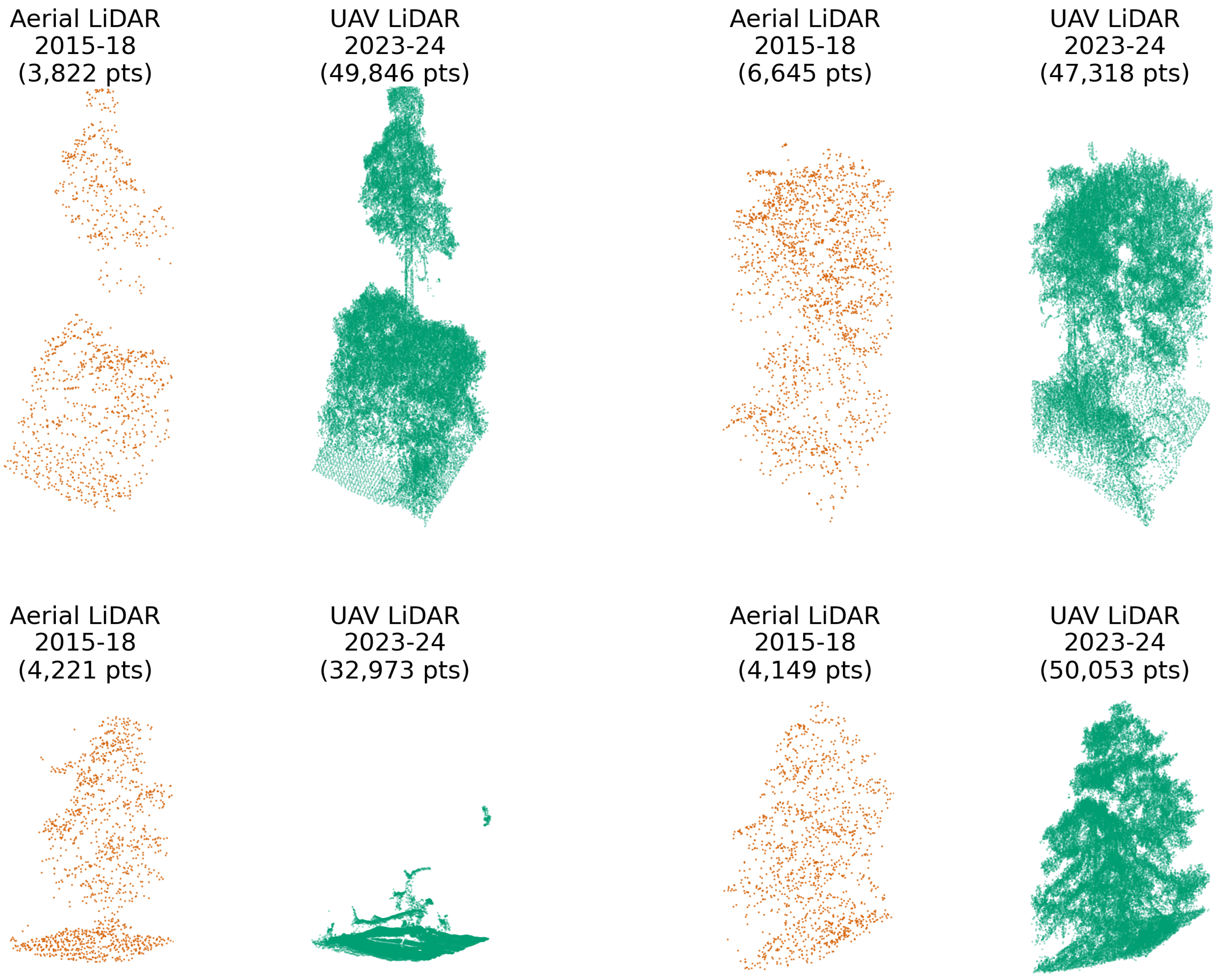
Comparison of point clouds with 10 m × 10 m footprints from USGS 3DEP aerial LiDAR (2015–2018, orange) and UAV LiDAR (2023–2024, green) over the same locations. UAV LiDAR captures significantly greater structural detail, especially in fine-scale canopy features. The bottom-left example shows clear canopy loss between surveys due to recent disturbance. The top left shows clear growth.
Figure 2.
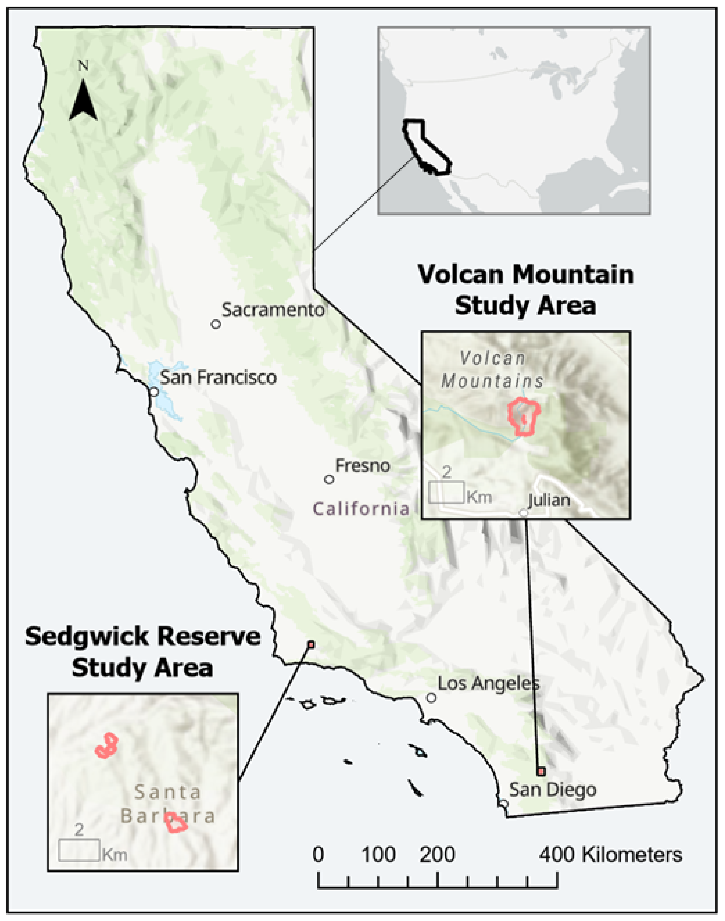
Locations of the Southern California UAV LiDAR surveys—Sedgwick Reserve–Midland School in the Santa Ynez Valley and Volcan Mountain Wilderness Preserve in the Peninsular Range. Red outlines indicate the extent of the UAV LiDAR surveys.
Figure 2.
Locations of the Southern California UAV LiDAR surveys—Sedgwick Reserve–Midland School in the Santa Ynez Valley and Volcan Mountain Wilderness Preserve in the Peninsular Range. Red outlines indicate the extent of the UAV LiDAR surveys.
Figure 3.
The first study area combines parts of the Sedgwick Reserve and Midland School property in the San Rafael Mountain foothills, Santa Barbara County. It features diverse vegetation, such as oak woodlands, chaparral, grasslands, and coastal sage scrub. Within this area, four UAV LiDAR sites were surveyed, covering a total of 70 hectares. The numbers indicate the UAV LiDAR survey sites which are detailed in
Table 1.
Figure 4.
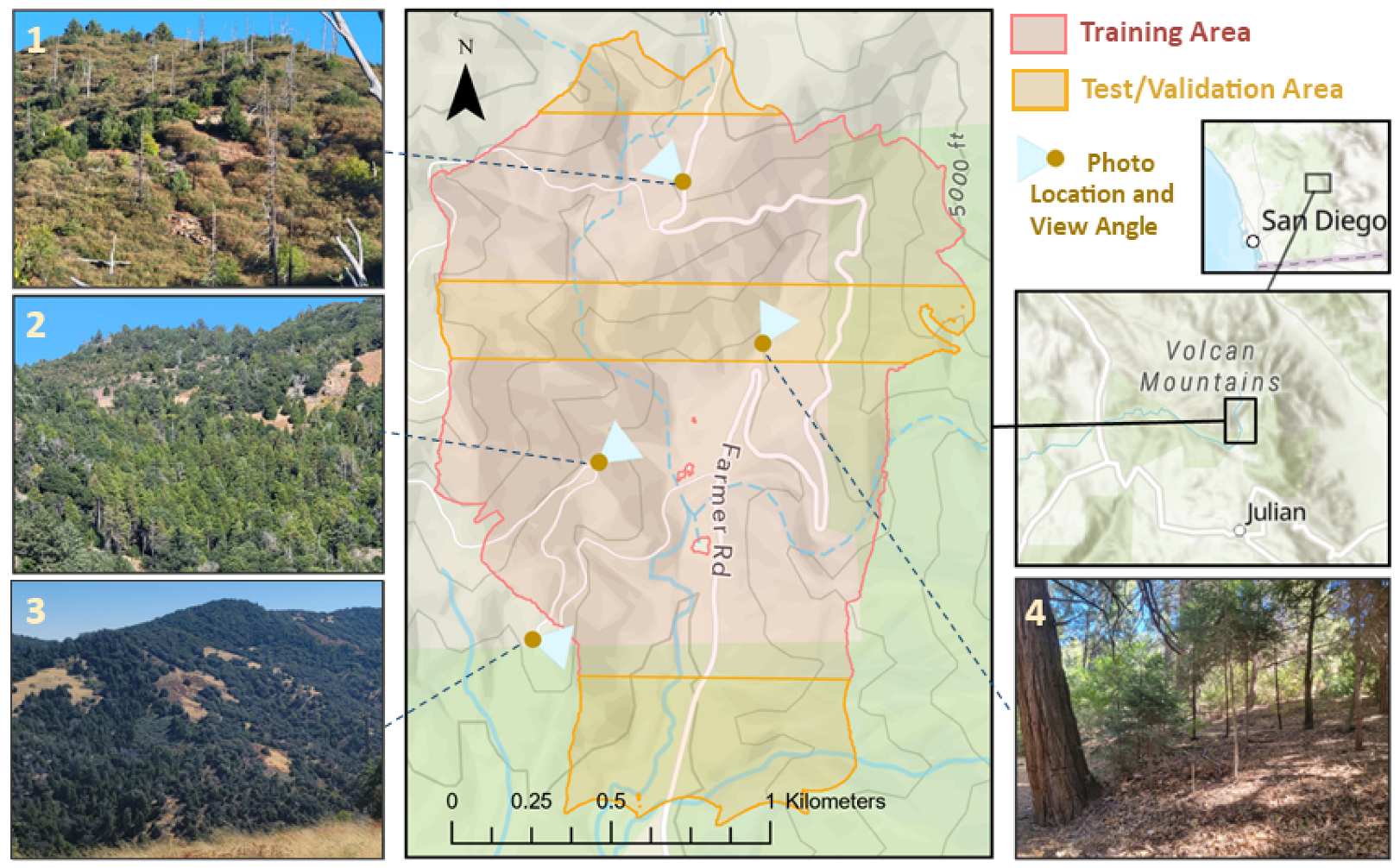
Volcan Mountain study area (197 hectares) in the Peninsular Range of Southern California, encompassing diverse vegetation types across an elevation range of 1220 to 1675 m. Thirty percent of the site (58 hectares) was set aside for testing/validation in three zones: post-fire chaparral in the north, mixed conifer and riparian vegetation with oak and chaparral in the center, and oak woodland with semi-continuous canopy in the south. Subfigures 1, 2, 3, 4 show photos of the different vegetation types in the study area.
Figure 5.
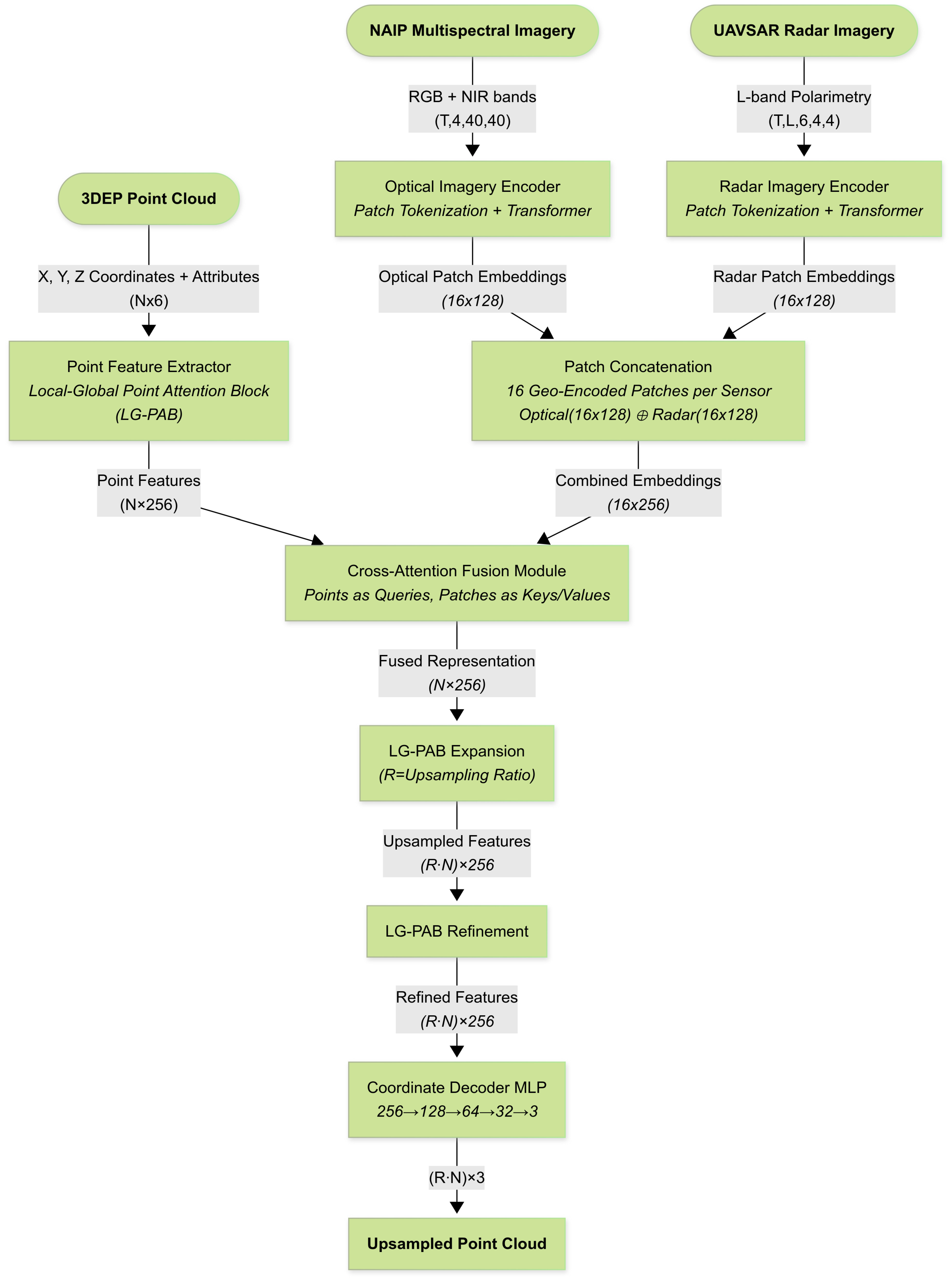
The overall multi-modal upsampling architecture. Key components include local–global point attention blocks, modality-specific imagery encoders for the processing of optical (NAIP) and radar (UAVSAR) data, and a cross-attention fusion module for combining imagery and LiDAR features.
Figure 5.
The overall multi-modal upsampling architecture. Key components include local–global point attention blocks, modality-specific imagery encoders for the processing of optical (NAIP) and radar (UAVSAR) data, and a cross-attention fusion module for combining imagery and LiDAR features.
Figure 6.
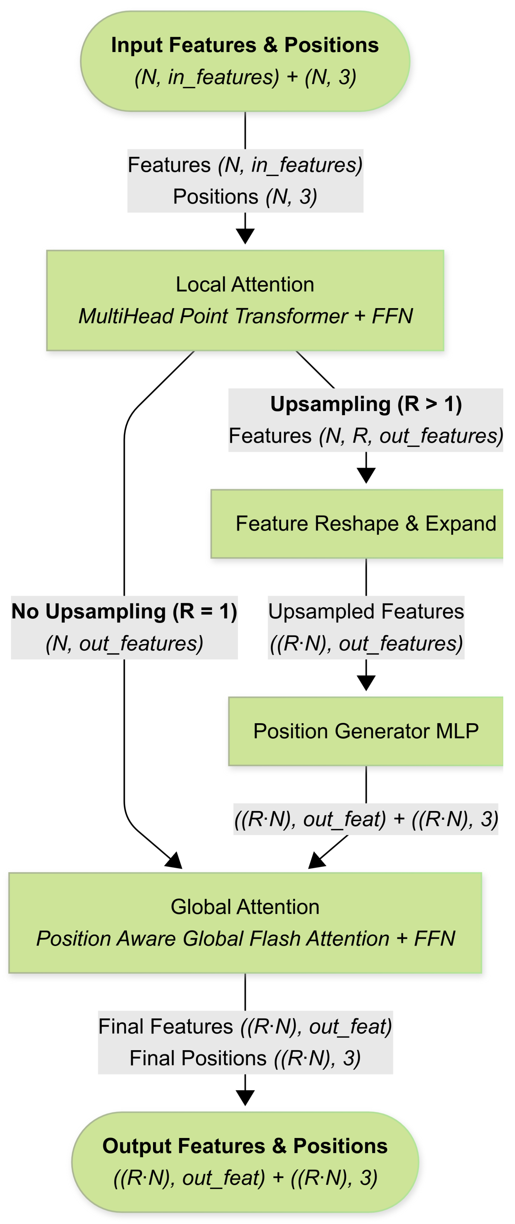
Flow chart of the Local–Global Point Attention Block (LG-PAB), the core computational unit used across the feature extraction, expansion, and refinement stages. The block applies local attention via a multi-head point Transformer, optional upsampling with learned position offsets, and global multi-head FlashAttentionfor broader spatial context. A feed-forward MLP follows both the local and global attention blocks.
Figure 7.
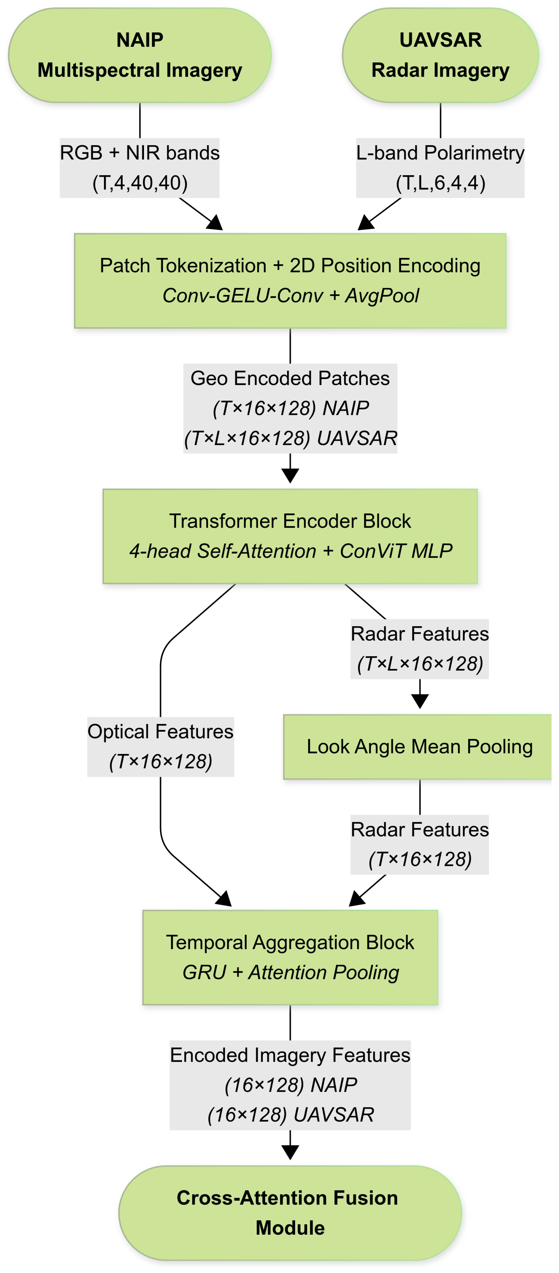
Architectural diagram of the imagery encoders. Image stacks from NAIP (optical) and UAVSAR (radar) pass sequentially through patch tokenization, Transformer encoder blocks for spatial context modeling, and a temporal GRU-Attention head for temporal aggregation.
Figure 7.
Architectural diagram of the imagery encoders. Image stacks from NAIP (optical) and UAVSAR (radar) pass sequentially through patch tokenization, Transformer encoder blocks for spatial context modeling, and a temporal GRU-Attention head for temporal aggregation.
Figure 8.
Distribution of Chamfer distance (CD) reconstruction errors comparing raw input data to the 3DEP LiDAR-only baseline model, each evaluated against the reference. Horizontal boxplots show the median (red line), interquartile range (colored boxes), and 10th–90th percentile whiskers; outliers beyond the 90th percentile are excluded. The baseline model shows a lower median CD (0.340 m vs. 0.858 m) with a tighter distribution. (Note: CD can vary with sampling density and point counts; since the input and predictions (2× upsampled) differ in size relative to the reference, these magnitudes are not a normalized comparison and are shown for qualitative context).
Figure 9.
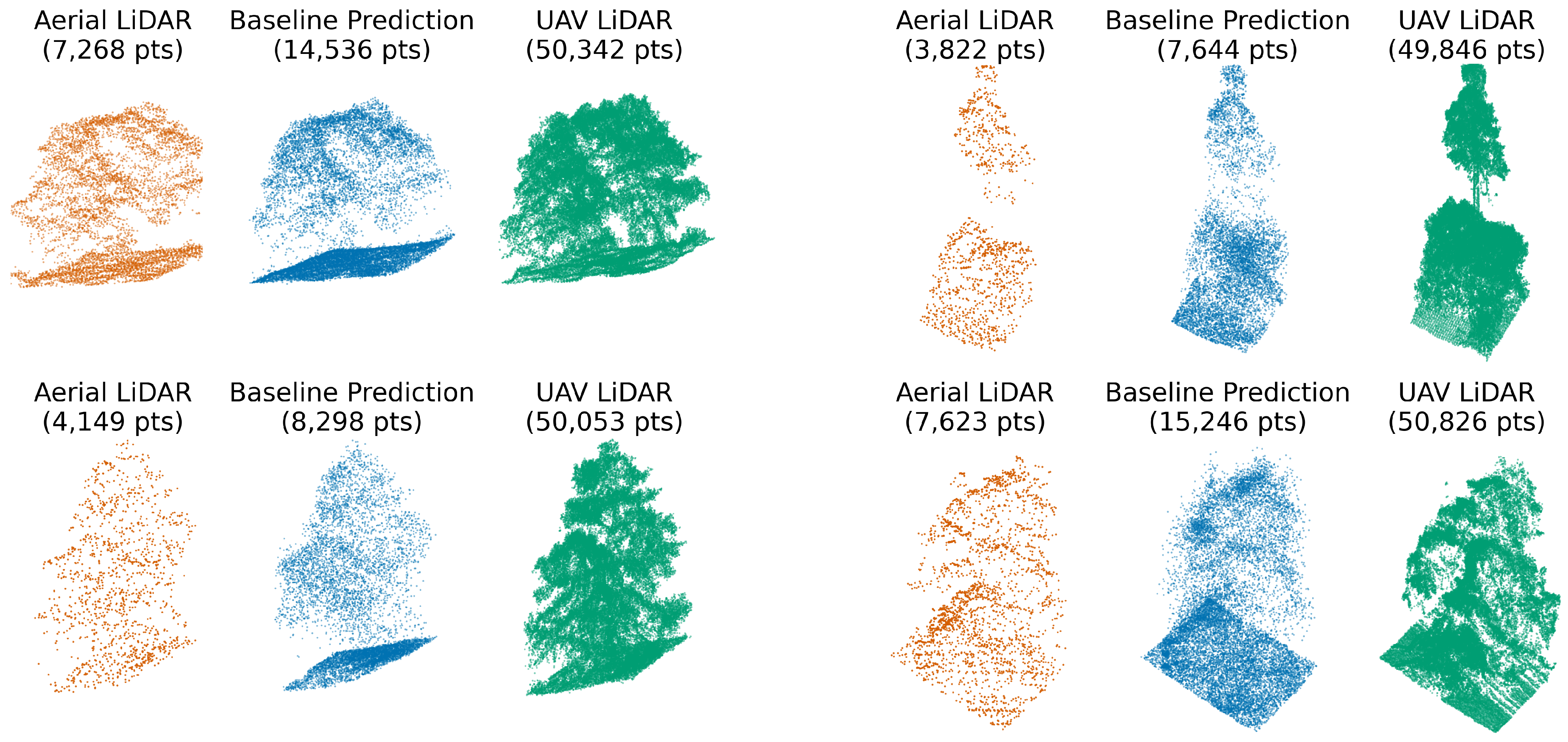
A comparison of baseline (3DEP LiDAR only) model output vs. input.
Figure 9.
A comparison of baseline (3DEP LiDAR only) model output vs. input.
Figure 10.
Distribution of Chamfer distance reconstruction errors across point-cloud upsampling models. Horizontal box plots show median (red line), interquartile range (colored boxes), and 10th–90th percentile whiskers for models trained with different input modalities. All models demonstrate substantial improvement over the LiDAR-only baseline, with the fused model achieving the lowest median error (0.298 m) and tightest distribution. Outliers beyond the 90th percentile are excluded for clarity.
Figure 11.
Example tile where no major vegetation change occurred between the 3DEP aerial LiDAR (2015–2018) and UAV LiDAR (2023–2024). The optical + SAR fusion model more accurately recovers fine-scale canopy structure compared to the LiDAR-only model, producing a point cloud that more closely matches the UAV LiDAR reference (lower Chamfer distance).
Figure 12.
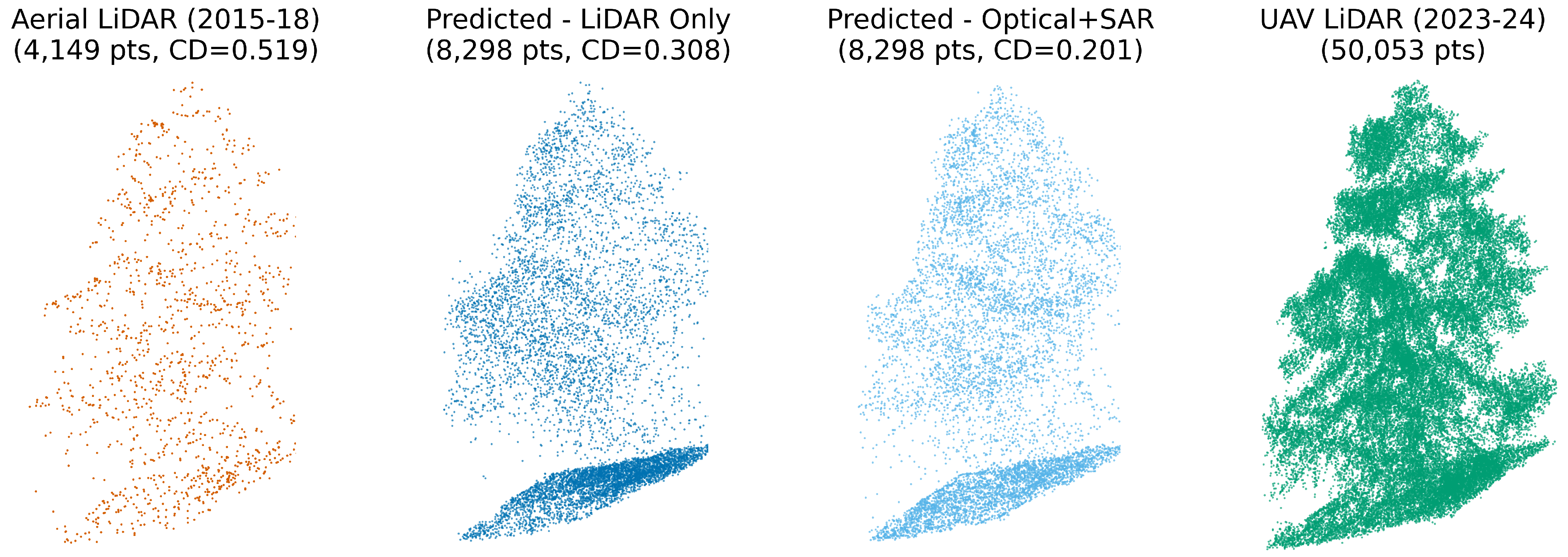
Example tile illustrating vegetation structure change between legacy aerial LiDAR (2015–2018) and recent UAV LiDAR (2023–2024). The optical + SAR fusion model accurately reconstructs the canopy loss visible in the UAV LiDAR reference, whereas the LiDAR-only model retains outdated structure from the earlier survey. This highlights the value of multi-modal imagery in correcting legacy LiDAR and detecting structural change.
Figure 13.
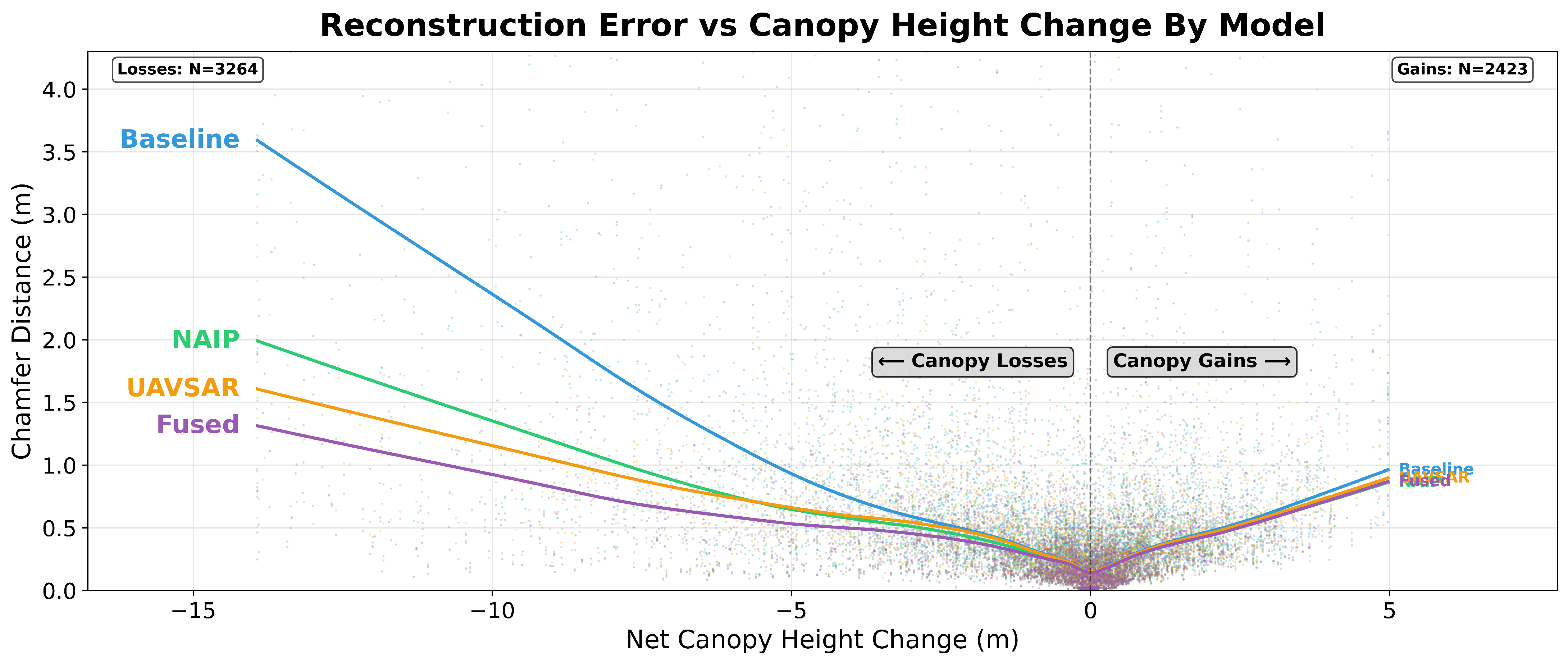
Relationship between point-cloud reconstruction error (Chamfer distance) and net canopy height change since the original LiDAR survey. Scatter points show individual sample tiles (N = 5687) with LOWESS trend lines for each model; outliers above the 99.5th percentile for both error and height change metrics were excluded for visual clarity. Negative values represent canopy losses, while positive values represent gains. The baseline model (blue) shows substantially higher error rates for large canopy losses compared to models incorporating additional remote sensing data (NAIP optical, UAVSAR radar, and fused approaches), while all models perform similarly for canopy gains.
Figure 14.
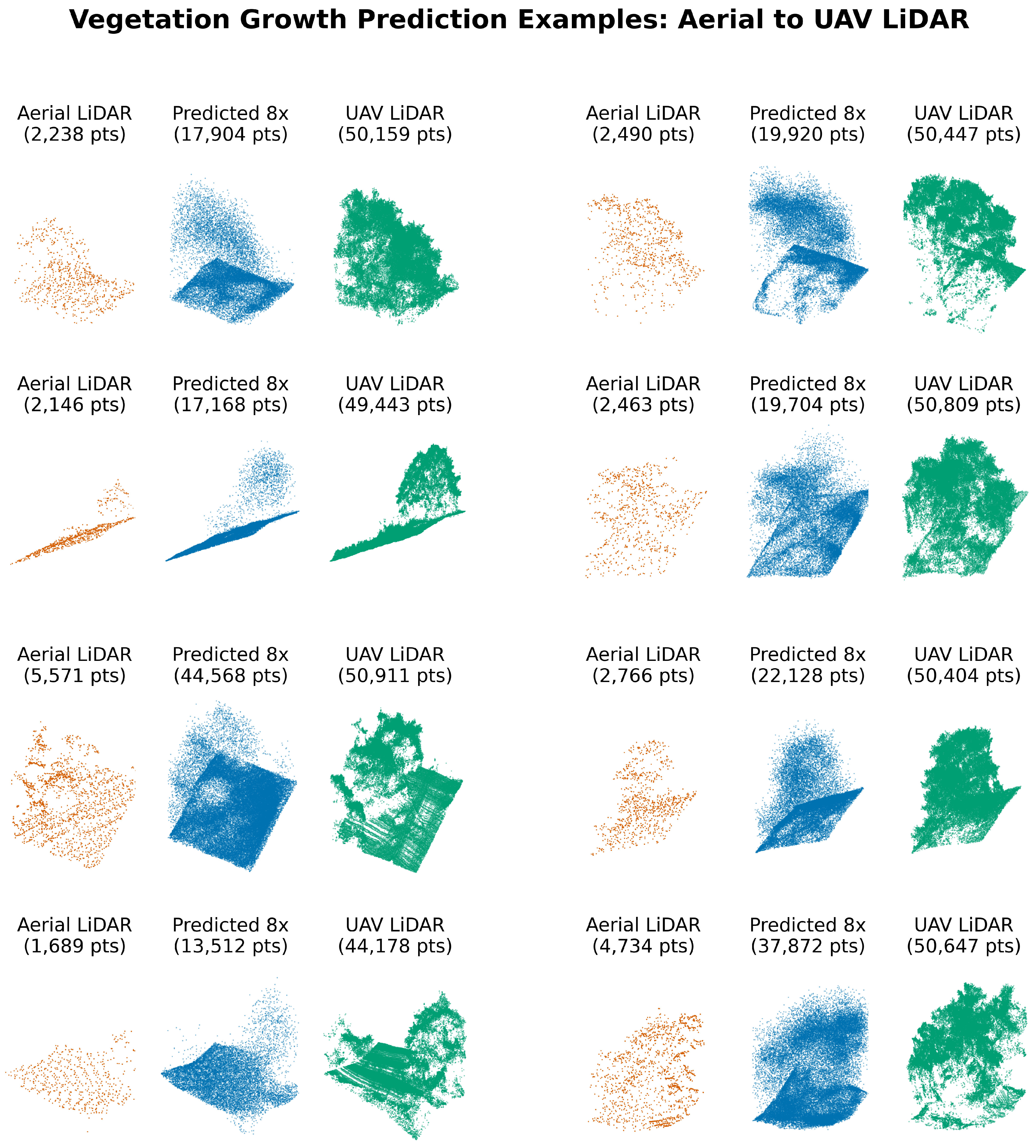
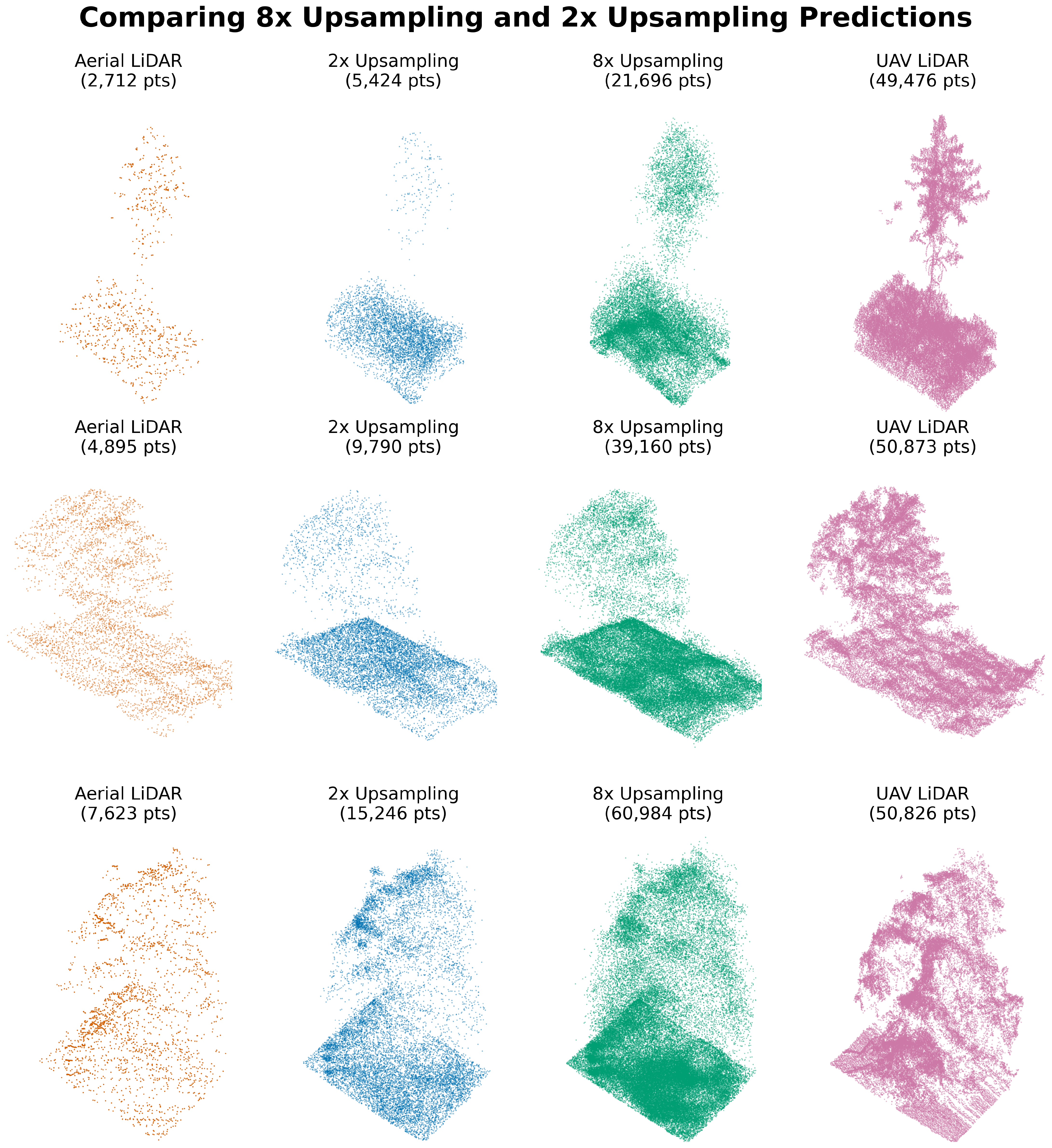
Comparison of the standard 2× upsampling model (optical + SAR, 6.8 million parameters) output versus a preliminary high-density 8× model (optical + SAR, 125 million parameters).
Figure 14.
Comparison of the standard 2× upsampling model (optical + SAR, 6.8 million parameters) output versus a preliminary high-density 8× model (optical + SAR, 125 million parameters).
Table 1.
UAV LiDAR sites used as ground truth for model development.
Table 1.
UAV LiDAR sites used as ground truth for model development.
| Site | Hectares | Location | Collection Date | Model Use |
|---|
| 1 | 38 | Sedgwick Reserve | 30 June 2023 | Training |
| 2 | 12 | Midland School | 23 October 2023 | Training |
| 3 | 9 | Midland School | 23 October 2023 | Test/Validation |
| 4 | 11 | Midland School | 28 September 2023 | Test/Validation |
| 5 | 197 | Volcan Mountain | 25 October 2024 | 70% Training
30% Test/Validation |
Table 2.
Summary of remote sensing datasets used in the data stack.
Table 2.
Summary of remote sensing datasets used in the data stack.
| Data Source | Role in Study | Details | Revisit Rate |
|---|
| UAV LiDAR | Reference Data | >300 pts/m2
Acquired: 2023–2024 | N/A 1 |
| 3DEP Airborne LiDAR | Sparse Input | Sedgwick: ∼22 pts/m2 (2018)
Volcan: ∼6 pts/m2 (2015–2016) | N/A 1 |
| UAVSAR (L-band) | Ancillary Input | 6.17 m GSD
Coverage: 2014–2024 | ∼2–3 years |
| NAIP (Optical) | Ancillary Input | 0.6–1 m GSD
Coverage: 2014–2022 | ∼2 years |
Table 3.
Timeline of NAIP and UAVSAR acquisitions for both study sites.
Table 3.
Timeline of NAIP and UAVSAR acquisitions for both study sites.
| | Volcan Mountain | Sedgwick Reserve |
|---|
|
Year
|
NAIP (GSD)
|
UAVSAR (# Looks 1)
|
NAIP (GSD)
|
UAVSAR (# Looks 1)
|
|---|
| 2014 | May (1 m) | June (3), October (2) | June (1 m) | June (8) |
| 2016 | April (60 cm) | — | June (60 cm) | April (6) |
| 2018 | August (60 cm) | October (2) | July (60 cm) | — |
| 2020 | April (60 cm) | — | May (60 cm) | — |
| 2021 | — | November (2) | — | — |
| 2022 | April (60 cm) | — | May (60 cm) | — |
| 2023 | — | — | — | September (6) 2 |
| 2024 | — | — | — | October (2) |
Table 4.
Dataset preparation.
Table 4.
Dataset preparation.
| Subset | Tiles |
|---|
| Training | 24,000 original + 16,000 augmented = 40,000 |
| Validation | 3792 |
| Test | 5688 |
Table 5.
Model variants evaluated.
Table 5.
Model variants evaluated.
| Variant | Active Encoders | Cross-Attention on | Parameters |
|---|
| Baseline | LiDAR only | None | 4.7 M |
| + NAIP | LiDAR, optical | NAIP tokens | 5.9 M |
| + UAVSAR | LiDAR, radar | UAVSAR tokens | 5.8 M |
| Fused | LiDAR, optical, radar | Concatenated token | 6.8 M |
Table 6.
Model-configuration parameters.
Table 6.
Model-configuration parameters.
| Parameter | Value | Notes |
|---|
| Core geometry | |
| Point-feature dimension | 256 | — |
| KNN neighbours (k) | 16 | Used in local attention graph |
| Upsampling ratio () | 2 | Doubles point density per LG-PAB expansion |
| Point-attention dropout | 0.02 | Dropout inside global attention heads |
| Attention-head counts | |
| Extractor — local / global | 8 / 4 | Extra local heads help expand feature set |
| Expansion — local / global | 8 / 4 | Extra local heads aid point upsampling |
| Refinement — local / global | 4 / 4 | — |
| Imagery encoders | |
| Image-token dimension | 128 | Patch embeddings for NAIP & UAVSAR encoders |
| Cross-modality fusion | |
| Fusion heads | 4 | — |
| Fusion dropout | 0.02 | — |
| Positional-encoding dimension | 36 | — |
Table 7.
Training protocol and hardware.
Table 7.
Training protocol and hardware.
| Setting | Value |
|---|
| Hardware | 4 × NVIDIA L40 (48 GB) GPUs under PyTorch DDP 2.5.1 (CUDA 12.4) DDP |
| Optimizer | ScheduleFreeAdamW [54]; base LR , weight-decay , ; no external LR schedule |
| Loss function | Density-aware Chamfer distance (Equation (9) in [55]), |
| Batch size | 15 tiles per GPU |
| Epochs | 100 |
| Gradient clip | |
| Training time | ≈ 7 h per model variant |
| Model selection | Epoch with lowest validation loss |
Table 8.
Descriptive statistics for Chamfer distance across all model variants (see
Table 5).
Table 8.
Descriptive statistics for Chamfer distance across all model variants (see
Table 5).
| Model | Mean CD (m) | Median CD (m) | Std Dev (m) | IQR (m) |
|---|
| Input | 2.568 | 0.858 | 6.852 | 1.540 |
| Baseline | 1.043 | 0.340 | 5.717 | 0.465 |
| NAIP | 0.993 | 0.316 | 5.542 | 0.421 |
| UAVSAR | 0.924 | 0.331 | 5.505 | 0.437 |
| Fused | 0.965 | 0.298 | 5.753 | 0.393 |
Table 9.
RQ1 and RQ2: Impact of single and fused modalities on reconstruction error.
Table 9.
RQ1 and RQ2: Impact of single and fused modalities on reconstruction error.
| Comparison | Median Change (%) | Effect Size |
|---|
| RQ1: Single Modality vs. Baseline |
| NAIP vs. Baseline | 0.5 (p < 0.001) | 0.088 |
| UAVSAR vs. Baseline | 0.3 (p < 0.001) | 0.062 |
| RQ2: Fused Modality vs. Best Single Modality |
| Fused vs. NAIP | 0.7 (p < 0.001) | 0.133 |
Table 10.
RQ3: Correlation between reconstruction error and canopy height change.
Table 10.
RQ3: Correlation between reconstruction error and canopy height change.
| Model | Spearman | p-Value |
|---|
| Baseline | 0.650 | p < 0.001 |
| NAIP | 0.612 | p < 0.001 |
| UAVSAR | 0.628 | p < 0.001 |
| Fused | 0.582 | p < 0.001 |
| Baseline vs. NAIP (z) | 3.377 | p < 0.001 |
| Baseline vs. UAVSAR (z) | 1.999 | p = 0.046 |
| Baseline vs. Fused (z) | 5.868 | p < 0.001 |
Table 11.
RQ3 extended: Correlation between reconstruction error and canopy height changes (gains vs. losses).
Table 11.
RQ3 extended: Correlation between reconstruction error and canopy height changes (gains vs. losses).
| Model | Canopy Gains (N = 2423) | Canopy Losses (N = 3264) |
|---|
| Spearman | p-Value | Spearman | p-Value |
|---|
| Baseline | 0.601 | p < 0.001 | 0.671 | p < 0.001 |
| NAIP | 0.586 | p < 0.001 | 0.621 | p < 0.001 |
| UAVSAR | 0.597 | p < 0.001 | 0.637 | p < 0.001 |
| Fused | 0.587 | p < 0.001 | 0.580 | p < 0.001 |
| Baseline vs. NAIP (z) | 0.825 | p = 0.409 | 3.440 | p < 0.001 |
| Baseline vs. UAVSAR (z) | 0.233 | p = 0.816 | 2.406 | p = 0.016 |
| Baseline vs. Fused (z) | 0.768 | p = 0.442 | 6.074 | p < 0.001 |
