HLAE-Net: A Hierarchical Lightweight Attention-Enhanced Strategy for Remote Sensing Scene Image Classification

Highlights

What are the main findings?

• A lightweight attention-enhanced module group for remote sensing scene image classification working with residual networks is proposed.
• A deployment scheme for the proposed attention-enhanced module group is proposed.
• An HLAE-Net for remote sensing scene image classification based on ResNet50 is proposed.

What is the implication of the main finding?

• The proposed lightweight attention-enhanced module group can improve the classification ability of large and complex remote sensing scene images on the basis of the backbone network, yielding an improvement of up to 1.04% in overall accuracy.
• The proposed attention-enhanced modules can be widely embedded in the network while ensuring parameter scale.
• The proposed network has improved performance compared with mainstream remote sensing scene image classification networks, especially with a small training ratio.

Abstract

Remote sensing scene image classification has extensive application scenarios in fields such as land use monitoring and environmental assessment. However, traditional methodologies based on convolutional neural networks (CNNs) face considerable challenges caused by uneven image quality, imbalanced sample distribution, intra-class similarities and limited computing resources. To address such issues, this study proposes a hierarchical lightweight attention-enhanced network (HLAE-Net), which employs a hierarchical feature collaborative extraction (HFCE) strategy. By considering the differences in resolution and receptive field as well as the varying effectiveness of attention mechanisms across different network layers, the network uses different attention modules to progressively extract features from the images. This approach forms a complementary and enhanced feature chain among different layers, forming an efficient collaboration between various attention modules. In addition, an improved lightweight attention module group is proposed, including a lightweight dual coordinate spatial attention module (DCSAM), which captures spatial and channel information, as well as the lightweight multiscale spatial and channel attention module. These improved modules are incorporated into the featured average sampling (FAS) bottleneck and basic bottlenecks. The experiments were studied on four public standard datasets, and the results show that the proposed model outperforms several mainstream models from recent years in overall accuracy (OA). Particularly in terms of small training ratios, the proposed model shows competitive performance. Maintaining the parameter scale, it possesses both good classification ability and computational efficiency, providing a strong solution for the task of image classification.

1. Introduction

Remote sensing is a technology that applies radar, aerial camera and other technologies to capture ground scenes and generate photos. The technology of scene classification and recognition for remote sensing images labels a scene by analyzing the features of the ground objects in the image. To date, this technology has been widely used in land use and land cover classification, disaster assessment, environmental change monitoring and other related fields [1]. However, challenges such as inconsistent resolution of remote sensing images, vulnerability of image quality to environmental interference, imbalance of scene category samples (referring to the large difference in the sample number of different categories in certain datasets), and excessive demand for computing resources continue to impede researchers in further investigating this technology.

After years of development and application, the advantages of deep learning in the field of image classification have been fully verified [2,3]. With the ability to extract rich information from images, some intricately designed convolutional neural networks (CNNs) have been widely adopted in image classification tasks [4,5]. To address the training difficulties of CNNs with increasing complexity, multiple proposed techniques have been shown to stabilize training. In 2015, Ref. [6] provided Highway Networks utilizing learnable gating mechanisms to dynamically adjust information flow between the highway and transform paths. Ref. [7] proposed batch normalization (BN), which has also been shown to significantly reduce the risk of degradation. In 2017, Ref. [8] proposed DenseNet, which provides a backpropagation path for gradients through dense connections. Ref. [3] proposed the residual neural network (ResNet) architecture, which, through shortcut connections, reduces information loss in deep layers and allows network depth to continue to increase. It has remained one of the most widely adopted solutions.

For some ResNets built for remote sensing scene image classification, the key point lies in capturing the crucial information within the imagery. At the same time, a number of relevant techniques have been proposed. In 2015, Ref. [9] proposed the visual attention mechanism and first introduced it for generating image captions. In 2018, Ref. [10] proposed the convolutional block attention module (CBAM), which dynamically adjusts channel and spatial feature weights to enhance network performance. In 2020, Ref. [11] proposed a highly efficient channel attention module (ECA) based on the squeeze and excitation (SE) module [12], which can be incorporated into ResNet50 and has been widely used for scene image classification. In recent years, methods that combine channel and spatial features with multiscale learning have been proposed. In 2022, Ref. [13] proposed a structured key area localization (SKAL) algorithm to extract the key point in the images and combine it with a dual stream structure. In 2024, Ref. [14] proposed the hyperparameter-free attention module (HFAM), which can extract multi-dimensional features without additional parameters while incorporating them into backbone networks. Ref. [15] proposed the efficient pyramid squeeze attention block module (ESPAM) based on pyramid attention, a fully layered module deployed in deep ResNet to enhance multiscale representation and long-range feature capture. This module further intensifies the network’s ability to extract characteristics through multiscale spatial feature extraction, channel attention weight generation, attention weight calibration and fusion, achieving a remarkable performance in its tasks.

Based on different baselines, other state-of-the-art methods have been proposed and applied to scene image classification. In 2022, Ref. [16] proposed an efficient multiscale transformer and cross-level attention learning (EMTCAL) model. By combining the strengths of a CNN and transformer, it simultaneously captures local fine-grained details and long-range contextual dependencies in remote sensing scenes. In 2024, Ref. [17] proposed the ground remote alignment method, which leverages ground-level web images as an intermediary to train vision/language models for remote sensing imagery. Ref. [18] proposed the RSMamba architecture, based on state-space models (SSMs) to combine global receptive fields with linear complexity. Methods such as image segmentation and 3D reconstruction have also been introduced to help improve related tasks. In 2024, Ref. [19] proposed an efficient JPEG-AI image coding method for remote sensing semantic segmentation. This method is close to the next-generation JPEG-AI standard, emphasizing the trade-off between compression ratio and segmentation accuracy. In 2025, Ref. [20] proposed a monocular remote sensing image 3D building reconstruction method based on elevation estimation. Through an elevation-guided reconstruction framework, more accurate 3D modeling is achieved without multi-view imagery. However, when returning to traditional remote sensing scene image classification tasks, the transformer structure shows certain weaknesses in being more liable to overfitting, since smaller datasets are more widely used for training than for traditional tasks. Moreover, its parameter count is commonly higher than models that use CNN architecture, and its complex global context association capability may result in losing some detailed information. On the other hand, the RSMamba shifts to more challenging high-resolution classification tasks and has higher requirements for the software and hardware environment in which it operates.

Therefore, building a better CNN-based remote sensing image classification network is still important. Current residual networks that combine with attention mechanisms still face some issues, namely, the limited extraction capabilities of the modules, including multiscale key information extraction and multi-dimensional correlation, and the excessive computational resource consumption caused by their deployment [21]. For instance, the drawback of CBAM lies in its primary operation on a single scale. Compared to multiscale extraction such as ESPAM, which uses different pooling kernels of $5\times 5, 9\times 9$ and $13\times 13$, it lacks the mechanism to simultaneously capture spatial context information across different scales, which may not be optimal for processing information of varying scales in remote sensing scene images. The HFAM, on the other hand, provides deployment at different levels to create multiscale extraction but lacks the relevant capabilities at specific levels. Meanwhile, when inserting a single ESPAM at the final layer of ResNet50, it will add 4 M parameters. If added into every layer, it would triple the overall FLOPs. Hence, for deep residual networks that handle remote sensing scene image classification tasks, it is important to propose a new attention enhancement residual structure that takes into account both multiscale extraction and channel, coordinate and spatial attention as well as practicality, which is better for utilizing the characteristics of different levels of the networks. Moreover, it can be seen from some datasets that embedding a simple single-scale attention module into deep structures is limited for capturing multiscale details such as fine-grained elements, textures and homogeneous regions of remote sensing scene images, which hinders the further improvement of recognition. Therefore, the proposed method should provide an efficient multiscale and multi-dimensional deep residual structure, significantly improving the recognition ability in various scenarios and, at the same time, retaining the consumption of computing resources. To address such issues, this study proposes a deep residual network architecture, with an innovative hierarchical strategy of attention module deployment, integrated with a proposed lightweight attention module group that considers multiscale extraction, regional features, receptive fields and lightweight processing. These attention enhancement designs can help improve classification accuracy on different-quality images and images under varying real conditions through multiscale key information extraction, while keeping the parameter count within the same order of magnitude as the backbone network to save computational resources. These techniques have also been proven to efficiently enhance the network performance in relation to the task, especially in terms of small training ratios, helping it perform better in imbalanced sample distribution cases.

The contributions of this paper are summarized as follows:

(1)

We introduce a new lightweight multiscale spatial attention module (MSSAM), which is integrated into the shallow layers of the network to tentatively extract extensive spatial information from fine-grained to coarse, as well as a lightweight multiscale channel attention module (MSCAM), which is integrated into the deep layers as to comprehensively extract channel information and further extract key information in that layer.

(2)

In response to the issues of insufficient perception of channels, coordinates, and directional information, we propose a lightweight dual coordinate spatial attention module (DCSAM), which is used in the middle layers to extract joint coordinate, channel and spatial features and further extract key information in that layer.

(3)

In response to the small ratio training and uneven image qualities and distributions, we propose a hierarchical lightweight attention-enhanced network (HLAE-Net), which utilizes the hierarchical feature collaborative extraction (HFCE) strategy using aforementioned modules for progressive feature extraction. It can reach excellent classification performance on the task.

The remainder of this paper is organized as follows. In Section 2, we elaborate on the proposed methods and the experimental materials. Section 3 focuses on experimental results and analysis. Finally, we summarize the paper in Section 4.

2. Methodology

The method, applying ResNet50 architecture as the backbone, proposes a network—the HLAE-Net. Its core ideas focus on the utility of proposed attention mechanism sets that are incorporated into the network and the modification of the rudimentary residual block structure.

2.1. HLAE-Net Overall Structure Diagram

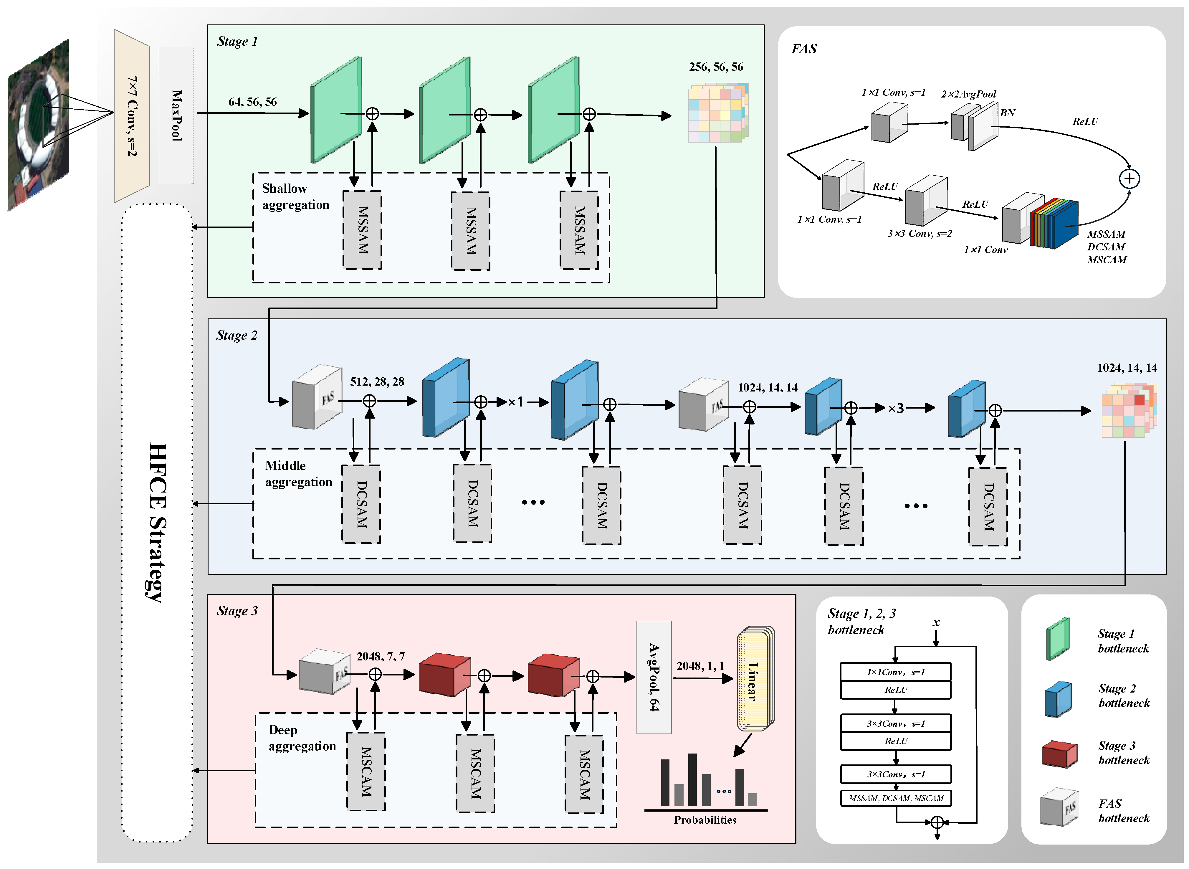
The framework of the network shown in Figure 1 consists of a $7\times 7$ convolution with stride of 2, a down-sampling max pooling, three sets of feature extraction bottleneck modules—stages 1 to 3—and the linear layer. Specifically, stage 1 comprises three no-down-sampling bottlenecks, each incorporating a lightweight MSSAM. Similarly, stage 2, corresponding to the middle layers of the ResNet50, embeds the lightweight DCSAM. At this stage, two featured average sampling (FAS) bottlenecks are used for down sampling. After the first down sampling, the spatial dimensions (height and width) of the feature maps are halved and the channel count is doubled, followed by three bottlenecks. After the second down sampling, another five bottlenecks are appended, further halving the spatial dimensions and doubling the channel count once again. In stage 3, an FAS bottleneck first performs down sampling, followed by two bottlenecks. All the bottlenecks in this stage are incorporated with a lightweight MSCAM. The resulting feature map is then average-pooled and passed through linear layers to produce the probabilities.

The method for such module arrangement is the HFCE strategy—the shallow layers characterized by high resolution and massive spatial information employ lightweight MSSAM for preliminary extraction of multiscale spatial features; deeper layers, with more channels and broader receptive fields, concentrate on channel feature extraction; the middle layers focus on extracting the co-relationship between channels and spatial information. The integration of attention modules across layers, combined with the lightweight processing of these mechanisms, elevates efficient feature extraction while maintaining the network’s parameter scale of 29.0 M with 1000 classes.

The modified residual block structure is shown in the upper right corner of Figure 1. By setting the stride of the $1\times 1$ shortcut convolutional kernel to 1, and cascading an average pooling layer with a stride of 2 and a kernel size of $2\times 2$ after this convolutional layer to achieve down sampling, the dimensionality of the feature map is effectively reduced while avoiding the omission of features. This is achieved without introducing additional learnable parameters. Additionally, the abovementioned attention module that maintains the same input and output size is embedded after the third $1\times 1$ convolutional kernel in the main path. Note that after their feature map generation differs, all three operate on the output of the third convolution in the main path; MSSAM and MSCAM produce attention weights that are multiplied element-wise with the input feature map, whereas DCSAM generates feature maps that are added element-wise to the input feature map. In every case, the result is then summed element-wise with the shortcut branch.

2.2. HFAE Strategy

In this paper, the proposed hierarchical attention enhancing mechanism embeds different attention modules at various levels of the residual network, constructing an improved feature extraction architecture. This approach effectively enhances the network’s capability to represent multi-dimensional features of remote sensing objects while optimizing computational effectiveness. We introduce three enhanced lightweight multiscale attention modules, all designed with input dimensions matching the output dimensions. This dimensional invariance allows for seamless integration into the network. Below, we present the mathematical formulations for generating feature information in each attention module.

2.2.1. MSSAM

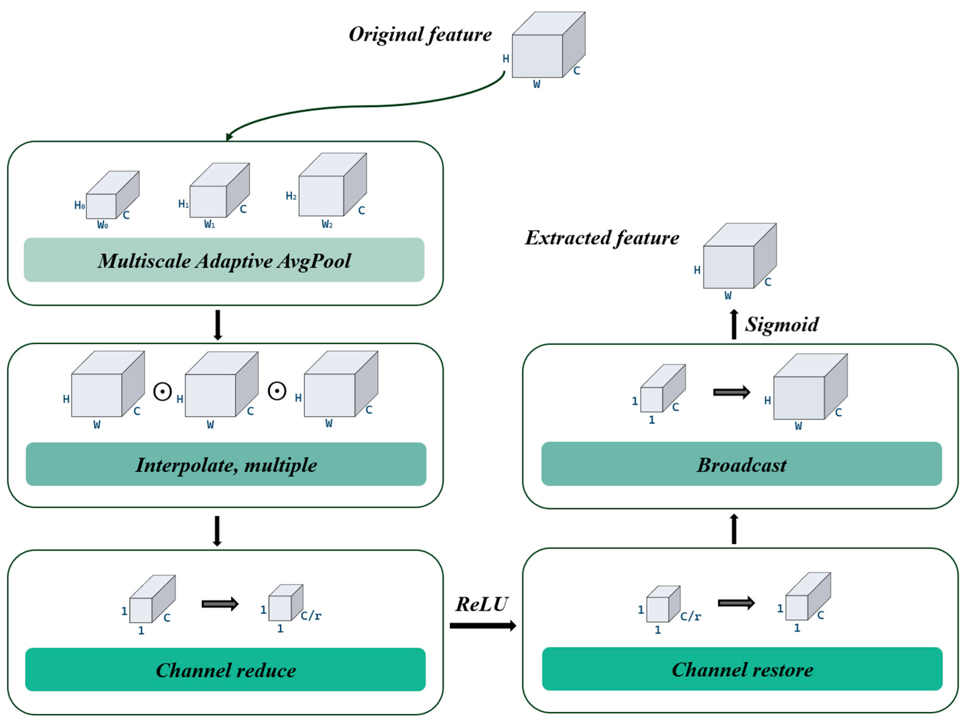
Stage 1 of the backbone network integrates the lightweight MSSAM into the bottleneck. With the aim of reducing model parameters, it preliminarily enhances feature fusing through multiscale spatial extraction, shown in Figure 2.

Firstly, the module performs a multiscale fusion operation on the input image, employing feature extraction with different kernel sizes. In this approach, three adaptive average pooling layers of different sizes are defined, respectively, as $1\times 1$, $2\times 2$ and $3\times 3$. These pooling methods with different kernel sizes are conducive to enhancing the network’s generalization and sensitivity to features of varying scales. After performing multiscale pooling operations on the input image, the resulting feature maps are resized to their original dimensions using bilinear interpolation. The three pooled feature maps are then linearly combined and multiplied element-wise with the original features, thereby achieving the fusion and enhancement of cross-scale local feature responses. Here, the formula is defined as

$$F_{fused}=F⨀\underset{s\in \left\{\mathrm{1,2},3\right\}}{\sum Itp({AvgPool}_s(F)})$$

(1)

where $F_{fused}$ represents fused feature tensor, $F$ is the tensor before fusing, $Itp$ is the bilinear interpolation function and ${AvgPool}_s$ represents an adaptive pooling function with size $s$.

Let the original input be the four-dimension tensor $X\in {\mathbb{R}}^{B\times C\times H\times W}$. Then it undergoes global average pooling $AvgPool$ after feature fusion to the size of $\left[B,C,1,1\right]$; the formula is defined as

$$z_c={\displaystyle \frac{1}{H\times W}}{\sum }_{i=1}^H{\sum }_{j=1}^W{X}_c\left(i,j\right)$$

(2)

Here, $X_c$ is the input feature, $B$ is the training batch, $C$ is the channel account, $H$ and $W$ are the height and weight of the input, and $z_c$ is the global average of one channel. Then, we send features to the first convolutional layer and reduce the dimensions, which helps to decrease the computational complexity. The second convolutional layer will receive the results after activation function processing, restoring the dimensions to their initial values and performing output after being activated. The whole process including average pooling can be described via

$$F_{sa}=\sigma \left(W_2\cdot GELU\left(W_1\cdot AvgPool\left(F_{fused}\right)\right)\right)$$

(3)

Here, $W_1\in {\mathbb{R}}^{\left(C/r_0\right)\times C\times 1\times 1}$ and $W_2\in {\mathbb{R}}^{C\times \left(C/r_0\right)\times 1\times 1}$ are the tensors for channel reduction and restoration, where the compression ratio can be set to 2, 4, 8, 16 and 32. $GELU$ as the Gaussian Error Linear unit and $\mathsf{\sigma }$ as the sigmoid are different activation functions which will be illustrated in the following context.

Finally, after broadcasting to initial size, the obtained feature $F_{sa}$ is summarized with the original feature. We define $F_{out}=F_{sa}\times F$. This module contributes to the spatial integrity of rudimentary visual features such as edges and textures at a minimal computational cost in shallow networks, providing richer primary spatial feature inputs for deeper networks.

2.2.2. DCSAM

In the backbone network, the bottleneck blocks of stage 2 in the middle network are strengthened by embedding the DCSAM. The DCSAM consists of two components: the coordinate attention module and the regional spatial attention module. These components are designed to capture feature information from channels and spatial dimensions as well as regions and spatial dimensions, respectively, and then integrate this information. The structure is shown in Figure 3.

The coordinate attention module (left) performs adaptive average pooling along the horizontal and vertical directions separately. Assuming the original feature tensor is $X\in {\mathbb{R}}^{B\times C\times H\times W}$, average pooling is conducted based on height and width respectively with the function $Pool$. The pooling formulas are

$${Pool}_h\left(F\left(c,i\right)\right)={\displaystyle \frac{1}{W}}{\sum }_{j=1}^{W}F\left(c,i,j\right)$$

(4)

$${Pool}_w\left(F\left(c,j\right)\right)={\displaystyle \frac{1}{H}}{\sum }_{i=1}^{H}F\left(c,i,j\right)$$

(5)

The resulting features are $X_h\in {\mathbb{R}}^{B\times C\times H\times 1}$ and $X_w\in {\mathbb{R}}^{B\times C\times 1\times W}$. These tensors are concatenated along the second dimension forming a tensor of shape $\left[B,C,H+W,1\right]$. The average pooling is performed to summarize the overall features of each dimension. After concatenation, the channel means and the height and width averages are highly correlated, thereby capturing spatial dependencies. The formula is defined as

$$X_h={Pool}_h\left(F\right),X_w={Pool}_w\left(F\right)$$

(6)

$$Y=Concat(X_h,X_w)\in {\mathbb{R}}^{B\times C\times (H+W)\times 1}$$

(7)

Here, $Concat$ is the concatenation function.

The resulting feature tensors go through channel reduction operation. After passing through a $1\times 1$ convolution which reduces the channel to $C∕r_1$ and an activation function, it generates channel attention weights in both row and column directions, where the compression ratio $r_1$ can be set to 2, 4, 8, 16, 32 and 64. Here, $BN$ is BN and $Hard-swish$ is an activation function which will be illustrated in the following paper.

$$Y=Hard-swish\left(BN\left({Conv}_1\left(Y\right)\right)\right)\in {\mathbb{R}}^{B\times \left(C∕r\right)\times (H+W)\times 1}$$

(8)

After that, the feature tensor is split back to the original size to obtain $Y_h\in {\mathbb{R}}^{B\times \left(C/r\right)\times H\times 1}$ and $Y_w\in {\mathbb{R}}^{B\times (C∕r)\times 1\times W}$. Finally, the number of channels is restored, where $W\in {\mathbb{R}}^{C\times (C∕r)\times 1\times 1}$. The multiply operation is performed after $A_h$ and $A_w$ are broadcasted to initial size. The process can be demonstrated via

$$A_h=\sigma \left(W·Y_h\right)\in {\mathbb{R}}^{B\times C\times H\times 1},A_w=\sigma \left(W·Y_w\right)\in {\mathbb{R}}^{B\times C\times 1\times H}$$

(9)

$$X_{ca}=X⨀A_h⨀A_w\in {\mathbb{R}}^{B\times C\times H\times W}$$

(10)

Regional spatial attention (right) performs average and maximum pooling on the channel dimension and concatenates the results. The key point is that it divides the feature map into local blocks using a regional partitioning strategy. It then applies a $7\times 7$ convolutional kernel to each block to generate spatial attention weights. After concatenation, the global size is restored, thus achieving fine-grained feature focusing in local regions. The entire process can be demonstrated via

$$X_{sa}\left(F\right)=X⨀\sigma {⨁}_i^n{Conv}_7\left({Region}_i\left(Concat\left(AvgPool\left(F\right),MaxPool\left(F\right)\right)\right)\right)\in {\mathbb{R}}^{B\times C\times H\times W}$$

(11)

Here, $MaxPool$ is the maximum pooling operation while ${Conv}_7$ is the $7\times 7$ convolution operation and ${⨁}_i^n$ is the joint function on the fourth dimension. So far, the feature tensor obtained in this paper has the same size as the original input feature tensor. Therefore, a fusion mechanism is adopted to dynamically balance the contributions of channel and spatial attention using learnable parameters $\alpha$ and $\beta$. This is combined with residual connections to achieve multi-dimensional feature enhancement. If the residual part is included, the following formula can be defined as

$$F_{out}=\alpha \cdot X_{ca}+\beta \cdot X_{sa}+\mathrm{X}$$

(12)

This design establishes complementary enhancement between cross-channel long-range dependencies and local spatial details in the mid-level features. It effectively improves the feature discrimination ability of medium-scale objects such as buildings and roads in images.

2.2.3. MSCAM

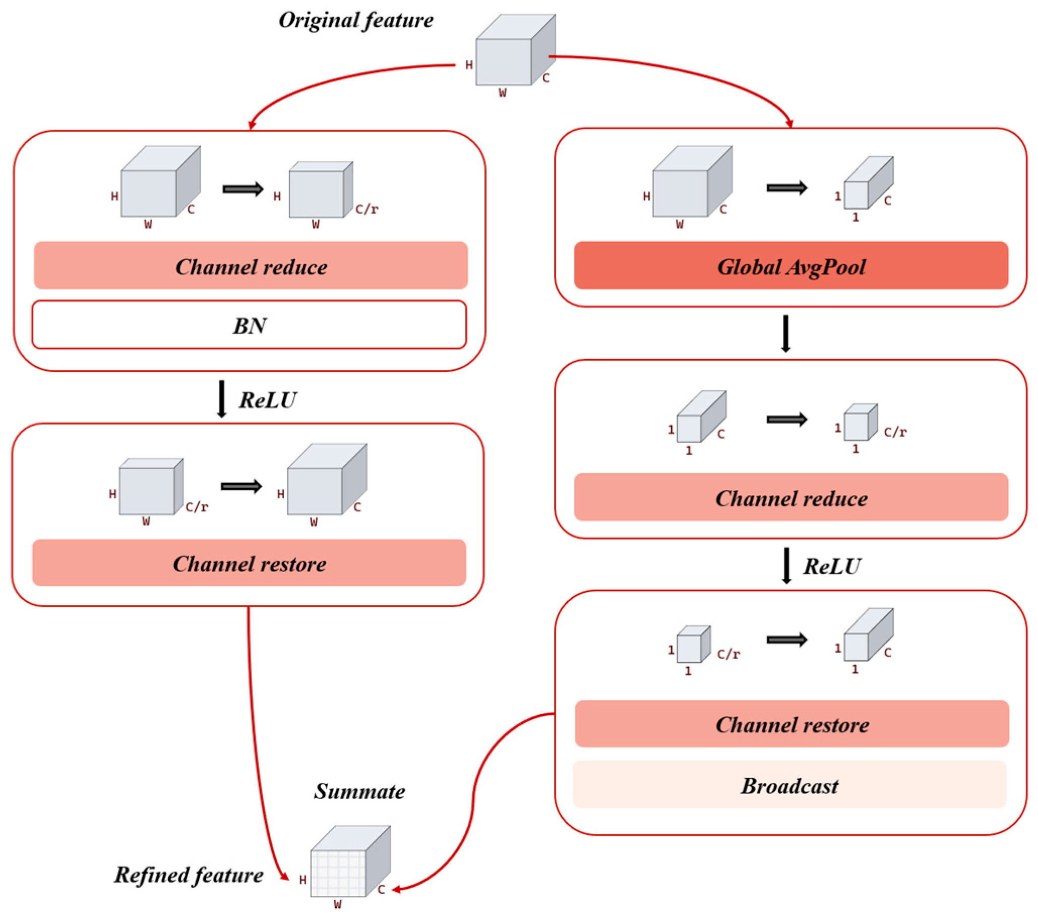
To establish cross-channel multiscale dependencies in the mid-to-deep layer features, the bottlenecks of stage 3 in the original network employ a lightweight MSCAM, whose structure is shown in Figure 4. The module achieves adaptive recalibration of channel features through parallel local and global channel attention mechanisms while maintaining computational efficiency. This significantly enhances its ability to fuse multiscale information.

The module receives an input tensor of size $[B,C,H,W]$. The intermediate number of channels $C_0$ is calculated as $C_0=C/r_2$ where the compression ratio can be set to 2, 4, 8, 16, 32 64 and 128. Subsequently, channel attention is extracted through two parallel branches.

Firstly, local attention (left) is achieved through dimensionality reduction convolution, BN, and activation functions to implement pixel-wise local channel interaction, enhancing the channel dependency of spatially local features.

$$X_{local}=W_2^{loc}(\sigma \left(BN\right(W_1^{loc}\left(X\right)\left)\right)$$

(13)

Here, $W_1^{loc}\in R^{C\times C_0\times 1\times 1}$ and $W_2^{loc}\in R^{C_0\times C\times 1\times 1}$ are respectively local channel reduction and restoration convolution operation, and $BN$ is BN. $\sigma$ is a Rectified Linear Unit (ReLU). This branch enhances the channel dependency of spatial local features through pixel-wise local channel interaction.

Global attention uses global average pooling to compress feature maps into global statistics. After processing through channel reduction convolution, activation functions, and channel restoration convolution, it models long-range dependencies across channels. The computation can be expressed as follows:

$$X_{global}=W_2^{glo}(\sigma \left(W_1^{glo}\right(GAP\left(X\right)\left)\right)$$

(14)

where $GAP$ represents adaptively global average pooling to $1\times 1$ while $W_1^{glo}\in R^{C\times C_0\times 1\times 1}$ and $W_2^{glo}\in R^{C_0\times C\times 1\times 1}$ are two global channel reduction and restoration convolution operations. The obtained feature $X_{global}$ is broadcasted to initial size.

Fusion of the global and local features is achieved through element-wise addition, and a channel weight map is generated through the sigmoid activation function: $A =Sigmoid(X_{local}+X_{global})\in {\mathbb{R}}^{B\times C\times H\times W}$. Then the output feature is calculated as

$$F_{out}=X⨀A$$

(15)

This design establishes a complementary enhancement mechanism for local and global channel dependencies during deep feature processing, introducing only about 1.8 K learnable parameters.

2.3. Structure of FAS Bottleneck

In the common residual network architecture, the down-sampling operation of the shortcut connection (SC) is typically accomplished by a convolutional kernel with a size of $1\times 1$ and a stride of 2. This operation reduces the size of the input feature map $X_{in}\in {\mathbb{R}}^{B\times C\times H\times W}$, and the convolutional kernel extracts features in a skip-sampling manner, causing some pixel information to be directly discarded and unable to participate in subsequent feature representation. To address this, an improved solution is proposed: the stride of the original convolutional kernel is changed from 2 to 1, allowing the kernel to slide pixel by pixel and fully traverse every position of the input feature map. This approach thoroughly extracts local detail features and prevents omission of important information. To achieve the effect of down sampling, an average pooling layer with a size of $2\times 2$ and a stride of 2 is added after the SC convolutional kernel. This allows for an effective reduction in the size of the feature map without introducing additional learnable parameters.

The improved structure proposed in this paper involves two consecutive operations: full-sampling convolution

$$X_{conv}={Conv}_{1\times 1}^{stride=1}\left(X_{in}\right),X_{conv}\in R^{B\times C^{\prime }\times H\times W}$$

(16)

and adaptive down sampling

$${\mathrm{X}}_{\mathrm{o}\mathrm{u}\mathrm{t}}={\mathrm{A}\mathrm{v}\mathrm{g}\mathrm{P}\mathrm{o}\mathrm{o}\mathrm{l}}_{2\times 2}^{\mathrm{s}\mathrm{t}\mathrm{r}\mathrm{i}\mathrm{d}\mathrm{e}=2}\left({\mathrm{X}}_{\mathrm{c}\mathrm{o}\mathrm{n}\mathrm{v}}\right),{\mathrm{X}}_{\mathrm{o}\mathrm{u}\mathrm{t}}\in {\mathrm{R}}^{B\times {\mathrm{C}}^{\prime }\times H∕2\times W∕2}$$

(17)

Compared to the rudimentary structure, the improvements proposed in this paper have the following significant advantages: (1) The convolutional kernels extract features pixel by pixel, which fully preserves the fine-grained structures and small target features in remote sensing images, enhancing the sensitivity to details. (2) Average pooling integrates features through local mean values, which helps to alleviate abrupt changes in features and enhances the network’s robustness and generalization capability. (3) It avoids introducing additional convolutional parameters, ensuring the overall computational overhead and inference speed of the network.

2.4. Advanced Network Nonlinearity Mechanism

In CNNs, to overcome such issues of the loss of propagation capability of ReLU activation function caused by a gradient of zero with the negative half-axis, known as “neuron death”, this model employs the GELU activation function in the MSSAM. GELU is a self-regularizing activation function that probabilistically sets the input to zero based on the Gaussian Distribution of the inputs. It is also smoother around the origin than ReLU. The formula is

$$GELU\left(x\right)=x\Phi \left(x\right)$$

(18)

Here, $\mathsf{\Phi }\left(\mathrm{x}\right)$ is the cumulative distribution function of the Standard Normal Distribution. Taking the derivative of GELU, according to the product rule of differentiation, we have

$${\mathrm{GELU}}^{\prime }\left(x\right)=\Phi \left(x\right)+x\phi \left(x\right)$$

(19)

Additionally, in the DCSAM, the Hard-swish activation function is also used regarding the design of the nonlinear unit, which helps extract more rich details and features which have high similarity in the middle layers of the network [3]. The formula is

$$ReLU6\left(x\right)=min\left(max\right(0,x),6)$$

(20)

$$Hard-swish(x)=x\cdot {\displaystyle \frac{ReLU6(x+3)}{6}}$$

(21)

Finally in terms of regularization strategies, the network introduces L2 regularization to achieve dual optimization objectives of suppressing overfitting through weight decay and enhance expressing key features.

$$J(\Theta )={\displaystyle \frac{1}{2m}}[{\sum }_{i=1}^m(v\Theta (x_i)-y_i{)}^2+\lambda {\sum }_{j=1}^n{\Theta }_j^2]$$

(22)

Here, the regularization coefficient $\lambda$ determined through grid search is set to 0.005.

3. Experiment and Analysis

This section describes the experiment materials, settings, details and analysis based on our proposed network. The model is trained on four standard remote sensing scene image datasets and estimated through overall accuracy (OA), Kappa coefficient, average precision (AP) and F1 score. At the same time, confusion matrixes (CMs) are adopted to illustrate models’ classifying performance which can be estimated visually.

3.1. Datasets

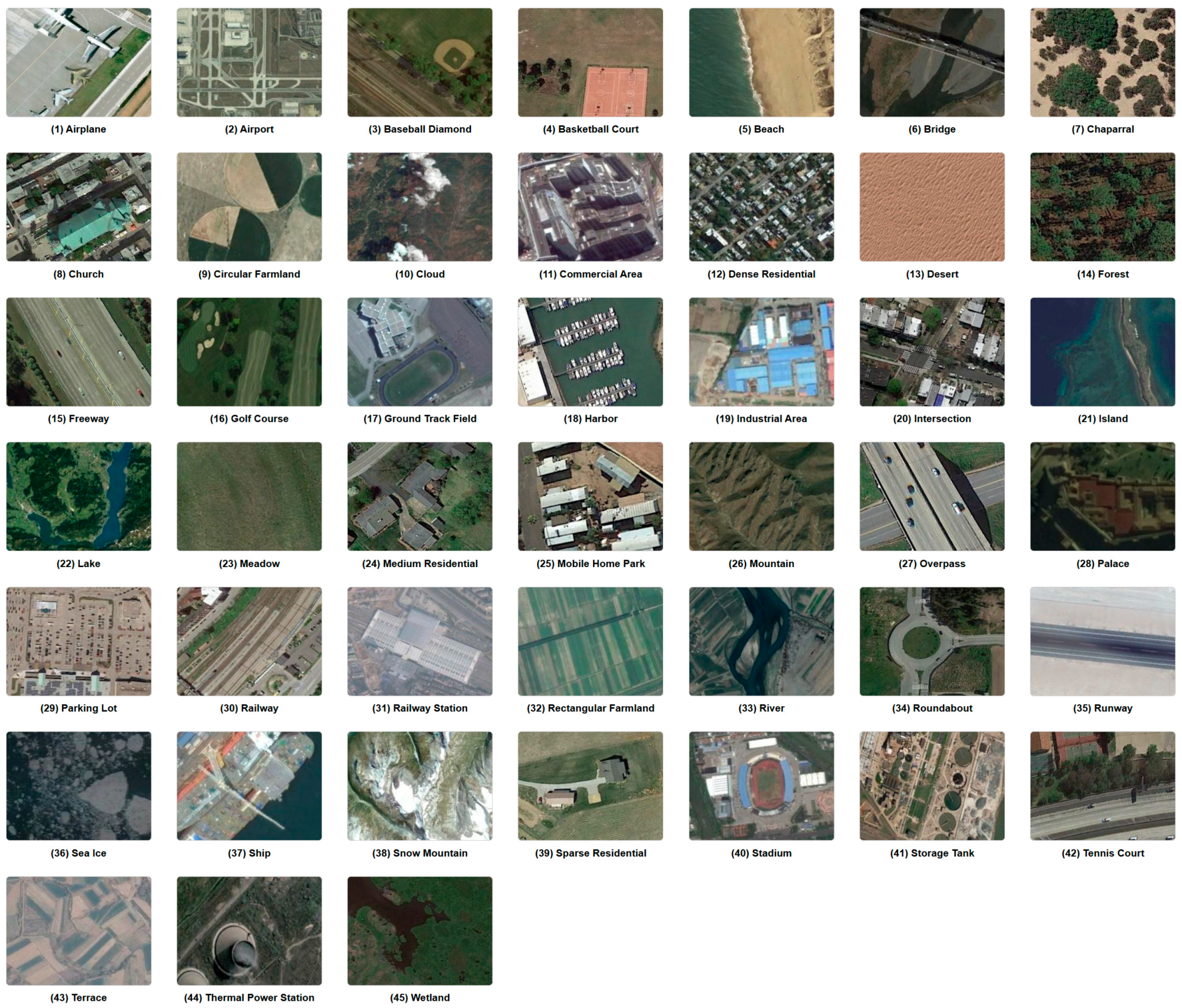
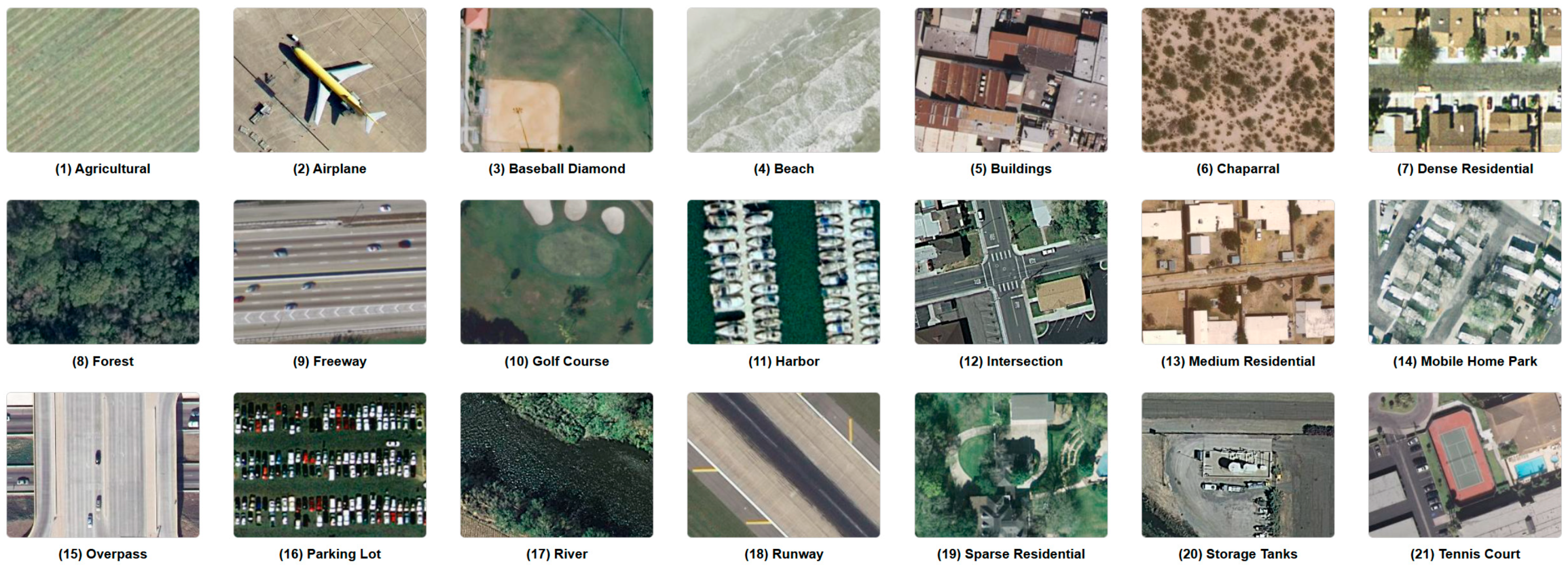
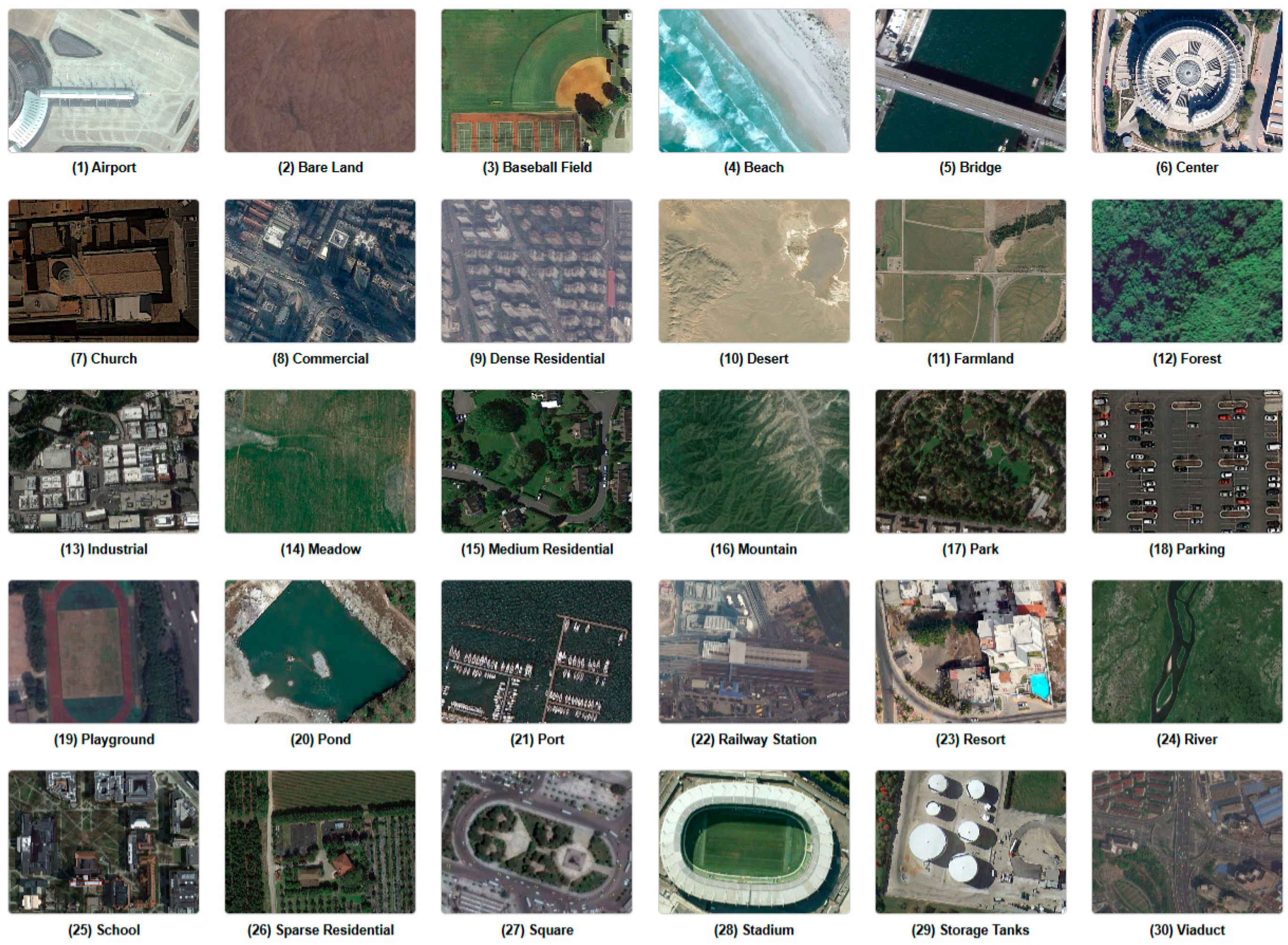
In this part, we introduce four standard datasets for remote sensing scene image classification, namely RSSCN7, NWPU45, UCM21, AID30. Figure 5, Figure 6, Figure 7 and Figure 8 show some examples of the four datasets.

3.1.1. RSSCN7

As a typical dataset for multiscale remote sensing scene analysis, the RSSCN7 dataset was constructed in 2015. It fuses data from Google Earth images, covering 7 major categories (grassland, forest, farmland, parking lots, residential areas, industrial areas, rivers) and 28 subcategories. The dataset comprises 2800 radiometrically corrected image samples, each standardized to 400 × 400 pixels and using the UTM projection coordinate system. This dataset offers two key advantages: (1) a multi-resolution hierarchical structure, where each scene category includes four spatial scales ranging from local textures to global layouts, and (2) cross-seasonal variation modeling, with 30% of samples showing significant seasonal features. Some samples are shown in Figure 5.

3.1.2. NWPU45

The NWPU45 dataset, one of the most widely globally covered public benchmark datasets for remote sensing, is specifically dedicated to remote sensing image scene classification tasks. The dataset acquires original images through collaborative collection via satellite platforms, aerial photography, and GIS data fusion. It covers 102 typical regions across six continents with a longitude range from −170° to 175° and latitude range from −55° to 78°, and each region has a collection radius of ≥50 km. Spanning from 2015 to 2022, it includes seasonal periodic sampling with at least 50 samples per quarter. The dataset contains 45 categories, with 700 images per category. The images are 256 × 256 pixels in size, with a resolution ranging from 0.2 to 30 m. Some samples are shown in Figure 6.

3.1.3. UCM21

As a benchmark dataset for urban remote sensing research, the UCM21 dataset was first proposed in 2010, with data sourced from the national map of the Urban Area Imagery program of the United States Geological Survey (USGS). The dataset systematically collects 21 categories of typical urban land use scenes, each containing 100 strictly geometrically corrected RGB images, totaling 2100 samples. The original images are standardized to 256 × 256 pixels, with a spatial resolution of 0.3 m and a color depth of 8 bits per channel. Notably, the intra-class difference between the “dense residential” and “medium-density residential” categories reaches 12.7%, making it an effective benchmark for evaluating the fine-grained recognition capability of models.

3.1.4. AID30

AID30, a benchmark in high-resolution remote sensing image scene classification, has served as a crucial experimental platform for remote sensing intelligent interpretation research since it was first proposed by the Wuhan University team in 2017. It adheres to the geographic space sampling theory and employs a stratified random sampling strategy. The dataset’s imagery primarily originates from multi-temporal satellite images of the Google Earth platform (2013–2016), forming a collaborative construction model of multisource heterogeneous data. It covers typical regions of different climate zones and geographic features worldwide, including urban–rural areas and agricultural, industrial, and natural landform types. Spanning major continents such as Asia, Europe, and North America, it encompasses 30 scene categories with significant semantic differences, each containing approximately 220–420 images, totaling about 10,000 samples. The images are standardized to 600 × 600 pixels with a spatial resolution ranging from 0.5 to 8 m, enabling clear representation of ground object details. Notably, the dataset demonstrates remarkable advantages in scene diversity, inter-class distinguishability, and intra-class variability.

3.2. Experiment Setup

In image preprocessing, scale all input images to 224 × 224 pixels. Apply random cropping with an area ratio between 80% and 100% of the original image, and perform horizontal flipping with a 50% probability; then, randomly rotate images within ±30 degrees, and adjust brightness, contrast, and saturation with random variations of ±20%. Finally, images are normalized. In terms of hyperparameters, the optimizer selected is the stochastic gradient descent (SGD), with the maximum learning rate set to 0.005 and learning rate scheduler set to 0.2, indicating that it will increase from the initial value of 0.0005 to the maximum value within the first 20% of epochs. The compression ratio $r_0$ for MSSAM is set to 16, $r_1$ for DCSAM is set to 32 and $r_2$ for MSCAM is set to 16. The coefficient $\lambda$ for L2 regularization is set to 0.005. A cosine annealing strategy was used during training. The models were trained for 200 epochs with batch size of 64, on devices equipped with an Intel (R) Core (TM) i9-14900HX 2.20 GHz CPU (Intel Corporation, Santa Clara, CA, USA), NVIDIA RTX 4060 GPU (NVIDIA Corporation, Santa Clara, CA, USA), and 16.0 GB of onboard RAM (Micron Technology, Inc., Boise, ID, USA). To avoid experimental errors caused by uncertain issues, each experiment is set to repeat 10 times and the standard deviations are recorded.

3.3. Performance of the Proposed Method

The network proposed in this study is an improvement over the ResNet50 network. To verify the effectiveness of the proposed network, a comparison with ResNet50 is first performed on the UCM21 dataset. OA, KAPPA, AP and F1 are used as the evaluation metrics. The experiment uses a pre-trained original ResNet50 for reproduction.

Table 1. OA performance comparison between original and proposed model. The notation a/b dataset denotes the data split ratio, where a% of the data is used for training and b% for testing.

Dataset	ResNet50				HLAE-Net (Ours)
	OA (%)	KAPPA (%)	AP (%)	F1	OA (%)	KAPPA (%)	AP (%)	F1
50/50 UCM21	98.19	98.10	98.26	98.19	98.76	98.70	98.80	98.76
80/20 UCM21	99.53	99.55	99.50	99.52	99.77	99.77	99.75	99.76
20/80 AID30	93.91	93.81	93.71	93.51	94.26	94.03	94.10	93.85
50/50 AID30	96.32	96.19	96.21	96.07	96.50	96.38	96.39	96.30
80/20 RSSCN7	96.43	95.86	96.51	96.41	97.14	96.68	97.22	97.14
10/90 NWPU45	90.84	91.06	90.65	90.85	91.88	91.93	91.71	91.84
20/80 NWPU45	93.41	93.45	93.27	93.39	94.01	93.88	94.04	94.00

presents a comparison of the arithmetic mean OAs between the trained model in this paper and the ResNet50 model.

From Table 1, it can be observed that the performance of the proposed methods is better than ResNet50. On the NWPU45 dataset, with a 10% training ratio, the proposed model outperforms the ResNet50 model by 1.02% in OA, 0.87% in KAPPA, 1.06% in average precision (AP), and 0.99% in F1 score, making it one of the datasets where the proposed model performs particularly well. Additionally, on the RSSCN7 dataset, with a training ratio of 10%, the proposed model surpasses the original model by 0.64% in OA, 0.65% in KAPPA, 0.74% in AP, and 0.64% in F1 score, which is relatively a better-performing dataset. Furthermore, on other datasets, the model also demonstrates improvements in recognition performance to varying degrees.

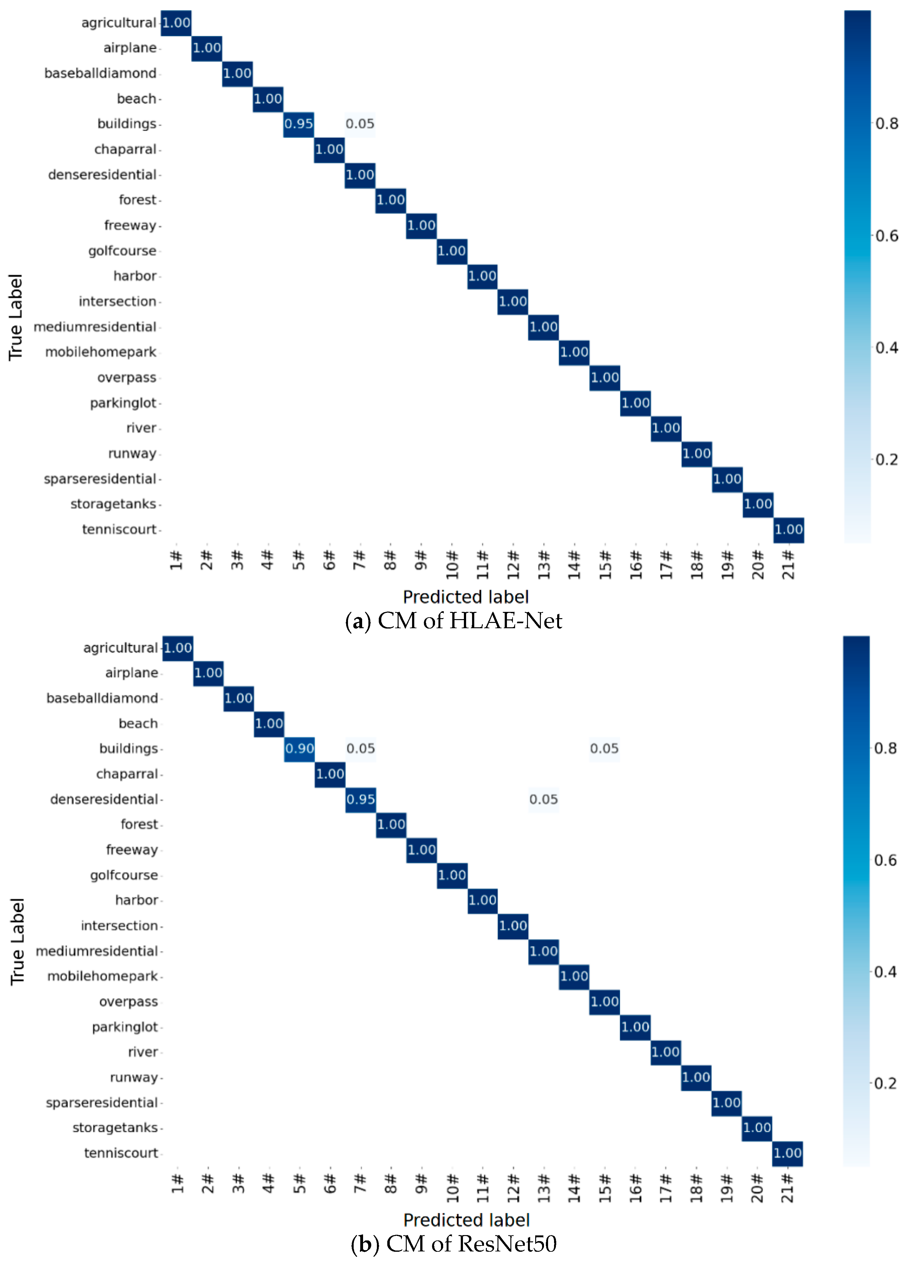
On the UCM21 dataset, ResNet50 has already achieved good performance, with a mean OA as high as 98.19% with a 20% training ratio and 99.53% with an 80% training ratio. However, the proposed model has further enhanced all four metrics on this basis, increasing the mean OA to 98.81% and 99.76%, respectively. The KAPPA has been improved to 98.70% and 99.77%, the AP to 98.80% and 99.75%, and the F1 score to 98.76% and 99.76%. The CMs are shown in Figure 9. The proposed model performs well in recognizing all categories except for buildings, with either all correct identifications or an error rate less than 0.05, while the original model makes more mistakes.

3.4. Ablation Study

This section will test the validity of the proposed module. For the proposed MSSAM, DSCAM and MSCAM modules, we adopted a pin-two combination to join the network and conducted FAS optimization (Case 2–4), using the original network (Case 1) as the baseline comparison experiment. For the FAS bottleneck, the original down-sampling network with the addition of the complete attention module group (Case 5) was used as the baseline comparison experiment. All experiments were conducted on four datasets, and a small training ratio with better model gain was adopted. As we can see from

Table 2. Ablation experiments. (OA and standard deviation are adopted as the evaluation indicators. The notation a/b dataset denotes the data split ratio, where a% of the data is used for training and b% for testing.)

Case	Components				Datasets
	MSSAM	DCSAM	MSCAM	FAS	50/50 UCM21	10/90 NWPU45	80/20 RSSCN7	20/80 AID30
1	✗	✗	✗	✗	98.19 ± 0.11	90.84 ± 0.12	96.43 ± 0.22	93.91 ± 0.23
2	✓	✓	✗	✓	98.46 ± 0.13	91.55 ± 0.19	96.82 ± 0.32	94.15 ± 0.14
3	✓	✗	✓	✓	98.36 ± 0.18	91.44 ± 0.20	96.61 ± 0.12	94.14 ± 0.20
4	✗	✓	✓	✓	98.42 ± 0.11	91.43 ± 0.08	96.71 ± 0.13	94.18 ± 0.20
5	✓	✓	✓	✗	98.65 ± 0.23	91.70 ± 0.12	97.04 ± 0.09	94.24 ± 0.09
6	✓	✓	✓	✓	98.76 ± 0.13	91.88 ± 0.19	97.14 ± 0.14	94.26 ± 0.26

, compared with Case 1, the OAs of Cases 2–4 increased by 0.17–0.27% on UCM21, by 0.59–0.71% on NWPU45, by 0.18–0.39% on RSSCN7 and by 0.23–0.27% on AID30%. When three modules are added simultaneously without FAS optimization (Case 5), the OAs improve 0.46%, 0.86%, 0.61% and 0.33% respectively. It can be seen that the proposed modules can enhance network performance, and when the three work together, the performance can be further improved. For Case 6, the model gains further improve to 0.57%, 1.04%, 0.71% and 0.35% respectively. This result confirmed the validity of the FAS bottleneck.

3.5. Comparisons with Some State-of-the-Art Methods

To comprehensively evaluate the classification performance of the proposed model, we compared our method with some state-of-the-art methods. These include ResNet50-EAM, ACR-MLFF, SAFF, GBNet, PVT-v2_B0, SCCov, D-CapsNet, lv-vit-s, APDC-Net, LCNN-BFF, TAKD, EMTCAL, HFAM, ViT, GLR-CNN, SPTA, T-CNN, ACnet, AG-MANet-Split, GCSANeT, MogaNet, EfficientNetV2, EfficientNetB3-Attn-2, L2RCF, and RSSCNet. Please note that the results of the methods used for comparison in the text are from the original literature, and except for image size, other experimental settings are the same as ours.

3.5.1. Experiment on UCM21

The UCM21 dataset is a dataset with relatively low recognition difficulty and is widely used, offering many comparable methods. We conducted experiments with the proposed model by setting the training set proportion to 80%, and the results are shown in

Table 3. OAs and standard deviations of the proposed model and some state-of-the-art models on UCM21.

Methods	Year	80% Training
D-CapsNet [22]	2019	99.05 ± 0.12
SCCov [23]	2019	99.05 ± 0.25
PVT-v2_B0 [24]	2020	98.86 ± 0.38
APDC-Net [25]	2020	97.05 ± 0.43
LCNN-BFF [26]	2020	99.29 ± 0.24
ViT [27]	2021	99.29 ± 0.21
lv-vit-s [28]	2021	99.28 ± 0.16
EMTC AL [16]	2022	99.58 ± 0.32
TAKD [29]	2024	97.33 ± 0.25
GLR-CNN [27]	2024	99.14 ± 0.26
HFAM [14]	2024	98.67 ± 0.21
HLAE-Net (ours)	2025	99.77 ± 0.00

. It can be seen that PVT-v2_B0 and lv-vit-s did not perform as well as several other methods. In comparison, SCCov increased the average recognition accuracy to 99.05%, with a parameter size of 25.1 M. D-CapsNet improves the dynamic routing mechanism of the traditional capsule network (CapsNet) and the model performs well on tasks such as fine-grained classification, pose estimation, and few-sample learning. Its mean value on the dataset is the same as SCCov’s, but it has a smaller variance. For the other two models, lv-vit-s and LCNN-BFF, the proposed model in this paper further improves the recognition accuracy by 0.5% on the basis of their performance. Compared to EMTCAL, which shows a relatively good performance, this model has an OA mean value that is 0.19% higher. In addition to these, this model, after several training sessions, achieves a variance of near-zero on the UCM21 dataset, demonstrating stability. The CMs are shown in Figure 9.

3.5.2. Experiment on NWPU45

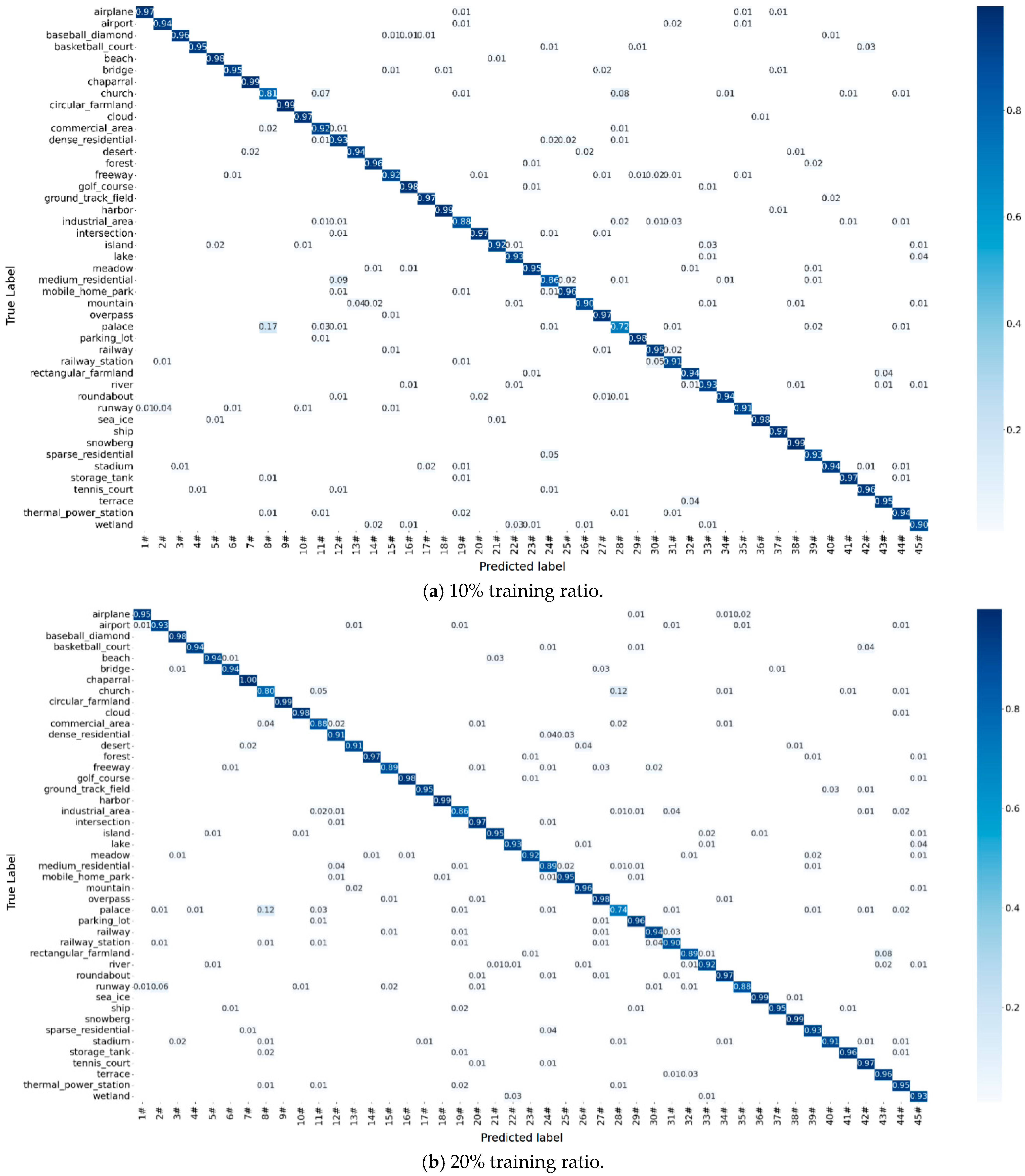
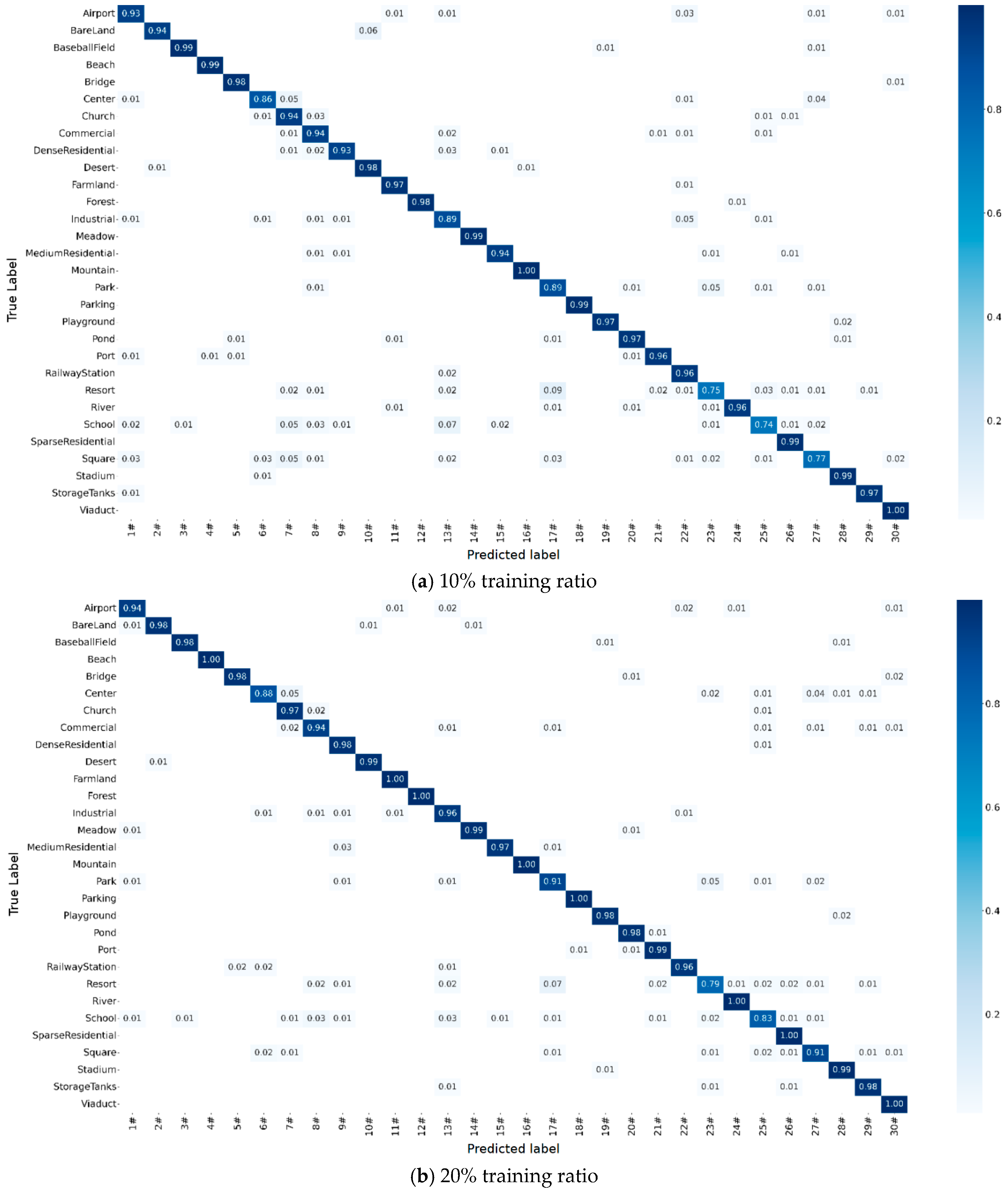
The NWPU45 dataset is the largest dataset used in the experiment, covering the broadest range and featuring the most complex classification, making it relatively challenging to learn. In the experiment, training ratios of 10% and 20% were set to test the model’s ability to learn with a small amount of data on a large and challenging dataset. The CMs can be seen in Figure 10. From

Table 4. OAs and standard deviations of the proposed model and some state-of-the-art models on NWPU45 dataset.

Methods	Year	10% Training	20% Training
GBNet [30]	2019	90.49 ± 0.17	93.33 ± 0.21
D-CapsNet [22]	2019	88.18 ± 0.19	92.46 ± 0.14
ResNet50-EAM [31]	2020	90.89 ± 0.15	93.51 ± 0.12
SAFF [32]	2020	84.38 ± 0.19	87.86 ± 0.14
PVT-v2_B0 [24]	2020	89.72 ± 0.16	92.95 ± 0.09
SCCov [23]	2020	89.30 ± 0.35	92.10 ± 0.25
APDC-Net [25]	2020	85.94 ± 0.22	87.84 ± 0.26
LCNN-BFF [26]	2020	86.53 ± 0.15	91.73 ± 0.17
lv-vit-s [28]	2021	91.60 ± 0.12	93.48 ± 0.15
ViT [27]	2021	91.58 ± 0.19	93.90 ± 0.20
ACNet [33]	2021	91.09 ± 0.13	92.42 ± 0.06
ACR-MLFF [34]	2022	90.01 ± 0.33	92.45 ± 0.20
EMTCAL [16]	2022	91.05 ± 0.17	93.36 ± 0.24
T-CNN [35]	2022	90.35 ± 0.11	93.16 ± 0.17
TAKD [29]	2024	87.96 ± 0.14	91.96 ± 0.16
HFAM [14]	2024	90.81 ± 0.11	-
SPTA [36]	2024	91.74	94.96
HLAE-Net (ours)	2025	91.88 ± 0.19	94.01 ± 0.07

, it can be observed that the proposed model has achieved significant improvements in OA compared to the SAFF and GBNet models, which use VGG as their backbones. With a 10% training ratio, our model achieved an OA that was 6.50% and 1.39% higher than the SAFF and GBNet models, respectively. With 20% of the data used for training, the improvements are 5.74% and 0.29% higher than SAFF and GBNet, respectively. Among them, GBNet’s size is closer to that of our model, with a parameter size of approximately 25.6 M. Compared to the other two methods, ResNet50-EAM and ACR-MLFF, which have approximately 29.0 M and 32.2 M parameters, our model achieved an OA improvement of 0.99% and 1.87% with a 10% training ratio and an improvement of 0.11% and 1.17% with a 20% training ratio. With the 10% training ratio, compared to the remaining networks, the improvements of our model are 3.92% over Tank, 1.07% over HFAM, 0.3% over ViT, 2.53% over GLR-CNN, 0.14% over SPTA, 0.83% over EMTCAL, and 0.79% over ACNet. With the 20% training ratio, the improvements are 2.66% over Tank, 1.51% over GLR-CNN, 0.26% over EMTCAL, 0.46% over T-CNN, and 1.20% over ACNet. It is worth mentioning that at the 20% training ratio, although SPTA shows a slight advantage in OA, this further highlights the superior performance of our method in small-sample learning scenarios (10% training ratio), which are more critical for practical applications, fully demonstrating the effectiveness of the proposed method. In addition, compared with the ViT-based method with a 20% training ratio, the proposed model slightly improved by 0.11% but with a parameter count of only about 0.35 of the former (29 M to 86 M). In conclusion, on the MWPU dataset the proposed model showed improvements compared to other methods, but it also reflects some small improvements in certain circumstances, which is the direction of our future work.

3.5.3. Experiment on RSSCN7

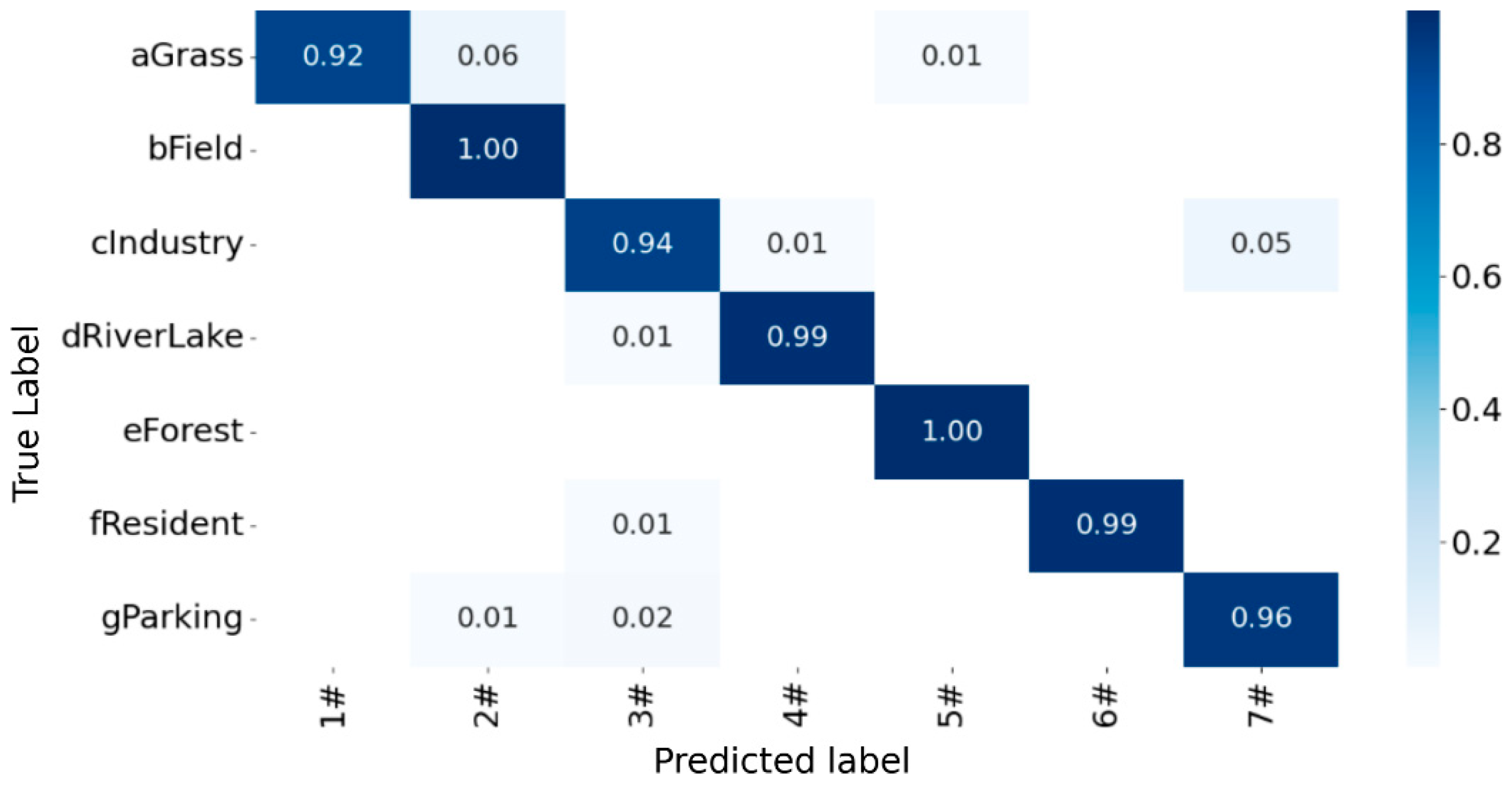
The RSSCN7 dataset has fewer categories, and the proposed model has increased the OA to 97.14%. The CM has been shown in Figure 11. Additionally, compared to other advanced methods according to

Table 5. OAs and standard deviations of the proposed model and some state-of-the-art models on RSSCN7.

Methods	Year	(80% Training)
RSSCNet [37]	2020	97.01 ± 0.21
EfficientNetV2 [38]	2021	95.14 ± 0.21
EfficientNetB3-Attn-2 [39]	2021	96.17 ± 0.16
EMTCAL [16]	2022	93.57 ± 0.25
GCSANet [40]	2022	92.84 ± 0.41
MogaNet [41]	2023	95.14 ± 0.37
LAG-MANet-Split [42]	2023	96.07 ± 0.16
L2RCF [43]	2023	96.05 ± 0.07
HLAE-Net (ours)	2025	97.14 ± 0.14

, it has OA mean improvements of 3.57% over EMTICAL, 1.07% over LAG-MANet-Split, 4.3% over GCSANeT, 2.0% over MogaNet and EfficientNetV2, 0.97% over EfficientNetB3-Attn-2 and 1.09% over L2RCF. It is worth mentioning that it achieves a minor 0.13% improvement over RSSCN7. This is due to the relatively low inter-class similarity of RSSCN7, and still the model delivers a certain improvement for this issue. In future work we will refine the model to further enhance performance on this dataset.

3.5.4. Experiment on AID30

The AID30 dataset is renowned for its extensive climatic variations, land cover, and sampling breadth, posing significant challenges for recognition tasks. The CMs are shown in Figure 12. From

Table 6. OAs and standard deviations of the proposed model and some state-of-the-art models on AID30 dataset.

Methods	Year	20% Training	50% Training
GBNet [30]	2019	92.20 ± 0.23	95.48 ± 0.12
D-CapsNet [22]	2019	92.73 ± 0.15	96.15 ± 0.14
SCCov [23]	2019	93.12 ± 0.25	96.10 ± 0.16
ResNet50-EAM [31]	2020	93.63 ± 0.25	96.62 ± 0.13
SAFF [32]	2020	90.25 ± 0.29	93.83 ± 0.28
PVT-v2_B0 [24]	2020	93.52 ± 0.35	96.27 ± 0.14
APDC-Net [25]	2020	88.56 ± 0.29	92.15 ± 0.29
LCNN-BFF [26]	2020	91.66 ± 0.48	94.62 ± 0.16
lv-vit-s [28]	2021	94.15 ± 0.19	95.66 ± 0.23
ACNet [33]	2021	93.33 ± 0.20	95.58 ± 0.29
ACR-MLFF [34]	2022	92.73 ± 0.12	95.06 ± 0.33
EMTCAL [16]	2022	94.33 ± 0.16	96.12 ± 0.28
TAKD [29]	2024	91.25 ± 0.23	94.80 ± 0.25
HFAM [14]	2024	93.53 ± 0.21	95.94 ± 0.10
GLR-CNN [44]	2024	93.09 ± 0.16	96.49 ± 0.18
SPTA [36]	2024	93.59	96.32
HLAE-Net (ours)	2025	94.26 ± 0.26	96.50 ± 0.25

, it can be observed that compared to the ResNet50-EAM model, the proposed method achieves an OA that is 0.58% higher at the 20% training ratio. Furthermore, among several methods used for comparison, the model has shown improvements under two different splitting methods. Among some methods, it shows improvement by 0.63% over ResNet50-EAM with a 20% training ratio, by 2.06% and 1.01% over GBNet, by 1.14% and 0.40% over SCCov, by 1.53% and 0.35% over D-CapsNet, by 2.60% and 1.88% over LCNN-BFF and by 0.93% and 0.92% over ACNet. Among the most recent models, it has also achieved the best performance at the 50% training ratio, over TAKD by 3.01% and 1.70%, HFAM by 0.73% and 0.56%, GLR-CNN by 1.17% and 0.01%, SPTA by 0.67% and 0.18%, and EMTCAL by 0.38%. For three networks, an inference time experiment under the same condition was conducted by randomly processing 1000 AID30 images 10 times in a loop. The average time is 3.6218 s for ResNet50-EAM, 3.5169 s for HFAM, and 3.5877 s for SPTA, while that of the proposed model is 3.5928 s. The subtle gap reflects the competitiveness of the proposed model. It is also evident that the model performs better with a small training ratio.

4. Discussion

4.1. Model Performance Analysis

The HLAE-Net is proved in experiments to have good performance on the four standard datasets. On the UCM dataset, although the commonly used 50% and 80%training ratios were adopted and the model improvement was nearly saturated, it performed well in both ratios, outperforming some recently proposed and classical networks. On NWPU45, the largest dataset, the model demonstrates advantages in classification, as well as in cases of small training ratios. On RSSCN7, the model also demonstrated better improvement and stronger stability compared to several methods. On the AID30 dataset, the improvement is valid but relatively slight. Compared with other datasets, AID30 uses a much wider range of countries and regions as well as climate and light directions, strengthening the requirement that the model needs to learn more robust features. Meanwhile, its semantic information is more complex. For instance, both bare land and deserts have similar textures and colors, while the former contains artificial traces; both stadiums and playgrounds contain sports fields and the main difference lies in whether there are stands around them. However, it still demonstrates an advantage in the small-training-ratio cases. Therefore, the proposed modules have been found to cooperate effectively, capable of cascading to extract crucial information and avoid less necessary information, thus cumulating the summary of important contextual information in final layers for classification tasks. These attention modules are lightweight, augmenting the learning capability of the entire network while keeping the computational efficiency to extract features. At the same time, the improvements to the bottleneck effectively increase the efficiency of propagation while maintaining the receptive field. The improved network maintains the same order of magnitude of parameters (29 M) as the original network, and its performance surpassed other state-of-the-art methods in the same tasks.

4.2. Visual Analysis

Generating attention heatmaps can provide a more intuitional observation of where on the map the proposed model focuses its attention. The experiment will involve predicting a single image, obtaining the output gradients from the last convolutional layer of the model, and representing them on the image, where warmer color illustrates greater weight, indicating the areas that the model attaches greater importance to, and the colder parts are given less attention. By selecting some representative comparison heatmaps from four datasets, we can observe that for the extraction of the Airplane (UCM21) scene from Figure 13, the target location focused on by the original model has shifted, mainly concentrating on the nose of the airplane. In contrast, the proposed model has extended its attention to cover the entire airplane. In the River (UCM21) scene, the original model focuses on the trees along the riverbank, while the improved network effectively focuses on both the riverbank and the river itself. In the Stadium (NWPU45) scene, this advantage is particularly evident, where the improved model is able to concentrate entirely on all parts of the target. In the Church (NWPU45) scene, the proposed model focuses on architectural features such as the steeple while also attending to the entire structure of the building. In the Sparse Residential (AID30) scene, the original model’s focus is shifted, but the proposed network effectively concentrates its attention on the buildings. In the Bridge (AID30) scene, the proposed model concentrated on the bridge and water area. In the Industry (RSSCN7) scene, the entire building is concentrated.

5. Conclusions

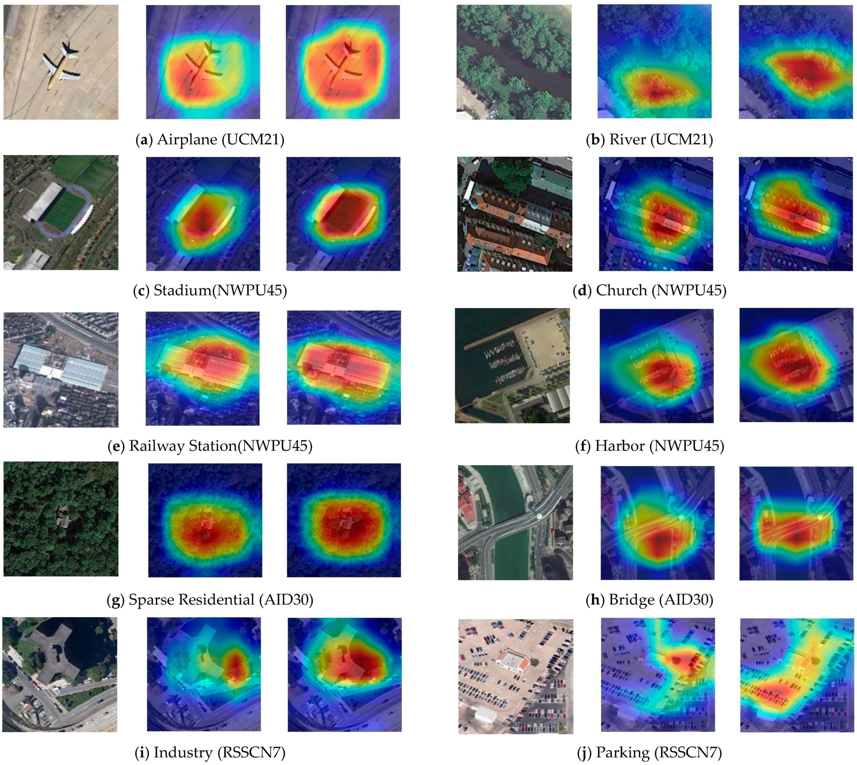
To augment the feature extraction and recognition capabilities in remote sensing image classification tasks, this study proposes a residual network based on the ResNet50 backbone that combines multiple enhanced attention mechanisms, including MSSAM, DCSAM and MSCAM, and is arranged through an HFCE strategy. The network is integrated with a lightweight attention mechanism (MSSAM) designed to extract multiscale features in a shallow network. In the middle network, a dual space and channel attention mechanism (DCSAM) is integrated. In deep layers, the attention mechanism is further strengthened to focus on the features between channels using MSCAM to improve the recognition ability for complex image semantics. Additionally, the optimization of FAS further improves the performance of the attention-enhanced model. The performance of the model is superior to the original network and is stronger than some of the current mainstream models. The experimental results show that the model performs well on multiple datasets. Among them, on the UCM21 dataset, the model’s OA values were as high as 98.76% and 99.77%, achieving nearly saturated performance compared to various recent methods. On the RSSCN7 dataset, the model still demonstrates greatly improved performance. On larger datasets, the model has good recognition ability in NWPU45, especially with a 10% training ratio, which is nearly 1.00% higher than the native network and surpasses most recent networks. This highlights the model’s strengths in handling limited and uneven sample learning. On the AID30 dataset, which is characterized by more complex scenarios and sematic information, the performance improvement of the proposed model is relatively slight but it still maintains a leading position, particularly in its small training ratio. Thus, the improvement of the classification ability of such aerial scenes is the main goal of our work. For visualization, attention heatmaps reveal that, in several cases, the model’s focus becomes more concentrated and its regions of interest more accurate. In the future, our work will also be extended to hyperspectral, low-quality and noisy datasets to expand the application scenarios of the model, thus verifying its universality in remote sensing image classification tasks.