Article

Quantifying the Relationship Between the FPAR and Vegetation Index in Marsh Wetlands Using a 3D Radiative Transfer Model and Satellite Observations

1
Hunan Provincial Key Laboratory of Forestry Remote Sensing Based Big Data & Ecological Security, Central South University of Forestry & Technology, Changsha 410004, China
2
Hunan Key Laboratory of Land Resources Evaluation and Utilization, Hunan Planning Institute of Land and Resources, Changsha 410007, China
3
Hunan Engineering Technology Research Center of Natural Resources Survey and Monitoring, Changsha 410007, China
*
Author to whom correspondence should be addressed.
Remote Sens. 2025, 17(18), 3223; https://doi.org/10.3390/rs17183223
Submission received: 18 July 2025 / Revised: 11 September 2025 / Accepted: 11 September 2025 / Published: 18 September 2025

Abstract

Highlights

What are the main findings?
  • The study quantified the relationship between FPAR and nine vegetation indices (VIs) in marsh wetlands, identifying saturation thresholds: FPAR.inf (saturation onset) ranged from 0.423 to 0.762 (mean = 0.597), while FPAR.sup (saturation point) ranged from 0.786 to 0.921 (mean = 0.857).
  • The NDVI demonstrated the highest predictive accuracy for FPAR before saturation, whereas the EVI was found to be the most effective VI for estimating FPAR after the saturation point occurred.
What is the implication of the main finding?
  • The established saturation thresholds provide critical benchmarks for remote sensing monitoring, indicating that different vegetation indices must be selected for accurate FPAR estimation depending on whether the vegetation is below or above its saturation point.
  • This finding enhances the precision of carbon flux and productivity assessments in wetland ecosystems, which is vital for improving climate change modeling and informing effective ecosystem management strategies.

Abstract

Wetland ecosystems, particularly marsh wetlands, are vital for carbon cycling, yet the accurate estimation of the fraction of absorbed photosynthetically active radiation (FPAR) in these environments is challenging due to their complex structure and limited field data. This study employs the large-scale remote sensing data and image simulation framework (LESS), a 3D radiative transfer model, to simulate FPAR and vegetation indices (VIs) under controlled conditions, including variations in vegetation types, soil types, chlorophyll content, solar and observation angles, and plant density. By simulating 8064 wetland scenes, we overcame the limitations of field measurements and conducted comprehensive quantitative analyses of the relationship between the FPAR and VI (which is essential for remote sensing-based FPAR estimation). Nine VIs (NDVI, GNDVI, SAVI, RVI, EVI, MTCI, DVI, kNDVI, RDVI) effectively characterized FPAR, with the following saturation thresholds quantified: inflection points (FPAR.inf, where saturation begins) ranged from 0.423 to 0.762 (mean = 0.594) and critical saturation points (FPAR.sat, where saturation is complete) from 0.654 to 0.889 (mean = 0.817). The Enhanced Vegetation Index (EVI) and Soil-Adjusted Vegetation Index (SAVI) showed the highest robustness against saturation and environmental variability for FPAR estimation in reed (Phragmites australis) marshes. These findings provide essential support for FPAR estimation in marsh wetlands and contribute to quantitative studies of wetland carbon cycling.

1. Introduction

Wetland ecosystems provide numerous ecological and social benefits, including clean water, flood control, and habitat for wildlife [1,2,3,4]. They are also significant carbon sinks, playing a crucial role in regulating the ecosystem carbon cycle and maintaining carbon balance [5,6]. A key component of this carbon sequestration is net primary productivity (NPP), which represents the net amount of carbon fixed by plants through photosynthesis after accounting for respiration. NPP is therefore an essential indicator for assessing the carbon fixation capacity of wetlands [7]. The fraction of absorbed photosynthetically active radiation (FPAR) reflects the optical properties of the vegetation canopy and is an important parameter for characterizing the vegetation’s photosynthesis level and growth status [8]. FPAR is a critical input in the light use efficiency (LUE) model, which estimates NPP by calculating the product of FPAR, photosynthetically active radiation (PAR), and LUE, representing the efficiency of light conversion into biomass [5]. Coupling remote sensing data with the LUE model has become one of the main approaches employed for the NPP simulation of wetland ecosystems at meso-large scales at present [9]. In the LUE model, both the FPAR and LUE value characterize vegetation’s solar energy absorption and utilization, serving as key covariates that influence NPP estimation accuracy [10]. Therefore, the quantitative description of the FPAR of wetland vegetation represents a crucial topic within the broader field of quantitative models of the wetland carbon cycle [11,12]. Reed (Phragmites australis) marshes are high-carbon-sink ecosystems and herbaceous wetlands that hold a unique position in the carbon cycle and sequestration [13]. However, the reed marsh ecosystem and its carbon sink function are vulnerable to climate change and human activities, and it is a prime area for studying wetland FPAR [14,15].
Remote sensing provides an effective approach for deriving large-scale and temporally continuous FPAR datasets. Primary approaches include empirical and physical methods [14,16,17,18]. Empirical methods commonly involve the following: (1) deriving FPAR from field measurements, (2) calculating vegetation indices (VIs) from canopy spectral measurements or remote sensing imagery, and (3) establishing statistical relationships to develop empirical FPAR–VI regression models [19]. Empirical methods have the advantages of simple principles and efficient solutions, and their use constitutes the main way to obtain the FPAR in the LUE model [14]. However, this widely used approach presents several limitations: (1) estimation accuracy is highly dependent on both remote sensing data quality and ground measurement precision; (2) the FPAR–VI relationships exhibit poor transferability across different ecosystems; and (3) index saturation effects significantly degrade model performance, particularly in dense vegetation canopies [10,15]. Moreover, the water flow in wetlands greatly influences the underlying surface, which complicates the collection of field observation data. As a result, conducting quantitative inversion studies on related surface parameters continues to pose significant challenges [20,21]. Examining the relationship between wetland FPAR and VIs can improve the optimization of empirical models for retrieving the FPAR, leading to more accurate estimations [17,22]. However, current studies on FPAR primarily concentrate on grasslands, forests, and crops [23,24], meaning that comprehensive quantitative analyses of the relationship between FPAR and VIs in marsh wetlands remain limited. To address these limitations and better understand the FPAR–VI relationship in complex wetland environments, advanced modeling approaches are necessary.
Three-dimensional (3D) radiative transfer models incorporating realistic scene geometries (e.g., large-scale remote sensing data and image simulation framework, LESS) can precisely simulate the following: (1) sensor-viewing geometry, (2) solar illumination conditions (including both direct and diffuse components), and (3) 3D canopy radiative transfer effects [25,26]. These models can accurately describe spatial heterogeneity and provide reliable data support for further research, such as quantitative inversion of the FPAR [15]. Furthermore, the use of a radiative transfer model allows for the examination of the relationship between VIs and the FPAR in diverse scenes, which is beneficial for a comprehensive estimation of the uncertainty associated with the FPAR [27]. The contributions of this study can be summarized from the following aspects: (1) we generated a substantial number of scenes based on the 3D radiative transfer model and simulated the VIs and FPAR dataset of a reed marsh; (2) the relationship between FPAR and VIs in different scenes and the influence of factors such as VIs saturation effect and environmental factors on the relationship were quantitatively evaluated; and (3) we developed two indicators (FPAR.inf and FPAR.sat) for the quantitative description of the saturation effect in FPAR estimation. It is our intention to provide the necessary technical and data support for the quantitative study of wetland carbon cycling.

2. Materials

2.1. Study Area

Dongting Lake Wetland is situated in northeastern Hunan Province, China, a region characterized by a subtropical monsoon climate, with an average annual temperature of 15.8–17.4 °C and an annual precipitation of 1200–1500mm [7,28]. Dongting Lake Wetland is a major reed production area in China, contributing more than 30% of the country’s total reed production [29]. Reed marsh vegetation grows in a complex environment, and the mixed vegetation in the understory primarily consists of sedge (Cyperus rotundus L.), which is representative of the area for the study of the relationship between wetland VIs and the FPAR. The experimental area is situated in Liumenzha (112°78′E, 29°46′N), Junshan District, Yueyang City. The present study was performed in this region with an experimental design and a series of detailed field experimental data measurements (Figure 1). The area is a concentrated growth area with good reed and sedge growth and is not affected by artificial reclamation other than natural conditions. The area is characterized by reed and sedge mixed-growth (RSS), in addition to reed monoculture (RS, which is regarded as RS if the density of sedge in the sample plot is less than 1/5 of that of reeds), rendering it an optimal site for field data collection and simulation studies.

2.2. Sample Setting

A total of 10 RS plots and 10 RSS plots were selected in the experimental area of the reed marsh in Dongting Lake. Scene characteristics were measured by establishing five 1 m × 1 m subplots along the diagonal of each main sample plot. The mean value across these subplots represents the plot-level scene characteristic measurement. Individual plant characteristics were assessed by randomly selecting three healthy plants within each main plot. The average of these measurements represents the plot-level value for plant characteristics. The subsequent aerial photography process, performed using a UAV, and the field surveys were performed in the experimental area and sample plots.

2.3. Field Survey

Field surveys were conducted in April, May, and June 2023–2024. For each specimen, we collected individual plant characteristics comprising the following: (1) structural traits (plant height, stem width, leaf spacing), (2) leaf morphological characteristics (number, length, width, inclination angle, and height), and (3) leaf physiological parameters (chlorophyll, carotenoids, water thickness, and dry matter). We collected scene characteristics comprising the following: (1) canopy spectra and FPAR, (2) population metrics (density and competitive proportions), and (3) environmental factors (soil moisture and spectra, solar angles, and observation angles). The objective of acquiring the growth data was to construct 3D models of individual plants and scenes.
First, we measured the structural and leaf characteristics of the sampled plants with the aid of a ruler, tape measure, and ladder. To determine the leaf morphological characteristics, we measured all of the healthy leaves of the sample plants. Specifically, the leaf inclination angle was measured in segments using a LAMDA (leaf angle measurement device alpha version). Thereafter, two green leaves were collected from both the upper (>1 m height) and lower (≤1 m height) canopy layers per sampled plant for physiological parameter measurement. The fresh weight of the leaves was first measured. After drying, the dry weight of the leaves was measured as the dry matter. The leaf area was measured using a YMJ-PC leaf area meter. Lastly, the leaf equivalent water thickness was calculated using Equation (1):
Leaf   equivalent   water   thickness   =   fresh   weight     dry   weight leaf   area
To account for heterogeneous chlorophyll distribution, each leaf was divided into three equal sections, and 0.1 g of each section was taken for the determination of chlorophyll content. The mean chlorophyll content across all 12 measured sections (4 leaves × 3 sections) was calculated to represent the sampled plant chlorophyll content. The chlorophyll content was measured using a spectrophotometer, and values were obtained by determining the optical density of the 80% acetone extract at different wavelengths. The contents of chlorophyll and carotenoids were calculated using Equations (2)–(5) [30]:
Chlorophyll   a = 13.95 × A 665 6.88 × A 649
Chlorophyll   b = 24.96 × A 649 7.32 × A 665
Cab = Chlorophyll   a + Chlorophyll   b
carotenoids = 1000 × A 470 2.05 × Chlorophyll   a 114.8 × Chlorophyll   b 245
where A665, A470, and A649 represent the absorbance of the chlorophyll pigment extract at wavelengths of 665 nm, 470 nm, and 649 nm, respectively. The total chlorophyll concentration (Cab) was calculated using Equation (4).
With the aid of a ladder, the canopy spectra of a 1 × 1 m subplot were collected using a high-performance spectrometer, HR-1024i (Spectra Vista Corporation, Poughkeepsie, NY, USA), with 1024 bands covering the region of wavelengths from 350 nm to 2500 nm. The soil moisture content of each subplot was determined by using a soil moisture tester (in particular, for flooded soil, we only measure the submergence height). Thereafter, soil spectra measurements were also performed under three soil moisture conditions: flooded soil (F, the soil was submerged by water), moderate soil (M, 15–30% volumetric water content), and wet soil (W, >30% volumetric water content). For each subplot, three replicate measurements were averaged to determine mean reflectance values. While the solar zenith angle (SZA), solar azimuth angle (SAA), observation zenith angle (VZA), and observation azimuth angle (VAA) were measured in unison, the optical properties of the canopy and soil were precisely defined, thereby providing verification data for the spectral characteristics of the canopy in the complex environment of reed marshes.
We employed a SunScan canopy analysis system (measurement accuracy ± 10%) to quantify PAR components: (1) canopy-absorbed PAR, (2) canopy-reflected PAR, (3) transmitted PAR reaching the soil surface, and (4) soil-reflected PAR. Multi-directional PAR measurements (diagonal, vertical, and horizontal) enabled calculation of the FPAR, supporting validation of VI-FPAR relationships.

2.4. Remote Sensing Data and Other Auxiliary Data

In this study, we collected aerial imagery (used for mapping the overview of the study area) from the experimental marsh using an unmanned aerial vehicle (DJI Mavic 3E, DJI, Shenzhen, China) that includes an embedded RGB camera. The resolution of the images was 26,574 × 32,005 pixels with a sampling distance of 3 cm per pixel. The Sentinel-2 dataset (ID: COPERNICUS/S2_SR_HARMONIZED) was obtained from the Google Earth Engine platform, and the reflectance data captured in April, May, and June 2023–2024 were selected for the calculation of VIs. In addition, the auxiliary data included a land cover dataset [31] and administrative boundary data.

3. Methods

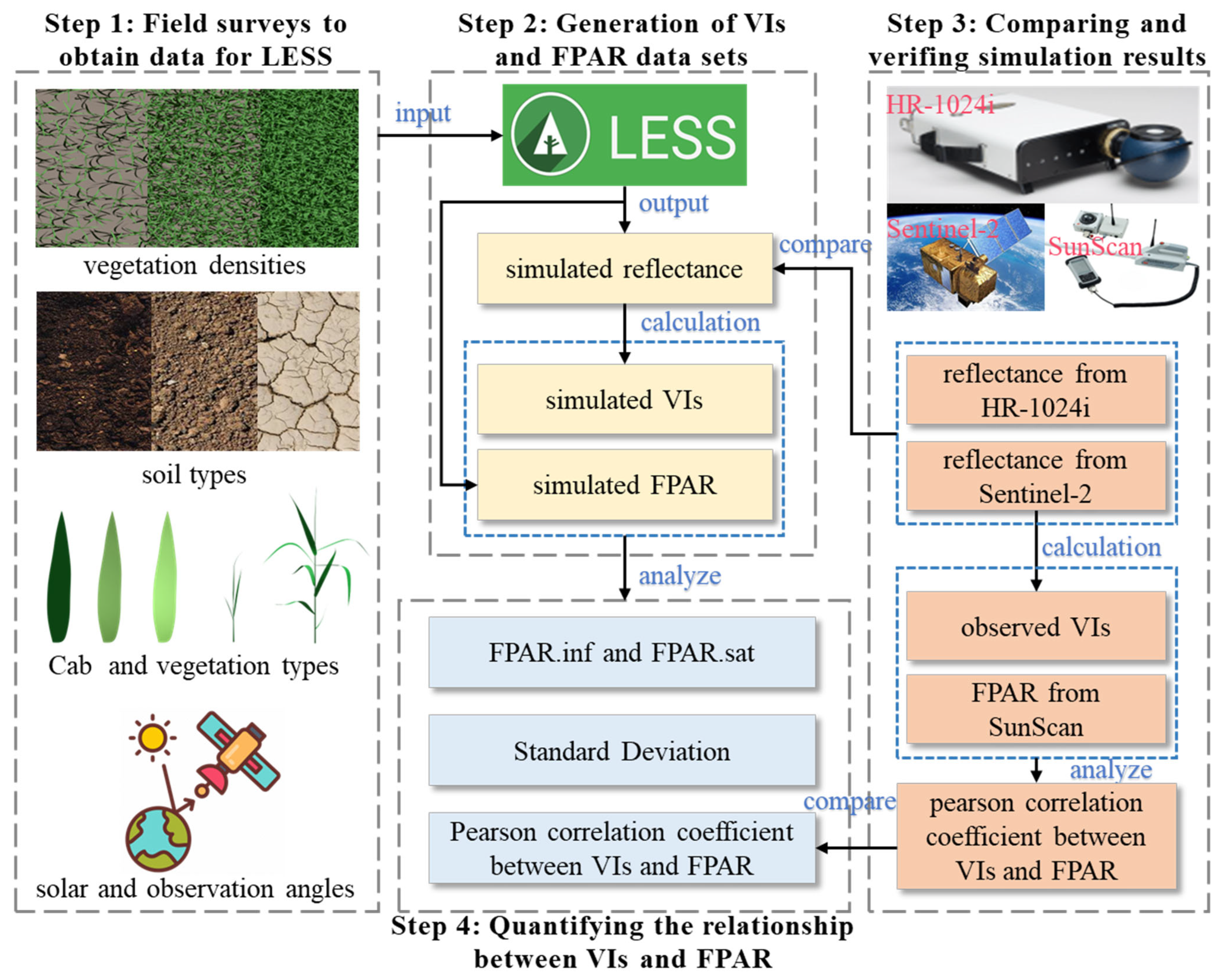
In this study, we implemented a four-step quantitative framework (Figure 2) to assess VI-FPAR relationships using the 3D radiative transfer model LESS (LESS-2.1.5): Step (1) Scene construction: Field-derived structural parameters were parameterized in LESS to generate realistic reed marsh scenes. Step (2) Dataset generation: Model outputs provided both FPAR and hyperspectral reflectance data for VI calculation. Step (3) Validation: Simulation results were verified against ground- and satellite-based reflectance measurements. Step (4) Relationship quantification: We evaluated VI-FPAR relationships through the following means: (i) Pearson’s r, (ii) variability analysis (SD), and (iii) saturation metrics (FPAR.inf and FPAR.sat).

3.1. Basic Principles of LESS

LESS employs a triangular mesh-based architecture to reconstruct 3D vegetation scenes with high fidelity. Its bidirectional ray-tracing algorithms precisely capture the spectral properties and structural attributes of canopy components [32]. The model enables high-precision simulations of remote sensing signals in meso- to large-scale scenes, eliminating errors from scene simplification. In addition, it accurately simulates vegetation canopy reflectance and the FPAR absorption process [33,34,35,36], facilitating quantitative inversion of canopy FPAR and saturation effect analysis [37]. Since solar radiation absorbed by woody components does not contribute to photosynthesis, LESS can further refine the FPAR simulation by focusing on leaves, improving accuracy. Simulating FPAR–VI correlations across diverse scenes reduces fieldwork costs and measurement errors, which is critical for advancing FPAR estimation uncertainty research.

3.2. Reed Marsh Scene Construction

3.2.1. Simulation of Leaf Spectrum

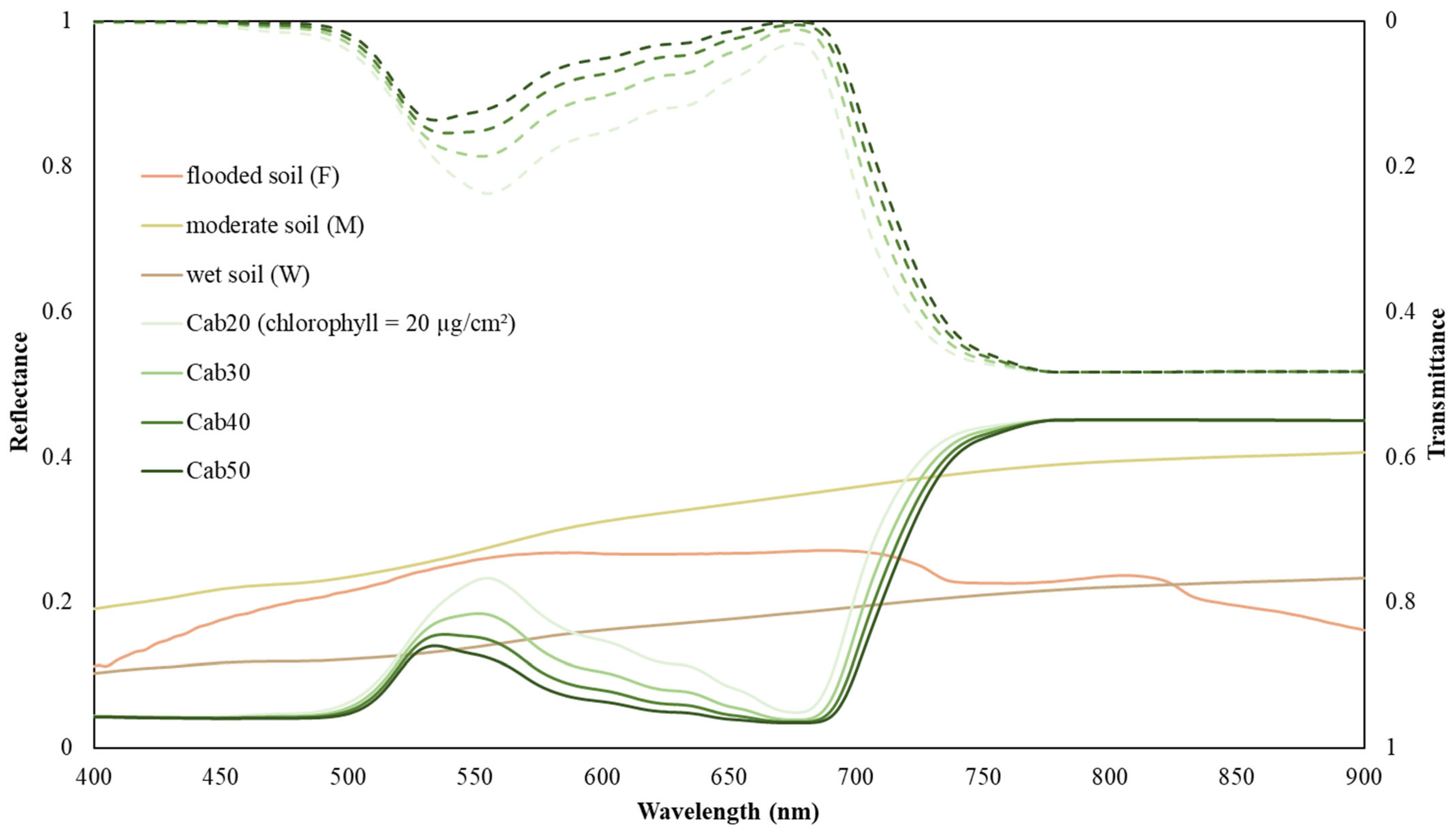
PROSPECT-5 is a widely used leaf radiative transfer model [38], simulating leaf spectra across the range of 400–2500 nm. Its input parameters include the following: (1) the structural parameter N (leaf cell density) and (2) biochemical parameters (Cab, carotenoids, water thickness, and dry matter). Seasonal changes induce variations in the pigments of reed leaves, which in turn lead to changes in the leaf spectra. Given that Cab has the greatest influence on the leaf spectrum [39,40], we only changed the Cab level to simulate the leaf spectra of reeds in different seasons. Moreover, since direct measurement was not possible, the structural parameters N of both reed and sedge were set to the empirical value of 1.5 [41]. The fixed PROSPECT-5 parameters of the reed were as follows: N = 1.5, carotenoids = 8 µg/cm2, water thickness = 0.012 cm, and dry matter = 0.007 g/cm2. Four Cab levels (20, 30, 40, and 50 µg/cm2, denoted as Cab20–Cab50) were investigated. The fixed PROSPECT-5 parameters of sedge were as follows: N = 1.5, carotenoids = 0.7 µg/cm2, water thickness = 0.03 cm, Cab = 30 µg/cm2 (to simplify the scene and reduce unnecessary calculations, the Cab in sedge was set to a constant based on the measurement), and dry matter = 0.008 g/cm2. Figure 3 shows the spectra of reed leaves and soil.

3.2.2. Modeling of a Single Plant

Using field measurements from Dongting Lake Wetland reed samples, we developed high-precision 3D single-plant reed models through Blender (Blender-3.6.4) and image-based photogrammetry [42] to maximize morphological accuracy. We applied the same methodology to model sedge plants, which coexist in the reed marsh understory. These individual plant models provided essential geometric data for subsequent wetland scene reconstruction.

3.2.3. Modeling of the Reed Marsh Scene

The scene model comprised multiple randomly distributed 3D plant models, together with solar angles, observation angles, and soil background. To reflect natural growth patterns, plant components maintained specific topological relationships in 3D space [43], including enforcing minimum spacing between plants to prevent complete overlap, intersection, or spatial sharing.
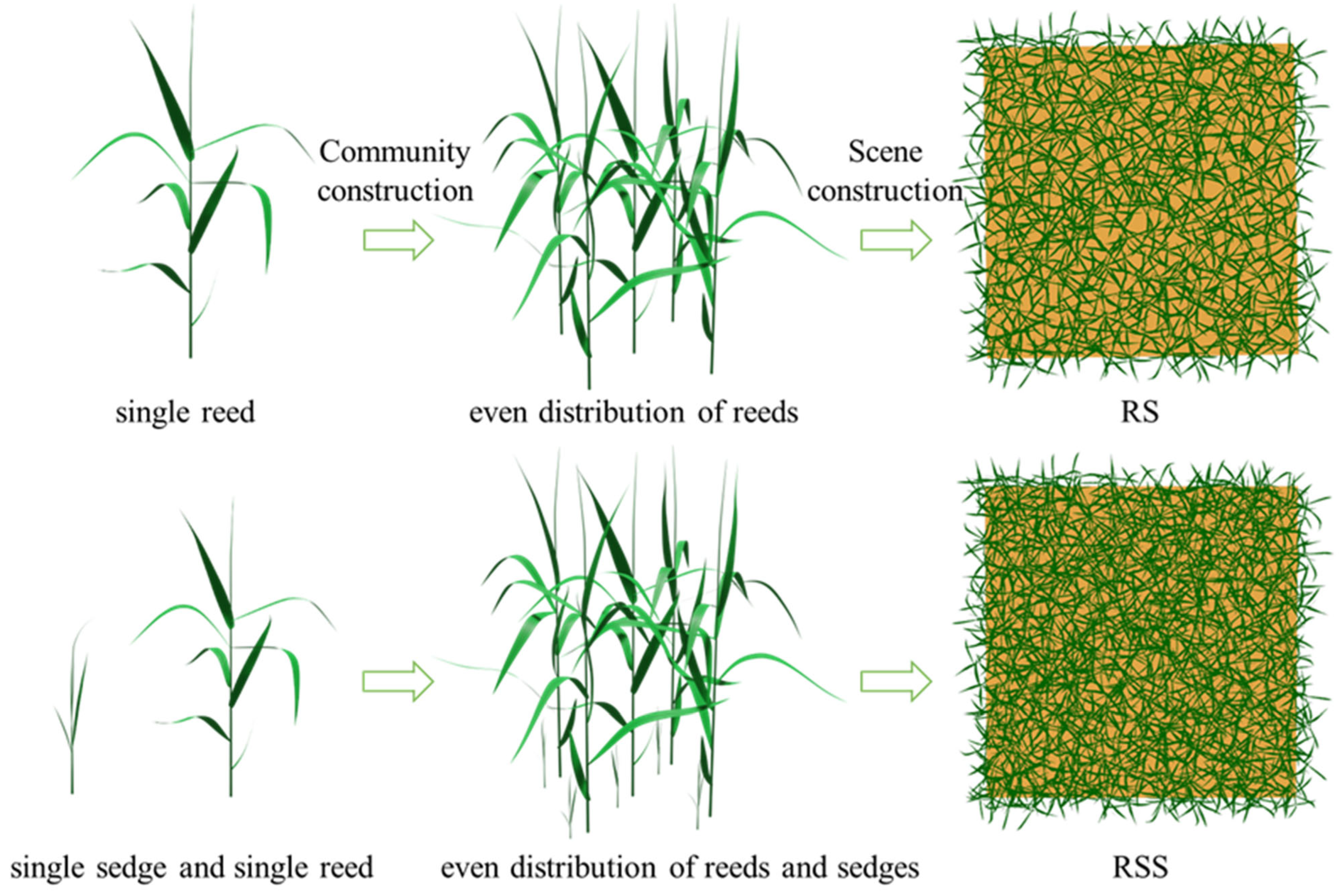
To obtain FPAR and VIs, we generated 8064 simulated scenes. These scenes incorporated 28 plant densities, 2 vegetation types (RS and RSS), 4 Cab levels, 3 soil types, 3 solar angles, and 4 observation angles (based on field surveys). In Table 1, the parameter configurations for the LESS model are summarized, with Figure 4 illustrating the modeling workflow of the reed monoculture scene and the mixed-growth scene. The setting of parameters was guided by the actual growth patterns and distribution of reeds in the study area.

3.3. Verification of the Simulation Accuracy of Reed Marsh Canopy Reflectance

Multispectral (B2–B6 and B8) and hyperspectral observations (400.9–900.5 nm, 375 bands) from the Sentinel-2 and the HR-1024i spectrometer were used to assess the accuracy of the LESS model for reed marsh canopy spectra. The LESS simulations covered 400–900 nm at a 1 nm spectral resolution. To enable comparison, the simulated reflectance data were resampled to match the 375 hyperspectral bands and the 6 Sentinel-2 multispectral bands. The root mean square error (RMSE) and the index of agreement (d) [44] were employed to evaluate the simulation accuracy of reed marsh canopy reflectance. These metrics were calculated as follows:
R M S E = 1 n i = 1 n R i , o b s R i , s i m 2
d = 1 i = 1 n R i , o b s R i , s i m 2 i = 1 n R i , o b s R i , o b s ¯ + R i , s i m R i , o b s ¯ 2
where n is the number of hyperspectral and multispectral bands, R i , o b s and R i , s i m are the observed and simulated values of reflectance, respectively, and R i , o b s ¯ is the mean value of the observed reflectance values.

3.4. VIs Calculation

In order to meet practical application requirements and reduce the incidence of errors, the hyperspectral reflectance simulated by LESS was converted into reflectance of six satellite spectral bands, namely, Blue (B), Green (G), Red (R), Red Edge 1 (RE1), Red Edge 2 (RE2), and NIR, in combination with the spectral response function of Sentinel-2 [45]. The following nine VIs exhibit a high degree of correlation with the FPAR: the Normalized Difference Vegetation Index (NDVI), Green Normalized Difference Vegetation Index (GNDVI), Soil-Adjusted Vegetation Index (SAVI), Ratio Vegetation Index (RVI), Enhanced Vegetation Index (EVI), Meris Terrestrial Chlorophyll Index (MTCI), Difference Vegetation Index (DVI), kernel Normalized Difference Vegetation Index (kNDVI), and Renormalized Difference Vegetation Index (RDVI) [46,47]. The information presented in Table 2 illustrates the calculation formulas for each VI. Following the simulation of canopy reflectance and calculation of the VIs, the nine VIs were normalized in order to obtain the same dynamic range, thus facilitating comparison and subsequent result analysis, as follows:
V I N = V I V I m i n V I m a x V I m i n
where V I m a x and V I m i n are the maximum and minimum values of VIs in a set of 28 density reed marsh scenes, and V I N is the normalized value of VIs.

3.5. Quantifying the Relationship Between VIs and the FPAR

The LESS model simulated 8064 wetland scenes, incorporating 2 vegetation types (RS and RSS), 3 soil types, 4 Cab levels, 3 solar angles, 4 observation angles, and 28 plant densities. Since observation angles do not impact the FPAR in LESS, 2016 unique FPAR values were generated, with each corresponding to VI values across the four observation angles. We evaluated five regression models (linear, polynomial, exponential, logarithmic, and power) for estimating the FPAR from VIs and selected the optimal model based on model performance. Model performance was assessed through the comparative analysis of determination coefficients (R2s) and root mean square errors (RMSEs):
R 2 = 1 i = 1 n ( FPAR i FPAR ^ i ) 2 i = 1 n ( FPAR i FPAR ¯ ) 2
RMSE = 1 n i = 1 n ( FPAR i FPAR ^ i ) 2
where FPAR i is the i-th observed FPAR value, FPAR ^ i is the i-th model-predicted FPAR value, FPAR ¯ is the mean of observed FPAR values, and n is the sample size.
Sensitivity analyses were performed to quantify progressive changes in VIs with increasing FPAR and assess the impact of VI saturation on FPAR estimation accuracy. Using Equation (11), we evaluated Slope, with decreasing Slope indicating diminished VI responsiveness to FPAR variations, revealing saturation effects. Using Equation (12), we evaluated VI dispersion using standard deviation (SD). A higher SD indicated that the VI was more sensitive to the scene conditions, as follows:
S l o p e = y i y i 1 F P A R i F P A R i 1
S D = 1 n 1 i = 1 n y i y ¯ 2
where y i and FPAR i are the i-th simulated V I N and FPAR value, respectively, y ¯ is the mean of V I N values, and n is the sample size.
VI-FPAR correlations degrade beyond a critical vegetation density threshold due to saturation effects, limiting measurement precision. Building on established saturation evaluation frameworks [37], we propose two novel thresholds: the saturation inflection point (FPAR.inf) and saturation critical point (FPAR.sat). Based on the remarkable segmented trend between the VI–FPAR response relationship, the VI-FPAR relationship is modeled as a piecewise linear function, as follows:
VI = k 1 × FPAR + b 1 FPAR x k k 2 × FPAR + b 2 FPAR > x k
where x k (equivalent to FPAR.inf) marks the transition between linear ( k 1 ) and nonlinear ( k 2 ) regimes, determined by minimizing the fitting error (MAE + continuity penalty). FPAR.sat is defined as the FPAR value where the VI Slope (Equation (11)) falls below 0.1 [37]. The results presented in Figure 5 detail the computational workflow, including iterative optimization for x k identification and Slope thresholding.

4. Results

4.1. Canopy Spectrum and the FPAR Simulation Accuracy of LESS

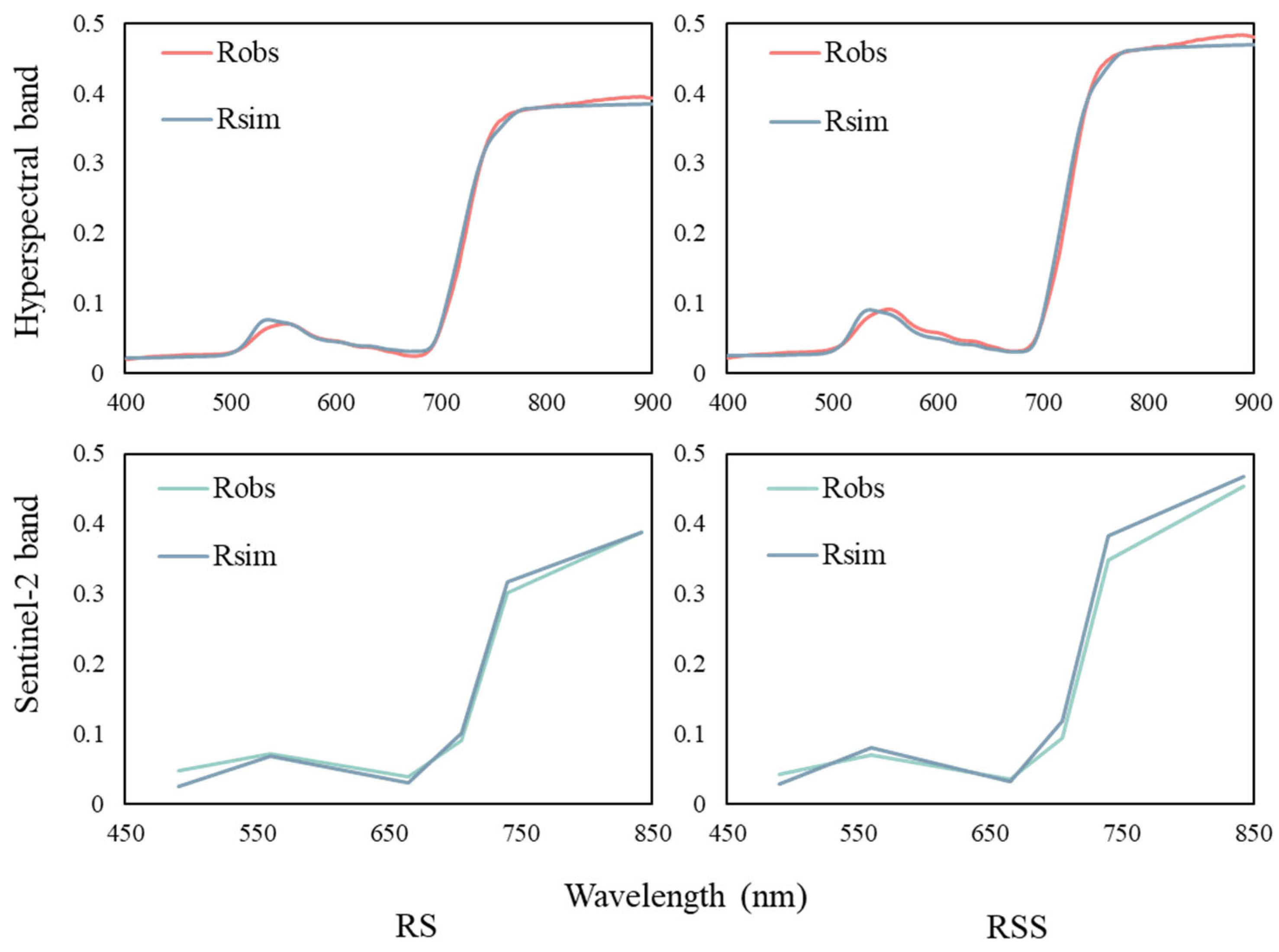
The LESS-simulated reflectance spectra for both RS and RSS (under typical conditions during the research period: M soil type, Cab30, solar angles 10:130, observation angles 30:270, and 40 plants/m2) showed strong agreement with field measurements from Sentinel-2 and HR-1024i (Figure 6). Notably, RS demonstrated marginally better spectral simulation accuracy than RSS. Comparative analysis revealed maximum reflectance discrepancies (Robs–Rsim) of 0.011 for RS and 0.030 for RSS when validated against HR-1024i hyperspectral data. For Sentinel-2 multispectral data, simulated reflectance exhibited wavelength-dependent biases: at B6’s central wavelength, Rsim overestimated observations by 0.016 (RS) and 0.033 (RSS); in comparison, at B2’s wavelength, it underestimated observations by 0.023 (RS) and 0.015 (RSS). The high consistency between the observed and simulated reflectance was further confirmed through agreement indices (d ≥ 0.999) and RMSE values. Hyperspectral validation yielded lower errors (RMSE = 0.006 for RS and 0.009 for RSS) compared to multispectral validation (approximately double these values; Figure 7). These results collectively demonstrate LESS’s capability to accurately simulate reed marsh spectral characteristics.
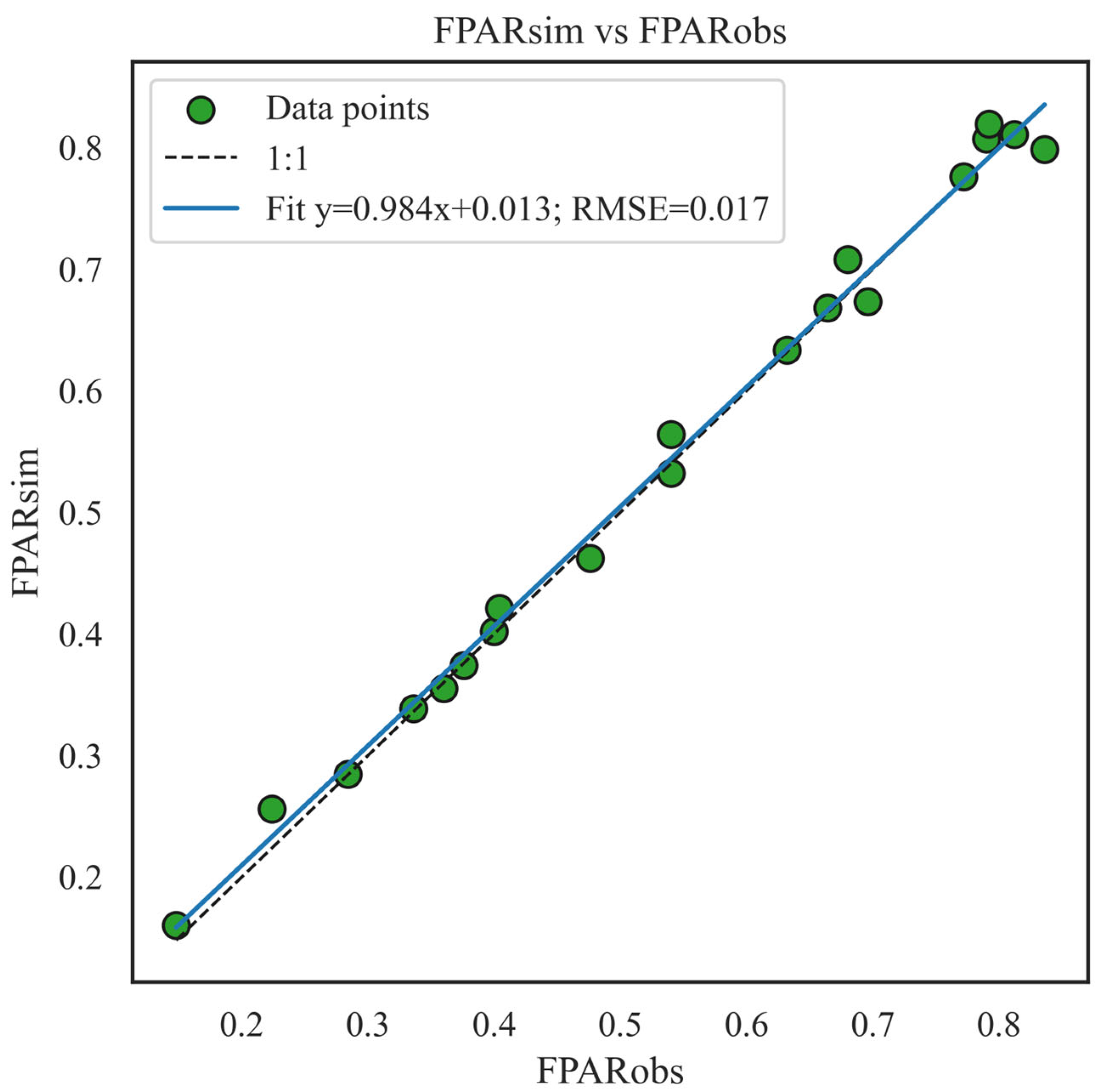
Across the 20 plots, the LESS model reproduced field FPAR from the SunScan system with very small errors (Figure 8). The RMSE was about 0.017 (≈3% of the mean observed FPAR), indicating tight agreement. The maximum absolute deviation was roughly 0.038 and occurred at a higher FPAR site. The fitted linear relationship (FPARsim = 0.98 × FPARobs + 0.013) showed a near-unity slope with a small positive intercept, implying a slight compression at the upper end (mild underestimation of higher values) but no practically significant systematic distortion. Overall, the model provided stable and reliable plot-scale FPAR estimates suitable for subsequent analyses and applications.

4.2. Correlation Between VIs and FPAR

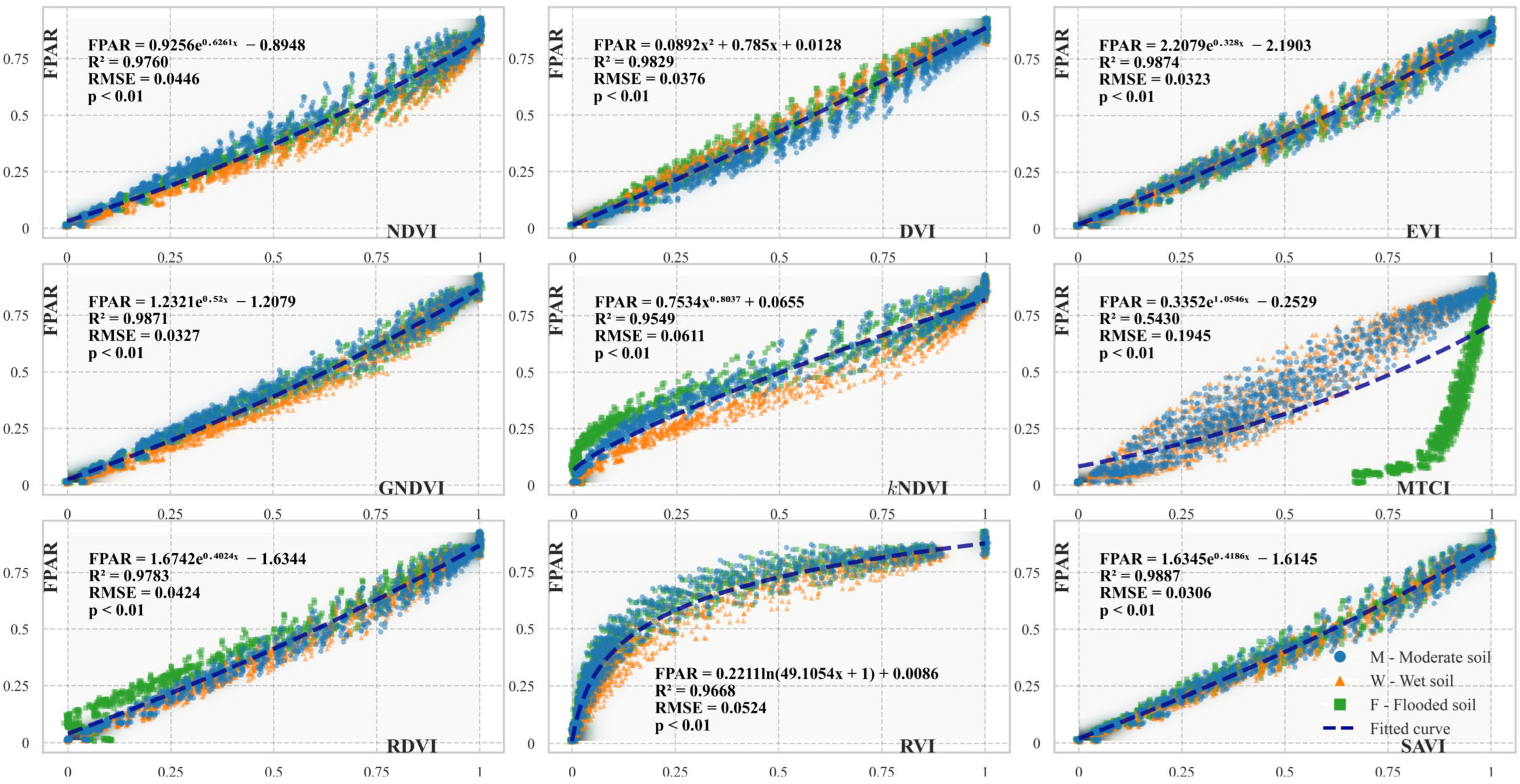
In this study, we developed VI-FPAR fitting models and calculated corresponding R2 and RMSE values. Figure 9 and Figure 10 illustrate the relationships between VIs and the FPAR for RS and RSS, respectively. Compared to RS, RSS generally showed reduced VI-FPAR correlation strength (lower R2) and higher RMSE values. However, one exception was noted: MTCI exhibited better FPAR estimation performance in RSS. Most VIs (except MTCI) demonstrated strong predictive capability for the FPAR (R2 > 0.919 in all cases), with RMSE values consistently below 0.082. The MTCI–FPAR relationship under flooded soil conditions deviated significantly from other moisture regimes, yielding reduced R2 (0.751) and elevated RMSE (0.195). Analysis of MTCI’s formulation (RE2 − RE1)/(RE1 − R) revealed that water may greatly affect the red-edge band reflectance of the reed scene. Consequently, red-edge-based VIs demonstrated limited operational reliability in seasonally flooded wetlands with high hydrological variability.
Most VIs (excluding RVI) exhibited stronger saturation effects in RSS compared to RS, particularly showing stagnated VI responses despite increasing FPAR values in high-VI ranges. This observation aligns with previous findings in grassland, forest, and agricultural ecosystems [50]. In RSS, soil type significantly influenced VI-FPAR relationships. Notably, F produced distinctly different VI-FPAR correlations compared to other soil types.

4.3. Sensitivity of VIs to Scene Conditions

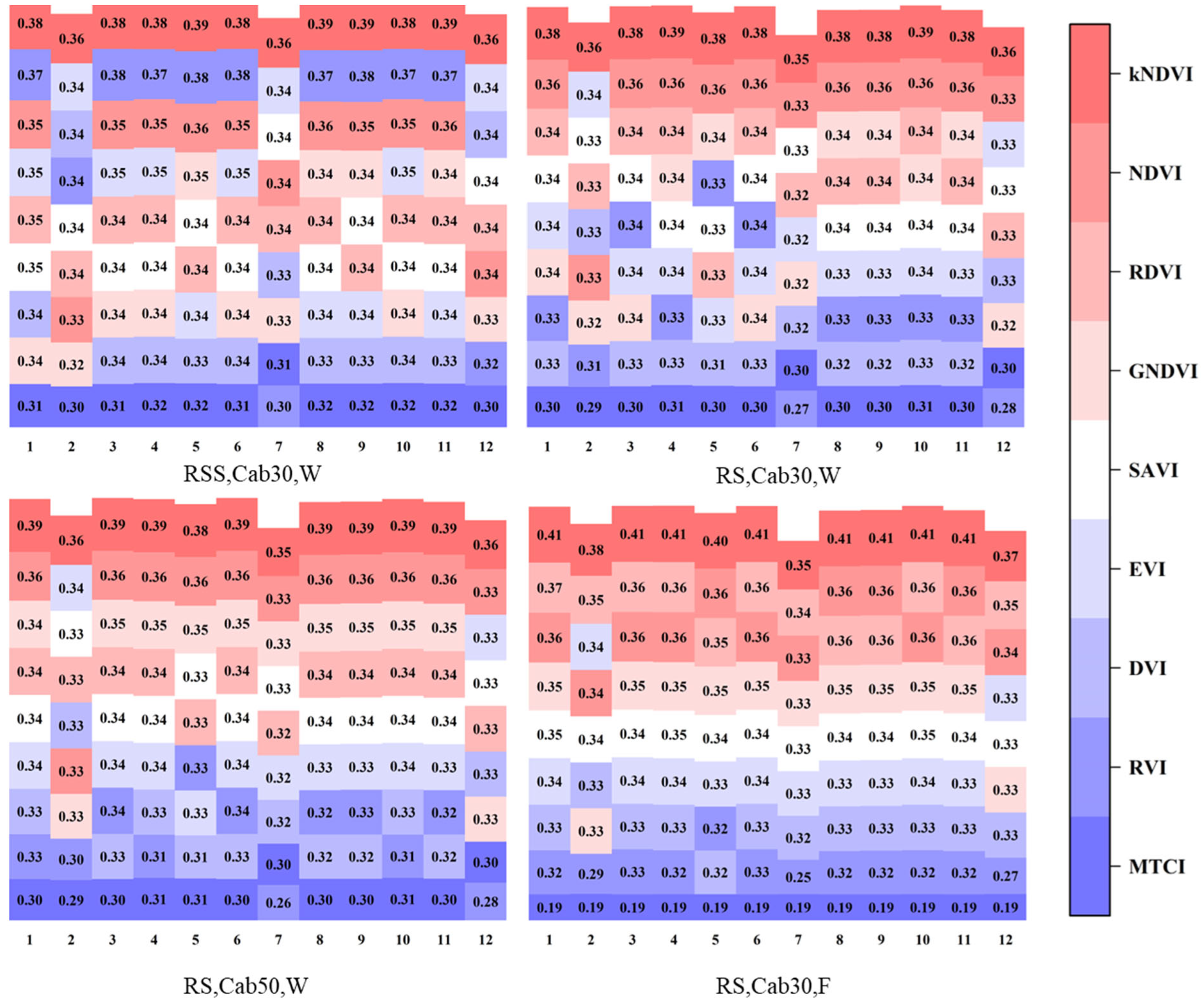
VI performance variations were observed across 12 angular configurations, including three solar angles (SZA:SAA—45°:90°, 10°:130°, and 30°:270°) and four observation geometries (VZA:VAA—0°:0°, 45°:90°, 10°:130°, and 30°:270°). The SD of VIs in the marsh was analyzed as a proxy for sensitivity, where higher SD values indicate greater sensitivity to angular configurations. Under typical experimental conditions (Figure 11), VI SD values ranged from 0.189 to 0.412. The indices were ranked in descending order of mean SD values: kNDVI (0.383), NDVI (0.351), RDVI (0.343), GNDVI (0.340), SAVI (0.339), EVI (0.337), DVI (0.329), RVI (0.326), and MTCI (0.277). kNDVI demonstrated the strongest sensitivity with a mean SD of 0.383, followed by NDVI with a mean SD of 0.351. MTCI showed the lowest sensitivity with a mean SD of 0.277. Despite this, MTCI was still not recommended for the inversion of wetland FPARs due to its poor performance in FPAR fitting (R2 < 0.751).
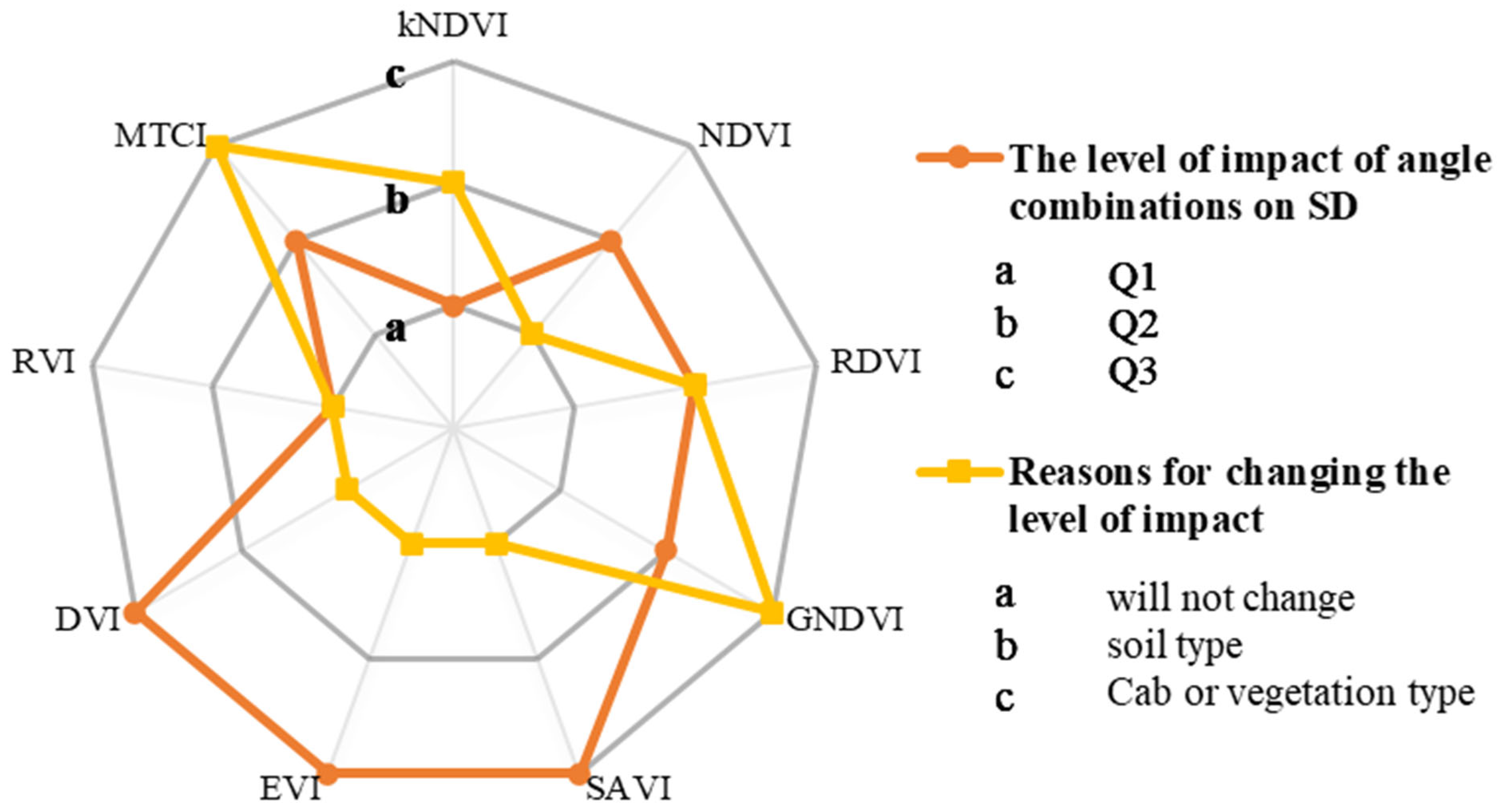
The influence of angular configurations on VI sensitivity was quantified through SD ranges (SDmax–SDmin) across 12 angle combinations. MTCI exhibited the smallest SD range (0.003) under RS, Cab30, and F conditions. Angle impacts were categorized into three tiers: Q1 (strong: SD range > 0.040), Q2 (medium: 0.020–0.040), and Q3 (weak: 0–0.020). Classification followed hierarchical rules: Q1 if any scene showed Q1-level influence; Q2 if only medium influence occurred without Q1 effects; and Q3 if neither Q1 nor Q2 impacts were observed. As shown in Figure 12, four VIs fell into Q2, two VIs (kNDVI and RVI) fell into Q1, and three (DVI, EVI, and SAVI) fell into Q3. VI SD variations were also Cab-, vegetation-, and soil-dependent. kNDVI achieved the highest mean SD (0.383) and showed Q1 angular sensitivity and environmental dependency. Conversely, DVI, EVI, and SAVI maintained angular stability (Q3) and scene adaptability.

4.4. FPAR-Estimated Saturation Inflection Point (FPAR.inf) and Critical Point (FPAR.sat) Analysis

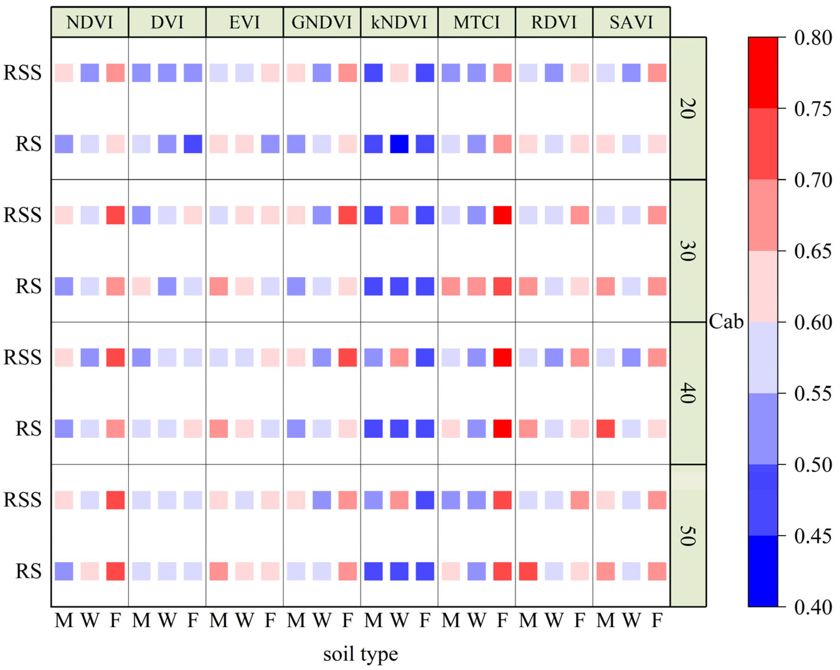
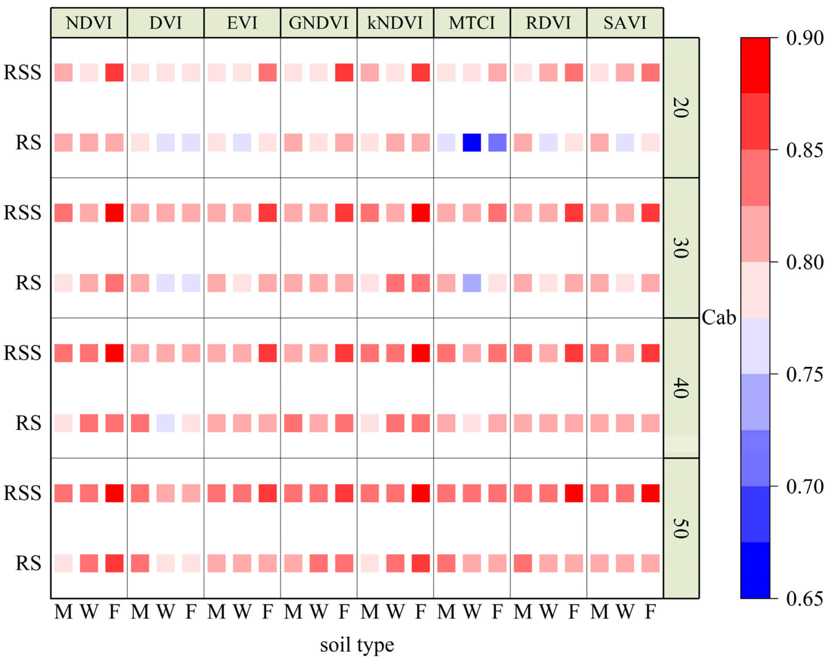
The FPAR.inf and FPAR.sat values were quantified across soil–vegetation–Cab combinations (Figure 13 and Figure 14). RVI was excluded from saturation effects analysis due to its absence of saturation behavior. The FPAR.inf values ranged from 0.423 to 0.762 (mean = 0.594), peaking for MTCI (0.762, RSS/Cab40/F) and reaching minima for kNDVI (0.423, RSS/Cab50/F). The FPAR.sat ranged from 0.654 to 0.889 (mean = 0.817), with MTCI showing minimum (0.654, RS/Cab20/W) and kNDVI showing maximum (0.889, RSS/Cab50/F).
Both FPAR.inf and FPAR.sat generally varied with Cab when averaged across vegetation and soil types, with kNDVI showing the most notable FPAR.sat increase (Δ = 0.076). FPAR.inf for MTCI decreased by 0.042 with Cab. kNDVI, NDVI, and DVI maintained high stability (Δ ≤ 0.015), outperforming other VIs in high Cab-variability regions, though kNDVI’s mean FPAR.inf (0.508) indicated early saturation. Soil moisture significantly altered FPAR.inf: RDVI and SAVI show variations up to 0.138, GNDVI and NDVI varied by 0.116–0.133, and MTCI (RS) exhibited minimal sensitivity at Cab = 20–30 (Δ ≤ 0.019). FPAR.sat remained stable across soils (average range ≤ 0.032 for all VIs).
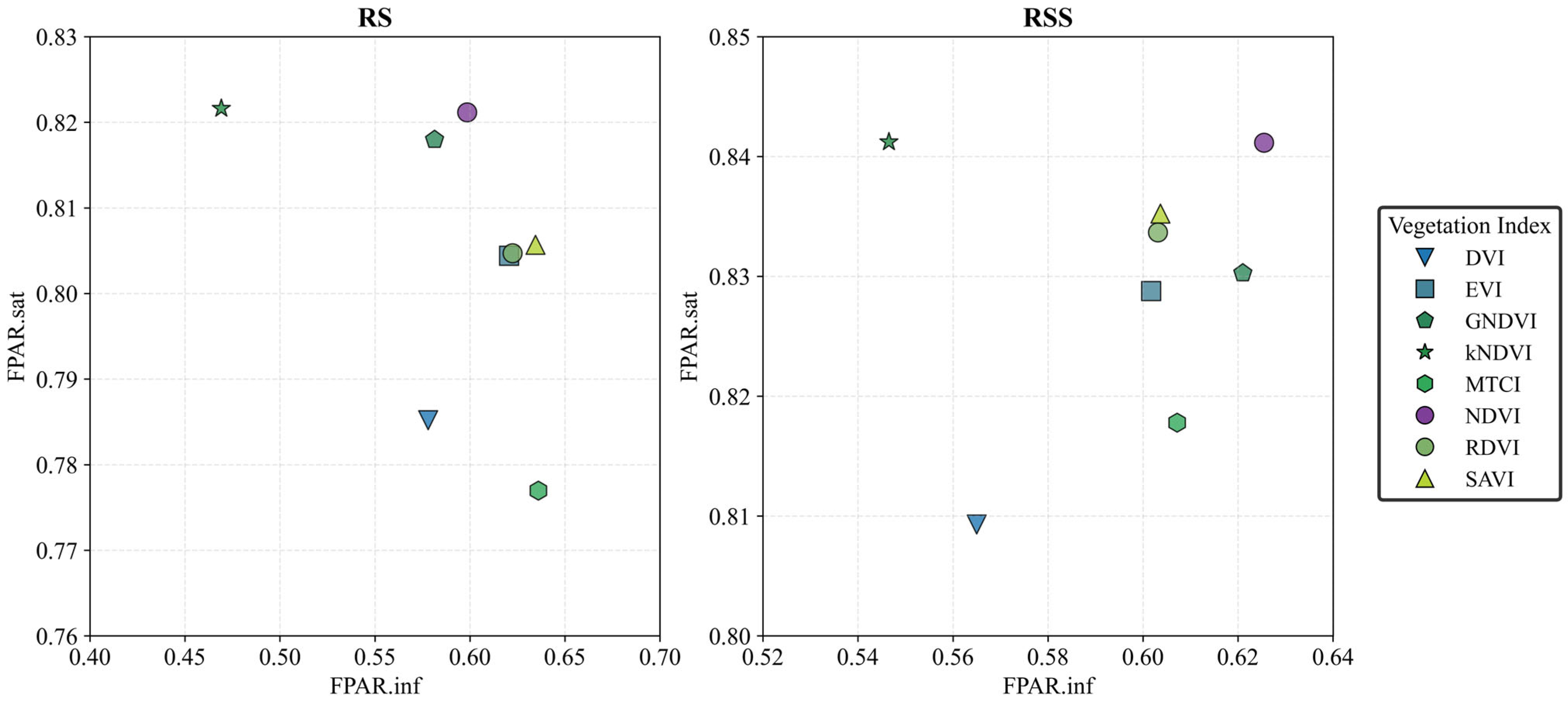
The mean FPAR.inf and FPAR.sat of VIs were quantified for RS and RSS by averaging across Cab levels and soil types (Figure 15). Significant differences in FPAR.inf were observed between vegetation types. While kNDVI, NDVI, and GNDVI showed higher values in RSS (Δ = 0.027 to 0.077), DVI, EVI, RDVI, SAVI, and MTCI exhibited reduced FPAR.inf in RSS (Δ = 0.013 to 0.031). EVI, RDVI, MTCI, and SAVI maintained the highest mean FPAR.inf values (0.601–0.635) across both vegetation types. The introduction of sedge led to the delay of FPAR.inf in the estimation of FPAR by kNDVI, NDVI, and GNDVI, yet the advancement of the other VIs. The influence of vegetation types on FPAR.sat was very uniform. The introduction of sedge led to an increase in FPAR.sat for all indices. The effect on MTCI was the most obvious, increasing by 0.041, followed by SAVI (0.030), and finally the relatively stable GNDVI (0.012).

4.5. Model Transferability and Cross-Ecosystem Validation

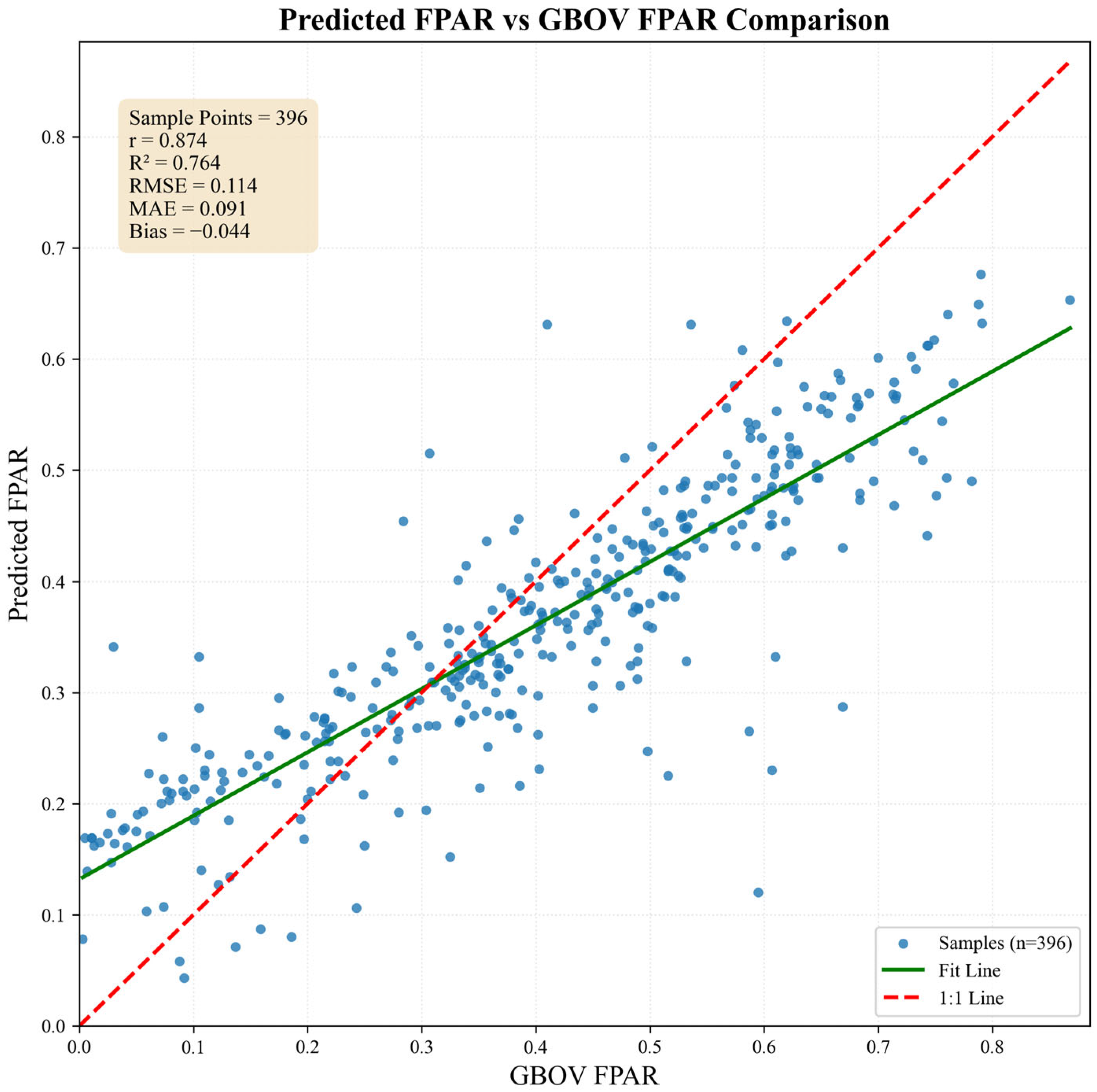
To evaluate the transferability of the wetland FPAR prediction model (based on SAVI) to different ecosystem types, the trained model was applied to grassland vegetation at the WOOD site from the Ground-Based Observations for Validation (GBOV) database [51]. The validation was conducted using GBOV FPAR measurements collected on 27 June 2020, which served as reference data due to the limited availability of wetland FPAR observations. Sentinel-2 surface reflectance imagery (COPERNICUS/S2_SR_HARMONIZED) with less than 30% cloud coverage was acquired for the same date and processed through Google Earth Engine. Predicted FPAR data were resampled to a consistent spatial resolution with the observed data, and 500 random sampling points were generated within the study area, with data quality filters applied to retain only valid FPAR values within the range of 0–1, resulting in 396 valid sample points for accuracy assessment. The statistical evaluation revealed a moderate correlation between predicted and observed FPAR values (r = 0.874, p < 0.001, R2 = 0.764), with a root mean square error (RMSE) of 0.114 and a mean absolute error (MAE) of 0.091 (Figure 16). The model exhibited a systematic underestimation bias of −0.044, indicated by the regression slope of 0.571 and intercept of 0.132, suggesting that the wetland-trained model tends to underpredict FPAR values when applied to grassland ecosystems. Despite this bias, the strong correlation coefficient demonstrates the model’s ability to capture the overall spatial patterns of FPAR variation in grassland environments, though ecosystem-specific calibration would be necessary for optimal accuracy.

5. Discussion

5.1. Factors Affecting the Relationship Between VIs and FPAR

The correlation between the selected VIs and FPAR was highly significant, indicating that the simulated VIs are effective at characterizing the FPAR and have potential for use in reflecting vegetation health status and biomass. In the constructed reed marsh scenes, when the vegetation exceeded a certain density (62 plants/m2 of reed), VI was fully saturated and no longer exhibited a correlation with the density or FPAR. This factor resulted in a Slope value of 0 and an FPAR in the full saturated region. The simulation of ultra-high-density scenes resulted in an increase in the overall simulation time without any discernible improvement in the accuracy of the entire simulation process. Accordingly, the fully saturated region was not a primary focus in this study, which may result in a high R2 value. The factors responsible for VI saturation can be attributed to two aspects: the mathematical formula and reflectance saturation [37]. For example, the NDVI is prone to saturation in areas with high vegetation coverage. In addition to the fact that the red band is prone to saturation [52], the NDVI formula itself is hindered by the fact that it is easily saturated. As vegetation density increases, RED reflectance decreases toward zero. This makes the NDVI denominator (NIR + RED) ≈ NIR, driving NDVI toward one. Further density increases cause negligible RED change, making NDVI insensitive to additional biomass growth. The RVI (ratio of the near infrared band to the red band) increases rapidly when the density is high and is not impacted by saturation effects. This change can be explained by the fact that when the red band approaches 0 in scenes with high vegetation density, the near infrared band continues to increase due to multiple scattering effects, resulting in abnormally high RVI values [46]. Researchers have proposed that modifying the NDVI and RVI by using an optimization algorithm can help alleviate the saturation effect and better monitor vegetation information [53]; however, the universality of the optimized index presents a new challenge worth considering. Another way in which the saturation effect can be alleviated is to replace broadband reflectance with narrowband reflectance of hyperspectral data. However, due to the inherent limitations of satellite sensors, this approach is typically not feasible for meso-large-scale vegetation monitoring. Furthermore, it is not necessarily the case that hyperspectral VI performs better, given that broadband VI may be less susceptible to external influences than hyperspectral VI [54].
The vegetation types examined in this study were divided into RS and RSS. The reed density of the RSS was identical to that of the RS; however, the former also incorporated sedge in a 1:1 ratio. Accordingly, within the precise estimation region, the VI values for RSS exceeded those of the RS. Within the saturation influence region, both VIs and FPAR increased at a slow rate, and the impact of sedge on canopy reflectance was minimal due to the dense canopy that blocked sunlight, resulting in no significant discrepancy in VIs values between RSS and RS. Therefore, although vegetation types altered the FPAR.inf of some VIs, they exerted a weaker influence on the FPAR.sat. Vegetation types also changed the effect of solar angles on the SD of VIs because the solar angle primarily affects the propagation of photons through the scene; in comparison, vegetation type determines the structure of the scene, which in turn affects the VI saturation effect by influencing the radiative transfer process of photons through the canopy [55].

5.2. Limitations

In this study, although we were able to provide information on the FPAR estimation of a reed marsh by taking into account the saturation effect of VIs and location-specific factors such as soil moisture, it still simplified the scene elements, as the actual marsh location is much more complex and comprises more uncontrollable factors. The 3D models of the plant, constructed from measured data and with only the horizontal rotation angle altered upon placement in the scene, exhibit discrepancies in growth patterns and spectral information compared to actual plants. In addition to horizontal heterogeneity, vegetation’s physical and chemical parameters also show significant vertical heterogeneity that cannot be adequately described by optical remote sensing signals [55]. Moreover, a saturation problem is inevitably encountered when using a single remote sensing signal. The penetration of radar and LiDAR remote sensing signals into wetland vegetation canopies is sufficient to obtain accurate vertical structure information regarding vegetation (such as height), which is significantly correlated with aboveground biomass [56]. The combination of optical signals with radar or LiDAR signals based on the 3D radiative transfer model enables the generation of realistic wetland scenes [25]. Some scholars have integrated the 3D radiative transfer model with LiDAR signals to develop a 3D estimation of plant chlorophyll, thereby demonstrating the viability of inverting 3D vegetation parameters through the fusion of optical and LiDAR data based on the 3D radiative transfer model [57,58]. In the future, it can be considered to integrate optical and LiDAR information based on machine learning and take into account complex environmental conditions, thereby improving the accuracy of FPAR estimation.

6. Conclusions

In this study, we systematically evaluated FPAR–VI relationships using a 3D radiative transfer model (LESS), accounting for both VIs and environmental influences. Saturation indicators (FPAR.inf and FPAR.sat) jointly provided a robust reference framework for saturation-corrected FPAR estimation. Model validation showed strong agreement between LESS-simulated canopy reflectance and Sentinel-2/HR-1024i observations (RMSE ≤ 0.020). Most examined VIs (except MTCI) show predictive capability for the FPAR (R2 ≥ 0.919, RMSE ≤ 0.082). Red-edge-based VIs demonstrated limited operational reliability in seasonally flooded wetlands with high hydrological variability. All VIs, excluding RVI, exhibited pronounced saturation in high-FPAR conditions. FPAR.inf ranged from 0.423 to 0.762 (μ = 0.594); in comparison, FPAR.sat spanned from 0.654 to 0.889 (μ = 0.817). Saturation characteristics varied significantly across VI types, chlorophyll content, soil backgrounds, and angular configurations. Collectively, EVI and SAVI performed better in terms of predictive performance for FPAR, adaptability to environmental conditions, and anti-saturation capacity. The future studies could integrate optical and LiDAR data for 3D FPAR inversion to mitigate saturation effects. Combining simulated results with satellite FPAR and LiDAR products could enable accurate meso-to-large-scale FPAR estimation.

Author Contributions

A.Z.: conceptualization, methodology, software, formal analysis, project administration, investigation, writing—original draft, and writing—review and editing; X.D.: data curation, investigation, and funding acquisition; W.J.: data curation, investigation, and funding acquisition; M.Z.: data curation, investigation, funding acquisition, and writing—original draft. All authors have read and agreed to the published version of the manuscript.

Funding

This study was funded by the Open Topic of Hunan Key Laboratory of Land Sources Evaluation and Utilization (SYS-ZX-202404), the Natural Science Foundation of Hunan Province of China (2024JJ8321), the Furong Plan for Science and Technology Innovation Project (2025RC3184), and the National Natural Science Foundation of China (41901385).

Data Availability Statement

The original contributions presented in this study are included in the article. Further inquiries can be directed to the corresponding author.

Conflicts of Interest

The authors declare no conflicts of interest.

Abbreviations

The following abbreviations are used in this manuscript:
VIVegetation indices
FPARFraction of absorbed photosynthetically active radiation
FPAR.infthe saturation inflection points
FPAR.satthe saturation critical points
Cabchlorophyll content
NPPNet primary productivity
LUElight use efficiency
RSSreed and sedge mixed-growth
RSreed monoculture
FFlooded soil
MModerate soil
WWet soil
SZAsolar zenith angle
SAAsolar azimuth angle
VZAobservation zenith angle
VAAobservation azimuth angle
PARphotosynthetically active radiation
RMSEThe root mean square error
dthe index of agreement
BSentinel-2 Band 2
GSentinel-2 Band 3
RSentinel-2 Band 4
RE1Sentinel-2 Band 5
RE2Sentinel-2 Band 6
NIRSentinel-2 Band 8
R2determination coefficients
SDstandard deviation
Rsimthe reflectance simulated by LESS
RobsThe reflectance observed by the HR-1024i and Sentinel-2
Q1strong: SD range > 0.040
Q2medium: 0.020–0.040
Q3weak: 0–0.020
NDVIobsthe observed NDVI calculated from the reflectance of sample plots measured by Sentinel-2
GNDVIobsthe observed GNDVI calculated from the reflectance of sample plots measured by Sentinel-2
NDVIsimthe simulated NDVI calculated from the reflectance of sample plots simulated by LESS
GNDVIsimthe simulated GNDVI calculated from the reflectance of sample plots simulated by LESS

References

  1. An, X.; Jin, W.; Zhang, H.; Liu, Y.; Zhang, M. Analysis of long-term wetland variations in China using land use/land cover dataset derived from Landsat images. Ecol. Indic. 2022, 145, 109689. [Google Scholar] [CrossRef]
  2. Zhang, M.; Zhang, H.; Yao, B.; Lin, H.; An, X.; Liu, Y. Spatiotemporal changes of wetlands in China during 2000–2015 using Landsat imagery. J. Hydrol. 2023, 621, 129590. [Google Scholar] [CrossRef]
  3. Zhou, J.; Wu, J.; Gong, Y. Valuing wetland ecosystem services based on benefit transfer: A meta-analysis of China wetland studies. J. Clean. Prod. 2020, 276, 122988. [Google Scholar] [CrossRef]
  4. Xu, X.; Chen, M.; Yang, G.; Jiang, B.; Zhang, J. Wetland ecosystem services research: A critical review. Glob. Ecol. Conserv. 2020, 22, e01027. [Google Scholar] [CrossRef]
  5. Li, L.; Xu, H.; Zhang, Q.; Zhan, Z.; Liang, X.; Xing, J. Estimation methods of wetland carbon sink and factors influencing wetland carbon cycle: A review. Carbon Res. 2024, 3, 50. [Google Scholar] [CrossRef]
  6. Schuster, L.; Taillardat, P.; Macreadie, P.I.; Malerba, M.E. Freshwater wetland restoration and conservation are long-term natural climate solutions. Sci. Total Environ. 2024, 922, 171218. [Google Scholar] [CrossRef]
  7. Zhang, M.; Yuan, N.; Lin, H.; Liu, Y.; Zhang, H. Quantitative estimation of the factors impacting spatiotemporal variation in NPP in the Dongting Lake wetlands using Landsat time series data for the last two decades. Ecol. Indic. 2022, 135, 108544. [Google Scholar] [CrossRef]
  8. Forrester, D.I.; Plaga, B.N.E.; Bauhus, J. The Effects of Tree Size, Stand Density, and Tree-Species Mixing on Stand Level and Tree Level Light Absorption and Light-Use Efficiency: A Review. Curr. For. Rep. 2025, 11, 15. [Google Scholar] [CrossRef]
  9. Dong, D.; Zhang, R.; Guo, W.; Gong, D.; Zhao, Z.; Zhou, Y.; Xu, Y.; Fujioka, Y. Assessing Spatiotemporal Dynamics of Net Primary Productivity in Shandong Province, China (2001–2020) Using the CASA Model and Google Earth Engine: Trends, Patterns, and Driving Factors. Remote Sens. 2025, 17, 488. [Google Scholar] [CrossRef]
  10. Wang, Y.; Li, R.; Hu, J.; Fu, Y.; Duan, J.; Cheng, Y. Daily estimation of gross primary production under all sky using a light use efficiency model coupled with satellite passive microwave measurements. Remote Sens. Environ. 2021, 267, 112721. [Google Scholar] [CrossRef]
  11. Wei, X.; Yang, J.; Luo, P.; Lin, L.; Lin, K.; Guan, J. Assessment of the variation and influencing factors of vegetation NPP and carbon sink capacity under different natural conditions. Ecol. Indic. 2022, 138, 108834. [Google Scholar] [CrossRef]
  12. Xu, L.; Zhao, Z.; Wang, C.; Wang, H.; Ma, C. Quantitative estimation of net primary productivity by an improved tCASA model using Landsat time series data: A case study of Central Plains, China. IEEE J. Sel. Top. Appl. Earth Obs. Remote Sens. 2025, 18, 10403–10418. [Google Scholar] [CrossRef]
  13. Jin, X.; Lou, Y.; Zhang, P.; Tang, H.; Zhang, Q.; Smith, P. Allometric equations for estimating above- and below-ground biomass of reed (Phragmites australis) marshes. J. Plant Ecol. 2025, 18, rtae113. [Google Scholar] [CrossRef]
  14. Leolini, L.; Bregaglio, S.; Ginaldi, F.; Costafreda-Aumedes, S.; Di Gennaro, S.; Matese, A.; Maselli, F.; Caruso, G.; Palai, G.; Bajocco, S. Use of remote sensing-derived fPAR data in a grapevine simulation model for estimating vine biomass accumulation and yield variability at sub-field level. Precis. Agric. 2023, 24, 705–726. [Google Scholar] [CrossRef]
  15. Liang, S.; Ma, W.; Sui, X.; Wang, M.; Li, H. An Assessment of Relations between Vegetation Green FPAR and Vegetation Indices through a Radiative Transfer Model. Plants 2023, 12, 1927. [Google Scholar] [CrossRef] [PubMed]
  16. Zhang, X.; Pourreza, A.; Cheung, K.H.; Zuniga-Ramirez, G.; Lampinen, B.D.; Shackel, K.A. Estimation of fractional photosynthetically active radiation from a canopy 3D model; case study: Almond yield prediction. Front. Plant Sci. 2021, 12, 715361. [Google Scholar] [CrossRef]
  17. Wang, C.; Zhang, K.; Jiang, J.; Liu, Q.; Wu, J.; Guo, C.; Cao, Q.; Tian, Y.; Zhu, Y.; Cao, W.; et al. Remotely assessing FIPAR of different vertical layers in field wheat. Field Crops Res. 2023, 297, 108932. [Google Scholar] [CrossRef]
  18. Zhu, W.; Zhiying, X.; Cenliang, Z.; Zhoutao, Z.; Kun, Q.; Dailiang, P.; Fu, Y.H. Remote sensing of terrestrial gross primary productivity: A review of advances in theoretical foundation, key parameters and methods. GISci. Remote Sens. 2024, 61, 2318846. [Google Scholar] [CrossRef]
  19. Pei, Y.; Dong, J.; Zhang, Y.; Yuan, W.; Doughty, R.; Yang, J.; Zhou, D.; Zhang, L.; Xiao, X. Evolution of light use efficiency models: Improvement, uncertainties, and implications. Agric. For. Meteorol. 2022, 317, 108905. [Google Scholar] [CrossRef]
  20. Li, A.; Song, K.; Chen, S.; Mu, Y.; Xu, Z.; Zeng, Q. Mapping African wetlands for 2020 using multiple spectral, geo-ecological features and Google Earth Engine. ISPRS J. Photogramm. Remote Sens. 2022, 193, 252–268. [Google Scholar] [CrossRef]
  21. Fu, Y.; Tan, X.; Yao, Y.; Wang, L.; Shan, Y.; Yang, Y.; Jing, Z. Uncovering optimal vegetation indices for estimating wetland plant species diversity. Ecol. Indic. 2024, 166, 112367. [Google Scholar] [CrossRef]
  22. Fang, P.; Yan, N.; Wei, P.; Zhao, Y.; Zhang, X. Aboveground Biomass Mapping of Crops Supported by Improved CASA Model and Sentinel-2 Multispectral Imagery. Remote Sens. 2021, 13, 2755. [Google Scholar] [CrossRef]
  23. Epiphanio, J.N.; Huete, A.R. Dependence of NDVI and SAVI on sun/sensor geometry and its effect on fAPAR relationships in Alfalfa. Remote Sens. Environ. 1995, 51, 351–360. [Google Scholar] [CrossRef]
  24. Fernandes, R.; Brown, L.; Canisius, F.; Dash, J.; He, L.; Hong, G.; Huang, L.; Le, N.Q.; MacDougall, C.; Meier, C.; et al. Validation of Simplified Level 2 Prototype Processor Sentinel-2 fraction of canopy cover, fraction of absorbed photosynthetically active radiation and leaf area index products over North American forests. Remote Sens. Environ. 2023, 293, 113600. [Google Scholar] [CrossRef]
  25. Yang, X.; Wang, Y.; Yin, T.; Wang, C.; Lauret, N.; Regaieg, O.; Xi, X.; Gastellu-Etchegorry, J.P. Comprehensive LiDAR simulation with efficient physically-based DART-Lux model (I): Theory, novelty, and consistency validation. Remote Sens. Environ. 2022, 272, 112952. [Google Scholar] [CrossRef]
  26. Myneni, R.B.; Ramakrishna, R.; Nemani, R.; Running, S.W. Estimation of global leaf area index and absorbed par using radiative transfer models. IEEE Trans. Geosci. Remote Sens. 1997, 35, 1380–1393. [Google Scholar] [CrossRef]
  27. Zhao, W.; Wu, J.; Shen, Q.; Liu, L.; Lin, J.; Yang, J. Estimation of the net primary productivity of winter wheat based on the near-infrared radiance of vegetation. Sci. Total Environ. 2022, 838, 156090. [Google Scholar] [CrossRef] [PubMed]
  28. Qi, S.; Chen, S.; Long, X.; An, X.; Zhang, M. Quantitative contribution of climate change and anthropological activities to vegetation carbon storage in the Dongting Lake basin in the last two decades. Adv. Space Res. 2023, 71, 845–868. [Google Scholar] [CrossRef]
  29. Long, X.; Lin, H.; An, X.; Chen, S.; Qi, S.; Zhang, M. Evaluation and analysis of ecosystem service value based on land use/cover change in Dongting Lake wetland. Ecol. Indic. 2022, 136, 108619. [Google Scholar] [CrossRef]
  30. Lichtenthaler, H.K.; Wellburn, A.R. Determinations of total carotenoids and chlorophylls a and b of leaf extracts in different solvents. Biochem. Soc. Trans. 1983, 11, 591–592. [Google Scholar] [CrossRef]
  31. Long, X.; Li, X.; Lin, H.; Zhang, M. Mapping the vegetation distribution and dynamics of a wetland using adaptive-stacking and Google Earth Engine based on multi-source remote sensing data. Int. J. Appl. Earth Obs. Geoinf. 2021, 102, 102453. [Google Scholar] [CrossRef]
  32. Qi, J.; Xie, D.; Yin, T.; Yan, G.; Gastellu-Etchegorry, J.-P.; Li, L.; Zhang, W.; Mu, X.; Norford, L.K. LESS: LargE-Scale remote sensing data and image simulation framework over heterogeneous 3D scenes. Remote Sens. Environ. 2019, 221, 695–706. [Google Scholar] [CrossRef]
  33. Qi, J.; Xie, D.; Jiang, J.; Huang, H. 3D radiative transfer modeling of structurally complex forest canopies through a lightweight boundary-based description of leaf clusters. Remote Sens. Environ. 2022, 283, 113301. [Google Scholar]
  34. Qi, J.; Jiang, J.; Zhou, K.; Xie, D.; Huang, H. Fast and accurate simulation of canopy reflectance under wavelength-dependent optical properties using a semi-empirical 3D radiative transfer model. J. Remote Sens. 2023, 3, 0017. [Google Scholar]
  35. Zhao, X.; Qi, J.; Xu, H.; Yu, Z.; Yuan, L.; Chen, Y.; Huang, H. Evaluating the potential of airborne hyperspectral LiDAR for assessing forest insects and diseases with 3D Radiative Transfer Modeling. Remote Sens. Environ. 2023, 297, 113759. [Google Scholar]
  36. Zhao, X.; Qi, J.; Yu, Z.; Yuan, L.; Huang, H. Fine-scale quantification of absorbed photosynthetically active radiation (APAR) in plantation forests with 3D radiative transfer modeling and LiDAR data. Plant Phenomics 2024, 6, 0166. [Google Scholar] [CrossRef] [PubMed]
  37. Gao, S.; Zhong, R.; Yan, K.; Ma, X.; Chen, X.; Pu, J.; Gao, S.; Qi, J.; Yin, G.; Myneni, R.B. Evaluating the saturation effect of vegetation indices in forests using 3D radiative transfer simulations and satellite observations. Remote Sens. Environ. 2023, 295, 113665. [Google Scholar] [CrossRef]
  38. Villa, P.; Dalla Vecchia, A.; Piaser, E.; Bolpagni, R. Assessing PROSPECT performance on aquatic plant leaves. Remote Sens. Environ. 2024, 301, 113926. [Google Scholar] [CrossRef]
  39. Gitelson, A.A.; Merzlyak, M.N. Signature Analysis of Leaf Reflectance Spectra: Algorithm Development for Remote Sensing of Chlorophyll. J. Plant Physiol. 1996, 148, 494–500. [Google Scholar] [CrossRef]
  40. Gitelson, A.; Viña, A.; Inoue, Y.; Arkebauer, T.; Schlemmer, M.; Schepers, J. Uncertainty in the evaluation of photosynthetic canopy traits using the green leaf area index. Agric. For. Meteorol. 2022, 320, 108955. [Google Scholar] [CrossRef]
  41. Jacquemoud, S.; Baret, F. PROSPECT: A model of leaf optical properties spectra. Remote Sens. Environ. 1990, 34, 75–91. [Google Scholar] [CrossRef]
  42. Tan, P.; Fang, T.; Xiao, J.; Zhao, P.; Quan, L. Single image tree modeling. ACM Trans. Graph. TOG 2008, 27, 108. [Google Scholar]
  43. Godin, C.; Costes, E.; Sinoquet, H. A method for describing plant architecture which integrates topology and geometry. Ann. Bot. 1999, 84, 343–357. [Google Scholar] [CrossRef]
  44. Willmott, C.J. On the Validation of Models. Phys. Geogr. 1981, 2, 184–194. [Google Scholar] [CrossRef]
  45. Zhen, Z.; Chen, S.; Yin, T.; Gastellu-Etchegorry, J.-P. Globally quantitative analysis of the impact of atmosphere and spectral response function on 2-band enhanced vegetation index (EVI2) over Sentinel-2 and Landsat-8. ISPRS J. Photogramm. Remote Sens. 2023, 205, 206–226. [Google Scholar] [CrossRef]
  46. Camps-Valls, G.; Campos-Taberner, M.; Moreno-Martínez, Á.; Walther, S.; Duveiller, G.; Cescatti, A.; Mahecha, M.D.; Muñoz-Marí, J.; García-Haro, F.J.; Guanter, L.; et al. A unified vegetation index for quantifying the terrestrial biosphere. Sci. Adv. 2021, 7, eabc7447. [Google Scholar] [CrossRef] [PubMed]
  47. Roujean, J.-L.; Breon, F.-M. Estimating PAR absorbed by vegetation from bidirectional reflectance measurements. Remote Sens. Environ. 1995, 51, 375–384. [Google Scholar] [CrossRef]
  48. Liu, H.Q.; Huete, A. A feedback based modification of the NDVI to minimize canopy background and atmospheric noise. IEEE Trans. Geosci. Remote Sens. 1995, 33, 457–465. [Google Scholar] [CrossRef]
  49. Dash, J.; Curran, P.J. The MERIS terrestrial chlorophyll index. Int. J. Remote Sens. 2004, 25, 5403–5413. [Google Scholar] [CrossRef]
  50. Qian, B.; Ye, H.; Huang, W.; Xie, Q.; Pan, Y.; Xing, N.; Ren, Y.; Guo, A.; Jiao, Q.; Lan, Y. A sentinel-2-based triangular vegetation index for chlorophyll content estimation. Agric. For. Meteorol. 2022, 322, 109000. [Google Scholar] [CrossRef]
  51. Bai, G.; Dash, J.; Brown, L.; Meier, C.; Lerebourg, C.; Ronco, E.; Lamquin, N.; Bruniquel, V.; Clerici, M.; Gobron, N. Gbov (ground-based observation for validation): A copernicus service for validation of vegetation land products. In Proceedings of the IGARSS 2019–2019 IEEE International Geoscience and Remote Sensing Symposium, Yokohama, Japan, 28 July–2 August 2019; pp. 4592–4594. [Google Scholar]
  52. Hase, N.; Doktor, D.; Rebmann, C.; Dechant, B.; Mollenhauer, H.; Cuntz, M. Identifying the main drivers of the seasonal decline of near-infrared reflectance of a temperate deciduous forest. Agric. For. Meteorol. 2022, 313, 108746. [Google Scholar] [CrossRef]
  53. Liu, Y.; Fan, Y.; Feng, H.; Chen, R.; Bian, M.; Ma, Y.; Yue, J.; Yang, G. Estimating potato above-ground biomass based on vegetation indices and texture features constructed from sensitive bands of UAV hyperspectral imagery. Comput. Electron. Agric. 2024, 220, 108918. [Google Scholar] [CrossRef]
  54. Broge, N.H.; Leblanc, E. Comparing prediction power and stability of broadband and hyperspectral vegetation indices for estimation of green leaf area index and canopy chlorophyll density. Remote Sens. Environ. 2001, 76, 156–172. [Google Scholar] [CrossRef]
  55. Mutanga, O.; Masenyama, A.; Sibanda, M. Spectral saturation in the remote sensing of high-density vegetation traits: A systematic review of progress, challenges, and prospects. ISPRS J. Photogramm. Remote Sens. 2023, 198, 297–309. [Google Scholar]
  56. Lv, Z.; Meng, R.; Man, J.; Zeng, L.; Wang, M.; Xu, B.; Gao, R.; Sun, R.; Zhao, F. Modeling of winter wheat fAPAR by integrating Unmanned Aircraft Vehicle-based optical, structural and thermal measurement. Int. J. Appl. Earth Obs. Geoinf. 2021, 102, 102407. [Google Scholar] [CrossRef]
  57. Xu, L.; Shi, S.; Gong, W.; Chen, B.; Sun, J.; Xu, Q.; Bi, S. Mapping 3D plant chlorophyll distribution from hyperspectral LiDAR by a leaf-canopy radiative transfer model. Int. J. Appl. Earth Obs. Geoinf. 2024, 127, 103649. [Google Scholar]
  58. Gu, Y.; Wang, Y.; Wu, Y.; Warner, T.A.; Guo, T.; Ai, H.; Zheng, H.; Cheng, T.; Zhu, Y.; Cao, W.; et al. Novel 3D photosynthetic traits derived from the fusion of UAV LiDAR point cloud and multispectral imagery in wheat. Remote Sens. Environ. 2024, 311, 114244. [Google Scholar] [CrossRef]
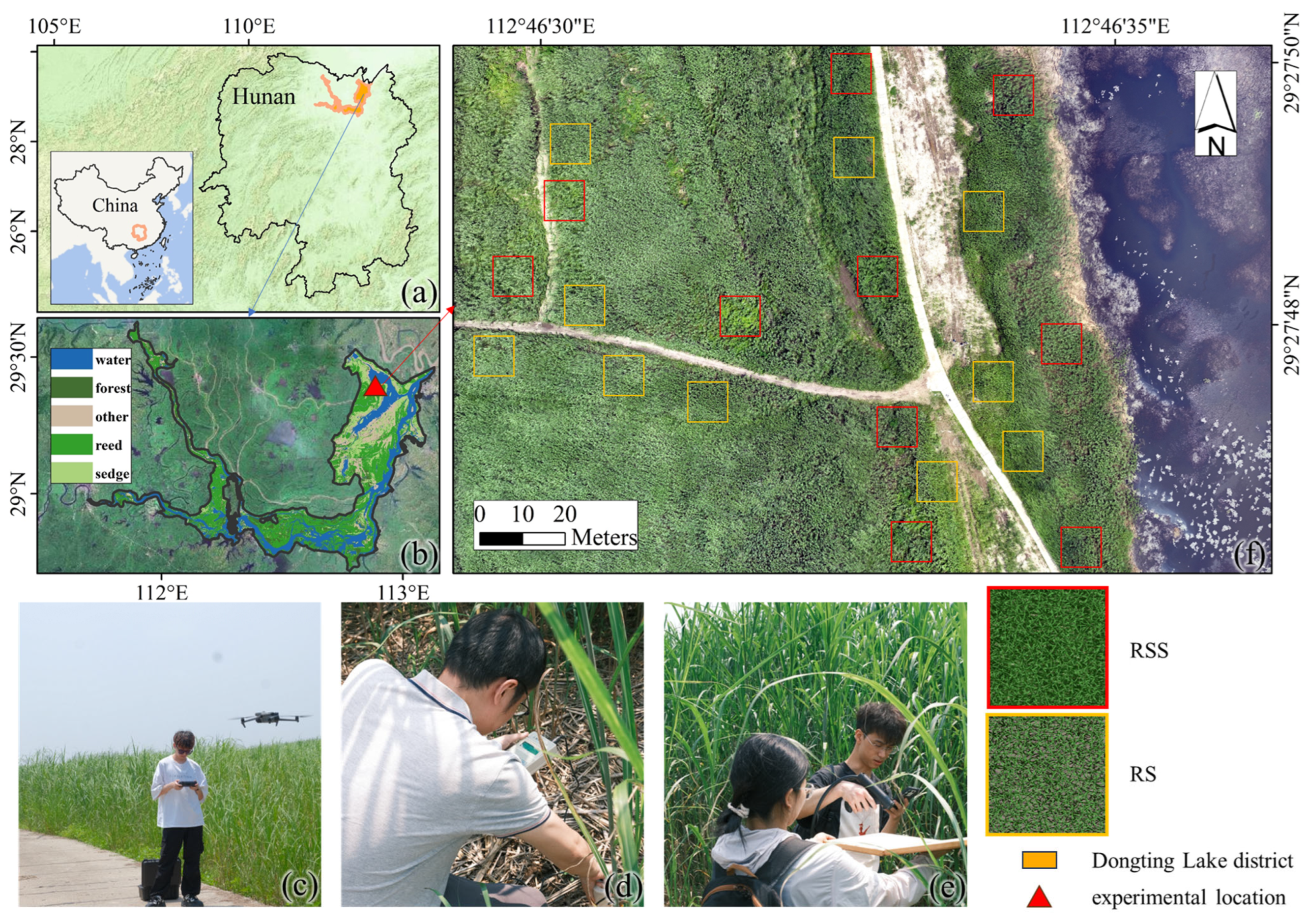
Figure 1. Overview of the study area. (a) Location of the study area. (b) Land cover maps (classified based on Sentinel-2 images) of the study area. (ce) Photographs of the field survey. (f) UAV image and plots in the experimental area. RS refers to the scene of reed monoculture, and RSS refers to the scene of mixed growth.
Remotesensing 17 03223 g001
Figure 2. Flowchart of the study.
Remotesensing 17 03223 g002
Figure 3. Optical properties of leaves and soils used in this study. For the green series, the solid line represents the reflectance and the dashed line represents the transmittance.
Remotesensing 17 03223 g003
Figure 4. The modeling process of the reed monoculture scene and the mixed-growth scene. In this study, individual reeds were evenly distributed in the scene to develop the reed monoculture scene in the wetland, and the mixed-growth scene, that is, the combination of one reed and one sedge plant, was evenly distributed in the scene.
Remotesensing 17 03223 g004
Figure 5. Two indicators used to evaluate VI saturation phenomena: (a) FPAR.inf and (b) FPAR.sat.
Remotesensing 17 03223 g005
Figure 6. Comparison of the reflectance simulated by LESS (Rsim) with reflectance observed by the HR-1024i and Sentinel-2 (Robs).
Remotesensing 17 03223 g006
Figure 7. Scatter plots between the Robs and Rsim.
Remotesensing 17 03223 g007
Figure 8. Comparison of the FPAR simulated by LESS (FPARsim) with FPAR observed by the SunScan canopy analysis system (FPARobs).
Remotesensing 17 03223 g008
Figure 9. The relationship between VIs and FPAR for RS.
Remotesensing 17 03223 g009
Figure 10. The relationship between VIs and FPAR for RSS.
Remotesensing 17 03223 g010
Figure 11. Effect of angle combination on the SD of VIs under different conditions; 1–12 refer to the 12 angle combinations.
Remotesensing 17 03223 g011
Figure 12. The level of impact of angle combinations on SD and reasons for changing the level of impact (the impact level of combinations on SD was not constant. For instance, when the soil condition is changed from W to F, the impact level of kNDVI changes from Q2 to Q1).
Remotesensing 17 03223 g012
Figure 13. FPAR.inf values in VIs in different scenes.
Remotesensing 17 03223 g013
Figure 14. FPAR.sat values in VIs in different scenes.
Remotesensing 17 03223 g014
Figure 15. FPAR.inf and FPAR.sat values in VIs for RS and RSS.
Remotesensing 17 03223 g015
Figure 16. Validation of FPAR predictions against GBOV ground truth data.
Remotesensing 17 03223 g016
Table 1. Input parameters for the LESS model.
CategoriesVariablesValues
CanopyPlant typeReed/sedge
Reed density (plants/m2)0–62
Competitive proportions1:1/pure reed
LeafCab (µg/cm2)20–50 for reed; 30 for sedge
N1.5 for reed and sedge
Carotenoids (µg/cm2)8 for reed; 0.7 for sedge
Water thickness (cm)0.012 for reed; 0.03 for sedge
Dry matter (g/cm2)0.007 for reed; 0.008 for sedge
EnvironmentSoil typeW/M/F
SZA:SAA (°)45:90/10:130/30:270
VZA:VAA (°)0:0/45:90/10:130/30:270
Terrain size (m)10 × 10 (Match the pixel size of Sentinel-2 image)
SensorTypePhoton tracing
Spectral bands (nm)400–900
Illumination resolution0.001
Productsbidirectional reflectance factor (BRF)/FPAR
Table 2. Computational formula of the selected 9 VIs. B, G, R, RE1, RE2, and NIR are the spectral bands of Sentinel-2.
VIsFormulaReference
GNDVI N I R G / N I R + G [39]
kNDVI tanh N D V I 2 [46]
RDVI ( N D V I × D V I ) [47]
SAVI N I R R / N I R + R + 0.5 × 1.5 [47]
NDVI N I R R / N I R + R [47]
DVI N I R R [47]
RVI N I R / R [23]
EVI 2.5 × N I R R / N I R + 6 R 7.5 B + 1 [48]
MTCI R E 2 R E 1 / R E 1 R [49]
Disclaimer/Publisher’s Note: The statements, opinions and data contained in all publications are solely those of the individual author(s) and contributor(s) and not of MDPI and/or the editor(s). MDPI and/or the editor(s) disclaim responsibility for any injury to people or property resulting from any ideas, methods, instructions or products referred to in the content.