Article

Driving Factors of Hala Lake Water Storage Changes from 2011 to 2023

by
Keyu Hu
1,†,
Longwei Xiang
1,2,*,†,
Hansheng Wang
3,
Holger Steffen
4,
Fan Deng
1,
Zugang Chen
2,
Guoqing Li
2,
Aile Nong
1,
Jingjing Guo
1 and
Xu Xiao
1
1
School of Geosciences, Yangtze University, Wuhan 430100, China
2
Aerospace Information Research Institute, Chinese Academy of Sciences, Beijing 100094, China
3
State Key Laboratory of Geodesy and Earth’s Dynamics, Innovation Academy for Precision Measurement Science and Technology, Chinese Academy of Sciences, Wuhan 430077, China
4
Geodetic Infrastructure, Lantmäteriet, 80182 Gävle, Sweden
*
Author to whom correspondence should be addressed.
These authors contributed equally to the work.
Remote Sens. 2025, 17(18), 3184; https://doi.org/10.3390/rs17183184
Submission received: 4 June 2025 / Revised: 8 September 2025 / Accepted: 9 September 2025 / Published: 14 September 2025

Abstract

Highlights

What are the main findings?
  • The lake area, water level, and LWSC of Hala Lake exhibited three stages of synchronous expansion from 2011 to 2023.
  • Lake surface precipitation and precipitation-caused runoff contributed the majority to the LWSC, with the latter being the key factor driving the formation of its three stages.
What is the implication of the main finding?
  • The study provides a practical and replicable blueprint for researching hydrological changes in alpine lakes and their responses to climate change.
  • The findings of this research offer useful insights for government agencies in the rational development and utilization of water resources.

Abstract

Monitoring the hydrological processes of lakes can provide reliable data for regional water resources assessment. This paper analyzed changes in the lake area and water level of Hala Lake from 2011 to 2023, subsequently estimating its lake water storage change (LWSC). We used image data from Landsat series satellites and multi-source satellite altimetry data, and then quantitatively assessed the influence of various driving factors on the LWSC in combination with hydrological and meteorological models. The results show three stages of parallel changes in the area, water level and LWSC of Hala Lake in the past 13 years. The first stage is from 2011 to 2014, when the lake expanded slightly, the second stage is from 2015 to 2019, when the lake expanded rapidly, and the last stage is from 2020 to 2023, with relatively stable conditions. Over the entire study period, the LWSC increased with a trend of 0.192 ± 0.009 km3/a. Lake surface precipitation, precipitation-caused runoff, and glacier meltwater contributed to the total recharge input by 51%, 40.96%, and 8.04%, respectively, while the lake surface evaporation accounted for 59.37% of the total recharge input as water loss. Thus, the left 40.63% of the input caused the LWSC increase. Although lake surface precipitation provided the primary contribution to the Hala Lake LWSC, precipitation-caused runoff was the key factor forming the three stages in the LWSC. The results of this study provide valuable information for the rational development and utilization of water resources by government departments and are also beneficial to the study of global change.

Graphical Abstract

1. Introduction

The Tibetan Plateau (TP) is known as the “Roof of the World” [1], with an average altitude of more than 4000 m, making it the highest and largest plateau in the world [2]. The TP contains numerous widely distributed lakes, with their total number and area accounting for about half of the total number and area of lakes in China. There are approximately 1400 lakes larger than 1 km2 in the TP, with a total area of 50,000 km2 [3,4]. The TP is extremely sensitive to climate change, and the temperature has risen significantly with global warming. Previous studies showed that the temperature on the TP increased at the rate of 0.37 °C/10a from 1961 to 2019, which was more than twice the global rate during the same period [5]. As the temperature rose, glaciers melted, which provided the potential sources of lake water recharges in the TP.
In the past decade, over 80% of the lakes on the TP expanded, and the expansion became more severe as the temperature rose [6]. Lake expansions can lead to disasters, such as the flooding of lake shore pastures, which impacted the regional ecological environment and the lives of farmers and livestock [7]. Lake water storage change (LWSC) reflects the regional water balance and hydrological cycles [8]; thus, obtaining real–time LWSC provides important data for regional water resources assessment, and is of great significance for regional ecological environment protection and comprehensive governance. However, the lack of field monitoring data on the TP severely hampers research progress on the LWSC in this region. The development of high-precision multi-temporal imaging and altimetry satellite technology has provided a large amount of data, based on which extensive studies have been conducted, investigating the LWSC on the TP. Yang et al. (2017) explored the LWSC of closed lakes larger than 50 km2 on the TP and their responses to climate change using the Shuttle Radar Topography Mission Digital Elevation Model (SRTM DEM) and Landsat imagery [9]. Zhang et al. (2021) analyzed changes in the area, water level, and LWSC of 25 typical lakes larger than 10 km2 in five regions on the TP from 1972 to 2019 based on the SRTM DEM and Landsat imagery, and also qualitatively analyzed the potential effects from temperature, precipitation, glacier melt, and permafrost degradation on the LWSC [10]. Similarly, combining satellite imagery and satellite altimetry, Sun et al. (2025) estimated the LWSC of Bangdag Co with lake area and water levels from 2010 to 2023 obtained from optical imagery and CryoSat–2 data, finding an increase of 1.04 km3 of the lake water [11]; Luo et al. (2021) estimated the LWSC of all lakes on the TP during 2003–2019, integrating the ICESat/ICESat–2, Global Surface Water dataset, and HydroLAKE dataset, and eventually came to an LWSC increase trend of 11.51 ± 2.26 Gt/yr [12]; and Chen et al. (2023) used Sentinel–3 to monitor four large lakes (Ayakkum Lake, Selinco Lake, Qinghai Lake, and Namco Lake) on the TP from April 2016 to September 2022, confirming that Sentinel–3 radar altimetry could accurately capture weekly and monthly lake level fluctuations, by comparison with in situ water level measurements and the DAHITI database [13]. In addition, exploring the relationship between the LWSC and its driving factors, Zheng et al. (2016) monitored changes in the water level, area, and water storage of Hulun Lake with Topex/Poseidon, Envisat RA–2 altimetry, and Landsat TM/ETM+ satellite imagery, and also investigated the correlation between lake changes and climatic change [14]. Yang et al. (2020) used MODIS images to extract the area of the Aral Sea with the Normalized Difference Vegetation Index (NDVI), calculated the LWSC, and analyzed the effects of precipitation, glacier meltwater, and human activities on the LWSC [15]. These studies demonstrated that using satellite imagery and satellite altimetry can effectively monitor the LWSC for lakes, especially for lakes on the TP that lack field observations, and that the driving factors of the LWSC can also be investigated in combination with hydrological and meteorological models and observations.
Located in the northeastern part of the TP, the Hala Lake basin is a typical endorheic basin, which has a temperate continental climate, with an average annual temperature of 5.9   ° C , and annual precipitation of 250–300 mm [16]. Li et al. (2019) found that most of the hydrological changes in the Hala Lake resulted from the precipitation in the basin and the meltwater from the glacier covering the surrounding mountains [17]. Glaciers and permafrost are widely distributed in and around the basin, making it extremely sensitive to climate change, while the impact of human activities is weak here. This makes the basin an ideal choice for investigating how the hydrological changes there are connected to climate change.
Most previous studies focused on the geological structure in the basin and/or lake sediments [18,19,20,21]. There are also studies that referred to the changes in the area, lake level, and LWSC of Hala Lake, as well as the potential effects from climate change. Li et al. (2021) investigated the area changes of Hala Lake from 1986 to 2015 based on Landsat images, showing an increasing trend since 2001 just after a long declining period, and analyzed its response to climate change, finding precipitation to be the dominant driving factor [22]. Wang et al. (2021) [23] analyzed interdecadal, interannual, and intra-annual changes in Hala Lake’s area (1986–2019) and their drivers, using multi-source satellite and meteorological data. Consistent with the study of Li et al. (2021) [22], Wang et al. (2021) also found 2001 as the turning point, shifting the lake from a decline to an increase, and that lake water changes were linked to climate change and glacial retreat, with precipitation as the dominant factor [23]. However, these two studies only analyzed Hala Lake area changes and did not provide further insight into the lake level or even LWSC. Wu et al. (2016) extracted Hala Lake levels and areas based on altimetry data and Landsat images from 2000 to 2015, and analyzed the effects of glaciers melting and precipitation, but did not quantitatively analyze the effects of evaporation, which caused most lake water loss [24]. Based on the GEE platform and meteorological data, Jiang et al. (2022) studied the feedback of the LWSC on climate change in the Hala Lake basin from 1987 to 2018 [25]; however, they only obtained ICESat1/2 lake level data from 2003 to 2009 and the year 2018. Given the limited measured water levels used for function fitting, the resulting lake level data inevitably had lower reliability, especially for the years from 2009 to 2018.
In this study, we integrated multi-source datasets from 2011 to 2023, including Landsat series imagery, multi-platform satellite altimetry, and multiple hydrological and meteorological models, to accurately calculate the monthly LWSC of Hala Lake, which yielded a higher temporal resolution than that provided by previous studies on Hala Lake. This enabled us to reveal the spatiotemporal variation characteristics of the LWSC, and quantitatively analyze the impacts of lake surface precipitation ( P L ), evaporation ( E L ) , precipitation-caused runoff ( R P ), and glacier meltwater ( G ) on the LWSC. Furthermore, we analyzed the connection between the LWSC of Hala Lake and climate change. The results of this study will provide local departments with a theoretical basis and reliable data for the comprehensive management of the ecological environment, as well as the rational development and utilization of water resources.

2. Data and Methods

2.1. Study Area

The Hala Lake basin is a complete and independent small endorheic basin of about 4801 km2 (Figure 1). Its maximum east–west length is about 120 km, and the utmost north–south width is about 78 km. The southern edge is Halco Mountain, while the northern edge is Shule South Mountain with the 5808 m high Gangze Wujie Peak [24]. Hala Lake, the second-largest lake in the Province of Qinghai, is an approximately oval-shaped large saltwater lake at an elevation of about 4078 m, with a length of about 34.2 km, and a width of about 23.0 km; thus, its area is about 637 km2 [23]. The glaciers around the Hala Lake basin are mainly distributed in the Shule South and Halco mountains (Figure 1). According to the Second Chinese Glacier Inventory, there are 118 glaciers in the basin, 70 glaciers in Shule South Mountain, and 48 glaciers in Halco Mountain. The largest glacier is the Gangnalou Glacier in the Shule South Mountain [26]. There are more than 20 rivers, most of which are seasonal rivers, supplying the lake water. The water system is centripetal, converging the surface and subsurface runoffs to the lowest part of the basin where Hala Lake lies. The LWSC is mainly affected by climate change, in the form of replenishment from precipitation and glaciers melting with significant seasonal variation [16], while lake water loss is mainly due to evaporation.

2.2. Data

2.2.1. Landsat Satellite Imagery

We extracted the Hala Lake boundary from 2011 to 2023 using multi–spectral and multi–temporal imagery from Landsat 5, 7, 8, and 9 satellites. The Landsat images used were all Level 2 data processed by systematic radiometric calibration and atmospheric correction. The Hala Lake basin covers two Landsat scenes which were spliced together, and in total, 105 cloudless images of the basin were collected from 2011 to 2023 (Table 1).

2.2.2. Satellite Altimetry

Altimetry data from CryoSat–2, Sentinel–3, and ICESat–2 satellites were used to monitor the changes of the lake water level in this study.
The CryoSat–2 was launched in April 2010, equipped with an advanced synthetic aperture interferometric radar altimeter, which operates in three distinct modes: the Low Resolution Mode (LRM), Synthetic Aperture Radar Mode (SAR), and Synthetic Aperture Radar Interferometric Mode (SARIn) [27]. CryoSat–2 has a repetition period of 369 days and a sub–period of 30 days, providing a high spatial coverage of 30 m on the ground [28]. Geophysical corrections have been used in the CryoSat–2 Level 2 data to correct altimeter measurements from different perturbations [29]. In areas with complex topography, such as the TP, CryoSat–2 operated in the SARIn mode, which was designed to obtain elevations of variable terrain [30].
Sentinel–3 is a European Earth observation satellite mission that supports monitoring and research applications in the ocean, land, atmosphere, and cryosphere [31]. Launched in 2016 with a 27–day revisit period, the Sentinel–3A satellite carries an SRAL (SAR Radar ALtimeter) and is capable of emitting microwaves in the Ku band for ranging and in the C band for determining ionospheric errors [32]. We used Sentinel–3A SRAL L2 data from June 2016 to the present, with 338 altimeter transit tracks and 68 effective elevation points.
ICESat–2 is an altimetry satellite launched by the National Aeronautics and Space Administration (NASA) in September 2018 with a revisit period of 91 days [33]. It is equipped with an advanced topographic laser altimeter system (ATLAS), which consists of a multi–beam, micropulse, low-energy, high-resolution, photon-counting laser altimeter, with three pairs of beams, each spaced approximately 3 km apart across orbits, and 90 m apart along the orbit [34]. Each beam has a nominal diameter of 17 m and a sampling interval of 0.7 m along the orbit [35]. ICESat–2/ATL13 (v6) data were used in this study, covering the period from October 2018 to December 2023.

2.2.3. Hydrological and Climatic Data

To analyze the monitoring results of the LWSC in Hala Lake and their corresponding driving factors, we employed multiple hydrological and climate models and used different analysis methods. The Hydroweb datasets [36] provided by the French Center for Geophysics and Oceanography Space Observation and Research were selected to check the extracted lake levels and areas of Hala Lake.
The ‘1–km monthly precipitation dataset for China (1901–2023)’ [37] was chosen for the precipitation analysis, while the ‘Evaporation dataset of the Tibetan Plateau at the monthly scale (1979–2018) V2.0’ [38] and the ‘1–km monthly potential evapotranspiration dataset for China (1901–2023)’ [39] were selected for the evaporation analysis.
Other climatic data such as air temperature, ground temperature, and hydrological data of soil moisture (SM) were retrieved from NASA’s Global Land Surface Data Assimilation System (GLDAS) model [40].

2.3. Methods

2.3.1. Extraction of the Lake Area

At present, methods for lake area extraction from multi–spectral remote sensing images include single–band density slicing, supervised or unsupervised classification, water index, etc. [41], among which the water index is mostly used because of its simple form and easy to use [42]. In this study, the normalized difference water index (NDWI) [43] was used to extract Hala Lake areas from 2011 to 2023, with the following equation:
N D W I = b a n d g r e e n b a n d n i r b a n d g r e e n + b a n d n i r ,
where b a n d g r e e n is the reflectance of the green band; b a n d n i r is the reflectance of the near infrared (NIR) band. The threshold for extracting the Hala Lake area here is selected manually, and the justification using Hydroweb data will be shown below.
Due to the influence of natural events, such as flying clouds blocking and winter snow covering, it was hard to obtain lake areas for all months during the study period based on satellite imagery, and therefore, two methods were used to supplement the missing monthly lake areas in this study. One method calculated the missing lake area by stage fitting, since lake area changes periodically. Due to the influence of seasonal precipitation and evaporation, and seasonal meltwater from glacier, the fluctuation of lake water was often drastic in a year. Previous studies showed that lake water on the TP decreased from January to April or May, then increased and reached its maximum in August, followed by another decrease, with another trough in April or May in the next year [44,45]. Thus, the pattern of lake water changes within a single year or between two consecutive years can be seen as a ‘decrease–increase–decrease’ or ‘increase–decrease–increase’, respectively, which can be mathematically represented by a third-degree polynomial function. Therefore, we employed this type of function in a stage fitting approach to supplement the missing monthly Hala Lake areas from 2011 to 2023.
The other method estimates the missing lake area by the lake level–area relationship, establishing specific functional relationships between the lake levels and areas. A large number of studies confirmed the applicability and reliability of this method [46,47]. Currently, polynomial function, exponential function, and power function can all be used to simulate the lake level–area relationship [48,49]; therefore, the three types of function models were used to find the optimal lake level–area relationship in this study.

2.3.2. Calculation of the Lake Level

The elevation of the lake surface, also referred to as the lake water level, can be obtained from satellite altimetry data. The average elevation of the altimetry footprint points for one observation that are scattered within the lake were used to represent the lake water level. Certainly, the corresponding transforms and error correction are inevitable, which can be implemented with the following [50]:
H = A l t R a n g e H c o r G e o i d ,
H c o r = δ d r y + δ w e t + δ i o n o + δ s o l i d + δ p o l e ,
where in Equation (2), H is the distance from the lake surface to the geoid (m), A l t is the distance from the satellite to the reference ellipsoid (WGS84) (m), R a n g e is the distance from the satellite to the measured lake surface (estimated with the waveform retracking algorithm) (m), H c o r is the error correction (m), and G e o i d is the height between the reference ellipsoid (WGS84) and the geoid (EGM2008) (m). In Equation (3), δ d r y , δ w e t , δ i o n o , δ s o l i d , and δ p o l e correspond to the corrections for the dry troposphere, the wet troposphere, the ionosphere, the solid earth tide, and the pole tide, respectively. Note that the G e o i d referred to here represents the height relative to the different geoid models used for different satellite altimetry data: the EGM96 model for CryoSat–2 and the EGM2008 model for Sentinel–3 and ICESat–2. For consistency, the G e o i d for CryoSat–2 was converted to EGM2008 here.
Due to the errors in lake boundary extraction and echo anomaly, outliers often occurred in the observed lake water levels, which needed to be eliminated for accurate lake water level simulation [13]. We applied the K–means clustering method [51] and the boxplot method [52] to remove the outliers. Concretely, based on the optimal class determined by K–means clustering, the upper and lower thresholds [53] were given by Equations (4) and (5) below, beyond which the outliers were excluded, as follows:
Q u p = Q 1 + 1.5 × c ,
Q l w = Q 2 1.5 × c ,
where Q u p and Q l w are the upper and lower thresholds, Q 1 and Q 2 are the upper and lower quartiles, while c is the difference between the upper and lower quartiles, i.e., ( Q 1 Q 2 ).
Since we have selected three types of altimetry satellite data, it is necessary to remove the systematic errors between different datasets. Although deviations occur among altimetry data from different satellites, the accuracy of laser altimetry is usually higher than that of radar altimetry [54]. Therefore, after excluding the outliers, we used ICESat–2 lake levels as the reference to calculate the average bias between CryoSat–2 or Sentinel–3 lake levels and ICESat–2 lake levels, respectively. Then, the CryoSat–2 and Sentinel–3 levels were adjusted by subtracting the average biases normalizing CryoSat–2 and Sentinel–3 lake levels with the following:
H c a l i b i = H i + H b i a s ,
H b i a s = i = 1 n ( H I C E S a t 2 i H ( i ) ) n ,
where H c a l i b i is the calibrated lake water levels at time i , H i is the lake level to be calibrated (observed by either CryoSat–2 or Sentinel–3) at time i , while H b i a s is the average deviation between H ( i ) and H I C E S a t 2 i , which is the reference lake levels by ICESat–2, while n is the number of the involved deviations. Lastly, the average of the lake water levels at the same month was recognized as the monthly Hala Lake water level.
In this study, CryoSat–2 provided Hala Lake water level data for most of the months from 2011 to 2023, Sentinel–3 covered the observation period from June 2016 to December 2023, and ICESat–2 provided data from 2018 to 2023; however, missing monthly elevations occurred in the missions’ data. We used two methods to supplement the missing monthly lake water levels: stage fitting with a third-degree polynomial function, and the lake level–area relationship. Finally, the average was taken as the final monthly lake water level where the satellite altimetry data overlapped.

2.3.3. Estimation of Lake Water Storage Changes

Closely related to the changes in lake levels and areas, the Hala Lake LWSC can be estimated by the following [55]:
V i , j = 1 3 × H i , j × ( A i + A j + A i × A j ) ,
where V i , j is the LWSC (km3) between time i and j , A i and A j are the lake areas at time i and j , respectively, while H i , j is the lake level change from time i to j .

2.3.4. Estimation of Glacier Meltwater

Previous studies have shown that the glacier area on the TP decreased over the past few decades, and glacier meltwater flowed into the lakes, resulting in the LWSC [56]. Due to the fact that the severe melting of glaciers usually occurred in a high-temperature summer, we chose clear Landsat images with no or few clouds in summer to extract the glacier area based on the Normalized Difference Snow Index (NDSI) [57].
N D S I = b a n d g r e e n b a n d s w i r b a n d g r e e n + b a n d s w i r ,
where b a n d g r e e n is the reflectance of the green band, and b a n d s w i r is the reflectance of the shortwave infrared (SWIR) band. Note that the glacier area referenced here includes the area of glaciers with their covering snow.
Liu et al. (2003) proposed the empirical formula below for estimating glacier volume changes in the Qilian Mountains region including the Hala Lake basin, and verified its validity with various in situ measurements [58]; therefore, we used it in estimating glacier volume changes in this study, as follows:
V g = 0.04 × S 1.35 ,
where V g is the volume of the mountain glacier (km3) and S is the glacier area (km2).
Assuming that the glacier meltwater would eventually flow into Hala Lake, the meltwater amount can be converted from glacier volume changes with the following:
G i , j = ρ 1   ×   ( V g i V g j ) ρ 2 ,
where G i , j represents the glacier meltwater (km3) between time i and j , V g i and V g j are the volume (km3) of glacier at time i and j , while ρ 1 and ρ 2 are the density of ice (0.85   ×   103 kg/m3) and water (1.0   ×   103 kg/m3), respectively.

2.3.5. Simulation of Lake Water Storage Changes

There are two forms of water recharge input into Hala Lake: one is the direct input from lake surface precipitation and the other is runoff, which is mainly formed by land precipitation and glacier meltwater, and may also include a small amount formed by permafrost degradation and groundwater changes. However, as an endorheic lake, the water loss of Hala Lake is mainly caused by evaporation. Therefore, from the perspective of lake water balance, we can also simulate Hala Lake LWSC, which we abbreviate to ‘simulated LWSC’, which corresponds to the previous LWSC obtained by satellite monitoring, abbreviated to ‘monitored LWSC’. The simulated LWSC (∆V) can be expressed as follows:
V = P L E L + R P + G ,
where P L and E L are the lake surface precipitation and evaporation, respectively; R P is the precipitation-caused runoff considering soil moisture, which is simply defined by land precipitation deducting land evaporation as well as the moisture changes in the soil; and G is the glacier meltwater. The evaporation data here (including lake surface evaporation and land evaporation) have been processed (Appendix A.1). Note that the effects of permafrost degradation and groundwater storage changes on the simulated LWSC were not included here due to a lack of reliable observations or models. However, the simulated LWSC can be cross-validated with the aforementioned monitored LWSC, for instance, by means of the Pearson’s correlation coefficient [59] (Appendix A.2).

2.4. Uncertainty Assessment

2.4.1. Uncertainty of Lake Water Storage Change

Based on the error propagation law, the errors of the monthly simulated LWSC can be calculated as follows [25]:
  σ V i , j = 1 3 × A i + A j + A i × A j × σ H i , j 2 + H i , j + H i , j × A j 2 × A i × A j 2 × σ A i 2 + H i , j + H i , j × A j 2 × A i × A j 2 × σ A j 2 ,
where σ V i , j is the error of the simulated LWSC between times i and j , σ H i , j = 2 × L T L r is the error of the lake level changes between elevations at times i and j , where L is the deviation vector between the satellite altimetry data and the corresponding fitted data, while r is the number of data values. σ A i and σ A j are the lake area errors, determined by 0.198 % × A i / j , where the scale factor 0.198% was given by the relative deviation between the extracted lake areas and those from Hydroweb datasets. Given the errors of the monthly simulated LWSC, the error of the simulated LWSC over a specific time span can be estimated using the law of error propagation. Finally, we took twice the errors as the uncertainties.

2.4.2. Uncertainty of Glacier Meltwater

Glacier meltwater was obtained through an empirical formula with glacier areas. The glacier area error here refers to that caused by the resolution of satellite image data, which can be calculated through multiplying the number of pixels at the glacier edge by half the area of a single pixel [60], as follows:
σ S G = N   × S h a l f ,
where σ S G is the glacier area error (km2), N   is the number of pixels at the glacier edge in the image, and S h a l f   stands for the half area of a single pixel (for Landsat TM/ETM+/OLI images, S h a l f = 0.45 × 10⁻³ km2).
Based on Equation (10), the glacier volume changes error ( σ V G ) can be derived using the law of error propagation:
  σ V G = 0.054 × σ S G 0.35 ,
And consequently, glaciers meltwater errors ( σ G i , j ) can be estimated according to Equation (11), as follows:
  σ G i , j = 0.85 × σ V G i 2 + σ V G j 2 ,
where σ V G i and σ V G j are the glacier volume errors (km3) at times i and j . Again, we took twice the errors as the corresponding uncertainties.

2.4.3. Uncertainty of Estimated Hydrological and Climatic Contributions

We used models to simulate the LWSC based on hydrological and climatic contributions using Equation (12). The errors of these contributions at different stages can be calculated by the Root Mean Square Error (RMSE). As before we took twice the errors as uncertainties.

3. Results

3.1. Changes in Hala Lake Area, Lake Level, and Lake Water Storage

Due to the missing data, it is difficult to obtain a complete lake area and lake level changes time series for Hala Lake only by satellite altimetry and imagery. As mentioned above, two methods of stage fitting and lake level–area relationship were used to supplement the missing monthly lake areas and levels during the study period in this study, and two statistical indicators of RMSE and Coefficient of Determination (R2) were introduced (Appendix A.3) to evaluate their credibility. The larger the R2 and the smaller the RMSE are, the higher the fitting accuracy is, and vice versa.
For the stage fitting method, the third-degree polynomial function was eventually taken, as indicated by the large R2 and small RMSE (Table A3 and Table A4). For the lake level–area relationship method, we tested in total 13 fitting formulas (9 polynomial functions, 2 exponential functions, and 2 power functions), as shown in Table A5 and Table A6. We found that the seventh-degree polynomial function best described the relationship between the lake area and lake level. It yielded the highest R2 and the lowest RMSE, indicating a higher fitting accuracy than other functions.
The complete lake areas supplemented through stage fitting and the lake level–area relationship show excellent agreement (Figure 2). In view of their high similarity, the average was used as the reliable monthly lake area changes. Figure 2 shows that the Hala Lake area increased with a trend rate of 3.544 ± 0.169 km2/a over the past decade. In February 2011, the lake area reached its lowest value of 603.503 ± 2.393 km2, and then increased to 641.527 ± 3.158 km2 in 2021.
Similarly, the complete lake levels supplemented through stage fitting and the lake level–area relationship also show strong consistency (Figure 2). The average was finally taken for the lake level changes. Similar to the changes in lake areas, the analogous variations occurred in lake water levels, which exhibited an increasing trend of 0.308 ± 0.014 m/a throughout the study period. The lowest lake level of 4078.683 ± 0.113 m was reached in February 2011, which then began to increase, reaching 4082.011 ± 0.593 m in 2021.
Carefully examining the area and level changing curves, the same pattern of three stages can be distinguished in each curve, with 2015 and 2020 being the turning years (Figure 2). There is first a slight increase stage from 2011 to 2014, with trends of 1.151 ± 0.320 km2/a for area increase and 0.093 ± 0.036 m/a for lake level increase. This is followed by a rapid increase stage during 2015 and 2019, with trends of 5.646 ± 0.482 km2/a and 0.497 ± 0.035 m/a, respectively. Finally, a stable stage occurs between 2020 and 2023, with only subtle trends of 0.102 ± 0.304 km2/a and 0.027 ± 0.029 m/a, respectively. Note that the uncertainties are larger than the trends themselves in the stable stage.
The three stages can also be seen in the monitored LWSC. The overall trend rate of 0.192 ± 0.009 km3/a during 2011 and 2023 (Figure 2) can be subdivided into a slight increase trend of 0.056 ± 0.022 km3/a from 2011 to 2014, followed by a rapid increase trend of 0.308 ± 0.022 km3/a during 2015 and 2019, and then a stable trend between 2020 and 2023, with a subtle trend of 0.017 ± 0.018 km3/a. A bar chart of the monthly monitored LWSC is also shown in Figure 2, which shows a more positive monthly LWSC than negative ones during 2015 and 2019, leading to the rapid increase stage. A similar behavior can be seen from 2011 to 2014, but with a bit less positive monthly LWSC, which caused the slight increase trend. The bars are nearly balanced for the monthly LWSC between 2020 and 2023. For all stages, the positive monthly LWSC usually happened in summer due to much heavier precipitation than evaporation, while the negative ones occurred more often in late autumn or early winter because of stronger evaporation than precipitation, with the largest monthly increase of 0.328 ± 0.017 km3 in July 2023, and the strongest monthly decline of −0.253 ± 0.015 km3 in December 2022.

3.2. Simulation of Hala Lake Water Balance

The LWSC acts as a link between surface hydrological processes and climate change. Climatic driving factors, such as changes in precipitation, evaporation, and temperature, can lead to water recharging input and water losing output of the Hala Lake basin, and ultimately exert a substantial influence on the LWSC [61,62,63].

3.2.1. Hala Lake Water Storage Changes Response to Climate Change

Generally, higher precipitation than evaporation in summer results in increasing water storage in the Hala Lake basin, while lower precipitation than (or equal to) evaporation in other seasons leads to decreasing or stable water storage. The net precipitation (NeP), defined as precipitation minus evaporation, usually matches the LWSC in the basin.
From 2011 to 2023, the NeP in the Hala Lake basin matched the yearly monitored LWSC, with a high Pearson’s correlation coefficient of 0.77 (Figure 3). Three stages were also found in the yearly monitored LWSC, among which the average yearly changes are 0.072 ± 0.017 km3, 0.304 ± 0.017 km3, and 0.057 ± 0.021 km3 for the three periods of 2011–2014, 2015–2019, and 2020–2023, respectively. Acting as the driving factor, NeP shows stable, rapid growth and slight reduction stages, with an average yearly NeP of −0.006 ± 0.272 km3, 0.196 ± 0.225 km3, and −0.215 ± 0.181 km3, respectively for the three periods. Although there is a high correlation between the yearly NeP and yearly monitored LWSC, it is worth noting that the LWSC is also influenced by meltwater from glacier melting. Considering this, the simulated LWSC derived from the lake water balance method should show improved consistency with the monitored LWSC by satellite altimetry and imagery.
Combining monthly air temperature and NeP data, Figure 3 clearly shows that the LWSC starts to increase from middle spring or early summer in April to June when the precipitation starts to increase and evaporation is relatively weak as the air temperature is low, thus leading to a positive NeP. The LWSC peaks between May and July, despite the high temperatures or even negative monthly NeP. This is possibly mainly due to the surface and underground runoff caused by land NeP and glacier melting when the air temperature rises above 0 °C. After that peak, the LWSC decreases because of strong evaporation and the gradually decreasing precipitation in autumn and winter.

3.2.2. Simulation of Glacier Melting

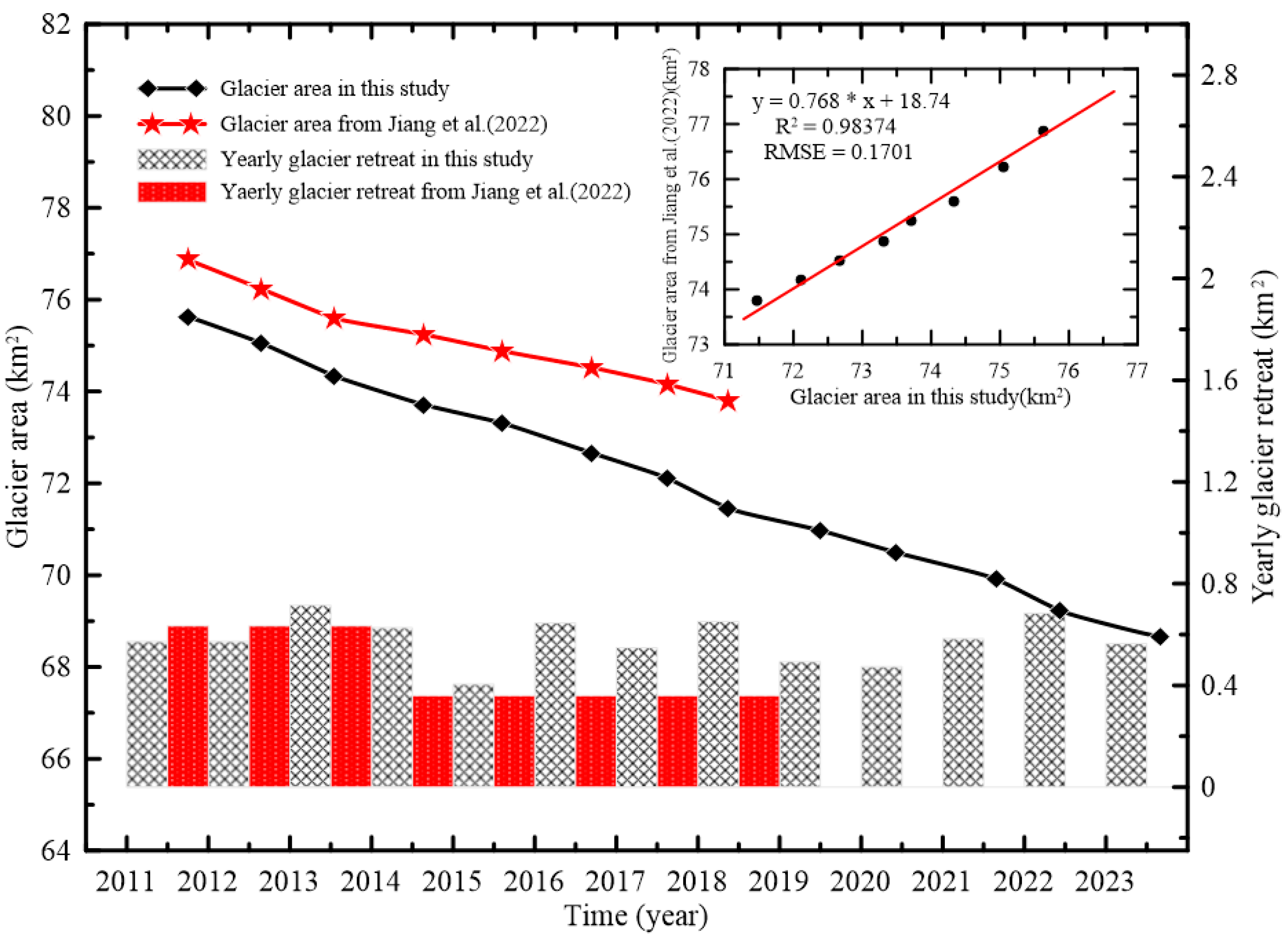
For endorheic lakes such as Hala Lake, meltwater from glaciers is an important source of lake water recharge besides the NeP. Due to global warming, glaciers melt with their surfaces thinning and their edges retreating. As shown in Figure A3, the Gangnalou Glacier and its surrounding glaciers exhibited evident retreat in the northern part of the basin. Based on Landsat imagery, we found that the area of glaciers in the basin decreased from 75.626 ± 13.736 km2 to 68.664 ± 11.120 km2 from 2011 to 2023, with an average rate of 0.536 ± 1.359 km2/a.
Exploring the relationship between glacier melting and summer air temperature changes, we found that glacier melting matched the summer air temperature change well (Figure 4). Summer air temperature changes directly affected the glacier surface area: higher temperatures accelerated glacier melting, producing more meltwater, while lower summer air temperatures led to less meltwater. Although we estimated the meltwater using Equations (9)–(11), with no reliance on air temperature changes, the resulting meltwater curve exhibits a variation pattern that aligns with that of the summer air temperature curve. The meltwater volume in 2013 was the highest, at approximately 0.149 ± 0.264 km3, which corresponds to the highest summer air temperature of 7.069 °C; in contrast, the lowest meltwater volume (0.084 ± 0.254 km3) occurred in 2015, associated with the lowest summer air temperature of 4.539 °C (Figure 4). From 2011 to 2023, the total amount of glacier meltwater volume in the Hala Lake basin was 1.548 ± 0.263 km3, with a yearly average of 0.119 ± 0.020 km3. Corresponding to the three periods of 2011–2014, 2015–2019, and 2020–2023, the yearly averages were 0.129 ± 0.068 km3, 0.113 ± 0.053 km3, and 0.117 ± 0.064 km3, respectively.

3.3. Water Balance of Hala Lake

Hala Lake LWSC is caused by the combination of hydrometeorological factors [25]. Precipitation, evaporation, soil moisture, and glacier melting were considered in this study to simulate the LWSC by the lake water balance of Equation (12), which was then compared with the monitored LWSC from satellite observations.
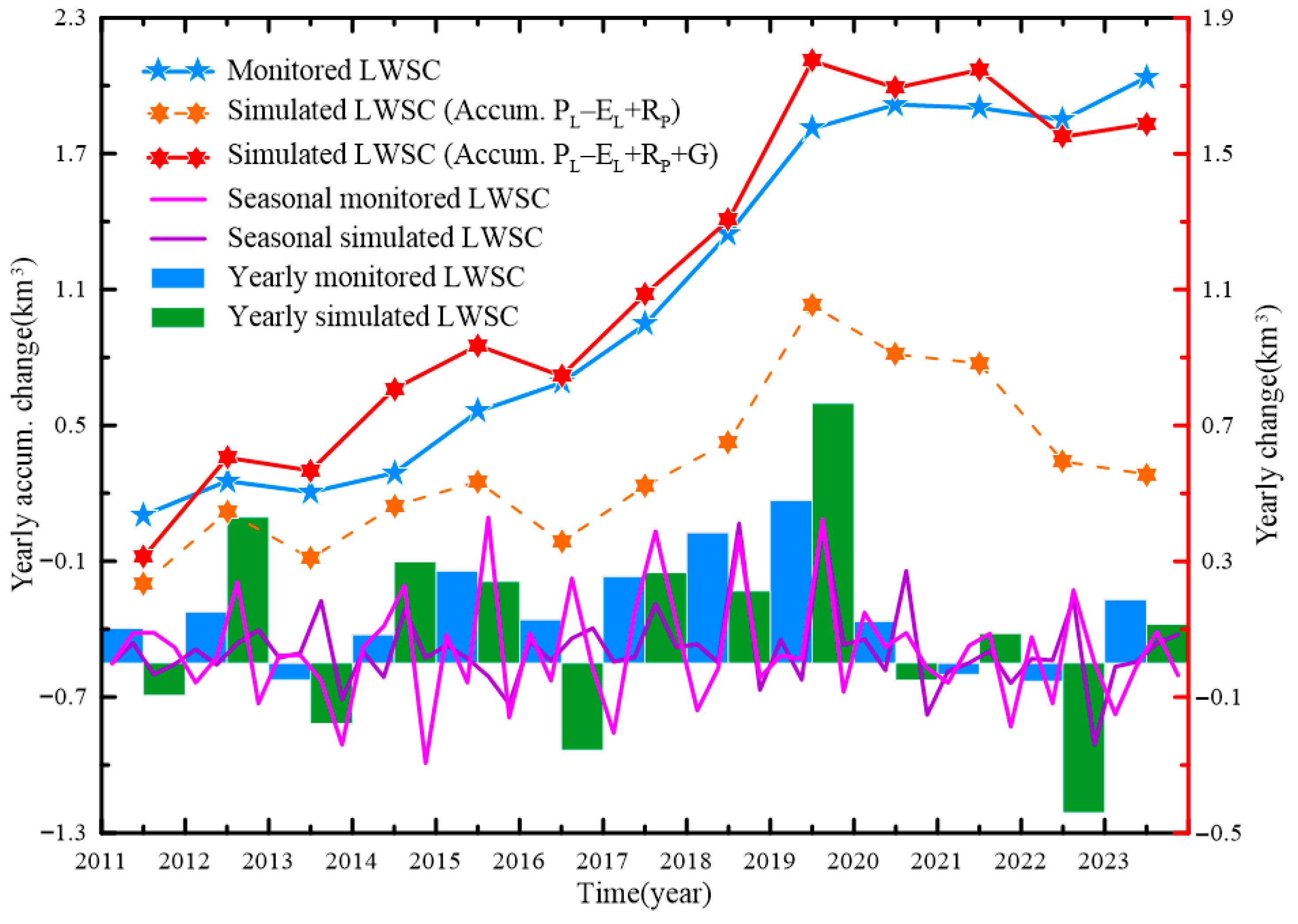
The LWSC was influenced by multiple factors, among which, lake surface precipitation ( P L ) and evaporation ( E L ), precipitation-caused runoff ( R P ), and glacier meltwater (G) were the key factors. Figure 5 shows that the simulated LWSC was significantly lower than the monitored LWSC when the glacier meltwater was not considered. However, when the glacier meltwater was included, the simulated LWSC was in good agreement with the monitored LWSC, with the Pearson’s correlation coefficient to be 0.973. Despite that, larger differences occurred in some years, such as in 2014, 2015, and 2019. The results further showed that the seasonal simulated LWSC matched the seasonal monitored results, with a correlation coefficient of 0.536, and the simulated yearly LWSC was also consistent with the monitored results, with a Pearson’s correlation coefficient of 0.742.
In conclusion, P L , R P , and G recharge for LWSC, while E L was the main output. These main hydrological and meteorological factors collectively drove the hydrodynamic balance of water storage in Hala Lake.
Quantifying the contributions of each input and output term in Equation (12), the results are summarized in Table 2. For the slight increase stage from 2011 to 2014, the average yearly changes of P L was 0.173 ± 0.026 km3, while those of R P , G , and E L were 0.177   ±   0.218 km3, 0.021   ±   0.015 km3, and 0.206   ±   0.011 km3 (output), respectively. For the rapid increase stage during 2015 and 2019, the average yearly changes of P L , R P , G , and E L were 0.194 ± 0.028 km3, 0.256 ± 0.210 km3, 0.038 ± 0.035 km3, and 0.199 ± 0.013 km3 (output), respectively, which showed that the rapid increase stage was caused by increased recharges, especially the significant growth of R P . For the stable stage between 2020 and 2023, the corresponding average yearly changes were 0.159 ± 0.020 km3, −0.036 ± 0.131 km3, 0.022 ± 0.018 km3, and 0.215 ± 0.014 km3 (output), respectively, in which the significant drop in R P altered the curves’ trajectory, while the other variables remained relatively stable. Therefore, the variations in P L , R P , G , and E L collectively drove the Hala Lake LWSC, while the significant increases or drops in R P were the primary cause of the three stages.
Over the entire study period from 2011 to 2023, the average yearly P L amounted to 0.177 ± 0.015 km3, while the average yearly R P and G were approximately 0.142 ± 0.112 km3 and 0.028 ± 0.015 km3, respectively. In contrast, the average yearly water loss via E L was about 0.206 ± 0.007 km3, and consequently, Hala Lake exhibited a distinct increase in the LWSC (Figure 5). Calculating the contribution of each component to the total recharge input during the study period, the mean yearly contribution of P L , R P , and G   were 51%, 40.96%, and 8.04%, which recharged Hala Lake. Conversely, the water loss induced by E L represented 59.37% of the total recharge input. Deducting the water loss from all the total recharge input, we got the LWSC of Hala Lake. Note that although the R P was the key factor forming the three stages of the LWSC, the P L was the primary contribution in maintaining the LWSC, while G provided the lowest but indispensable contribution.

4. Discussion

4.1. Comparison with Previous Studies

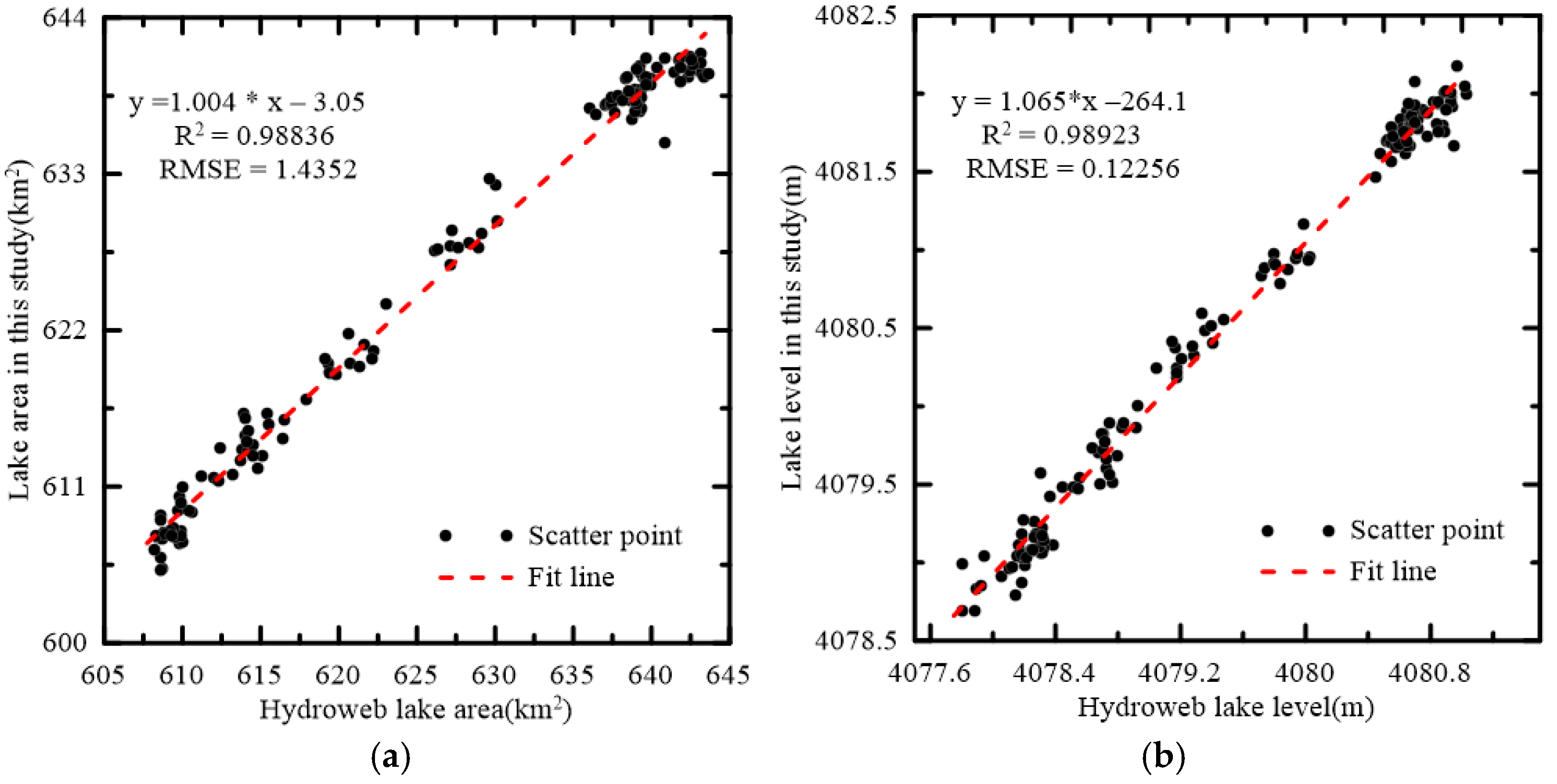
To verify the lake level and area changes obtained by satellite observation in this study, we compare our results with those from Hydroweb using two statistical indices R2 and RMSE (Figure 6). The results show that the R2 and RMSE for the lake area were about 0.988 and 1.435, respectively, while those for lake levels were about 0.989 and 0.123, respectively. This proved the reliability of our results.
When comparing our glacier melting simulation results with those of previous studies (Figure 7), we found that our results regarding glacier area changes are consistent with those of Jiang et al. (2022) [25], with an R2 and RMSE of 0.984 and 0.170, respectively. However, compared with Jiang et al. (2022) [25], we used more images in this study: specifically, at least one clear, cloud–free, or low–cloud Landsat image acquired in summer each year was used to extract glacier area. Evidently, the use of more images enhances the reliability of the glacier retreat results.

4.2. Other Factors Introducing Uncertainty

Uncertainties in the monitored LWSC results of this study are related to the limited resolution of Landsat images, inherent limitations of water indices, and clouds/snow covers, all of which introduced errors during lake area extraction. Additionally, there are waveform retracking errors in radar altimetry and inter-dataset systematic biases in altimetry data, which caused errors in water level acquisition. Furthermore, due to the lack of field observations, it is difficult to effectively estimate the impact of permafrost degradation and groundwater changes on the simulated LWSC. Moreover, potential underground leakage through the fault zones [21] may reduce Hala Lake’s LWSC, which we cannot account for due to missing data. As a result, inevitable data processing errors and the omission of certain water recharge sources resulted in additional discrepancies between our results and the actual water volume changes.

4.3. Perspective of the Hala Lake Water Balance

As stated above, lake surface precipitation, precipitation-caused runoff, and glacier meltwater contributed to the rapid expansion of Hala Lake water storage. Among these recharge components, P L and R P accounted for the majority (Table 2). This finding is also supported by Lei and Yang (2017) [62]. According to previous studies, the climate of the TP will be warmer and wetter in the 21st century, which will lead to an increase in precipitation and NeP, by projections based on the IPCC AR6–assessed likely range of equilibrium climate sensitivity (ECS), and the Coupled Model Intercomparison Project Phase 6 (CMIP6), under Shared Socioeconomic Pathway (SSP) scenarios [64,65,66]. Therefore, it is reasonable to infer that under this climate change pattern, Hala Lake will continue to expand in the future. However, there would be substantial uncertainty in such projections, and further research is necessary to refine the water balance assessment of Hala Lake.

5. Conclusions

In this study, multi-source satellite data were used to obtain water areas and levels of Hala Lake from 2011 to 2023. Subsequently, we then estimated the LWSC and analyzed its changing characteristics and response to climate change factors in the Hala Lake basin–specifically, changes in precipitation and evaporation (linked to temperature). Additionally, we quantified the recharge contributions of three components: lake surface precipitation ( P L ), precipitation-caused runoff ( R P ), and glacier meltwater ( G ), along with the water loss contribution of lake surface evaporation ( E L ).
It was found that the changes in the Hala Lake area, water level, and LWSC exhibited similar trends, which can be divided into three stages. From 2011 to 2014, the lake expanded slightly: the lake area increased at a rate of 1.151 ± 0.320 km2/a, the water level rose at a rate of 0.093 ± 0.036 m/a, and the LWSC increased at a rate of 0.056   ±   0.022 km3/a. From 2015 to 2019, the lake expanded rapidly, with the area, water level, and LWSC increasing at rates of 5.646 ± 0.482 km2/a, 0.497 ± 0.035 m/a, and 0.308 ± 0.022 km3/a, respectively. In the third stage (2020–2023), the lake remained in a relatively stable state, with the trend rates of the lake area, water level, and LWSC being 0.102 ± 0.304 km2/a, 0.027 ± 0.029 m/a, and 0.017 ± 0.018 km3/a, respectively.
During the study period, the lake water replenishment from P L , R P , and G accounted for 51%, 40.96%, and 8.04% of the total recharge input in the lake water, respectively, surpassing the water loss from E L , which accounted for 59.37% of the total recharge input. Therefore, the LWSC of Hala Lake increased. P L made the primary contribution to maintaining the LWSC of Hala Lake; however, R P was the key factor driving the formation of the three stages in the LWSC.
This study provides a valuable reference for future studies on the LWSC in the Tibetan Plateau and offers scientific support for regional water resource management decision-making. It underscores that in the absence of ground data (field observations), satellite observations play an important role in quantifying environmental changes in remote areas. It is important to improve both the quantity and accuracy of images and altimetry results for an almost constant monitoring of water storage changes. Furthermore, dedicated field observations should be conducted to reduce uncertainties, e.g., from underground leakage.

Author Contributions

Conceptualization, L.X. and K.H.; methodology, L.X. and K.H.; software, K.H. and L.X.; validation, K.H., L.X., H.W., H.S., F.D., Z.C. and G.L.; formal analysis, L.X., H.W. and H.S.; investigation, L.X., H.W. and H.S.; resources, L.X. and H.W.; data curation, K.H. and L.X.; writing—original draft preparation, K.H. and L.X.; writing—review and editing, K.H., L.X., H.W., H.S., F.D., Z.C., G.L., A.N., J.G. and X.X.; visualization, K.H. and L.X.; supervision, L.X., H.W. and H.S.; project administration, L.X.; funding acquisition, L.X., H.W. and F.D. All authors have read and agreed to the published version of the manuscript.

Funding

This research was funded by the National Earth Observation Data Center (NODAOP2024001); the National Natural Science Foundation of China (42374045, 42530211, 42004007); Hubei Key Research and Development Program (2023DJC154); National Engineering Research Center of Geographic Information System (2023KFJJ12) and the Open Fund of Hunan Provincial Key Laboratory of Geo–Information Engineering in Surveying, Mapping and Remote Sensing, Hunan University of Science and Technology (E2240).

Data Availability Statement

The Landsat imagery data are available from the United States Geological Survey (https://earthexplorer.usgs.gov/, accessed on 11 May 2024); CryoSat–2 and Sentinel–3A SRAL L2 altimetry data are available via the European Space Agency (ESA) (https://science-pds.cryosat.esa.int/, accessed on 5 August 2024, https://dataspace.copernicus.eu/, accessed on 15 August 2024), and ICESat–2/ATL13 (v6) is available via the NASA platform (https://nsidc.org/data/atl13/versions/6, accessed on 20 August 2024). The Hydroweb hydrological dataset is available at https://hydroweb.next.theia-land.fr/, accessed on 1 June 2024. Precipitation and Evaporation models are available via the National Tibetan Plateau Data Center (https://data.tpdc.ac.cn/, accessed on 18 October 2024). The air temperature, ground temperature, and soil moisture data are available from GLDAS (https://disc.gsfc.nasa.gov/, accessed on 10 October 2024).

Acknowledgments

We thank the three anonymous reviewers and the academic editor for their careful reading and insightful comments and suggestions, which helped us to improve the manuscript. We are grateful to the agencies that provided the satellite imagery and satellite altimetry data used in this paper, and to GES DISC and Hydroweb for providing access to GLDAS datasets and validation datasets for lake hydrological changes.

Conflicts of Interest

The authors declare no conflicts of interest.

Appendix A

Appendix A.1. Complementing the Evaporation Data

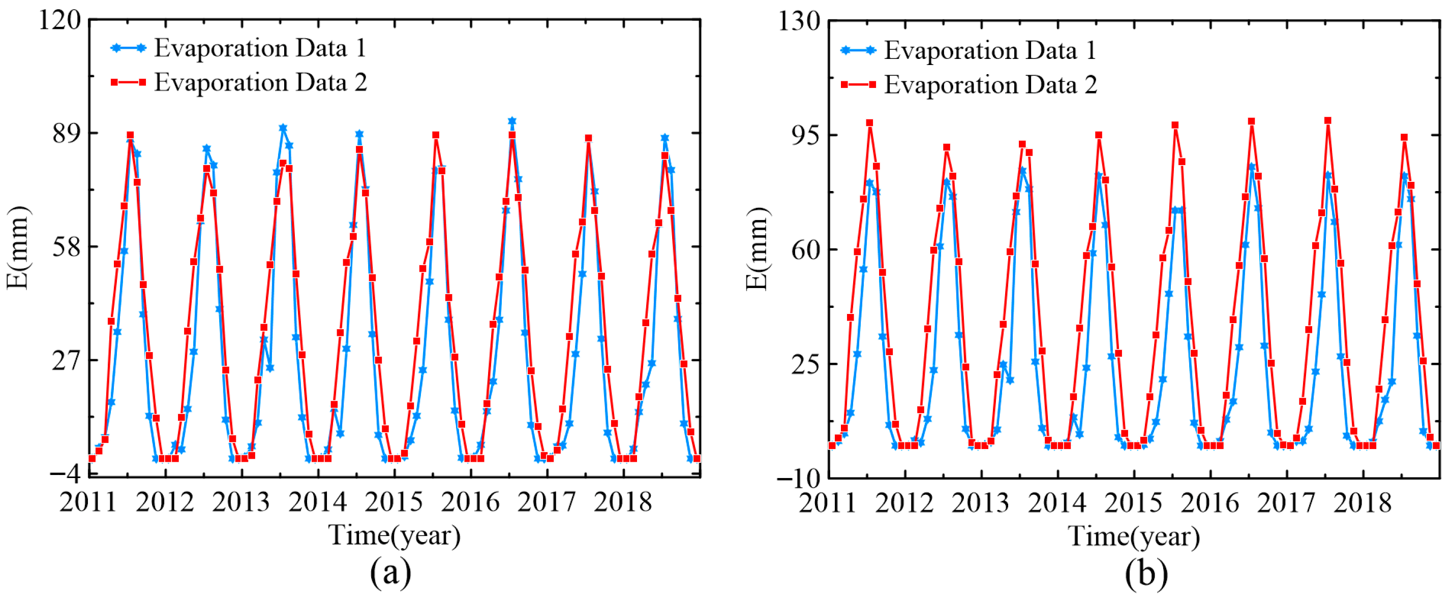
The ‘Evaporation dataset of the Tibetan Plateau at the monthly scale (1979–2018) V2.0’ (Evaporation Data 1) is a specialized evaporation model for the TP, which is supposed to be more reliable for our study area; however, it was terminated in 2018. The ‘1–km monthly potential evapotranspiration dataset for China (1901–2023)’ (Evaporation Data 2) and air temperature was used to supplement Evaporation Data 1 from 2019 to 2023, with three fitting methods, i.e., the proportional factor method, the polynomial function (after tests, the seventh-degree polynomial of the polynomial function was the best), and the exponential function (Table A1). Finally, the average values obtained from the three methods were used as the complemented evaporation data (Evaporation Data 1) from 2019 to 2023. Testing experiments were provided in Figure A1 and Figure A2 and Table A2, indicating the reliability of this processing.
Table A1. Fitting equations for complementing estimated lake/land evaporation results.
AreaFitting MethodsEquation
LakeProportional factor method E 1 l a k e i = a i × E 2 l a k e i
Seventh-degree polynomial E 1 l a k e = 2.624 × 10 7 × T 7 1.636 × 10 5 × T 6 3.17 × 10 4 × T 5 9.097 × 10 4 × T 4 + 0.035 × T 3 + 0.425 × T 2 + 3.826 × T + 27.26
Exponential function E 1 l a k e = 29.204 × e 0.122 × T
LandProportional factor method E 1 l a n d i = b i × E 2 l a n d i
Seventh-degree polynomial E 1 l a n d = 2.007 × 10 7 × T 7 1.308 × 10 5 × T 6 2.793 × 10 4 × T 5 1.418 × 10 3 × T 4 + 0.026 × T 3 + 0.463 × T 2 + 4.101 × T + 21.23
Exponential function E 1 l a n d = 24.167 × e 0.137 × T
Note: E 1 l a k e i / l a n d i is the lake/land evaporation to be estimated for the i th month in a year from 2019 to 2023, complementing Evaporation Data 1; E 2 l a k e i / l a n d i is the lake/land evaporation of E v a p o r a t i o n D a t a 2 for the i th month in a year from 2019 to 2023; a i / b i is the average ratio of Evaporation Data 1 to Evaporation Data 2 estimated with years from 2011 to 2018; T is the air temperature. Only the seventh-degree polynomials are shown here, because tests showed that they performed the best among polynomials of degree one to nine. E 1 l a k e / l a n d without subscript i for the seventh-degree polynomial and exponential function represents any monthly lake/land evaporation to be estimated from 2019 to 2023, which is estimated with the variable strongly correlated with evaporation, i.e., the air temperature T .
For the proportional factor method, the conversion coefficients derived from the correlation or similarity between Evaporation Data 1 and Evaporation Data 2 from 2011 to 2018 were used. We compared the lake evaporation and land evaporation of the two evaporation datasets, and the results showed high Pearson’s correlation coefficients both for lake surface (0.946) and land evaporation (0.938) (Figure A1). This provides feasibility for us to apply the proportional factor method to supplement Evaporation Data 1 based on Evaporation Data 2. However, for the seventh-degree polynomial and exponential function, the air temperature (T) from 2011 to 2018 was used for establishing the fitting functions.
Figure A1. Estimated evaporation with two evaporation datasets in Hala Lake basin from 2011 to 2018. (a) Lake surface evaporation; (b) land evaporation.
Remotesensing 17 03184 g0a1
Tests were also conducted to check the validity of the three fitting methods. We set tests using the data of 2011–2014, 2011–2015, and 2011–2016 in establishing the three fitting functions, and then calculated the evaporation in the remaining years. Meanwhile, we set the corresponding data of Evaporation Data 1 as the reference values for the calculation results. It was found that the calculated evaporation matched the reference well (Figure A2, Table A2), showing their rationality. Therefore, the average values obtained from the three methods were used as the final complemented evaporation data (Evaporation Data 1) from 2019 to 2023.
Figure A2. The estimated evaporation from different fitting methods and the reference. (a) Lake evaporation from 2011 to 2014 is used for establishing function fitting, and the estimated lake evaporation is from 2015 to 2018; (b) similar to (a) but for land evaporation; (c,d) estimated evaporation from 2016 to 2018; (e,f) estimated evaporation from 2017 to 2018.
Remotesensing 17 03184 g0a2
Table A2. Pearson’s correlation coefficients (rs) and RMSE between estimated evaporation and the reference shown in Figure A2.
StageAreas ConcernedProportional Factor Method (r/RMSE)Seven-Degree
Polynomial
(r/RMSE)
Exponential
Function (r/RMSE)
2015–2018Lake0.990/4.6110.989/4.5660.975/6.806
Land0.991/4.1100.991/3.9850.973/6.687
2016–2018Lake0.992/3.8640.990/4.4370.976/7.247
Land0.993/3.8560.992/3.6440.975/6.979
2017–2018Lake0.991/4.0710.993/4.0960.991/4.846
Land0.992/3.7810.993/3.4970.989/5.039

Appendix A.2. Pearson’s Correlation Coefficient (r)

r = ( X i X ¯ ) × ( Y i Y ¯ ) ( X i X ¯ ) 2 × ( Y i Y ¯ ) 2   ,
where   X i and Y i are the i th values for the two datasets, respectively, and X ¯ is the mean value of   X i , while Y ¯   is the mean value of   Y i .

Appendix A.3. Root Mean Square Error (RMSE) and Coefficient of Determination (R2)

R M S E = 1 n × i = 1 n ( y i y i ^   ) 2 ,
R 2 = 1 i = 1 n y i y i ^ 2 i = 1 n y i y ¯ 2   ,
where y i   is the values for the ith observation, y i ^   is the corresponding ith fitted or reference value, n is the number of observations in the sample, and y i ¯   is the mean value of y i .

Appendix A.4. Supplementing the Missing Monthly Lake Areas and Levels

Table A3. Stage fitting for filling the missing Hala Lake areas.
TimeFormulaR2RMSE
January 2011–August 2011 S = 1.368 × t 3 + 8268 × t 2 1.666 × 10 7 × t + 1.119 × 10 10 0.960920.36502
August 2011–August 2012 S = 16.03 × t 3 9.677 × 10 4 × t 2 + 1.947 × 10 8 × t 1.305 × 10 11 0.952130.52535
August 2012–May 2013 S = 12.74 × t 3 7.696 × 10 4 × t 2 + 1.549 × 10 8 × t 1.04 × 10 11 0.939760.37027
January 2013–December 2013 S = 15.007 × t 3 + 9.066 × t 2 1.826 × 10 8 × t + 1.225 × 10 11 0.841950.56017
October 2013–September 2014 S = 10.98 × t 3 6.633 × 10 4 × t 2 + 1.336 × 10 8 × t 8.968 × 10 10 0.939420.32695
April 2014–April 2015 S = 0.351 × t 3 + 2112.598 × t 2 4.235 × 10 6 × t + 2.829 × 10 9 0.808620.63627
April 2015–July 2016 S = 8.448 × t 3 5.11 × 10 4 × t 2 1.03 × 10 8 × t + 6.926 × 10 10 0.928480.76709
December 2015–November 2016 S = 11.767 × t 3 7.116 × 10 4 × t 2 + 1.434 × 10 8 × t 9.639 × 10 10 0.884780.829
November 2016–August 2017 S = 84.899 × t 3 5.138 × 10 5 × t 2 + 1.036 × 10 9 × t 6.968 × 10 11 0.943150.58407
May 2017–May 2018 S = 37.274 × t 3 2.257 × 10 5 × t 2 + 4.554 × 10 8 × t 3.063 × 10 11 0.900910.8469
May 2018–February 2019 S = 34.833 × t 3 2.11 × 10 5 × t 2 + 4.26 × 10 8 × t 2.867 × 10 11 0.976530.85701
February 2019–April 2020 S = 9.061 × t 3 + 5.492 × 10 4 × t 2 1.109 × 10 8 × t + 7.471 × 10 10 0.978340.87676
April 2020–January 2021 S = 20.517 × t 3 + 1.244 × 10 5 × t 2 2.513 × 10 8 × t + 1.692 × 10 11 0.966990.24712
January 2021–June 2022 S = 4.929 × t 3 + 2.989 × 10 4 × t 2 6.041 × 10 7 × t + 4.07 × 10 10 0.993040.18264
June 2022–January 2023 S = 105.711 × t 3 6.415 × 10 5 × t 2 + 1.298 × 10 9 × t 8.751 × 10 11 0.951840.57042
January 2023–December 2023 S = 21.92 × t 3 + 1.331 × 10 5 × t 2 2.692 × 10 8 × t + 1.816 × 10 11 0.96690.34917
t is time (year); S is the lake area (km2).
Table A4. Similar to Table A3, but for filling the missing Hala Lake levels.
Satellite MissionTimeFormulaR2RMSE
CryoSat–2January 2011–January 2012 H = 2.066 × t 3 + 1.247 × 10 4 × t 2 2.508 × 10 7 × t + 1.681 × 10 10 0.770330.06981
February 2012–January 2013 H = 1.831 × t 3 + 1.105 × 10 4 × t 2 2.225 × 10 7 × t + 1.492 × 10 10 0.419250.10762
January 2013–September 2013 H = 1.604 × t 3 9.689 × 10 3 × t 2 + 1.951 × 10 7 × t 1.31 × 10 10 0.831360.02836
September 2013–February 2014 H = 22.722 × t 3 + 1.373 × 10 5 × t 2 2.765 × 10 8 × t + 1.826 × 10 11 0.163470.13088
February 2014–July 2014 H = 71.37 × t 3 4.313 × 10 5 × t 2 + 8.387 × 10 8 × t 5.833 × 10 11 0.975930.03783
July 2014–April 2015 H = 6.258 × t 3 + 3.783 × 10 4 × t 2 7.623 × 10 7 × t + 5.121 × 10 10 0.881330.06762
May 2015–December 2015 H = 15.865 × t 3 9.594 × 10 4 × t 2 + 1.934 × 10 8 × t 1.299 × 10 11 0.865180.08123
December 2015–August 2016 H = 9.852 × t 3 5.959 × 10 4 × t 2 + 1.202 × 10 8 × t 8.075 × 10 10 0.527870.09532
August 2016–March 2017 H = 3.785 × t 3 2.29 × 10 4 × t 2 + 4.618 × 10 7 × t 3.104 × 10 10 0. 973720.01561
March 2017–August 2017 H = 17.555 × t 3 + 1.063 × 10 5 × t 2 2.144 × 10 8 × t + 1.442 × 10 11 0.842560.10563
August 2017–February 2018 H = 12.452 × t 3 7.537 × 10 4 × t 2 + 1.521 × 10 8 × t 1.023 × 10 11 0.61950.06853
April 2018–November 2018 H = 26.677 × t 3 + 1.615 × 10 5 × t 2 3.261 × 10 8 × t + 2.194 × 10 11 0.895390.08445
November 2018–July 2019 H = 6.045 × t 3 3.662 × 10 4 × t 2 + 7.393 × 10 7 × t 4.976 × 10 10 0.954370.05678
July 2019–November 2019 H = 82.468 × t 3 + 4.997 × 10 5 × t 2 1.009 × 10 9 × t + 6.794 × 10 11 0.999990.00043
November 2019–May 2020 H = 6.708 × t 3 4.065 × 10 4 × t 2 + 8.213 × 10 7 × t 5.531 × 10 10 0.874890.08814
May 2020–December 2020 H = 15.218 × t 3 + 9.2254 × 10 4 × t 2 1.864 × 10 8 × t + 1.256 × 10 11 0.917560.03545
December 2020–July 2021 H = 17.66 × t 3 + 1.071 × 10 5 × t 2 2.164 × 10 8 × t + 1.458 × 10 11 0.999990.00005
July 2021–March 2022 H = 10.829 × t 3 + 6.568 × 10 4 × t 2 1.328 × 10 8 × t + 8.951 × 10 10 0.885670.05877
October 2021–September 2022 H = 1.573 × t 3 9.543 × 10 3 × t 2 + 1.93 × 10 7 × t 1.301 × 10 10 0.951460.04179
October 2022–September 2023 H = 0.925 × t 3 + 5.614 × 10 3 × t 2 1.136 × 10 7 × t + 7.665 × 10 9 0.962480.02657
May 2023–December 2023 H = 3.722 × t 3 2.26 × 10 5 × t 2 + 4.572 × 10 7 × t 3.084 × 10 10 0.999990.00001
ICESat–2October 2018–March 2019 H = 41.585 × t 3 + 2.519 × 10 5 × t 2 5.086 × 10 8 × t + 3.423 × 10 11 0.999960.0003
December 2018–September 2019 H = 0.854 × t 3 5.174 × 10 3 × t 2 + 1.045 × 10 7 × t 7.03 × 10 9 0.978980.04487
September 2019–September 2020 H = 1.416 × t 3 + 8.581 × 10 3 × t 2 1.734 × 10 7 × t + 1.168 × 10 10 0.990890.00791
September 2020–July 2021 H = 0.666 × t 3 4.035 × 10 3 × t 2 + 8.153 × 10 6 × t 5.491 × 10 9 0.876720.02995
July 2021–April 2022 H = 5.021 × t 3 3.045 × 10 4 × t 2 + 6.157 × 10 7 × t 4.15 × 10 10 0.848270.0398
December 2021–July 2022 H = 3.604 × t 3 2.186 × 10 4 × t 2 + 4.422 × 10 7 × t 2.981 × 10 10 0.518130.04604
June 2022–January 2023 H = 11.289 × t 3 6.851 × 10 4 × t 2 + 1.386 × 10 8 × t 9.344 × 10 10 0.88780.03431
January 2023–December 2023 H = 3.211 × t 3 + 1.949 × 10 4 × t 2 3.944 × 10 8 × t + 2.66 × 10 10 0.821090.04359
t is time (year); H is the water level (m).
Table A5. Lake level–area relationship for filling the missing Hala Lake areas.
ModelNameFormulaR2RMSE
Polynomial functionsFirst-degree polynomial S = 11.876 × H 4.783 × 10 4 0.985681.65424
Second-degree polynomial S = 0.406 × H 2 3.3 × 10 3 × H + 6.709 × 10 6 0.986141.62744
Third-degree polynomial S = 0.78 × H 3 + 9.55 × 10 3 × H 2 3.897 × 10 7 × H + 5.301 × 10 10 0.987031.57446
Fourth-degree polynomial S = 0.637 × H 4 + 1.04 × 10 4 × H 3 6.362 × 10 7 × H 2 + 1.731 × 10 11 × H 1.765 × 10 14 0.987641.53703
Fifth-degree polynomial S = 1.428 × 10 4 × H 5 + 1.739 × H 4 4.605 × 10 3 × H 3 2.031 × 10 7 × H 2 + 1.212 × 10 11 × H 1.64 × 10 14 0.988141.50537
Sixth-degree polynomial S = 4.686 × 10 8 × H 6 + 7.008 × 10 4 × H 5 3.766 × H 4 + 8.452 × 10 3 × H 3 8.521 × 10 6 × H 2 + 1.741 × 10 10 × H 3.585 × 10 13 0.988121.50655
Seventh-degree polynomial S = 1.357 × 10 11 × H 7 1.653 × 10 7 × H 6 1.741 × 10 5 × H 5 + 8.184 × H 4 3.781 × 10 4 × H 3 + 2.19 × 10 7 × H 2 + 1.931 × 10 11 × H 3.257 × 10 14 0.988401.48846
Eighth-degree polynomial S = 2.838 × 10 14 × H 8 + 3.641 × 10 10 × H 7 8.919 × 10 7 × H 6 5.872 × 10 3 × H 5 + 26.389 × H 4 + 2.38 × 10 4 × H 3 2.109 × 10 8 × H 2 + 6.543 × 10 10 × H 3.947 × 10 14 0.978052.04792
Ninth-degree polynomial S = 0.14 × 10 17 × H 9 2.388 × 10 14 × H 8 + 5.218 × 10 10 × H 7 2.408 × 10 6 × H 6 + 1.158 × 10 3 × H 5 0.672 × H 4 + 8.447 × 10 4 × H 3 9.657 × 10 7 × H 2 7.988 × 10 11 × H + 1.569 × 10 15 0.983551.77295
Exponential functionsSingle exponential model S = 1.095 × 10 31 × e 0.019 × H 0.98591.6576
Binomial exponential model S = 0 * × e 1.566 × H + 1.095 × 10 31 × e 0.19 × H 0.98591.6741
Power functionsSingle power model S = 1.418 × 10 278 × H 77.73 0.985891.6577
Binomial power model S = 1.417 × 10 278 × H 77.73 + 0 * 0.985891.6659
H is the water level (m); S is the lake area (km2); 0* represents a very small numerical value.
Table A6. Similar to Table A5, but for filling the missing Hala Lake levels.
ModelNameFormulaR2RMSE
Polynomial functionsFirst-degree polynomial H = 0.087 × S + 4026.534 0.979110.17436
Second-degree polynomial H = 3.917 × 10 4 × S 2 + 0.575 × S + 3874.167 0.980340.16917
Third-degree polynomial H = 1.156 × 10 5 × S 3 + 0.021 × S 2 12.86 × S + 6660 .4420.980430.16878
Fourth-degree polynomial H = 3.975 × 10 6 × S 4 9.911 × 10 3 × S 3 + 9.266 × S 2 3849.357 × S + 6.036 × 10 5 0.981460.16429
Fifth-degree polynomial H = 3.204 × 10 7 × S 5 + 1.002 × 10 3 × S 4 1.252 × S 3 + 782.708 × S 2 2.446 × 10 5 × S + 3.057 × 10 7 0.982170.1611
Sixth-degree polynomial H = 5.877 × 10 8 × S 6 + 2.193 × 10 4 × S 5 0.341 × S 4 + 282.456 × S 3 1.317 × 10 5 × S 2 + 3.273 × 10 7 × S 3.39 × 10 9 0.983640.15433
Seventh-degree polynomial H = 1.74 × 10 9 × S 7 7.639 × 10 6 × S 6 + 0.014 × S 5 15.024 × S 4 + 9420.678 × S 3 3.544 × 10 6 × S 2 + 7.404 × 10 8 × S 6.63 × 10 10 0.983750.15380
Eighth-degree polynomial H = 8.942 × 10 11 × S 8 4.439 × 10 7 × S 7 + 9.642 × 10 4 × S 6 1.196 × S 5 + 927.67 × S 4 4.603 × 10 5 × S 3 + 1.427 × 10 8 × S 2 2.529 × 10 10 × S + 1.96 × 10 12 0.98370.15404
Ninth-degree polynomial H = 7.022 × 10 14 × S 9 + 4.425 × 10 10 × S 8 1.223 × 10 6 × S 7 + 1.949 × 10 3 × S 6 1.979 × S 5 + 1329.731 × S 4 5.918 × 10 5 × S 3 + 1.684 × 10 8 × S 2 2.781 × 10 10 × S + 2.032 × 10 12 0.9840.15259
Exponential functionsSingle exponential model H = 4027 × e 2.12 × 10 5 × S 0.979110.17552
Binomial exponential model H = 4027 × e 2.12 × 10 5 × S + 0 * × e 0.108 × S 0.979110.17667
Power functionsSingle power model H = 3748 × S 0.013 0.97950.17384
Binomial power model H = 3.452 × 10 13 × S 4.457 + 4093 0.980310.17094
H is the water level (m). S is the lake area (km2). 0* represents a very small numerical value.

Appendix A.5. Exhibition of Glacier Melting Cases
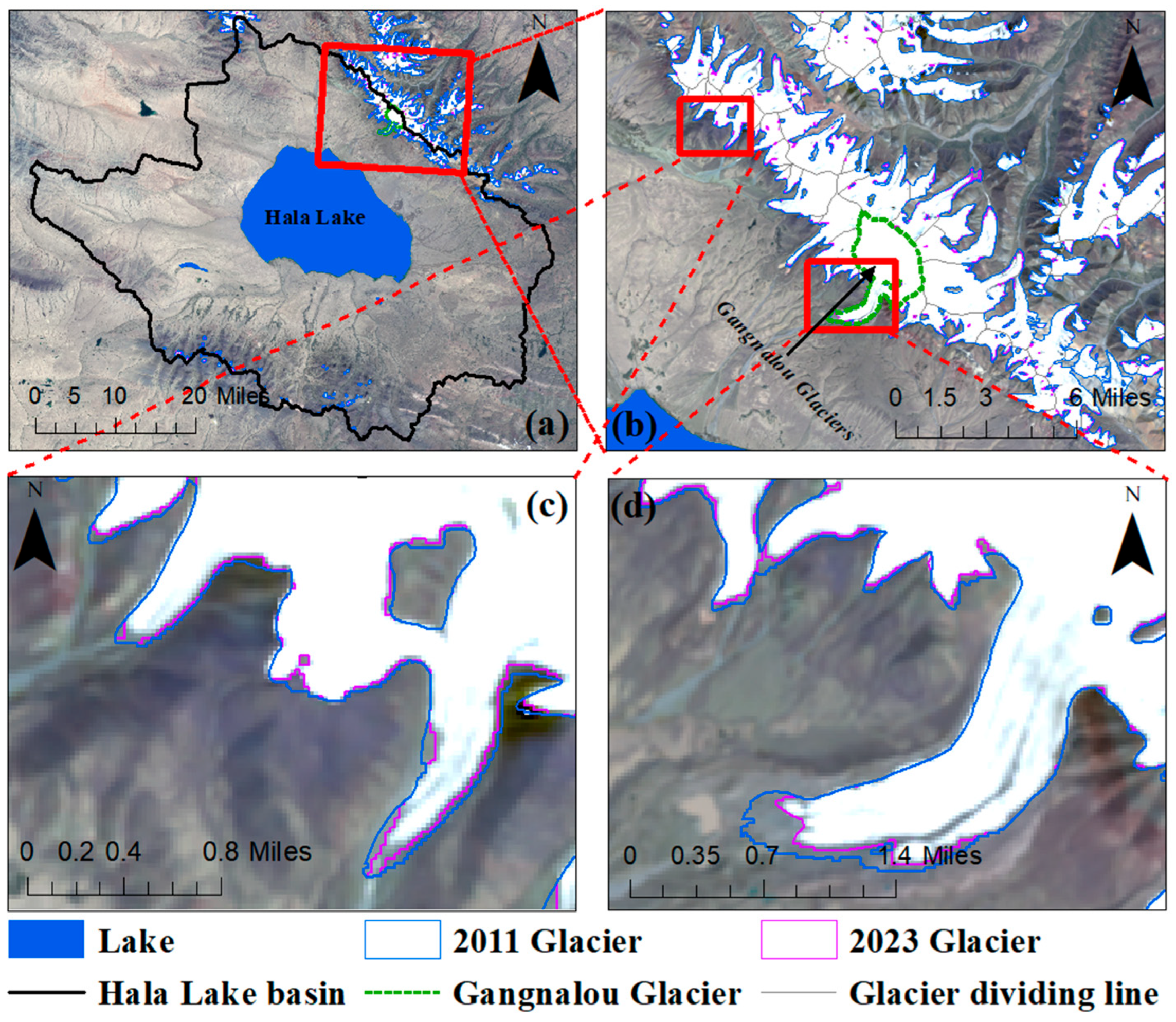
Figure A3. The evident retreat of Gangnalou glacier and its surrounding glaciers from 2011 to 2023. (a) Location of the Gangnalou glacier and its surrounding glaciers w.r.t. Hala Lake, (b) close view of the glacier, (c,d) detailed views on selected areas with glacial retreat.
Remotesensing 17 03184 g0a3

References

  1. Zhao, S. A new scheme for comprehensive physical regionalization in China. Acta Geogr. Sin. 1983, 38, 1–10. [Google Scholar]
  2. Liu, X.; Chen, B. Climatic warming in the Tibetan Plateau during recent decades. Int. J. Climatol. 2000, 20, 1729–1742. [Google Scholar] [CrossRef]
  3. Zhang, G.; Luo, W.; Chen, W.; Zheng, G. A robust but variable lake expansion on the Tibetan Plateau. Sci. Bull. 2019, 64, 1306–1309. [Google Scholar] [CrossRef]
  4. Zhang, G.; Yao, T.; Chen, W.; Zheng, G.; Shum, C.K.; Yang, K.; Piao, S.; Sheng, Y.; Yi, S.; Li, J.; et al. Regional differences of lake evolution across China during 1960s–2015 and its natural and anthropogenic causes. Remote Sens. Environ. 2019, 221, 386–404. [Google Scholar] [CrossRef]
  5. Jin, Z.; You, Q.; Wu, F.; Sun, B.; Cai, Z. Changes of climate and climate extremes in the three-rivers headwaters’ region over the Tibetan plateau during the past 60 years. Trans. Atmos. Sci. 2020, 43, 1042–1055. [Google Scholar]
  6. Zhu, L.; Zhang, G.; Yang, R.; Liu, C.; Yang, K.; Qiao, B.; Han, B. Lake variations on Tibetan Plateau of recent 40 years and future changing tendency. Bull. Chin. Acad. Sci. 2019, 34, 1254–1263. [Google Scholar] [CrossRef]
  7. Yao, T. Glacial fluctuations and its impacts on lakes in the southern Tibetan Plateau. Chin. Sci. Bull. 2010, 55, 2071. [Google Scholar] [CrossRef]
  8. Zhang, G.; Chen, W.; Xie, H. Tibetan Plateau’s Lake Level and Volume Changes from NASA’s ICESat/ICESat-2 and Landsat Missions. Geophys. Res. Lett. 2019, 46, 13107–13118. [Google Scholar] [CrossRef]
  9. Yang, R.; Zhu, L.; Wang, J.; Ju, J.; Ma, Q.; Turner, F.; Guo, Y. Spatiotemporal variations in volume of closed lakes on the Tibetan Plateau and their climatic responses from 1976 to 2013. Clim. Chang. 2017, 140, 621–633. [Google Scholar] [CrossRef]
  10. Zhang, J.; Hu, Q.; Li, Y.; Li, H.; Li, J. Area, lake-level and volume variations of typical lakes on the Tibetan Plateau and their response to climate change, 1972–2019. Geo-Spat. Inf. Sci. 2021, 24, 458–473. [Google Scholar] [CrossRef]
  11. Sun, K.; Chen, J.; Lhakpa, D.; He, H.; Duan, Z. Estimating the lake storage capacity on the Tibetan Plateau using satellite altimetry and imagery data: A comparative analysis of water volume change methods. J. Mt. Sci. 2025, 22, 1388–1404. [Google Scholar] [CrossRef]
  12. Luo, S.; Song, C.; Zhan, P.; Liu, K.; Chen, T.; Li, W.; Ke, L. Refined estimation of lake water level and storage changes on the Tibetan Plateau from ICESat/ICESat-2. Catena 2021, 200, 105177. [Google Scholar] [CrossRef]
  13. Chen, J.; Gao, J.; Wang, Y.; Jin, L. Estimation of Water Volume Changes in Typical Alpine Lakes on the Tibetan Plateau by Combining Sentinel-3 Radar Altimetry Data and Optical Images. Mt. Res. 2023, 41, 926–940. [Google Scholar]
  14. Zheng, J.; Ke, C.; Shao, Z.; Lie, F. Monitoring changes in the water volume of Hulun Lake by integrating satellite altimetry data and Landsat images between 1992 and 2010. J. Appl. Remote Sens. 2016, 10, 016029. [Google Scholar] [CrossRef]
  15. Yang, X.; Wang, N.; Chen, A.; He, J.; Hua, T.; Qie, Y. Changes in area and water volume of the Aral Sea in the arid Central Asia over the period of 1960–2018 and their causes. Catena 2020, 191, 104566. [Google Scholar] [CrossRef]
  16. Lu, Y.; Wu, A. Natural situation and vegetation types of Lake Hala in Qinghai province. Grassl. China 1984, 2, 27–31. [Google Scholar]
  17. Li, D.; Cui, B.; Wang, Y.; Xiao, B.; Jiang, B. Glacier extent changes and possible causes in the Hala Lake Basin of Qinghai–Tibet Plateau. J. Mt. Sci. 2019, 16, 1571–1583. [Google Scholar] [CrossRef]
  18. Wang, R.; Zhang, Y.; Wuennemann, B.; Biskaborn, B.K.; Yin, H.; Xia, F.; Zhou, L.; Diekmann, B. Linkages between Quaternary climate change and sedimentary processes in Hala Lake, northern Tibetan Plateau, China. J. Asian Earth Sci. 2015, 107, 140–150. [Google Scholar] [CrossRef]
  19. Cao, J.; Zhang, J.; Zhang, C.; Chen, F. Environmental changes during the past 800 years recorded in lake sediments from Hala Lake on the Northern Tibetan Plateau. Quat. Sci. 2007, 27, 100–107. [Google Scholar]
  20. Yan, D.; Wuennemann, B. Late Quaternary water depth changes in Hala Lake, northeastern Tibetan Plateau, derived from ostracod assemblages and sediment properties in multiple sediment records. Quat. Sci. Rev. 2014, 95, 95–114. [Google Scholar] [CrossRef]
  21. He, M.; Fang, H.; Zhu, Y.; Sun, Z.; Hu, X.; Zhang, P.; Wang, X.; Pei, F.; Qiu, G.; Du, B.; et al. A study of geological structural features of Hala Lake Depression in Qilian Mountain and reservoir-forming conditions of natural gas hydrate. Geol. China 2020, 47, 173–187. [Google Scholar]
  22. Li, D.; Zhang, R.; Cui, B.; Zhao, Y.; Wang, Y.; Jiang, B. Response of lake dynamics to climate change in the Hala Lake basin of Tibetan Plateau from 1986 to 2015. J. Nat. Resour. 2021, 36, 501–512. [Google Scholar] [CrossRef]
  23. Wang, R.; Liu, B.; Huang, B. Analysis of Dynamic Change and Causes of the Area of Hala Lake from 1986 to 2019. Pearl River. 2021, 42, 20–25+33. [Google Scholar]
  24. Wu, H.; Yang, M.; Yang, C.; Li, Y. Effect of glacier mass loss on water level fluctuation of lake in Hala Lake basin. J. Water Resour. Water Eng. 2016, 27, 13–20. [Google Scholar]
  25. Jiang, Z.; Wang, J.; Cai, X.; Zhao, J.; Zhang, H.; Zhang, Y.; Wang, C. Hydrological Characteristics Change of Hala Lake and Its Response to Climate Change, 1987–2018. Remote Sens. 2022, 14, 2886. [Google Scholar] [CrossRef]
  26. Guo, L.; Li, J.; Charrier, L.; Dehecq, A.; Beraud, L.; Li, Z.; Li, X.; Zhu, J.; Li, L.; Wang, Y. Surging Processes and Mechanisms at Small Glaciers in the Qilian Mountains, Northwestern China, Revealed by Long-Term, Temporally Dense Remote Sensing Observations. J. Geophys. Res. Earth Surf. 2025, 130, e2024JF008157. [Google Scholar] [CrossRef]
  27. Jiang, L.; Nielsen, K.; Andersen, O.B.; Bauer-Gottwein, P. Monitoring recent lake level variations on the Tibetan Plateau using CryoSat-2 SARIn mode data. J. Hydrol. 2017, 544, 109–124. [Google Scholar] [CrossRef]
  28. Labroue, S.; Boy, F.; Picot, N.; Urvoy, M.; Ablain, M. First quality assessment of the Cryosat-2 altimetric system over ocean. Adv. Space Res. 2012, 50, 1030–1045. [Google Scholar] [CrossRef]
  29. Siegfried, M.R.; Fricker, H.A.; Roberts, M.; Scambos, T.A.; Tulaczyk, S. A decade of West Antarctic subglacial lake interactions from combined ICESat and CryoSat-2altimetry. Geophys. Res. Lett. 2014, 41, 891–898. [Google Scholar] [CrossRef]
  30. Wei, X.; Li, F.; Zhang, S.; Hao, W. CryoSat-2 satellite altimetry and its application. Chin. J. Polar Res. 2015, 27, 446–453. [Google Scholar]
  31. Donlon, C.; Berruti, B.; Buongiorno, A.; Ferreira, M.H.; Femenias, P.; Frerick, J.; Goryl, P.; Klein, U.; Laur, H.; Mavrocordatos, C.; et al. The Global Monitoring for Environment and Security (GMES) Sentinel-3 mission. Remote Sens. Environ. 2012, 120, 37–57. [Google Scholar] [CrossRef]
  32. Jiang, L.; Nielsen, K.; Dinardo, S.; Andersen, O.B.; Bauer-Gottwein, P. Evaluation of Sentinel-3 SRAL SAR altimetry over Chinese rivers. Remote Sens. Environ. 2020, 237, 111546. [Google Scholar] [CrossRef]
  33. Parrish, C.E.; Magruder, L.A.; Neuenschwander, A.L.; Forfinski-Sarkozi, N.; Alonzo, M.; Jasinski, M. Validation of ICESat-2 ATLAS Bathymetry and Analysis of ATLAS’s Bathymetric Mapping Performance. Remote Sens. 2019, 11, 1634. [Google Scholar] [CrossRef]
  34. Xu, F.; Zhang, G.; Yi, S.; Chen, W. Seasonal trends and cycles of lake–level variations over the Tibetan Plateau using multi-sensor altimetry data. J. Hydrol. 2022, 604, 127251. [Google Scholar] [CrossRef]
  35. Markus, T.; Neumann, T.; Martino, A.; Abdalati, W.; Brunt, K.; Csatho, B.; Farrell, S.; Fricker, H.; Gardner, A.; Harding, D.; et al. The Ice, Cloud, and land Elevation Satellite-2 (ICESat-2): Science requirements, concept, and implementation. Remote Sens. Environ. 2017, 190, 260–273. [Google Scholar] [CrossRef]
  36. Cretaux, J.F.; Abarca-del-Rio, R.; Berge-Nguyen, M.; Arsen, A.; Drolon, V.; Clos, G.; Maisongrande, P. Lake Volume Monitoring from Space. Surv. Geophys. 2016, 37, 269–305. [Google Scholar] [CrossRef]
  37. Peng, S.; Ding, Y.; Liu, W.; Li, Z. 1 km monthly temperature and precipitation dataset for China from 1901 to 2017. Earth Syst. Sci. Data 2019, 11, 1931–1946. [Google Scholar] [CrossRef]
  38. Wang, L.; Han, S.; Tian, F.; Li, K.; Li, Y.; Tudaji, M.; Cao, X.; Nan, Y.; Cui, T.; Zheng, X.; et al. The Evaporation on the Tibetan Plateau Stops Increasing in the Recent Two Decades. J. Geophys. Res.-Atmos. 2022, 127, e2022JD037377. [Google Scholar] [CrossRef]
  39. Ding, Y.; Peng, S. Spatiotemporal change and attribution of potential evapotranspiration over China from 1901 to 2100. Theor. Appl. Climatol. 2021, 145, 79–94. [Google Scholar] [CrossRef]
  40. Rodell, M.; Houser, P.; Jambor, U.; Gottschalck, J.; Mitchell, K.; Meng, C.-J.; Arsenault, K.; Cosgrove, B.; Radakovich, J.; Bosilovich, M.; et al. The global land data assimilation system. Bull. Am. Meteorol. Soc. 2004, 85, 381–394. [Google Scholar] [CrossRef]
  41. Du, Z.; Li, W.; Zhou, D.; Tian, L.; Ling, F.; Wang, H.; Gui, Y.; Sun, B. Analysis of Landsat-8 OLI imagery for land surface water mapping. Remote Sens. Lett. 2014, 5, 672–681. [Google Scholar] [CrossRef]
  42. Wang, X.; Xie, S.; Du, J. Water index formulation and its effectiveness research on the complicated surface water surroundings. Natl. Remote Sens. Bull. 2018, 22, 360–372. [Google Scholar] [CrossRef]
  43. McFeeters, S.K. The use of the normalized difference water index (NDWI) in the delineation of open water features. Int. J. Remote Sens. 1996, 17, 1425–1432. [Google Scholar] [CrossRef]
  44. Ma, W.; Bai, L.; Ma, W.; Hu, W.; Xie, Z.; Su, R.; Wang, B.; Ma, Y. Interannual and Monthly Variability of Typical Inland Lakes on the Tibetan Plateau Located in Three Different Climatic Zones. Remote Sens. 2022, 14, 5015. [Google Scholar] [CrossRef]
  45. Wang, Y.; Li, J.; Guo, M.; Bao, A.; Hu, R.; Zhao, S. Time-series analysis of Sayram Lake area changes during 1989–2014. Arid Land Geogr. 2016, 39, 851–860. [Google Scholar]
  46. Munyaneza, O.; Wali, U.G.; Uhlenbrook, S.; Maskey, S.; Mlotha, M.J. Water level monitoring using radar remote sensing data: Application to Lake Kivu, central Africa. Phys. Chem. Earth 2009, 34, 722–728. [Google Scholar] [CrossRef]
  47. Cai, X.; Gan, W.; Ji, W.; Zhao, X.; Wang, X.; Chen, X. Optimizing Remote Sensing-Based Level–Area Modeling of Large Lake Wetlands: Case Study of Poyang Lake. IEEE J. Sel. Top. Appl. Earth Obs. Remote Sens. 2015, 8, 471–479. [Google Scholar] [CrossRef]
  48. Ling, F.; Cai, X.; Li, W.; Xiao, F.; Li, X.; Du, Y. Monitoring river discharge with remotely sensed imagery using river island area as an indicator. J. Appl. Remote Sens. 2012, 6, 063564. [Google Scholar] [CrossRef]
  49. Zhu, W.; Jia, S.; Lv, A. Monitoring the Fluctuation of Lake Qinghai Using Multi–Source Remote Sensing Data. Remote Sens. 2014, 6, 10457–10482. [Google Scholar] [CrossRef]
  50. Chen, P.; An, Z.; Xue, H.; Yao, Y.; Yang, X.; Wang, R.; Wang, Z. INPPTR: An improved retracking algorithm for inland water levels estimation using Cryosat-2 SARin data. J. Hydrol. 2022, 613, 128439. [Google Scholar] [CrossRef]
  51. Hartigan, J.A.; Wong, M.A. Algorithm AS 136: A k-means clustering algorithm. Appl. Stat. 1979, 28, 100–108. [Google Scholar] [CrossRef]
  52. Li, J.; Hua, C.; Yang, Y.; Guan, X. Bayesian Block Structure Sparse Based T–S Fuzzy Modeling for Dynamic Prediction of Hot Metal Silicon Content in the Blast Furnace. IEEE Trans. Ind. Electron. 2018, 65, 4933–4942. [Google Scholar] [CrossRef]
  53. Yuan, C.; Gong, P.; Bai, Y. Performance Assessment of ICESat-2 Laser Altimeter Data for Water–Level Measurement over Lakes and Reservoirs in China. Remote Sens. 2020, 12, 770. [Google Scholar] [CrossRef]
  54. Chen, J.; Liu, Y.; Cao, L.; Hu, J.; Liu, S. A review on the research of remote sensing monitoring of lake changes and quantitative estimation of lake water balance in Qinghai–Tibet Plateau. J. Glaciol. Geocryol. 2022, 44, 1203–1215. [Google Scholar]
  55. Taube, C.M. Three methods for computing the volume of a lake. In Manual of Fisheries Survey Methods II: With Periodic Updates; Schneider, J.C., Ed.; Michigan Department of Natural Resources: Ann Arbor, MI, USA, 2000; Volume 25, pp. 175–179. [Google Scholar]
  56. Qiao, B.; Zhu, L. Differences and cause analysis of changes in lakes of different supply types in the north-western Tibetan Plateau. Hydrol. Process. 2017, 31, 2752–2763. [Google Scholar] [CrossRef]
  57. Hall, D.K.; Riggs, G.A.; Salomonson, V.V. Development of methods for mapping global snow cover using moderate resolution imaging spectroradiometer data. Remote Sens. Environ. 1995, 54, 127–140. [Google Scholar] [CrossRef]
  58. Liu, S.; Sun, W.; Shen, Y.; Li, G. Glacier changes since the Little Ice Age maximum in the western Qilian Shan, northwest China, and consequences of glacier runoff for water supply. J. Glaciol. 2003, 49, 117–124. [Google Scholar] [CrossRef]
  59. Adler, J.; Parmryd, I. Quantifying Colocalization by Correlation: The Pearson Correlation Coefficient is Superior to the Mander’s Overlap Coefficient. Cytom. Part A 2010, 77, 733–742. [Google Scholar] [CrossRef] [PubMed]
  60. Liu, S.; Yao, X.; Guo, W.; Xu, J.; Shangguan, D.; Wei, J.; Bao, W.; Wu, L. The contemporary glaciers in China based on the Second Chinese Glacier Inventory. Acta Geogr. Sin. 2015, 70, 3–16. [Google Scholar]
  61. Bianduo; Bianbaciren; Li, L.; Wang, W.; Zhaxiyangzong. The response of lake change to climate fluctuation in north Qinghai–Tibet Plateau in last 30 years. J. Geog. Sci. 2009, 19, 131–142. [Google Scholar] [CrossRef]
  62. Lei, Y.; Yang, K. The cause of rapid lake expansion in the Tibetan Plateau: Climate wetting or warming? WIREs Water 2017, 4, e1236. [Google Scholar] [CrossRef]
  63. Mao, D.; Wang, Z.; Yang, H.; Li, H.; Thompson, J.R.; Li, L.; Song, K.; Chen, B.; Gao, H.; Wu, J. Impacts of Climate Change on Tibetan Lakes: Patterns and Processes. Remote Sens. 2018, 10, 358. [Google Scholar] [CrossRef]
  64. Chen, R.; Duan, K.; Shang, W.; Shi, P.; Meng, Y.; Zhang, Z. Increase in seasonal precipitation over the Tibetan Plateau in the 21st century projected using CMIP6 models. Atmos. Res. 2022, 277, 106306. [Google Scholar] [CrossRef]
  65. Qiu, H.; Zhou, T.; Zou, L.; Jiang, J.; Chen, X.; Hu, S. Future changes in precipitation and water availability over the Tibetan Plateau projected by CMIP6 models constrained by climate sensitivity. Atmos. Ocean. Sci. Lett. 2024, 17, 100537. [Google Scholar] [CrossRef]
  66. Wang, K.; Song, X.; Lu, F.; Yu, S.; Zhou, Y.; Sun, J. CMIP6 Simulation-Based Daily Surface Air Temperature and Precipitation Projections over the Qinghai-Tibetan Plateau in the 21st Century. Atmosphere 2024, 15, 434. [Google Scholar] [CrossRef]
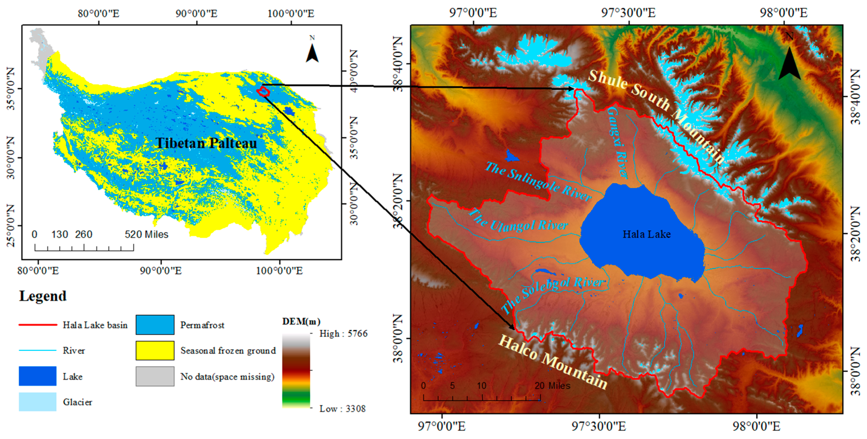
Figure 1. Geographic overview of the Hala Lake basin.
Remotesensing 17 03184 g001
Figure 2. The supplemented complete time series of monthly (a) lake area and (b) lake level changes, and (c) the derived LWSC time series for the period 2011–2023. The lake area and lake level changes were retrieved using the Stage Fitting (SF) method and the Level–Area relationship (LA) method. The LWSC was derived from lake area and lake level changes. The bar chart shows the monthly LWSC.
Remotesensing 17 03184 g002
Figure 3. (a) Correlations between seasonal monitored LWSC (dark blue line) and two climate factors: net precipitation (light blue bars) and air temperature changes (red line). (b) Correlation between yearly monitored LWSC (blue line with dots) and yearly net precipitation (purple line with stars).
Remotesensing 17 03184 g003
Figure 4. Estimated glacier area, meltwater changes, and summer air temperature in the Hala Lake basin (2011–2023).
Remotesensing 17 03184 g004
Figure 5. Comparison between the estimated and the monitored LWSC.
Remotesensing 17 03184 g005
Figure 6. The strong correlations between the Hala Lake areas (a) and water levels (b) in this study and those from Hydroweb.
Remotesensing 17 03184 g006
Figure 7. Comparison between glacier area results in this study and those from Jiang et al. (2022) [25]. The inset shows strong correlation between the two glacier area datasets.
Remotesensing 17 03184 g007
Table 1. Information on image data used in this study.
MissionSensorLaunch TimeRepetition
Period (Day)
Spatial
Resolution(m)
Number of Images (Scene)
Landsat 5TMAugust 198416303
Landsat 7ETM+April 1999163031
Landsat 8OLI/TIRSFebruary 2013163058
Landsat 9OLI–2/TIRS–2September 2021163013
Table 2. Mean yearly contributions of water balance components at the three different stages and the entire study period.
Water Balance
Components
Mean Yearly Contributions (km3)
201120142015–20192020–20232011–2023
Recharge P L 0.173   ± 0.026 0.194   ± 0.028 0.159   ± 0.020 0.177   ± 0.01551.00%
R P 0.177   ± 0.218 0.256   ± 0.210 0.036   ± 0.131 0.142   ± 0.11240.96%
G 0.021   ± 0.015 0.038   ± 0.035 0.022   ± 0.018 0.028   ± 0.0158.04%
Water loss E L 0.206   ± 0.011 0.199   ± 0.013 0.215   ± 0.014 0.206   ± 0.00759.37%
Disclaimer/Publisher’s Note: The statements, opinions and data contained in all publications are solely those of the individual author(s) and contributor(s) and not of MDPI and/or the editor(s). MDPI and/or the editor(s) disclaim responsibility for any injury to people or property resulting from any ideas, methods, instructions or products referred to in the content.