Article

A Spectral Mode Reconstruction Method for Floating Target Detection Under Strong Sea Clutter Conditions

1
Information Fusion Institute, Naval Aviation University, Yantai 264001, China
2
Yantai Research Institute, Harbin Engineering University, Yantai 265500, China
*
Author to whom correspondence should be addressed.
Remote Sens. 2025, 17(18), 3155; https://doi.org/10.3390/rs17183155
Submission received: 10 July 2025 / Revised: 21 August 2025 / Accepted: 9 September 2025 / Published: 11 September 2025

Abstract

Highlights

What are the main findings?
  • A spectral mode reconstruction method is proposed that identifies target modes using an adaptive selection criterion based on the target Doppler shift and the statistical spectral characteristics of sea clutter.
  • Relative feature gain is proposed as an evaluation method to select effective features in reconstructed signals.
What is the implication of the main findings?
  • The proposed method overcomes the limitations of conventional methods that struggle with accurate mode identification and selection.
  • It provides a solution for detecting low-speed floating targets under strong sea clutter by effectively suppressing sea clutter and enhancing target components.

Abstract

In strong sea clutter conditions, floating target echo signals are easily overwhelmed. Conventional mode decomposition and reconstruction methods struggle to reliably identify and select the modes that actually contain the target components. This paper proposes a spectral mode reconstruction method based on an adaptive selection criterion for target frequency intervals. Target modes are identified by combining the Doppler frequency shift of the target and the statistical spectral characteristics of sea clutter. An evaluation framework centered on relative feature gain and feature detection probability is then developed to validate the effectiveness of the proposed method. Experimental results on measured data demonstrate that the reconstructed signals significantly outperform the original signals on every metric evaluated, effectively suppressing sea clutter and enhancing target components.

1. Introduction

In maritime radar signal processing, suppressing strong sea clutter and enhancing target components in high-sea states has long been a significant challenge [1]. When the waves grow large and the sea surface becomes highly agitated, the radar echoes exhibit pronounced spectral broadening and complex spatiotemporal variations [2,3]. As a result, the target components are easily masked or distorted by background sea clutter, and their statistical properties differ markedly from those in calm seas. Therefore, effectively separating clutter from target echoes in strong sea clutter conditions remains a key scientific challenge [4].
To address the challenge of clutter suppression, researchers have explored a variety of signal processing methods. Early methods relied primarily on band-pass filtering, pulse integration, or spatial filtering [5]. P. Huang et al. proposed an adaptive filtering method that effectively suppresses sea clutter in spatial radar [6]. Subsequently, techniques such as Empirical Mode Decomposition (EMD) and Local Mean Decomposition (LMD) were adopted as adaptive time–frequency analysis tools in signal processing [7,8,9]. K. Zhang et al. proposed a sea clutter suppression method based on Complete Ensemble Empirical Mode Decomposition (CEEMD), significantly improving the signal-to-noise ratio in various sea clutter scenarios [10]. However, these methods are susceptible to mode mixing when dealing with complex signals, which limits the precision of mode separation.
To address the issue of mode mixing, Variational Mode Decomposition (VMD) has emerged as a novel adaptive signal decomposition technique [11]. VMD decomposes a signal into a set of Intrinsic Mode Functions (IMFs) with minimal bandwidth (BW) [12,13]. S. Jiang et al. proposed a distributed denoising algorithm that leverages VMD and achieves a marked reduction in reconstruction error [14].
However, mode decomposition is only the first step in the processing chain. To enhance target components and suppress clutter, the resulting IMFs must be carefully selected and recombined [15]. During reconstruction, it is essential to accurately identify and select only those modes that truly contain target components. Conventional reconstruction methods typically select modes that truly contain the target components solely on the basis of their intrinsic index or energy ranking [16]. Yet in complex sea clutter conditions, modes sharing the same index, extracted from different target range cells or pulse segments, often show considerable differences in center frequency, and even exhibit cross-mode frequency overlap [17]. Such blind selection leaves residual clutter or discards valuable target information.
Therefore, mode selection should be dynamically guided by the characteristics of both the target and clutter. Conventional strategies based on BW thresholds or weighted average frequencies perform poorly in strong clutter conditions and fall short of precise reconstruction requirements. In contrast, spectral analysis methods based on distribution fitting can more accurately capture the principal energy concentration of the signal [18]. By modeling the spectral centroid (SC) and BW of the background clutter, the target frequency interval can be effectively delineated, offering more targeted criteria for evaluating each mode.
Furthermore, to effectively validate the mode reconstruction results, a quantitative analysis based on observable signal characteristics is essential [19]. The reconstructed and original signals differ significantly in waveform, spectrum, and time–frequency structure [20]. Therefore, multi-domain feature extraction is employed to characterize the degree of signal variation and the enhancement of target components. However, features differ markedly in sensitivity and robustness [21]. Selecting representative features for comparative analysis enables a clearer demonstration of the performance improvements brought by mode reconstruction [22].
Based on the analysis presented above, this paper proposes a Spectral Mode Reconstruction (SMR) method that leverages the Doppler frequency shift of the target and the statistical spectral characteristics of background clutter to dynamically define frequency intervals containing target components, thereby enabling the precise selection of target modes and effective mode reconstruction. The reconstructed signal is subsequently evaluated through multi-domain feature extraction to comprehensively assess its performance in target enhancement and clutter suppression.
This paper is organized as follows: Section 2 analyzes a buoy target scenario under high-sea states and presents the theoretical basis of VMD and multi-domain feature extraction. Section 3 proposes the SMR method based on an adaptive selection criterion for target frequency intervals, and establishes an evaluation framework centered on relative feature gain and feature detection probability. Section 4 describes the data sources and experimental parameter settings. Section 5 presents the results and evaluation of applying the SMR method to real measured data, and Section 6 summarizes the work of this paper.

2. Application Scenario and Theoretical Foundation

In strong clutter conditions, floating target signals are often overwhelmed. VMD initially separates target and clutter components. Feature extraction from reconstructed signals enables quantitative assessment of target enhancement. This section outlines the operating scenario and the foundational techniques, laying the groundwork for the design and evaluation of the proposed SMR method.

2.1. Low-Speed Buoy Targets in Strong Sea Clutter

Channel buoys are typical small-scale floating targets that are difficult to detect [23]. This study focuses on two steel channel buoys, as illustrated in Figure 1. Buoy 1 features a red cylindrical body with a can-shaped top, while Buoy 2 has a green cylindrical body with a conical top. Their radar echoes exhibit differences in intensity and directionality under both horizontal–horizontal (HH) and vertical–vertical (VV) polarization states.
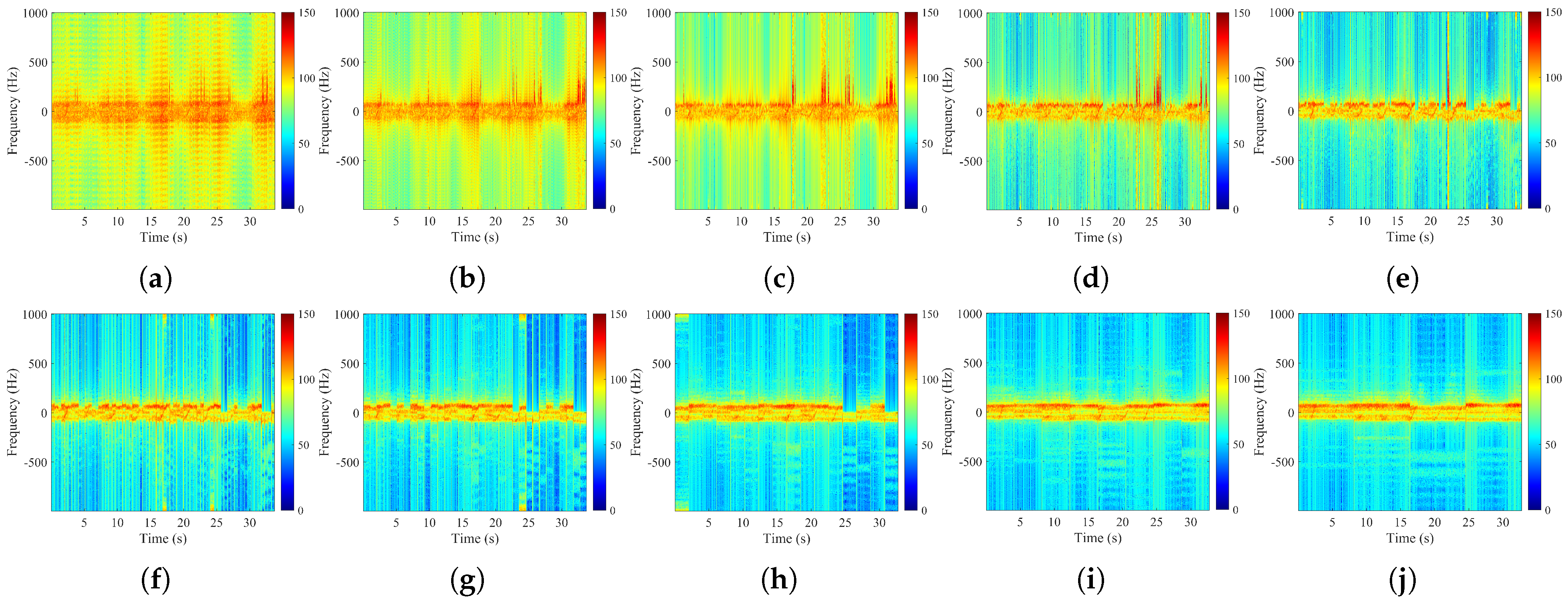
Driven by wind and waves, the buoys drift slowly on the sea surface, resulting in Doppler frequency shifts that fluctuate around zero frequency. Meanwhile, high-sea states push most of the clutter energy toward the low-frequency range. Figure 2 presents the time–frequency spectra of echo signals from different range cells in four representative strong clutter conditions. The data sources and acquisition parameters will be detailed in Section 4. As shown in the figure, the spectral components of the targets and the clutter significantly overlap in the frequency domain.

2.2. Principle of Variational Mode Decomposition

VMD adaptively decomposes the original signal f ( t ) into K IMFs u k ( t ) with minimal bandwidth by solving a variational optimization problem [11]. Each IMF is associated with a center frequency ω k . The fundamental objective is to minimize the total bandwidth of all modes while ensuring that their sum reconstructs the original signal [24].
min { u k } , { ω k } k = 1 K t u k ( t ) e j ω k t 2 2
k = 1 K u k = f ( t )
where t denotes the time derivative operator. To handle the equality constraint, an augmented Lagrangian function is introduced.
L ( { u k } , { ω k } , λ ) = α k = 1 K t u k ( t ) e j ω k t 2 2 + f ( t ) k = 1 K u k ( t ) 2 2 + λ ( t ) , f ( t ) k = 1 K u k ( t )
where α is the frequency penalty parameter, λ is the Lagrange multiplier, and · , · represents the inner product operation. Through alternating updates of u k ( ω ) , ω k , and λ ( t ) , the optimization problem is iteratively solved.
u ^ k ( ω ) = f ^ ( ω ) i k u ^ i ( ω ) + λ ( ω ) 2 1 + 2 α ( ω ω k ) 2
ω k = 0 ω | u ^ k ( ω ) | 2 d ω 0 | u ^ k ( ω ) | 2 d ω
λ ( t ) = λ ( t ) + τ f ( t ) k = 1 K u k ( t )
where τ is the gradient descent learning rate. The iteration process stops when the following conditions are met:
k = 1 K u k n + 1 u k n 2 2 u k n 2 2 < ϵ , n = 1 , 2 , , N
where n is the iteration index, N is the maximum number of iterations, and ϵ is the preset convergence threshold. For VMD implementations, the convergence threshold typically ranges from 10 5 to 10 7 . The optimal threshold value was determined by minimizing the reconstruction error through optimization algorithm within this range. After decomposition, K IMFs u k ( t ) are obtained.

2.3. Multi-Domain Feature Extraction Methods

Common time domain features include Average Amplitude (AA), Peak Height (PH), Temporal Entropy Mean (TEM), and Second-Order Temporal Entropy (SOTE). AA quantifies the mean energy level of the echo in a given range cell [25]. PH measures the prominence of the most significant peaks. TEM reflects the complexity and randomness of the signal, and SOTE captures the variability and dynamics of the entropy over time [26,27].
A A ( x ) = 1 N n = 1 N | x ( n ) |
P H ( x ) = max ( x ) 1 # Δ n Δ + Δ max A ( x Δ )
where # Δ represents the number of elements in the set Δ , and Δ = [ τ 1 , τ 2 ] [ τ 2 , τ 1 ] defines the pulse range involved in the comparison value calculation.
Common frequency domain features include Doppler Peak Height (DPH), Vector Entropy (VE), and Second-Order Frequency Entropy (SOFE). DPH quantifies the prominence of the main peak in the Doppler spectrum. VE and SOFE assess the complexity and dispersion of the signal in the frequency domain [25].
D P H ( x ) = D A S ( f d max , x ) 1 # γ f d f d max + γ D A S ( f d ; x )
D A S ( f d ; x ) = 1 N n = 1 N x ( n ) exp ( 2 π f d n T )
f d max ( x ) = arg max f d D A S ( f d ; x )
where # γ denotes the number of channels, D A S ( f d ; x ) is the Doppler amplitude spectrum in the frequency domain, and γ = [ ϕ 1 , ϕ 2 ] [ ϕ 2 , ϕ 1 ] defines the Doppler channel range over which the ratio is computed.
Common time–frequency domain features include Ridge Integration (RI), Maximal Size of Connected Regions (MS), and Number of Connected Regions (NR). RI integrates the energy along the time–frequency ridge to reinforce the trajectory of the target. MS measures the size of each connected region, reflecting the degree of energy concentration. NR counts the connected regions to characterize the sparsity of the signal [28].
R I ( x , x p ) = n = 1 N N T F D n , arg max f d N T F D ( n , f d | x ; x p ) | x ; x p
N T F D ( n , f d | x ; x p ) = S P W V D ( n , f d | x ) 1 K p = 1 K S P W V D ( n , f d | x p ) 1 K 1 p = 1 K S P W V D ( n , f d | x p ) 1 K p = 1 K S P W V D ( n , f d | x p ) 2
where S P W V D ( n , f d | x ) represents the smoothed pseudo Wigner–Ville distribution (SPWVD) of the detection cell x.
Common time–frequency-ridge transform domain features include the Ridges Radon Transform Maximum Value (RRT-MV) and Ridges Radon Transform Bandwidth (RRT-BW), which characterize the concentration and directionality of the signal in the Radon domain. Given that different features exhibit varying sensitivity and robustness under severe sea clutter, the next chapter will, after presenting the mode selection and reconstruction methods, introduce a dedicated feature evaluation framework.
The multi-domain feature extraction method can comprehensively characterize the multi-scale characteristics of radar echo signals. This approach significantly enhances the detection performance of floating targets in strong sea clutter environments.

3. Spectral Mode Reconstruction Method and Evaluation Framework

The SMR method builds on the results of VMD decomposition and utilizes prior information of floating targets and background sea clutter to formulate an adaptive selection criterion for the target frequency interval. Subsequently, multi-domain feature extraction is applied to both the original and reconstructed signals. The improvements in target enhancement and clutter suppression are quantitatively assessed using relative feature gain and feature detection probability. The overall process is illustrated in Figure 3.

3.1. Adaptive Selection Criterion for Target Frequency Intervals

To identify and select only those modes that truly contain target information, an effective mode selection criterion must be established. From the target signal perspective, the key spectral characteristic is the Doppler frequency shift in the echo. Floating targets experience radial motion induced by wave action, which leads to frequency deviations in the received signals. The magnitude of the Doppler frequency shift f d is determined by the radial velocity of the floating targets [29,30,31,32].
f d = 2 v r λ T
λ T = c f T X
where v r is positive when the target moves away from the radar and negative when it approaches it. λ T is the signal wavelength, and f T X is the radar carrier frequency. Consequently, the Doppler frequency range of the target is 2 | v r | λ T , 2 | v r | λ T .
On the other hand, clutter spectra are characterized by their spectral centroid and bandwidth. The spectral centroid indicates the center of spectral energy, whereas the bandwidth reflects how widely that energy spreads across frequency. In real ocean conditions, both metrics fluctuate with the sea state. Reliable estimation therefore calls for fitting the clutter spectrum with a suitable distribution model.
This study extracts a large set of spectral–amplitude samples from background range cells and derives the empirical distribution function. Six representative distribution models are fitted to the data, namely the Gaussian, Rayleigh, log-normal, Weibull, K, and exponential distributions. Figure 4 presents the fitting results for the cumulative distribution function (CDF) and the probability density function (PDF) of the clutter data. Visual inspection shows that the log-normal distribution aligns most closely with the empirical distribution. To quantitatively compare the fitting performance of each model, the squared relative error between the theoretical and empirical probability density curves is also illustrated. The log-normal model yields the lowest error among all candidates and is therefore considered the most suitable model for describing sea clutter.
Denote the fitted log-normal distribution parameters by μ and σ . Its probability density function is given by the following equation:
f ( x ) = 1 x σ 2 π exp ( ln x μ ) 2 2 σ 2 , x > 0
where μ and σ are the mean and standard deviation of the log-normal distribution, obtained via maximum likelihood estimation from the clutter data. These fitted parameters are subsequently used to compute the SC and the 3 dB BW.
f 0 = e μ + 1 2 σ 2
BW = e μ σ 2 e σ 2 ln 2 e σ 2 ln 2
By combining the spectrum parameters of the clutter with the Doppler frequency range of the target, an adaptive selection criterion for target frequency intervals is devised.
[ f low , f high ] = f 0 B W 2 , f 0 B W 2 , if   f d < f 0 B W 2 | f d | , | f d | , if   f d f 0 B W 2
The interval criterion is designed based on the relative position between the target Doppler frequency f d and the main clutter energy region. For targets with Doppler frequencies below the lower boundary of the main clutter region f 0 B W 2 , the symmetric interval centered at the clutter boundary preserves target components while maximally suppressing the main clutter zone. When the target Doppler frequency reaches or exceeds this boundary, the interval determined by | f d | ensures complete retention of target frequency components without introducing excessive clutter. This adaptive boundary adjustment achieves optimal clutter suppression while maintaining target signal integrity. Under this criterion, the target spectrum is presumed to lie within the specific interval [ f low , f high ] , while the clutter signal is usually distributed outside this interval. This approach both covers the Doppler frequency shift range of slow-moving floating targets and maximally suppresses clutter, thereby achieving effective separation between target components and clutter components. By examining the center frequency f k of each IMF, it is possible to determine whether it corresponds to the target signal. By summing the IMFs u k ( t ) identified as part of the target signal, the target signal can be reconstructed.
S target ( t ) = k : ω k [ f low , f high ] u k ( t )
where S target ( t ) represents the reconstructed target signal, and ω k is the center frequency of the k-th IMF.
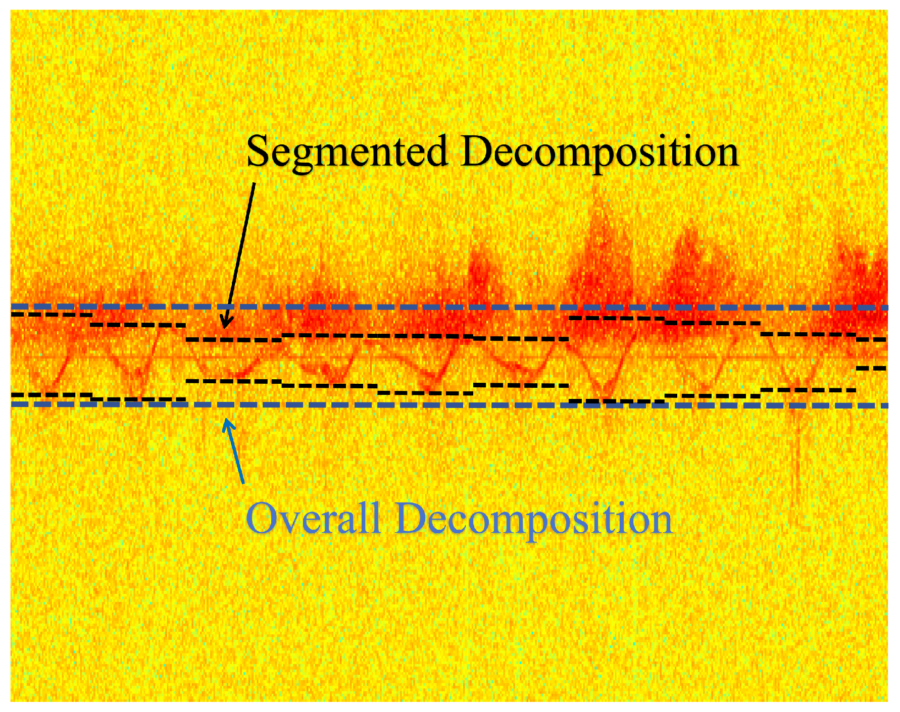
To enhance the separation of target and clutter components, a segmented processing strategy is adopted. The long time-series signal is divided into short segments of length L win , sliding with fixed step size L step . VMD and SMR processing are performed independently within each segment, after which the resulting segments are concatenated to form the complete reconstructed signal. In the overlapping regions of adjacent segments, the corresponding samples are averaged to ensure a smooth transition.
Figure 5 illustrates the schematic comparison between segmented processing and full-length processing. As shown, segmented processing can theoretically preserve nearly the same amount of target signal components while removing more clutter. In contrast, full-length processing requires a longer segment to capture the entire target, which often introduces unnecessary clutter components.

3.2. Relative Feature Gain and Feature Detection Evaluation

To evaluate the effectiveness of the SMR method in simultaneously suppressing clutter and enhancing target returns, a relative feature gain metric is adopted. This metric quantifies, for each feature type, the degree to which the reconstructed signal separates and amplifies target information. The relative feature value R X is defined as follows;
R X = X target X clutter
where X denotes a feature under evaluation, for example, AA, PH, or DPH. X target and X clutter represent the feature values measured in the target range cell and the reference clutter cell, respectively. R X is the corresponding relative feature measure, yielding quantities such as RAA, RPH, and RDPH.
The relative feature gain Δ R X dB is defined to express, on a logarithmic scale, the change in relative feature value between the original signal and the reconstructed signal.
Δ R X dB = 20 log ( R X VMD ) 20 log ( R X 0 )
where R X VMD represents the relative feature value of the reconstructed signal, while R X 0 represents the relative feature value of the original signal.
Effective features are then converted into binary decisions, and performance is quantified by the probability of detecting the target. If each range cell contributes N samples per segment, the total number of segments M is given by the following expression:
M = N L win
For each data segment in every range cell, a detection decision is made by comparing its feature value X to the threshold T. The threshold is determined by analyzing the feature value distribution from a large number of background clutter range cells. Specifically, it is set to exceed 90% of the clutter feature values, ensuring a constant false alarm rate.
D = 1 , if   X > T 0 , if   X T
For a single target range cell, i, its detection probability P d , i is defined as follows:
P d , i = n success , i M
where n success , i represents the number of successful detections of the target in M segments. The overall detection probability P d is the average of the detection probabilities for all target range cells.
P d = 1 K t i = 1 K t P d , i ,
where K t represents the total number of detection opportunities for all targets. The calculation of the overall detection probability provides a comprehensive assessment of the performance the algorithm across all targets.
The relative feature gain Δ R X dB exhibits a positive correlation with detection probability P d . This relationship stems from the reduced overlap between target and clutter feature distributions when Δ R X dB increases, which enhances detectability under constant false-alarm-rate constraints.
This study also incorporates classical non-coherent and coherent integration detection methods to further validate the SMR method. Notably, non-coherent integration detection is fundamentally equivalent to AA feature detection, as both rely on the amplitude statistics.
Coherent integration detection applies a p-point FFT to the multi-pulse echo sequence within each segment for each range cell, yielding a frequency domain representation | Z ( f ) | and allowing the magnitudes of its frequency components to be computed [33].
| Z ( f ) | = R ( Z ( f ) ) 2 + I ( Z ( f ) ) 2
where R ( Z ( f ) ) and I ( Z ( f ) ) represent the real and imaginary parts of Z ( f ) , respectively. The frequency domain signal is divided into p Doppler channels, and the target signal is detected by analyzing the amplitude of each frequency sampling point [34]. A coherent integration threshold, G 0 , is set, requiring the target signal to be detected in a series of consecutive Doppler channels to confirm the range cell as the target [35].

4. Experimental Data Sources and Parameter Settings

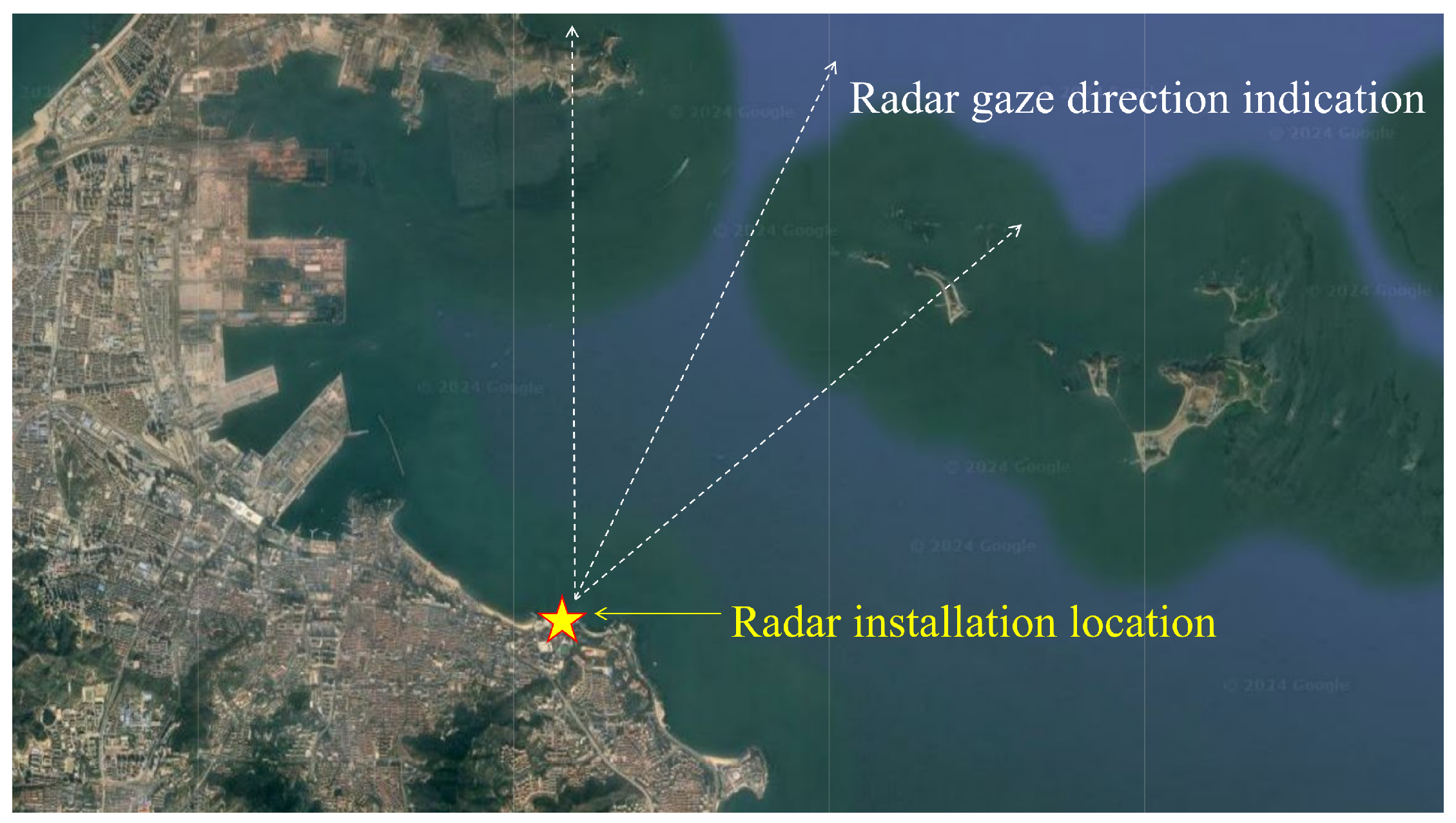
The data used in this study are sourced from the Sea-Detecting Radar Data-Sharing Program (SDRDSP) [36,37,38,39]. Measurements were carried out at the First Bathing Beach in Yantai City, China, as shown in Figure 6. The data were collected using two SPPR50P X-band experimental radars equipped with solid-state power amplifiers, as shown in Figure 7. The specific radar parameter configurations are listed in Table 1.
The operating frequency range of the radar is from 9.3 GHz to 9.5 GHz. This study uses the center frequency of 9.4 GHz for calculation. The estimated radial velocity of the buoys is approximately 0.8 m/s. The calculated wavelength is approximately 0.0319 m. The Doppler frequency range is approximately −50.16 Hz to 50.16 Hz.
Four datasets were used to validate the proposed SMR method, labeled as 2022112175025_stare_VV, 2022112180016_stare_HH, 2022112300011_stare_VV, and 2022112140039_stare_HH, corresponding to Data Group 1–4, respectively. The data cover sea state levels 4 and 5, with wave heights ranging from 1.8 m to 2.7 m. The detailed parameters of these four datasets are presented in Table 2.
For each of the four data groups, a reference clutter range cell was selected to calculate the SC and 3 dB BW. These values, together with the Doppler shift range of the buoy targets, were used to establish the thresholds for the target frequency interval. The specific parameters are given in Table 3.
Based on the four experimental datasets, extensive parameter tuning was carried out to ensure effective detection of both strong and weak targets. The number of IMFs K was set to 25 to capture a broad range of frequency components and more effectively separate target echoes from background clutter. The frequency penalty parameter α was chosen as 665.02, and the gradient-descent learning rate τ was set to 0.00114 to stabilize Lagrange multiplier updates and promote smooth convergence. A convergence threshold of 1 × 10 5 was imposed so that iterations terminated once the relative change in the modal spectra fell below this value, ensuring decomposition accuracy. To guard against non-convergence, the maximum number of iterations N was limited to 5000.

5. Experimental Results and Analysis

This section begins by evaluating the performance of full-length processing and extracting multi-domain features from both the original and reconstructed signals to identify the most discriminative metrics. It then investigates the impact of different segment lengths on reconstruction quality, determining the optimal processing segment size. Finally, the reconstructed signals are assessed using relative feature gain and target detection probability.

5.1. Results and Analysis of Mode Decomposition and Reconstruction

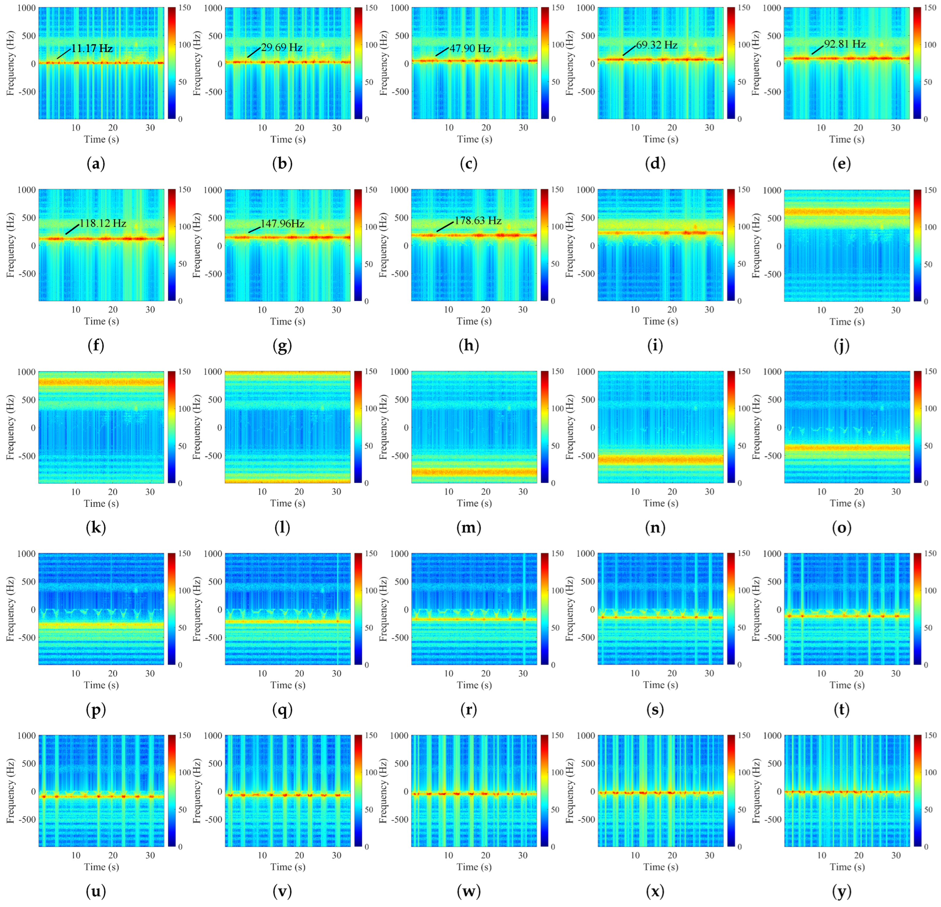
To demonstrate the effectiveness of spectral mode reconstruction, the echo signal from a strong target range cell in Data Group 1 was processed using full-length variational mode decomposition, and the time–frequency spectrogram of each mode is presented in Figure 8. Each IMF was then classified according to the adaptive target frequency interval selection criterion, with the outcomes summarized in Table 4. Modes 1–4 and Modes 22–25 exhibit center frequencies tightly clustered in a low-frequency narrow band, matching the expected Doppler characteristics of the buoys, and are therefore identified as target modes. The remaining modes primarily correspond to background sea clutter and noise.
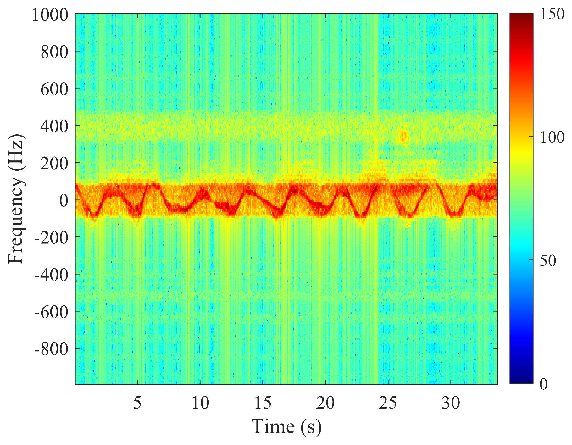
Summing the identified target modes yields the reconstructed signal, as shown in Figure 9. Compared with the original echoes, the reconstructed signal exhibits a tighter concentration of energy in the time–frequency plane, with sea clutter markedly suppressed.

5.2. Feature Extraction and Selection for Reconstructed Signals

For each of the four data groups, a strong target range cell, a weak target range cell, and a reference clutter range cell were selected. The strong and weak target range cells correspond to the center and boundary range cell in Table 3, respectively. The central cells exhibit stronger returns due to complete target illumination. The boundary cells show weaker signals because the target is off the center of the beam’s illumination, causing the target’s echo energy to be much lower than it would be at the center of the beam. Multi-domain features were extracted from both the original and the reconstructed signals, and their relative values were computed. The results are presented in Table 5, Table 6, Table 7, Table 8, Table 9, Table 10, Table 11 and Table 12.
The comparison reveals that RAA, RPH, RDPH, and RRI show marked enhancements in strong target range cells, with RAA, RPH, and RDPH consistently outperforming. Among frequency-domain features, RI responds most prominently to the target signal. By contrast, SOTE and SOFE offer limited discrimination and lack stability. Furthermore, comparative analysis across different sea states reveals that the relative feature values of effective features under sea state 4 conditions generally surpass those under sea state 5 conditions. Notably, RAA, RPH, and RDPH values in Data Group 4 reach approximately 10. These findings align with the fundamental theory governing sea state and detection performance; higher sea states correspond to increased clutter intensity, consequently elevating the difficulty of target detection.
Balancing feature performance with computational cost is also crucial for real applications. Denoting the length of the signal by N, this study uses O -notation to assess each feature’s complexity and measures their extraction times on the reconstructed signals from Data Group 1, as shown in Table 13. AA and PH incur the lowest complexity, each requiring a single pass over N samples. DPH, which involves an FFT and bandwidth calculation, carries moderate complexity but remains acceptable. RI must iterate through every sample and perform frequency domain operations, resulting in a runtime that is orders of magnitude longer than the other three features.

5.3. Determining the Optimal Processing Segment Length

The segmented processing strategy was applied to track target signal fluctuations more precisely within shorter intervals. Mode decomposition and reconstruction were performed on four datasets using segment lengths ranging from 32 to 16,384 pulses, with no overlap between adjacent segments. The features were extracted from each segment, and the average feature value across all segments served as the evaluation metric. Figure 10 shows the reconstructed signals at different segment lengths. The observed trends are consistent with the schematic in Figure 5.
The results demonstrate that segment length has a significant impact on the reconstruction. For short segments of 32 and 64 pulses, the time–frequency representation is relatively sparse, emphasizing local details. However, some frequency components are lost due to the limited segment length. For moderate segments of 256, 512, and 1024 pulses, the time–frequency distribution becomes balanced. The regions of concentrated target energy are clearly defined, and the time–frequency pattern closely matches the target signature. For long segments of 8192 and 16,384 pulses, increasing the segment length smooths the frequency distribution but at the expense of finer details.
AA, PH, and DPH, previously selected for their high gain and low cost, were extracted and averaged across segments. Table 14 and Table 15 summarize the relative feature values and the relative feature gains for each segment length. Figure 11 visualizes the effect of segment length on the relative feature gains.
The results indicate that segment lengths of 256 and 512 pulses deliver the best overall performance, with particularly notable gains in Δ RAA ¯ d B and Δ RPH ¯ d B . Although gains continue to rise beyond 512 pulses, the improvement begins to level off. When the segment length reaches 16,384 pulses, the enhancement oscillates and even declines.
From a practical standpoint, segment length must align with the pulse repetition frequency of the radar. When a 256-pulse segment corresponds to about 0.128 s, meeting real-time processing requirements while striking a good balance between feature enhancement and computational complexity is imperative. Through experimental analysis of four distinct data groups, this optimal segment length was rigorously established for floating targets in strong clutter environments. It should be emphasized that the parameter may require adaptation for different operational scenarios, particularly when processing weaker clutter conditions or faster-moving targets, as these variations significantly impact the time–frequency characteristics of both target signatures and clutter components.
To investigate the impact of overlap ratio on target and clutter discrimination, feature performance was evaluated for four overlap ratios, namely 0%, 25%, 50% and 75%, in segmented processing. Table 16 lists the RAA, RPH, and RDPH values at each overlap ratio, and Table 17 shows the corresponding relative feature gains.
As shown in the table, non-overlapping segments deliver the greatest feature improvement. Overlapping segments spread the target signal across multiple segments, averaging its energy and reducing its prominence. They also introduce additional background clutter, which degrades feature extraction. In addition, increasing the overlap ratio significantly raises computational complexity while the performance gains plateau or even decline.
Based on experimental results and considering practical performance and application requirements, a non-overlapping segmented processing strategy using 256-pulse segments was chosen as the optimal mode decomposition and reconstruction approach.

5.4. Feature Detection Results and Evaluation

After extracting AA, PH, and DPH from both the original signal and the reconstructed signal obtained via non-overlapping 256-pulse segmented processing, feature detection and coherent integration detection were applied separately to each dataset to assess the practical performance of the SMR method for floating target detection under strong clutter.
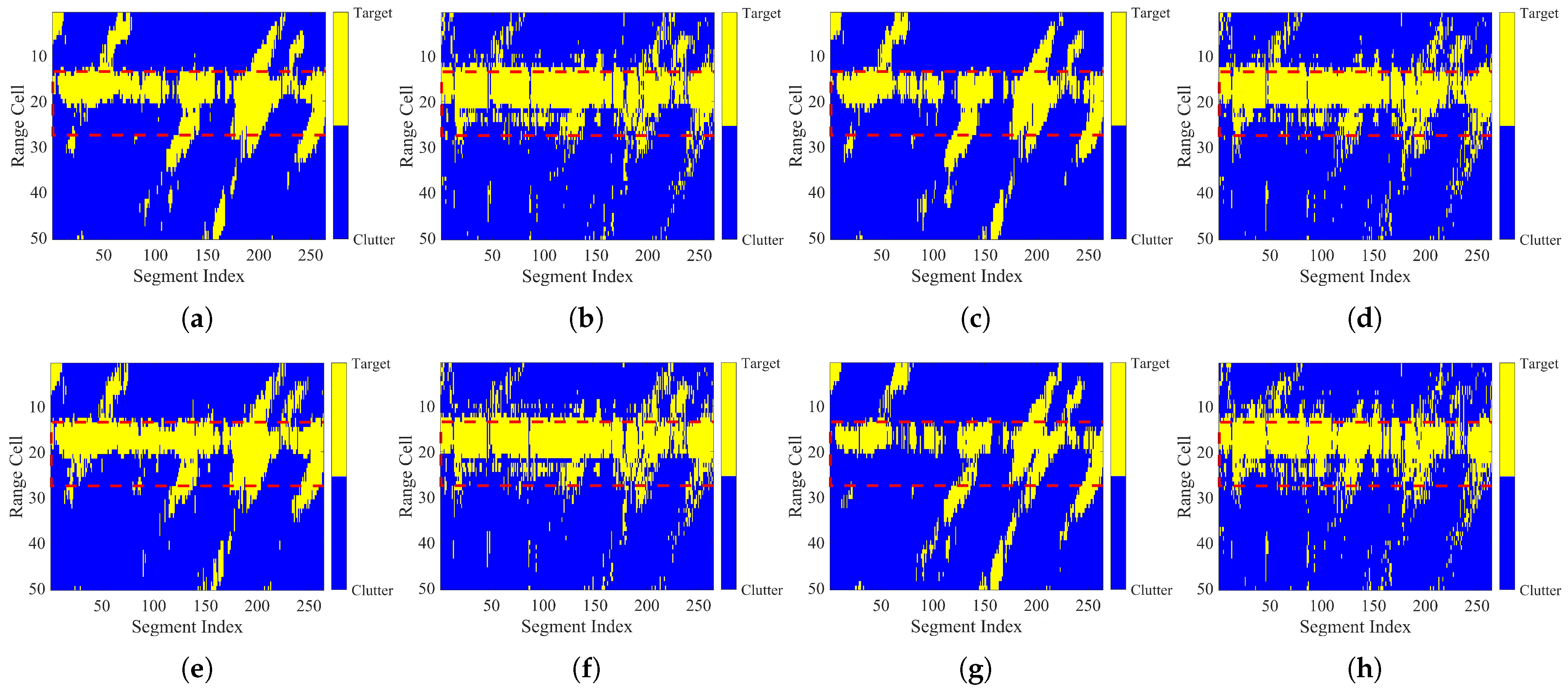
Figure 12 shows the detection results of the three feature-based methods and the coherent integration method on both the original and reconstructed signals under the same false alarm rate. The horizontal axis represents segment index and the vertical axis represents the range cell index. In the reconstructed signal results, the detected region within the target cells is more complete, and missed detections are greatly reduced.
Figure 13 presents the target detection probability statistics for different target range cells using each detection method. It can be seen that, for every method, the reconstructed signal achieves higher overall detection probabilities than the original signal, with the greatest gains occurring at strong target range cells. Table 18 lists the average detection probability across all target range cells for each method and gives the percentage increase of the reconstructed signal over the original, further confirming the clear advantage of the SMR method.

6. Conclusions

This paper presents a spectral mode reconstruction method for floating target signal under strong sea clutter. The proposed method uses an adaptive selection criterion for target frequency intervals to accurately identify and reconstruct target modes, effectively suppressing sea clutter and enhancing target characteristics. Compared with the original signals, the reconstructed signals demonstrate significant increases in relative feature gain and target detection probability. Moreover, determining the optimal processing segment length proved critical for maximizing clutter suppression. Looking ahead, modal decomposition and reconstruction can be combined with more target-discriminative features and deployed in more complex sea conditions and multi-target scenarios to further enhance sea clutter suppression.

Author Contributions

Conceptualization, N.L. and H.Y.; methodology, N.L. and H.Y.; software, H.Y. and G.W.; validation, H.Y. and H.D.; formal analysis, H.Y. and N.L.; investigation, H.Y. and N.L.; resources, W.X. and Y.D.; data curation, H.Y. and N.L.; writing—original draft preparation, H.Y.; writing—review and editing, N.L. and W.X.; visualization, H.Y. and G.W.; supervision, N.L. and W.X.; project administration, N.L. and Y.D.; funding acquisition, N.L. and Y.D. All authors have read and agreed to the published version of the manuscript.

Funding

This research was supported by the National Natural Science Foundation of China (Grant No.62388102 and Grant No.62101583).

Data Availability Statement

The data supporting the findings of this study are openly available and can be accessed upon request or through the public release by the authors.

Conflicts of Interest

The authors declare no conflicts of interest.

References

  1. Serafino, F.; Bianco, A. X-Band Radar Detection of Small Garbage Islands in Different Sea State Conditions. Remote Sens. 2024, 16, 2101. [Google Scholar] [CrossRef]
  2. Feintuch, S.; Permuter, H.H.; Bilik, I.; Tabrikian, J. Neural network-based multitarget detection within correlated heavy-tailed clutter. IEEE Trans. Aerosp. Electron. Syst. 2023, 59, 5684–5698. [Google Scholar] [CrossRef]
  3. Wu, H.; Guo, H.; Wang, Z.; He, Z. Rao and Wald tests in nonzero-mean non-Gaussian sea clutter. Remote Sens. 2025, 17, 1696. [Google Scholar] [CrossRef]
  4. Wen, B.; Lu, Z.; Zhou, B.; Mao, Y. Background clutter modeling of spatio-temporal sea clutter suppression for low grazing angle X-Band marine radar. In Proceedings of the OCEANS 2024, Halifax, NS, Canada, 23–26 September 2024; pp. 1–5. [Google Scholar] [CrossRef]
  5. Wen, B.; Wei, Y.; Lu, Z. Sea clutter suppression and target detection algorithm of marine radar image sequence based on spatio-temporal domain joint filtering. Entropy 2022, 24, 250. [Google Scholar] [CrossRef]
  6. Huang, P.; Yang, H.; Xia, X.-G.; Zou, Z.; Liu, X.; Liao, G. A novel sea clutter rejection algorithm for spaceborne multichannel radar systems. IEEE Trans. Geosci. Remote Sens. 2022, 60, 5117422. [Google Scholar] [CrossRef]
  7. Randall, R.B.; Antoni, J. Why EMD and Similar Decompositions Are of Little Benefit for Bearing Diagnostics. Mech. Syst. Signal Process. 2023, 192, 110207–110227. [Google Scholar] [CrossRef]
  8. Shamaee, Z.; Mivehchy, M. Dominant noise-aided EMD (DEMD): Extending empirical mode decomposition for noise reduction by incorporating dominant noise and deep classification. Biomed. Signal Process. Control 2023, 80, 104218–104230. [Google Scholar] [CrossRef]
  9. Khaled, M.L.; Tarhini, A.A.; Forsyth, P.A.; Smalley, I.; Piña, Y. Leptomeningeal Disease (LMD) in Patients with Melanoma Metastases. Cancers 2023, 15, 1884. [Google Scholar] [CrossRef]
  10. Zhang, K.; He, W.; Liu, L.; Gao, K. Sea clutter denoising based on complete ensemble empirical mode decomoposition. In Proceedings of the 2022 4th International Conference on Natural Language Processing (ICNLP), Xi’an, China, 25–27 March 2022; pp. 282–286. [Google Scholar] [CrossRef]
  11. Ahmadi, F.; Tohidi, M.; Sadrianzade, M. Streamflow prediction using a hybrid methodology based on variational mode decomposition (VMD) and machine learning approaches. Appl. Water Sci. 2023, 13, 135–152. [Google Scholar] [CrossRef]
  12. Qin, C.; Huang, G.; Yu, H.; Zhang, Z.; Tao, J.; Liu, C. Adaptive VMD and multi-stage stabilized transformer-based long-distance forecasting for multiple shield machine tunneling parameters. Autom. Constr. 2024, 165, 105563–105583. [Google Scholar] [CrossRef]
  13. Zhao, L.; Li, Z.; Qu, L.; Zhang, J.; Teng, B. A hybrid VMD-LSTM/GRU model to predict non-stationary and irregular waves on the east coast of China. Ocean Eng. 2023, 276, 114136–114153. [Google Scholar] [CrossRef]
  14. Jiang, S.; Xing, H.; Wu, J. Distributed sea clutter denoising algorithm based on variational mode decomposition. Instrumentation 2020, 7, 23–32. [Google Scholar]
  15. Nie, T.; Li, J.; Ding, Y.; Zhang, Z.; Li, B.; Dong, W. Fast extraction for Brillouin frequency shift in BOTDA system. Opt. Quant. Electron. 2021, 53, 73–81. [Google Scholar] [CrossRef]
  16. Li, Z.; Zhao, Y.; Hu, X.; Botta, N.; Ionescu, C.; Chen, G.H. ECOD: Unsupervised outlier detection using empirical cumulative distribution functions. IEEE Trans. Knowl. Data Eng. 2023, 35, 12181–12193. [Google Scholar] [CrossRef]
  17. Liao, X.; Xie, J.; Zhou, J. Compound Gaussian radar clutter model with positive tempered alpha-stable texture. arXiv 2024, arXiv:2412.05174. [Google Scholar] [CrossRef]
  18. Zhu, M.-X.; Shao, Y.-H. Classification by estimating the cumulative distribution function for small data. IEEE Access 2023, 11, 41142–41157. [Google Scholar] [CrossRef]
  19. Sørensen, K.A.; Heiselberg, P.; Heiselberg, H. Unified detection and feature extraction of ships in satellite images. Remote Sens. 2024, 16, 4719. [Google Scholar] [CrossRef]
  20. Xiong, G.; Wang, L.; Yu, W. Radar sea clutter reconstruction based on statistical singularity power spectrum and instantaneous singularity exponents distribution. IEEE Trans. Geosci. Remote Sens. 2021, 59, 5687–5697. [Google Scholar] [CrossRef]
  21. Xie, J.; Xu, X. Phase-feature-based detection of small targets in sea clutter. IEEE Geosci. Remote Sens. Lett. 2022, 19, 3507405. [Google Scholar] [CrossRef]
  22. Guo, Z.-X.; Shui, P.-L.; Bai, X.-H. Small target detection in sea clutter using all-dimensional Hurst exponents of complex time sequence. Digit. Signal Process. 2020, 101, 102707–102715. [Google Scholar] [CrossRef]
  23. Fan, S.; Zhang, B.; Kudryavtsev, V. Comprehensive assessment of ocean surface current retrievals using SAR Doppler shift and drifting buoy observations. Remote Sens. 2025, 17, 2007. [Google Scholar] [CrossRef]
  24. Yang, D.; Guo, C.; Persico, R.; Liu, Y.; Liu, H.; Bai, C.; Lian, C.; Zhao, Q. Adaptive variational mode decomposition and principal component analysis-based denoising scheme for borehole radar data. Remote Sens. 2025, 17, 525. [Google Scholar] [CrossRef]
  25. Shui, P.-L.; Li, D.-C.; Xu, S.-W. Tri-feature-based detection of floating small targets in sea clutter. IEEE Trans. Aerosp. Electron. Syst. 2014, 50, 1416–1430. [Google Scholar] [CrossRef]
  26. Yu, W.; Yang, G.; Zhao, H. A new method for ship length estimation based on Doppler spectrum analysis. Radar Sci. Technol. 2015, 13, 522–526. [Google Scholar]
  27. Guan, J.; Jiang, X.; Liu, N.; Ding, H.; Dong, Y.; Liu, T. Target detection in sea clutter based on feature re-expression using Spearman’s correlation. IEEE Sens. J. 2024, 24, 30435–30450. [Google Scholar] [CrossRef]
  28. Wu, X.-J.; Ding, H.; Liu, N.-B.; Guan, J. A method for detecting small targets in sea surface based on ridges-Radon transform. J. Signal Process. 2021, 37, 1599–1611. [Google Scholar]
  29. Wen, C.; Huang, Y.; Davidson, T.N. Efficient transceiver design for MIMO dual-function radar-communication systems. IEEE Trans. Signal Process. 2023, 71, 1786–1801. [Google Scholar] [CrossRef]
  30. Wen, C.; Huang, Y.; Zheng, L.; Liu, W.; Davidson, T.N. Transmit waveform design for dual-function radar-communication systems via hybrid linear-nonlinear precoding. IEEE Trans. Signal Process. 2023, 71, 2130–2145. [Google Scholar] [CrossRef]
  31. Wen, C.; Huang, Y.; Peng, J.; Wu, J.; Zheng, G.; Zhang, Y. Slow-time FDA-MIMO technique with application to STAP radar. IEEE Trans. Aerosp. Electron. Syst. 2021, 58, 74–95. [Google Scholar] [CrossRef]
  32. Wen, C.; Chen, Y.; Huang, Y.; Davidson, T.N. Reduced-Complexity CRB Optimization for Dual-Function Radar-Communication Systems using Hybrid Linear-Nonlinear Precoding. IEEE Trans. Signal Process. 2025, 73, 2123–2138. [Google Scholar] [CrossRef]
  33. Liu, C.; Li, P.; Liu, L.; Li, Q.; Liu, Y. Multi-Strategy Constant False Alarm Rate Detector in Complex Backgrounds. In Electronic Engineering and Informatics; Advances in Transdisciplinary Engineering; IOS Press: Amsterdam, The Netherlands, 2024; Volume 51, pp. 77–85. [Google Scholar] [CrossRef]
  34. Kuang, C.; Wang, C.; Wen, B.; Hou, Y.; Lai, Y. An improved CA-CFAR method for ship target detection in strong clutter using UHF radar. IEEE Signal Process. Lett. 2020, 27, 1445–1449. [Google Scholar] [CrossRef]
  35. Ge, Y.; Huang, Z.-Z.; Liu, Q.; Lan, Q. Fast implementation of CA-CFAR algorithm based on FFT. In Proceedings of the 2021 IEEE 5th Advanced Information Technology, Electronic and Automation Control Conference (IAEAC), Chongqing, China, 12–14 March 2021; pp. 2494–2498. [Google Scholar] [CrossRef]
  36. Guan, J.; Liu, N.; Wang, G.; Ding, H.; Dong, Y.; Huang, Y.; Tian, K.; Zhang, M. Sea-detecting radar experiment and target feature data acquisition for dual polarization multistate scattering dataset of marine targets. J. Radars 2023, 12, 456–469. [Google Scholar] [CrossRef]
  37. Liu, N.; Ding, H.; Huang, Y.; Dong, Y.; Wang, G.; Dong, K. Annual progress of the sea-detecting X-band radar and data acquisition program. J. Radars 2021, 10, 173–182. [Google Scholar] [CrossRef]
  38. Liu, N.; Dong, Y.; Wang, G.; Ding, H.; Huang, Y.; Guan, J.; Chen, X.; He, Y. Sea-detecting X-band radar and data acquisition program. J. Radars 2019, 8, 656–667. [Google Scholar] [CrossRef]
  39. Liu, N.; Li, J.; Wang, G.; Chen, B.; Cao, Z.; Dong, Y.; Guan, J.; Jiang, X.; Zhang, Z.; Xue, W. Sea-detecting radar experiment and target feature data acquisition for multisource observation dataset of maritime targets. J. Radars 2025, 14, 754–780. [Google Scholar] [CrossRef]
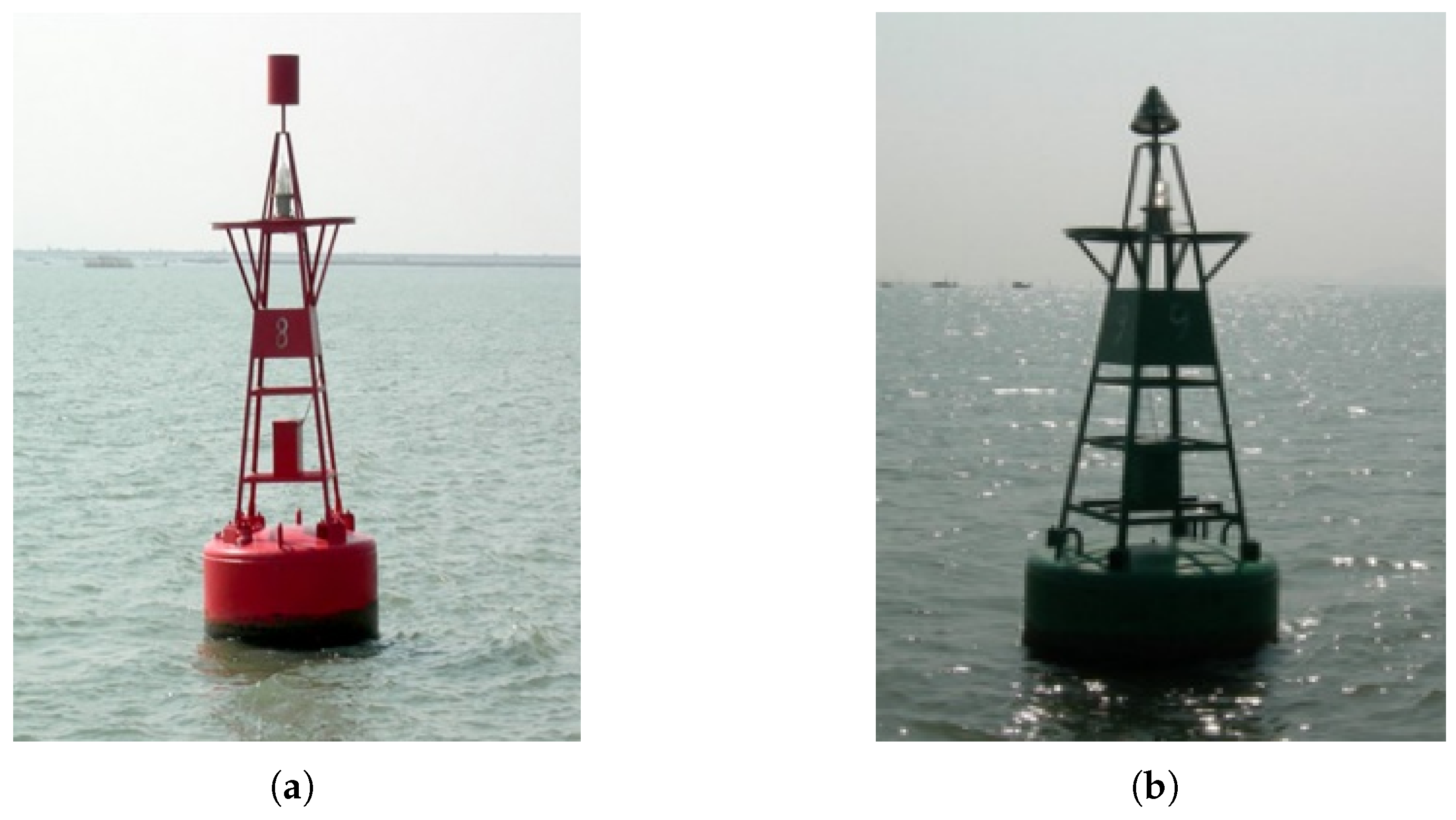
Figure 1. Channel buoy. (a) Buoy 1. (b) Buoy 2.
Remotesensing 17 03155 g001
Figure 2. Time-frequency spectrograms from different range cells across the four data groups. (a) Strong target range cell in Data Group 1. (b) Weak target range cell in Data Group 1. (c) Reference clutter range cell in Data Group 1. (d) Strong target range cell in Data Group 2. (e) Weak target range cell in Data Group 2. (f) Reference clutter range cell in Data Group 2. (g) Strong target range cell in Data Group 3. (h) Weak target range cell in Data Group 3. (i) Reference clutter range cell in Data Group 3. (j) Strong target range cell in Data Group 4. (k) Weak target range cell in Data Group 4. (l) Reference clutter range cell in Data Group 4.
Remotesensing 17 03155 g002
Figure 3. Overall flowchart of the proposed method.
Remotesensing 17 03155 g003
Figure 4. Comparison of fitting results for various distribution models. (a) Cumulative distribution function fit comparison. (b) Probability density function fit comparison. (c) Squared relative error comparison.
Remotesensing 17 03155 g004
Figure 5. Illustration of segmented processing.
Remotesensing 17 03155 g005
Figure 6. Data collection location.
Remotesensing 17 03155 g006
Figure 7. Configuration and display interface of two X-band fully coherent solid-state radars. (a) HH-polarized radar antenna. (b) VV-polarized radar antenna. (c) HH-polarized radar display interface. (d) VV-polarized radar display interface.
Remotesensing 17 03155 g007
Figure 8. Time-frequency spectrograms of different IMFs. (a) IMF 1. (b) IMF 2. (c) IMF 3. (d) IMF 4. (e) IMF 5. (f) IMF 6. (g) IMF 7. (h) IMF 8. (i) IMF 9. (j) IMF 10. (k) IMF 11. (l) IMF 12. (m) IMF 13. (n) IMF 14. (o) IMF 15. (p) IMF 16. (q) IMF 17. (r) IMF 18. (s) IMF 19. (t) IMF 20. (u) IMF 21. (v) IMF 22. (w) IMF 23. (x) IMF 24. (y) IMF 25.
Remotesensing 17 03155 g008
Figure 9. Time-frequency spectrogram of reconstructed signal.
Remotesensing 17 03155 g009
Figure 10. Time-frequency spectrograms of reconstructed signals with different segment lengths. (a) Segment Length 32. (b) Segment Length 64. (c) Segment Length 128. (d) Segment Length 256. (e) Segment Length 512. (f) Segment Length 1024. (g) Segment Length 2048. (h) Segment Length 4096. (i) Segment Length 8192. (j) Segment Length 16,384.
Remotesensing 17 03155 g010
Figure 11. Average relative feature gain across different segment lengths. (a) Data Group 1. (b) Data Group 2. (c) Data Group 3. (d) Data Group 4.
Remotesensing 17 03155 g011
Figure 12. Detection results of different methods. (a) Original signal AA detection results. (b) Reconstructed signal AA detection results. (c) Original signal PH detection results. (d) Reconstructed signal PH detection results. (e) Original signal DPH detection results. (f) Reconstructed signal DPH detection results. (g) Original signal coherent integration detection results. (h) Reconstructed signal coherent integration detection results.
Remotesensing 17 03155 g012
Figure 13. Detection probability comparison of different methods across target range cells.
Remotesensing 17 03155 g013
Table 1. Radar parameter configuration table.
CategoryParameter/InformationValue/Description
Experimental ConditionsExperiment LocationYantai First, Seaside Bathing Beach Test Site
Maximum Wave Height2.8 m
Maximum Wind Speed16.7 m/s
Radar ModelSPPR50PSolid-State Amplification Monitoring/Navigation Radar
Polarization statesHH/VVHorizontal–Horizontal/Vertical–Vertical Polarization
Radar ParametersOperation ModeStaring/Scanning
Frequency BandX Band
Working Frequency9.3 GHz–9.5 GHz
Pulse Duration40 ns–100 μ s
Transmission Power100 W
Range Resolution6 m
Pulse Repetition Frequency2000 Hz
Target TypeLight BuoysRed Cylindrical Buoy 1, Green Cylindrical Buoy 2
Buoy LocationDistance to Buoy 12.97 nautical miles
Distance to Buoy 23.19 nautical miles
Table 2. Experimental data parameters.
DataSeaPolarizationEffective WaveWaveCollectionRange DimensionTargetTargetPulse
GroupStateModeHeight (m)DirectionDuration (s)Sample CountRange CellCount
15VV2.7North–65.51000Buoy 1494–50667,584
NorthwestBuoy 2663–676
25HH2.7North–65.51000Buoy 1496–50867,584
Northwest
34VV2.3North–65.51000Buoy 1492–502131,072
NortheastBuoy 2663–674
44HH1.8North–65.51000Buoy 1498–506131,072
NorthwestBuoy 2666–674
Table 3. Target and clutter range cell parameters.
DataCenterBoundaryReference ClutterClutter SpectralClutter 3 dBReconstructed
GroupRange CellRange CellRange CellCentroid (Hz)Bandwidth (Hz)Threshold (Hz)
1670676691123.2798.1074.22
2502508523171.19109.85116.27
3669674689117.1570.6781.82
4670674689145.7790.27100.64
Table 4. Frequency characteristics of different IMFs.
IMFCenter Frequency (Hz)Bandwidth (Hz)Target IMF
111.1732.47Yes
229.6931.73Yes
347.9021.07Yes
469.3224.45Yes
592.8123.14No
6118.1224.14No
7147.9629.25No
8178.6334.30No
9229.8761.96No
10605.1884.48No
11799.71130.68No
12−185.94956.11No
13−789.43118.24No
14−577.3273.87No
15−366.4051.83No
16−281.3667.79No
17−218.5550.79No
18−178.4341.73No
19−149.8638.59No
20−121.9035.38No
21−97.2729.74No
22−72.0123.55Yes
23−48.9325.45Yes
24−29.9024.43Yes
25−9.4222.70Yes
Table 5. Feature extraction results of original signal for Data Group 1.
FeatureStrong Target
Range Cell
Weak Target
Range Cell
Clutter
Range Cell
Relative Value
(Strong Target Cell)
Relative Value
(Weak Target Cell)
AA 6.877 × 10 4 3.293 × 10 4 3.154 × 10 3 2.1801.044
PH 3.355 × 10 5 2.618 × 10 5 2.181 × 10 5 1.5391.201
TEM3.3903.3543.3541.0111.000
SOTE 2.683 × 10 3 2.127 × 10 3 2.314 × 10 3 1.1600.919
DPH 1.815 × 10 8 1.252 × 10 8 1.713 × 10 8 1.0600.731
VE 1.009 × 10 1 1.033 × 10 1 1.034 × 10 1 0.9750.999
SOFE 5.817 × 10 2 5.190 × 10 2 5.541 × 10 2 1.0500.937
RI 4.332 × 10 15 1.432 × 10 15 1.244 × 10 15 3.4841.151
NR 7.721 × 10 4 1.055 × 10 5 1.099 × 10 5 0.7030.960
MS 2.550 × 10 2 2.550 × 10 2 2.520 × 10 2 1.0121.012
RRT_BW 2.010 × 10 2 3.570 × 10 2 4.130 × 10 2 0.4870.864
RRT_MV 2.259 × 10 3 2.602 × 10 3 2.748 × 10 3 0.8220.947
Table 6. Feature extraction results of reconstructed signal for Data Group 1.
FeatureStrong Target
Range Cell
Weak Target
Range Cell
Clutter
Range Cell
Relative Value
(Strong Target Cell)
Relative Value
(Weak Target Cell)
AA 4.517 × 10 4 5.782 × 10 3 6.859 × 10 3 6.5860.843
PH 1.968 × 10 5 3.453 × 10 4 5.560 × 10 4 3.5400.621
TEM3.4223.4003.4131.0030.996
SOTE 2.666 × 10 3 2.951 × 10 3 2.245 × 10 3 1.1881.315
DPH 1.548 × 10 8 4.445 × 10 7 5.903 × 10 7 2.6220.753
VE 8.873 × 10 1 8.374 × 10 1 8.171 × 10 1 1.0861.025
SOFE 1.470 × 10 1 1.826 × 10 1 1.371 × 10 1 1.0721.332
RI 1.389 × 10 15 2.751 × 10 13 3.697 × 10 13 37.5960.744
NR 2.432 × 10 4 2.200 × 10 4 2.226 × 10 4 1.0920.988
MS 2.560 × 10 2 2.560 × 10 2 2.560 × 10 2 1.0001.000
RRT_BW 6.590 × 10 2 1.267 × 10 3 1.481 × 10 3 0.4450.856
RRT_MV 5.412 × 10 3 8.989 × 10 3 1.059 × 10 4 0.5110.849
Table 7. Feature extraction results of original signal for Data Group 2.
FeatureStrong Target
Range Cell
Weak Target
Range Cell
Clutter
Range Cell
Relative Value
(Strong Target Cell)
Relative Value
(Weak Target Cell)
AA 1.261 × 10 4 1.147 × 10 4 1.018 × 10 4 1.2401.127
PH 1.012 × 10 5 9.763 × 10 4 1.304 × 10 5 0.7760.749
TEM3.3663.3613.3581.0031.001
SOTE 2.454 × 10 3 2.432 × 10 3 2.881 × 10 3 0.8520.844
DPH 5.103 × 10 8 4.471 × 10 7 5.843 × 10 7 0.8730.765
VE 1.152 × 10 1 1.153 × 10 1 1.151 × 10 1 1.0011.002
SOFE 4.035 × 10 3 4.010 × 10 3 4.450 × 10 3 0.9070.901
RI 3.537 × 10 14 3.082 × 10 14 2.765 × 10 14 1.2791.115
NR 3.246 × 10 5 3.231 × 10 5 3.318 × 10 5 0.9780.974
MS 2.500 × 10 2 2.430 × 10 2 2.510 × 10 2 0.9960.968
RRT_BW 2.910 × 10 2 2.610 × 10 3 2.710 × 10 2 1.0740.963
RRT_MV 1.497 × 10 3 1.585 × 10 3 2.150 × 10 3 0.6970.737
Table 8. Feature extraction results of reconstructed signal for Data Group 2.
FeatureStrong Target
Range Cell
Weak Target
Range Cell
Clutter
Range Cell
Relative Value
(Strong Target Cell)
Relative Value
(Weak Target Cell)
AA 4.216 × 10 3 2.546 × 10 3 2.649 × 10 3 1.5910.961
PH 3.702 × 10 4 1.897 × 10 4 2.629 × 10 4 1.4080.722
TEM3.3793.3893.3820.9991.002
SOTE 2.560 × 10 3 2.739 × 10 3 3.762 × 10 3 0.6800.728
DPH 4.234 × 10 7 2.198 × 10 7 2.037 × 10 7 2.0791.079
VE 9.668 × 10 1 9.344 × 10 1 9.616 × 10 1 1.0050.972
SOFE 8.464 × 10 2 9.664 × 10 2 5.724 × 10 2 1.4791.688
RI 3.991 × 10 13 1.321 × 10 13 1.755 × 10 13 2.2740.753
NR 4.219 × 10 4 3.848 × 10 4 7.432 × 10 4 0.5680.518
MS 2.560 × 10 2 2.560 × 10 2 2.560 × 10 2 1.0001.000
RRT_BW 8.930 × 10 2 1.263 × 10 4 2.983 × 10 3 0.2990.423
RRT_MV 5.899 × 10 3 9.414 × 10 3 2.153 × 10 4 0.2740.437
Table 9. Feature extraction results of original signal for Data Group 3.
FeatureStrong Target
Range Cell
Weak Target
Range Cell
Clutter
Range Cell
Relative Value
(Strong Target Cell)
Relative Value
(Weak Target Cell)
AA 6.299 × 10 4 2.856 × 10 4 3.028 × 10 4 2.0800.943
PH 2.432 × 10 5 1.983 × 10 5 2.144 × 10 5 1.1340.925
TEM3.3973.3613.3611.0111.000
SOTE 2.530 × 10 3 2.029 × 10 3 2.256 × 10 3 1.1220.899
DPH 6.375 × 10 8 3.140 × 10 8 4.846 × 10 8 1.3160.648
VE 1.074 × 10 1 1.116 × 10 1 1.105 × 10 1 0.9721.010
SOFE 6.857 × 10 2 3.811 × 10 2 4.660 × 10 2 1.4720.818
RI 5.692 × 10 15 1.586 × 10 15 1.973 × 10 15 2.8850.804
NR 1.872 × 10 5 2.358 × 10 5 2.444 × 10 5 0.7660.965
MS 2.530 × 10 2 2.520 × 10 2 2.530 × 10 2 1.0000.996
RRT_BW 9.550 × 10 2 6.770 × 10 2 8.210 × 10 2 1.1630.825
RRT_MV 7.232 × 10 3 4.842 × 10 3 5.452 × 10 3 1.3260.889
Table 10. Feature extraction results of reconstructed signal for Data Group 3.
FeatureStrong Target
Range Cell
Weak Target
Range Cell
Clutter
Range Cell
Relative Value
(Strong Target Cell)
Relative Value
(Weak Target Cell)
AA 5.080 × 10 4 8.727 × 10 3 9.602 × 10 3 5.2910.909
PH 2.111 × 10 5 4.789 × 10 4 7.752 × 10 4 2.7230.618
TEM3.4323.3983.3931.0111.001
SOTE 2.530 × 10 3 3.381 × 10 3 2.745 × 10 3 0.9221.232
DPH 5.295 × 10 8 2.225 × 10 8 3.996 × 10 8 1.3250.557
VE 9.301 × 10 1 9.301 × 10 1 8.912 × 10 1 1.0441.044
SOFE 1.990 × 10 1 1.542 × 10 1 9.491 × 10 2 2.0961.625
RI 2.811 × 10 15 1.167 × 10 14 1.549 × 10 14 18.1480.753
NR 3.593 × 10 4 4.113 × 10 4 4.259 × 10 4 0.8440.966
MS 2.560 × 10 2 2.560 × 10 2 2.560 × 10 2 1.0001.000
RRT_BW 2.319 × 10 3 2.309 × 10 3 1.941 × 10 3 1.1951.190
RRT_MV 1.622 × 10 4 1.625 × 10 3 1.416 × 10 4 1.1451.147
Table 11. Feature extraction results of original signal for Data Group 4.
FeatureStrong Target
Range Cell
Weak Target
Range Cell
Clutter
Range Cell
Relative Value
(Strong Target Cell)
Relative Value
(Weak Target Cell)
AA 3.350 × 10 4 9.164 × 10 3 7.609 × 10 3 4.4031.204
PH 2.248 × 10 5 7.797 × 10 4 7.893 × 10 4 2.8490.988
TEM3.4133.3573.3581.0161.000
SOTE 2.396 × 10 3 2.107 × 10 3 2.221 × 10 3 1.0790.949
DPH 2.530 × 10 8 4.494 × 10 7 4.543 × 10 7 5.5690.989
VE 1.071 × 10 1 1.113 × 10 1 1.116 × 10 1 0.9600.997
SOFE 1.059 × 10 1 3.736 × 10 1 3.706 × 10 2 2.8581.008
RI 1.651 × 10 15 1.834 × 10 14 1.202 × 10 14 13.7361.526
NR 1.724 × 10 5 2.434 × 10 4 2.755 × 10 5 0.6260.883
MS 2.540 × 10 2 2.520 × 10 2 2.460 × 10 2 1.0331.024
RRT_BW 1.187 × 10 3 3.770 × 10 2 6.510 × 10 2 1.8230.579
RRT_MV 8.663 × 10 3 3.407 × 10 3 4.457 × 10 4 1.9440.764
Table 12. Feature extraction results of reconstructed signal for Data Group 4.
FeatureStrong Target
Range Cell
Weak Target
Range Cell
Clutter
Range Cell
Relative Value
(Strong Target Cell)
Relative Value
(Weak Target Cell)
AA 2.964 × 10 4 2.095 × 10 3 2.325 × 10 3 12.7450.901
PH 2.028 × 10 5 2.226 × 10 4 1.537 × 10 4 13.1911.448
TEM3.4383.4123.4031.0101.003
SOTE 1.993 × 10 3 3.167 × 10 3 2.305 × 10 3 0.8651.374
DPH 2.443 × 10 8 1.919 × 10 7 2.581 × 10 7 9.4640.744
VE 9.339 × 10 1 9.363 × 10 1 9.014 × 10 1 1.0361.039
SOFE 2.703 × 10 1 1.097 × 10 1 6.771 × 10 2 3.9911.620
RI 1.072 × 10 15 6.323 × 10 13 8758 × 10 12 122.4480.722
NR 3.769 × 10 4 4.901 × 10 4 4.162 × 10 4 0.9051.177
MS 2.560 × 10 2 2.560 × 10 2 2.560 × 10 2 1.0001.000
RRT_BW 2.213 × 10 3 1.769 × 10 3 1.903 × 10 3 1.1630.930
RRT_MV 1.568 × 10 4 1.221 × 10 4 1.352 × 10 4 1.1600.904
Table 13. Comparison of computational complexity for AA, PH, DPH, and RI.
FeatureComputationalExecution
ComplexityTime (s)
AA O ( N ) 5.13 × 10 4
PH O ( N ) 2.94 × 10 4
DPH O ( N log N ) 1.05 × 10 3
RI O ( N 2 ) 4.77
Table 14. Average relative feature values under different segment lengths.
Data
Index
SignalRXAll
Pulses
32
Pulses
64
Pulses
128
Pulses
256
Pulses
512
Pulses
1024
Pulses
2048
Pulses
4096
Pulses
8192
Pulses
16,384
Pulses
1Original
Signal
RAA1.04411.64691.61721.59791.58681.58181.56711.53391.39021.05261.0161
RPH1.20051.48171.48331.48421.49741.52281.48861.44501.37501.08200.9839
RDPH0.73062.06412.06942.05792.02131.99391.85571.74821.27791.00760.9041
Reconstructed
Signal
RAA0.84301.74261.91292.08962.21991.86081.56511.39701.30241.39582.2609
RPH0.62112.42232.38042.33162.29612.30842.27562.21342.23102.73992.8035
RDPH0.75302.94362.78432.82252.89402.81512.42232.14801.70281.54311.1476
2Original
Signal
RAA1.12672.24392.19002.15812.14012.12222.09512.03601.90431.51311.1469
RPH0.74881.96051.92381.88951.84271.78731.65311.53691.48381.24031.0053
RDPH0.76522.63222.62312.55072.43452.36502.19552.07041.77671.43100.9677
Reconstructed
Signal
RAA0.96092.72502.45572.38072.43922.36962.23852.10112.06861.44391.0647
RPH0.72162.81442.40672.30062.45382.41722.33212.24482.14291.47450.8907
RDPH1.07912.73472.58672.67222.74392.75032.40572.21462.02661.58501.1447
3Original
Signal
RAA0.94321.35611.32191.29931.28551.27331.26181.23831.17021.06510.9857
RPH0.92481.24001.23311.22331.22241.22811.22141.23111.17141.03510.8966
RDPH0.64801.60351.56161.49931.44911.35241.20681.14920.95520.83420.7050
Reconstructed
Signal
RAA0.90881.57161.57481.60951.63681.89031.42801.27731.31781.28221.2437
RPH0.61791.70111.69621.66321.60391.65801.42191.32831.26421.31781.1358
RDPH0.55681.56331.56281.58021.59741.59551.13290.87380.82160.73250.5884
4Original
Signal
RAA1.20441.52761.48721.45801.43881.42671.41371.39161.35721.31801.2937
RPH0.98781.43111.41761.38631.36101.34261.31181.28841.22901.27141.3689
RDPH0.98931.75451.68901.67731.59601.58171.51151.44731.43231.35811.2852
Reconstructed
Signal
RAA0.90112.05131.81751.72151.66891.64111.62101.59991.57291.56751.5666
RPH1.44812.14051.97971.89311.77641.64271.65101.60141.76051.86901.9817
RDPH0.74352.09722.03092.24212.32792.22842.09231.79781.68131.62001.4278
Table 15. Average relative feature gain under different segment lengths.
Data
Index
Δ RX ¯ dB All
Pulses
32
Pulses
64
Pulses
128
Pulses
256
Pulses
512
Pulses
1024
Pulses
2048
Pulses
4096
Pulses
8192
Pulses
16,384
Pulses
1 Δ RAA ¯ d B −1.85830.49061.45862.33032.91621.4110−0.0111−0.8120−0.56672.45126.9469
Δ RPH ¯ d B −5.72404.26944.10843.92323.71313.61343.68643.70384.20398.07019.0950
Δ RDPH ¯ d B 0.26233.08302.57742.74423.11742.99582.31441.78892.49333.70212.0715
2 Δ RAA ¯ d B −1.38261.68730.99460.85271.13630.95780.57500.27340.7188−0.4066−0.6460
Δ RPH ¯ d B −0.32143.14041.94521.70992.48772.62232.98903.29063.19251.5024−1.0513
Δ RDPH ¯ d B 2.98570.3318−0.12140.40421.03921.31100.79420.58481.14310.88781.4590
3 Δ RAA ¯ d B −0.32271.28101.52051.85962.09853.43201.07480.26931.03181.61132.0194
Δ RPH ¯ d B −3.50262.74622.76962.66822.35932.60701.32020.66010.66222.09732.0541
Δ RDPH ¯ d B −1.3175−0.22050.00670.45650.84631.4358−0.5489−2.3797−1.3087−1.1293−1.5703
4 Δ RAA ¯ d B −2.52002.56041.74211.44301.28861.21601.18851.21161.28111.50581.6625
Δ RPH ¯ d B 3.32263.49692.90092.70632.31371.75221.99761.88903.12173.34653.2133
Δ RDPH ¯ d B −2.48091.54971.60122.52093.27862.97742.82431.88371.39221.53170.9139
Table 16. Effect of segment overlap on relative feature values.
Data
Index
SignalRXNo
Overlap
25%
Overlap
50%
Overlap
75%
Overlap
1Original
Signal
RAA1.58681.58851.58791.5747
RPH1.49740.98390.98390.9839
RDPH2.02132.02872.06301.9762
Reconstructed
Signal
RAA2.21992.23052.19242.0342
RPH2.29610.99521.10061.0473
RDPH2.89402.12872.06142.0033
2Original
Signal
RAA2.14012.14202.14062.1393
RPH1.84271.00531.00531.0053
RDPH2.43452.46642.44062.4688
Reconstructed
Signal
RAA2.43922.38482.38592.3993
RPH2.45381.32241.33421.2806
RDPH2.74392.65592.68452.7006
Table 17. Effect of segment overlap on average relative feature gain.
Data
Index
Δ RX ¯ dB No
Overlap
25%
Overlap
50%
Overlap
75%
Overlap
1 Δ RAA ¯ d B 2.91622.94832.80192.2239
Δ RPH ¯ d B 3.71310.09920.97360.5424
Δ RDPH ¯ d B 3.11740.4179−0.00670.1183
2 Δ RAA ¯ d B 1.13630.93260.94230.9963
Δ RPH ¯ d B 2.48772.38132.45852.1024
Δ RDPH ¯ d B 1.03920.64300.82730.7795
Table 18. Comparison of detection results for original and reconstructed signals.
Detection MethodOriginal SignalReconstructed SignalImprovement
AA Feature Detection0.52540.666126.78%
PH Feature Detection0.47780.658337.78%
DPH Feature Detection0.60200.65809.30%
Coherent Integration Detection0.40370.651561.38%
Disclaimer/Publisher’s Note: The statements, opinions and data contained in all publications are solely those of the individual author(s) and contributor(s) and not of MDPI and/or the editor(s). MDPI and/or the editor(s) disclaim responsibility for any injury to people or property resulting from any ideas, methods, instructions or products referred to in the content.