Interval Determination Strategy for Bayesian Inversion of Seismic Source Parameters Under Uncertain Interval Conditions

Highlights

What are the main findings?

• Two novel strategies—‘CFI’ (Converge First, Then Interval) and ‘IVI’ (Interval Value Iteration)—are proposed to prevent Markov Chain Monte Carlo (MCMC) algorithms from becoming trapped in local optima during the Bayesian inversion of seismic source parameters.
• The ‘IVI’ strategy, when paired with an MCMC algorithm using a normally distribut-ed step size, significantly reduces the root-mean-square error (RMSE) of the inversion results.

What is the implication of the main finding?

• Application to the 2022 Mw6.6 Menyuan earthquake demonstrates the method’s practicality, yielding fault parameters (depth, strike, dip, rake) closer to the GCMT solution with low fitting residuals.
• The strategies provide clear guidance for inversion settings: use ‘IVI’ when parameter ranges are unknown, ‘CFI’ when an approximate range is known, and standard con-straints only when both the interval and a reliable initial model are fully known.

Abstract

Using a Bayesian framework to invert earthquake source parameters from multi-source geodetic data has become an important research direction. To address the issue of Markov Chain Monte Carlo (MCMC) algorithms getting stuck in local optima during nonlinear inversion of fault geometric parameters, which is often caused by improperly set parameter bounds or large deviations in the initial values, this study proposes two strategies: ‘CFI (Converge First, Then Interval)’ and ‘IVI (Interval Value Iteration)’. Tests with 12 different experimental setups show that both strategies can prevent the chain from getting trapped in local optima. Among them, the ‘IVI’ strategy, when used with MCMC algorithms where the step size follows a normal distribution, can also significantly reduce the root-mean-square error. To verify its applicability, the ‘IVI’ strategy was applied to the Bayesian inversion of the 2022 Menyuan Mw6.6 earthquake. The results show that the inverted values for fault depth, strike, dip, and rake angles are closer to the GCMT results, with ascending and descending track fitting residuals of 2.71 cm and 2.64 cm, respectively. The conclusion of this paper is to recommend the ‘IVI’ strategy when the range of source parameters is unclear. If the approximate range of parameters is known, the ‘CFI’ strategy can be applied. The original interval constraint method is recommended when the parameter bounds are fully determinable and a reliable initial model of seismic source parameters is obtainable.

1. Introduction

The use of geodetic methods, such as the Global Navigation Satellite System (GNSS) and synthetic aperture radar interferometry (InSAR), plays an important role in investigating the seismic cycle and the evolution of seismicity. These methods contribute significantly to earthquake forecasting and hazard mitigation [1]. Among them, the use of space geodetic deformation data constraints to invert seismic source parameters, thereby revealing the seismic source mechanism of earthquakes, is a research hotspot in the Earth sciences [2,3,4,5]. In the study of focal mechanism strategy, the dislocation model in elastic half-space (the Okada model) [6] is undoubtedly the simplest and most widely used model. The Okada model provides a complex nonlinear relationship between earthquake source parameters and surface deformation observations. This model enables inversion of earthquake source parameters from multi-source geodetic data. On the basis of this model, many nonlinear intelligent search algorithms or improved algorithms are applied for seismic source parameter inversion. For example, Picozzi et al. [7] used a genetic algorithm (GA) combined with a generalized inversion method to invert the earthquake source parameters of a series of earthquakes in the Geysers geothermal area of California. Yang et al. [8] used the simulated annealing algorithm (SA) and bootstrap method to reverse the source parameters of the 2015 Mw7.8 Gurkha earthquake. Zhao and Xu [9] used an improved Gauss‒Newton method (AMGNA) to invert the 2009 Mw6.3 L’Aquila earthquake and the 2017 Mw6.6 Bodrum‒Kos earthquake. Wang et al. [10] used an improved artificial neural network algorithm to invert the source parameters of the 2017 Mw6.6 Bodrum‒Kos earthquake and the 2020 Mw6.5 Monte Cristo earthquake. However, most nonlinear ‘intelligent’ search algorithms based on natural evolutionary processes share common issues: the optimal parameters they yield exhibit high randomness (i.e., the parameters obtained from the first inversion often differ from those of subsequent inversions) and represent only a relatively optimal strategy for the objective function, often disregarding the inherent uncertainty in seismic inversion.

New methods are urgently needed to overcome the limitations of existing geophysical inversion approaches. Recent advancements in machine learning and improvements in hardware and software have brought the Bayesian algorithm, which is known for its rigorous theoretical foundation, to the forefront. Additionally, the rapid development of space geodesy has provided more accurate prior information and multisource deformation constraints for inferring seismic source parameters [11,12,13]. Because of these conditions, a popular research direction in the fields of geodesy and geophysics in recent years has been accurate source parameter inversion via the Bayesian algorithm [5,13,14,15,16,17,18,19,20,21,22]. Bayesian algorithms for the inversion of seismic parameters are crucial because they account for uncertainty in the results by representing them as a posterior probability density function (PDF). Current research focuses on two key methods: MCMC, which solves the posterior PDF through sampling, and variational Bayesian methods, which address complex integration challenges by approximating the distribution function through optimization.

Currently, the use of MCMC methods is the dominant trend in Bayesian frameworks, and although variational Bayes is more computationally efficient, its complexity and shortcomings limit the use of variational Bayes [21]. In Bayesian algorithms that utilize the MCMC approach, achieving chain convergence during the inversion process critically depends on the choice of prior source parameters and the implementation of interval constraints, which define the feasible range for the parameters and ensure numerical stability and realistic results. Currently, the upper and lower interval constraints for seismic source parameter inversion via geodetic methods are often borrowed from other disciplines or derived from published articles and may lack clear definitions in some cases. If the interval constraints for some parameters are not set appropriately, the Markov chain may frequently hit these limits and oscillate around them, leading to errors in the source parameter inversion (as shown in Figure 1). Moreover, if the interval is set too wide, it can reduce the Markov chain’s convergence speed (Figure 1 shows the incorrect convergence of the Markov chain caused by severely inappropriate settings of the upper and lower bounds for the simulation intervals in the experiments of Section 4). One method is to blindly enlarge the intervals and conduct repeated experiments until a seemingly reasonable result is obtained. However, this approach significantly consumes computational time, inevitably decreases the convergence speed of the Markov chain, and does not guarantee full trust in the inverted parameters.

The development of nonlinear intelligent search algorithms has greatly facilitated the determination of prior values for source parameters [22]. To address the issue of Markov chain oscillation caused by inappropriate interval settings, this paper proposes two strategies. The convergence of the two Bayesian methods of Bagnardi and Hooper [16] and Wang and Xi [22] under different interval constraints and different prior values is tested.

2. Method

2.1. Bayesian Framework

In the Okada model [6], when the source parameters of an earthquake are inverted, the following relationship between space geodetic surface deformation data and the source parameters of an earthquake exists [23,24,25,26]:

$$\mathit{d}=G\left(\mathit{m}\right)+\mathit{\epsilon }$$

(1)

where the data vector $\mathit{d}$ represents the spatial geodetic surface deformation data, $G$ is a nonlinear function model that relates the surface deformation data to the parameters of the seismic source, $\mathit{m}$ represents the earthquake source parameters, which in this paper primarily refer to the parameters involved in the nonlinear inversion of fault geometry, including strike angle, dip angle, fault length, fault width, depth, local coordinates X and Y, as well as the dip-slip and strike-slip components, and $\mathit{\epsilon }$ denotes the geodetic surface deformation data error.

Within the Bayesian framework, the posterior probability density function (PDF) $P\left(\mathit{m}\right|\mathit{d})$, quantifies the conditional probability distribution of seismic source parameters $\mathit{m}$ given the available geodetic observation data. The posterior PDF is mathematically expressed as follows [27]:

$$P(\mathit{m}|\mathit{d})={\displaystyle \frac{P\left(\mathit{d}\right|\mathit{m}\left)P\right(\mathit{m})}{P\left(\mathit{d}\right)}}$$

(2)

where $P\left(\mathit{d}\right|\mathit{m})$ is the likelihood function for the seismic source parameter $\mathit{m}$, given the surface observations $\mathit{d}$, based on the residual between the observed surface observations and the predicted values from the current model. The denominator is a normalized constant that is independent of the seismic source parameter $\mathit{m}$.

In the Bayesian framework, assuming that the geodetic deformation data error $\mathit{\epsilon }$ follows a Gaussian distribution, that its mean value is zero, and that the covariance matrix is ${\mathsf{\Sigma }}_{\mathit{d},\mathit{\epsilon }}\sim N(0,{\mathsf{\Sigma }}_{\mathit{d}})$, the likelihood function formula is as follows [5,16,22]:

$$P(\mathit{d}|\mathit{m})=(2\pi {)}^{-{\displaystyle \frac{D}{2}}}|{\mathsf{\Sigma }}_{\mathit{d}}{|}^{-{\displaystyle \frac{1}{2}}}\times \mathit{exp}[-{\displaystyle \frac{1}{2}}(\mathit{d}-G\mathit{m}{)}^{\mathrm{T}}{\mathsf{\Sigma }}_{\mathit{d}}^{-1}(\mathit{d}-G\mathit{m})]$$

(3)

where $D$ represents the total number of data points and ${\mathsf{\Sigma }}_{\mathit{d}}^{-1}$ represents the reciprocal of the variance‒covariance matrix of a given geodetic dataset $\mathit{d}$. The data vector $\mathit{d}$ can usually consist of one or more datasets (e.g., a combination of multisource spatial geodetic data).

2.2. Principles of MCMC Under the Bayesian Framework

In the process of inverting the seismic source parameters via the Bayesian framework, the posterior PDF is solved via the MCMC method, which can avoid the complex integral calculation of the posterior PDF under the Bayesian framework. By using the Metropolis‒Hastings (MH) algorithm, the sampling can be effectively controlled [16]. After a sufficient number of iterations, the density of the sample is close to the posterior distribution, and a more accurate value than that of the variational Bayesian method is obtained.

In the MH-MCMC method, the initial model parameter ${\mathit{m}}_i$ can be arbitrarily selected, or it can be an a priori value obtained via direct search methods such as nonlinear intelligent search algorithms. In the actual seismic source parameter inversion process, the initial model parameters affect the convergence speed of the Markov chain; i.e., the more reliable the initial model parameter ${\mathit{m}}_i$ is, the faster the Markov chain will enter the stationary distribution and the more reliable the maximum posterior probability solution [22]. This study employs the Multiple Peak Particle Swarm Optimization (MPSO) algorithm to obtain relatively reliable initial values. As an active search algorithm widely adopted in seismic inversion, MPSO operates on principles similar to most intelligent optimization algorithms and features a relatively simple structure. Although the inversion results may exhibit some volatility, they remain comparatively reliable [22].

One step within the range of $P\left(\mathit{m}\right)$ is advanced by generating a new set of model parameters on the basis of the actual step size generated randomly (the result of multiplying the initial step size by a random step). If the priors of each of the model parameters are consistent and independent of each other, this is achieved by perturbing each of the parameters in ${\mathit{m}}_i$. The random sampling step $\Delta {\mathit{m}}^j$ of the Bayesian method of Bagnardi and Hooper [16] tested in this paper is a uniformly distributed random value generated in the range [−1, 1]. The $\Delta {\mathit{m}}^j$ of the Bayesian method of Wang and Xi [22] is a random value that conforms to the normal distribution generated in the range [−1, 1]. $\Delta {\mathit{m}}^j$ is the maximum random walking step size of each parameter ${\mathit{m}}^j$. The final value of the step size depends on the product of the current $\Delta {\mathit{m}}^j$ and the set initial step size. If any model parameter of the new model trial is outside the range of the uniform prior probability, the value of ${\mathit{m}}_{TRIAL*}^j$ will be replaced by the following:

$$\left\{\begin{array}{c}{\mathit{m}}_{TRIAL}^j=2\times U{B}^j-{\mathit{m}}_{TRIAL*}^j\\ {\mathit{m}}_{TRIAL}^j=2\times L{B}^j-{\mathit{m}}_{TRIAL*}^j\end{array}\right.\begin{array}{c}if({\mathit{m}}_{TRIAL*}^j>U{B}^j)\\ if({\mathit{m}}_{TRIAL*}^j<L{B}^j)\end{array}$$

(4)

where $U{B}^j$ and $L{B}^j$ are the upper bound and lower bound, respectively, of the interval of the given model parameter ${\mathit{m}}^j$. In the simulation experiment of this paper, the case without an interval constraint is set, which indicates that the case of Equation (4) will not occur in this case. The process of MCMC is shown in Figure 2. It also shows the difference between reasonable interval constraints and unreasonable interval constraints.

2.3. Interval Determination Strategy

To solve the problem of Markov chain oscillation or touching thresholds caused by unreasonable interval setting in seismic source parameter inversion and sampling near the threshold, two interval determination strategies are proposed in this paper.

The first interval determination strategy is named ‘Converge First, Then Interval’ (the abbreviation ‘CFI’ will be used hereafter in this paper to represent this strategy). Interval constraints are not set in the first 20,000 times (sampling times can be changed with seismic complexity); limitations on dip, strike, slip, fault length, fault width, and source depth are specified only by the fault geometry (the dip angle range is 0–90 degrees, the strike angle range is 0–360 degrees, and the slip angle range is −180–180 degrees); and the limiting fault length, fault width, and focal depth are nonnegative. After the Markov chain enters the stationary distribution and is far from the previous oscillation trend, the preset source parameter interval constraint is applied. Bayesian sampling is typically set to 100,000 to 1,000,000 iterations. Therefore, our interval strategy 1 applies the interval constraint after 20,000 samples to achieve the same convergence rate as a reasonable interval. Our interval strategy 1 provides an approach for setting the interval when the general range is roughly known, rather than a strict method. For example, if the constraint is applied after 23,000 samples, theoretically, the convergence speed would not change significantly, as the difference of 3000 samples compared to 1,000,000 is relatively small.

The second interval determination strategy is named ‘Interval Value Iteration’ (The abbreviation “IVI” will be subsequently used in this paper to denote this strategy). The upper and lower limits of the interval change with the change in the source model parameter ${\mathit{m}}_i$. The change Formula (5) is as follows:

$$\left\{\begin{array}{c}U{B}^j={\mathit{m}}_{TRIAL*}^j+a\times \mathit{S}\\ L{B}^j={\mathit{m}}_{TRIAL*}^j-a\times \mathit{I}\mathit{S}\end{array}\right.$$

(5)

In the formula, $a$ is a constant greater than or equal to 1, which can be changed by the specific earthquake period. The goal is to ensure that the next randomized step always lies in the upper and lower bounds of the current interval of strategy 2; that is, when $a$ is greater than or equal to 1, the condition is satisfied. $\mathit{I}\mathit{S}$ is the original step size of the source parameter. These include the fault length, fault width, floor depth, strike angle, dip angle, strike-slip component, dip-slip component, and local X and Y coordinates.

The conversion relationships among the strike-slip component, dip-slip component, slip angle, and slip amount are as follows:

$$\left\{\begin{array}{c}SS=slip\times \mathit{cos}\gamma \\ dS=slip\times \mathit{sin}\gamma \end{array}\right.$$

(6)

where $SS$ is the strike-slip component, $dS$ is the dip-slip component, $slip$ is the slip amount, and $\gamma$ is the slip angle.

The ‘IVI’ method proposed in this study ensures that interval constraints do not hinder the convergence of Markov chains. To validate the adaptability of the interval determination strategy, we examined the convergence of two Bayesian methods: the approach by Bagnardi and Hooper [16] and the method by Wang and Xi [22], under different interval constraints and prior values. The proposed strategy was further applied to invert the source parameters of the 2022 Mw6.6 Menyuan earthquake, which exhibited a steep fault dip angle. Additionally, since the true values of the simulated seismic source parameters were predefined in our synthetic experiments, we introduced the root mean square error (RMSE) to evaluate the convergence of the Markov chains. Specifically:

$$RMSE=\sqrt{{\displaystyle \frac{{\mathit{C}}^T\mathit{C}}{S}}}$$

(7)

In the formula, $\mathit{C}={\mathit{m}}_i-{\mathit{m}}_{true}$ represents the residual of the model parameter ${\mathit{m}}_i$ minus the real value ${\mathit{m}}_{true}$ of the model parameter obtained by each sampling of the Markov chain and $S$ represents the total number of samples.

2.4. Avoiding the Inverse Problem of Deformation Constraints from InSAR Data

In space geodetic observations, the techniques used in interferometric synthetic aperture radar (InSAR) differ from those used in global navigation satellite system (GNSS). Compared to InSAR, GNSS offers more rapid access to three-dimensional co-seismic displacement measurements, but they are generally less accurate in the vertical direction [28]. Many researchers have used GNSS data for fault inversion or slip distribution inversion of seismic sources by removing constraints on vertically oriented displacements [29,30]. Owing to the conversion method of line-of-sight (LOS) deformation and three-direction deformation, the north‒south displacement of InSAR data has fewer constraints on the source parameters. Therefore, to obtain reliable fault data, combining data from multiple sources to constrain the seismic source parameters is highly important [5]. In addition, the combination of GNSS data and InSAR data has a large number of applications in other aspects [31,32,33]. To avoid the inverse problem of LOS deformation of InSAR data to three-direction deformation, the conversion formulas of LOS deformation and three-direction deformation of InSAR data are provided [34,35,36]:

$$\left\{\begin{array}{c}{\mathrm{L}\mathrm{o}\mathrm{o}\mathrm{k}}_E=-sin\theta sin(\alpha -{\displaystyle \frac{3}{2}}\pi )\\ {\mathrm{L}\mathrm{o}\mathrm{o}\mathrm{k}}_N=-\mathit{sin\theta cos}(\alpha -{\displaystyle \frac{3}{2}}\pi )\\ {\mathrm{L}\mathrm{o}\mathrm{o}\mathrm{k}}_U=cos\theta \end{array}\right.$$

(8)

$${\mathit{d}}_{Los}={\mathit{d}}_E{\mathrm{L}\mathrm{o}\mathrm{o}\mathrm{k}}_E+{\mathit{d}}_N{\mathrm{L}\mathrm{o}\mathrm{o}\mathrm{k}}_N+{\mathit{d}}_U{\mathrm{L}\mathrm{o}\mathrm{o}\mathrm{k}}_U$$

(9)

$${\mathit{d}}_{Azi}=-{\mathit{d}}_E\mathit{cos}(\alpha -{\displaystyle \frac{3}{2}}\pi )+{\mathit{d}}_N\mathit{sin}(\alpha -{\displaystyle \frac{3}{2}}\pi )$$

(10)

where $\mathrm{Loo}{\mathrm{k}}_E$, $\mathrm{Loo}{\mathrm{k}}_N$, and $\mathrm{Loo}{\mathrm{k}}_U$ are the angle conversion relationships of the three-direction displacement conversion LOS displacement; $\theta$ is the radar incident angle; $\alpha$ is the satellite heading angle; ${\mathit{d}}_E$, ${\mathit{d}}_N$, and ${\mathit{d}}_U$ are the three-direction displacements of the InSAR data; ${\mathit{d}}_{Los}$ is the line-of-sight displacement; and ${\mathit{d}}_{Azi}$ is the azimuthal displacement.

According to the conversion formula of LOS deformation and three-direction deformation of InSAR data, this paper uses the forward three-direction deformation value of the model parameter ${\mathit{m}}_i$ to calculate the LOS deformation model value and forms a residual with the LOS deformation observation value to meet the calculation requirements of the Bayesian likelihood function, avoiding an inverse problem from LOS deformation to three-direction deformation.

3. Synthetic Experiments

3.1. Synthetic Data

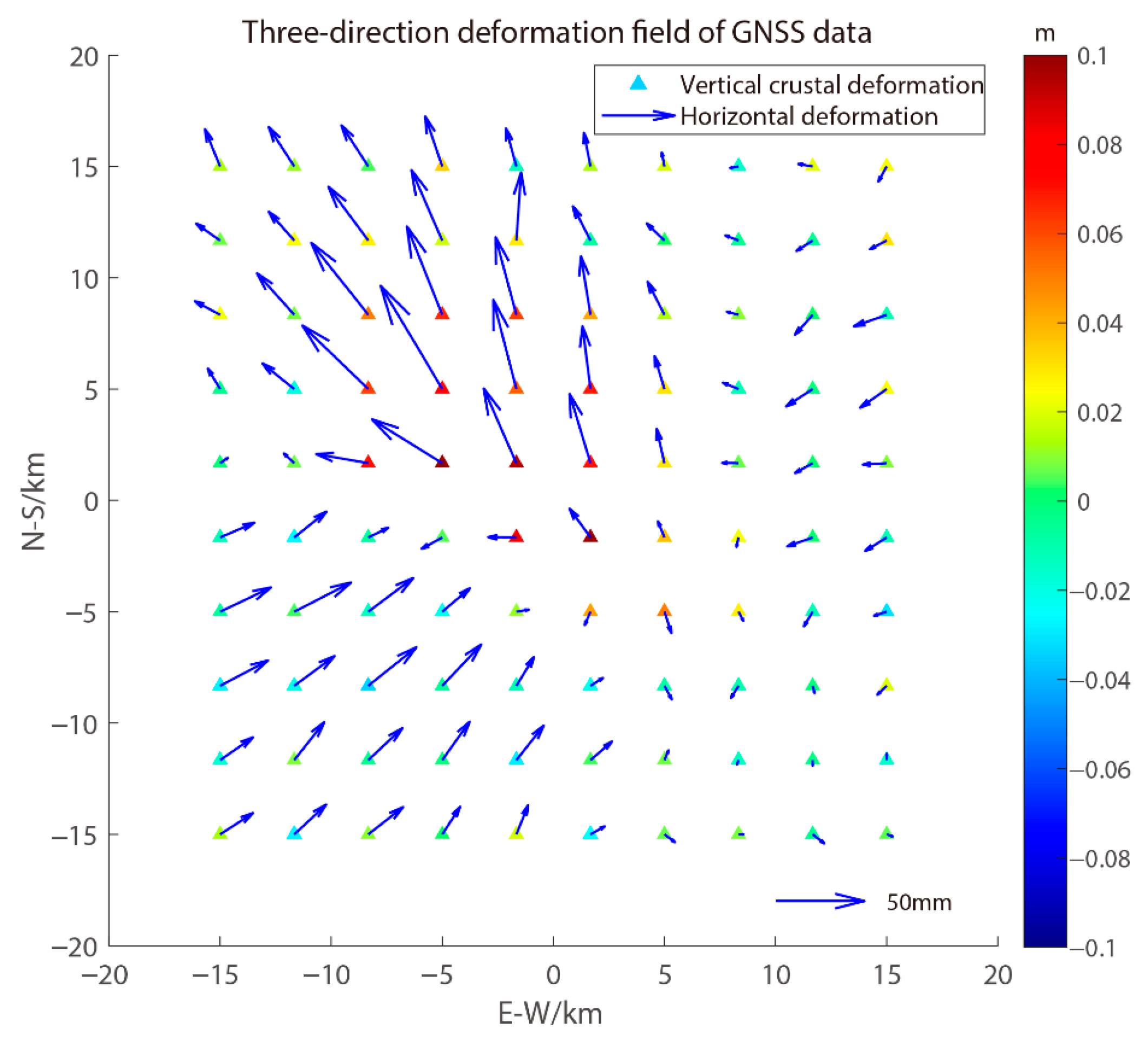
To verify the applicability of the interval determination strategy in seismic source parameter inversion, simulated strike-slip and dip-slip earthquakes are set up in this paper.

Table 1. Inversion interval and prior model settings of the source parameters of the simulated earthquakes.

	Length/m	Width/m	Depth/m	Dip/°	Strike/°	X/m	Y/m	Strike-Slip/m	Dip-Slip/m
lower limit a	10,000	5000	1000	40	280	−20,000	−20,000	0	0
upper limit a	20,000	15,000	18,000	80	340	20,000	20,000	4	4
lower limit b	14,000	9000	11,000	50	290	−3000	−3000	0	0
upper limit b	16,000	11,000	13,000	70	310	3000	3000	0.4	0.4
initial step size of MCMC	100	100	100	1	1	10	10	0.1	0.1
presupposed truth	15,000	10,000	12,330 (bottom depth)	60	300	/	/	0.25712	0.30642
MPSO	14,890	10,030	12,273	57.99	299.74	482.92	157.80	0.25402	0.31246
Random interval generation	15,629	10,812	11,254	68.27	302.65	−2414	−1329	0.21880	0.38300

Note: The upper and lower limits of a refer to the wider interval, and the upper and lower limits of b refer to the narrower interval. The actual step size is equal to the initial step size and random step size. MPSO refers to the source parameters inverted by the MPSO algorithm [37]. Random interval generation means that in a narrow search interval, rand randomly generates a set of parameters to provide initial values for subsequent experiments to simulate the situation in which the initial values are unreliable. The depth in this table is the bottom depth, and the preset true value of the focal depth is 8 km.

shows the preset source parameters. Using the epicenter as the origin, 100 GNSS points in the range of 15 km × 15 km and 10,000 InSAR data points over a 30 km × 30 km area are simulated. On the basis of the preset true values of the simulated earthquake source parameters, the spatial three-direction deformation is obtained via the Okada elastic half-space rectangular dislocation model. In accordance with the practice of Xi et al. [5], normal random errors with specified means and standard deviations are added to the GNSS and InSAR data. In this work, the horizontal deformation of the simulated GNSS data are adjusted with an error of (0 mm, 3² mm²), whereas the vertical deformation includes an error of (0 mm, 15² mm²) to account for data deformation characteristics. The simulated three-dimensional deformation field of the observed volume is shown in Figure 3. For the InSAR data, the simulated satellite azimuth angle is set to −13.11°, with a radar wave incidence angle of 41.69°. Additionally, the InSAR three-dimensional deformation field based on the Okada model was incorporated with normally distributed random errors of (0 mm, 10² mm²). These data are then converted to the LOS displacement field via Equation (8). Figure 4 shows the three-direction and LOS deformation fields before and after the error is applied. Through Equations (8) and (9) in the main text, we converted the three-directional deformation displacement with Gaussian error into the LOS displacement.

3.2. Synthetic Experiment Setup

In this paper, to test the adaptability of the interval determination strategy under different prior values, the nonlinear intelligent search algorithm MPSO (multiple peak particle swarm optimization) [37,38] is used to obtain a set of initial parameters of the model close to the true value, and the MATLAB (2021b) rand command is used to randomly generate a set of model parameters in a narrow interval, as shown in Table 1, to simulate the unreliable initial value. Moreover, this paper sets two sampling intervals, one of which is reasonable and the other is narrow (see Table 1).

To test the convergence of Markov chains under various conditions—including no interval restriction; ‘CFI’; and ‘IVI’—a total of 12 experimental scenarios are set up in this paper. Additionally, the influence of the interval determination strategy on different Bayesian methods is examined. The specific scenarios are detailed in

Table 2. Experimental scheme settings.

Scheme	Algorithm	Interval Constraint	Inversion Initial Value
Scheme 1	Bagnardi and Hooper [16] MCMC algorithm	no interval constraint	MPSO provides the initial value
Scheme 2	Bagnardi and Hooper [16] MCMC algorithm	A reasonable interval constraint	MPSO provides the initial value
Scheme 3	Bagnardi and Hooper [16] MCMC algorithm	narrower interval constraint	random initial value
Scheme 4	Bagnardi and Hooper [16] MCMC algorithm	A reasonable interval constraint (interval determination strategy 1)	MPSO provides the initial value
Scheme 5	Bagnardi and Hooper [16] MCMC algorithm	narrow interval constraint (interval determination strategy 1)	random initial value
Scheme 6	Wang and Xi [22] MCMC algorithm	no interval constraint	MPSO provides the initial value
Scheme 7	Wang and Xi [22] MCMC algorithm	A reasonable interval constraint	MPSO provides the initial value
Scheme 8	Wang and Xi [22] MCMC algorithm	narrower interval constraint	random initial value
Scheme 9	Wang and Xi [22] MCMC algorithm	A reasonable interval constraint (interval determination strategy 1)	MPSO provides the initial value
Scheme 10	Wang and Xi [22] MCMC algorithm	narrow interval constraint (interval determination strategy 1)	random initial value
Scheme 11	Bagnardi and Hooper [16] MCMC algorithm	interval iteratively changed with sampling value (interval determination strategy 2)	random initial value
Scheme 12	Wang and Xi [22] MCMC algorithm	interval iterative change with sampling value (interval determination strategy 2)	random initial value

. Figure 1 shows a failure result from the simulated earthquake experiment. To simulate scenarios where normal/reasonable parameter bounds are unattainable, we deliberately set the upper bound of one parameter to approach (but slightly exceed) the true value, thereby ensuring interval inclusion of the true value. The inversion yielded incorrect results under these conditions. Consequently, such cases were excluded from the 12 experimental scenarios presented in this study. As noted in the Introduction (and demonstrated in Figure 1), inversion failures or errors may occur when standard parameter bounds cannot be established. The objective of the 12 experiments in this paper is to explore the presentation between more moderate situations and normal methods, which better reflects the benefits of the method presented, rather than to perform a comparison with the results that are bound to fail or be incorrect (the experimental situation in Figure 1 is not an entirely extreme case because in a truly extreme case, the bounds would not contain the correct value; imagine that these inversion results would inevitably be incorrect).

To improve the inversion efficiency, this paper adopts a variance-based sampling method for the simulated InSAR data. A total of 10,000 points are used for quadtree downsampling [39], resulting in 133 InSAR points after sampling. The distribution of the sampled points is shown in Figure 3. Additionally, the constant (a) in Equation (10) is 3 (which is greater than 1).

3.3. Synthetic Experiment Results

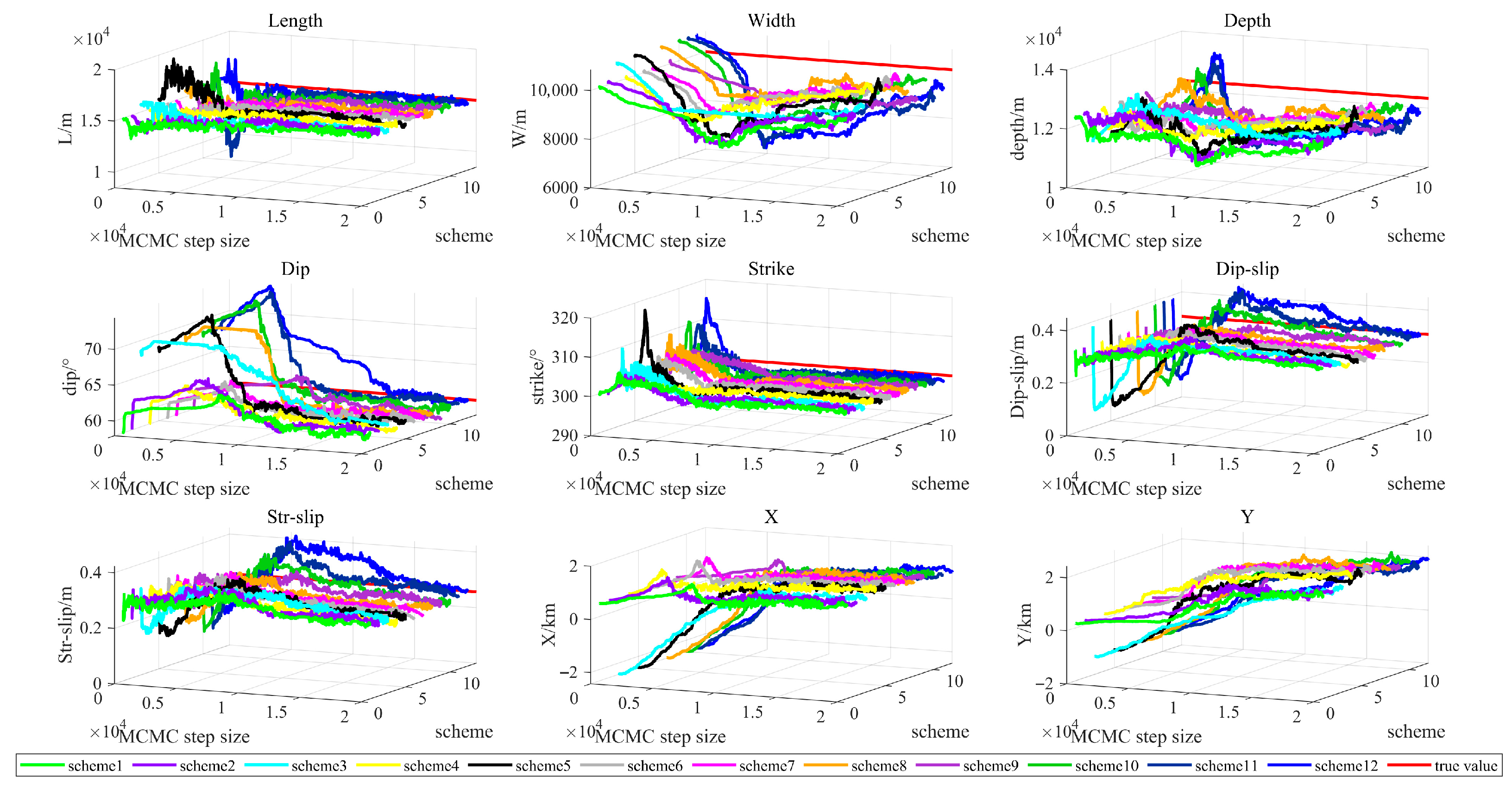
The simulated seismic source parameters obtained by the 12 schemes in 1 million samples of the Bayesian MCMC algorithm are shown in Table S1. In this paper, the RMSE is used to measure the deviation of each sampling point of the Markov chain from the true value. Concerning Formula (12), the RMSE of 1 million sampling points of the Markov chain of the 12 schemes deviates from the true value, as shown in

Table 3. RMSE of 1 million sampling points of the Markov chain from the true value.

RMSE of Each Scheme	Length/m	Width/m	Depth/m	Dip/°	Strike/°	Strike-Slip/m	Dip-Slip/m
Scheme 1	240.99	218.15	198.00	7.57	6.70	1.43	1.22
Scheme 2	244.99	141.17	136.35	7.77	6.59	1.67	1.50
Scheme 3	244.42	214.99	193.69	8.06	6.24	1.38	1.14
Scheme 4	239.31	157.78	155.56	8.28	6.57	1.64	1.47
Scheme 5	246.91	147.46	149.84	9.32	6.83	1.63	1.43
Scheme 6	236.44	175.04	117.06	8.35	6.76	1.72	1.56
Scheme 7	236.44	175.04	117.06	8.35	6.76	1.72	1.56
Scheme 8	243.34	181.78	172.65	8.49	6.27	1.50	1.27
Scheme 9	239.78	170.92	163.69	7.96	6.58	1.56	1.38
Scheme 10	243.62	187.45	169.92	8.80	6.39	1.58	1.40
Scheme 11	255.42	302.41	214.35	13.36	8.01	2.15	1.95
Scheme 12	251.28	169.82	153.65	9.68	6.32	1.61	1.36

Note: The data from Schemes 6 and 7 are identical. This may occur because the MCMC step size in the Bayesian algorithm proposed by Wang and Xi [22] follows a normal distribution overall, resulting in generally small step sizes. Consequently, the range of step size activity shows no clear constraint relationship with the predefined parameter intervals.

. Simultaneously, to better analyze the RMSE of the variation from the true value after the Markov chain enters the stationary distribution, this paper removes the RMSE of the variation from the true value of the Markov chain of the first 200,000 sampling points of the 12 systems, as shown in

Table 4. RMSE of 800,000 sample points from the true value after removal of the Markov chain of the first 200,000 points.

RMSE of Each Scheme	Length/m	Width/m	Depth/m	Dip/°	Strike/°	Strike-Slip/m	Dip-Slip/m
Scheme 1	243.56	184.98	176.64	7.91	6.70	1.47	1.28
Scheme 2	247.98	133.66	137.66	7.70	6.62	1.65	1.48
Scheme 3	251.23	209.39	195.19	7.75	6.96	1.42	1.22
Scheme 4	241.86	186.35	178.05	8.31	6.57	1.58	1.38
Scheme 5	249.87	136.78	146.11	8.24	6.87	1.62	1.43
Scheme 6	239.87	177.11	119.60	8.29	6.82	1.74	1.58
Scheme 7	239.87	177.11	119.60	8.29	6.82	1.74	1.58
Scheme 8	246.08	182.77	176.22	7.91	6.63	1.51	1.33
Scheme 9	239.68	158.43	155.32	7.96	6.54	1.56	1.39
Scheme 10	243.91	156.81	127.54	8.23	6.75	1.68	1.54
Scheme 11	259.03	310.69	224.00	12.32	8.08	2.17	1.99
Scheme 12	238.64	117.80	128.03	8.08	6.77	1.60	1.42

Note: The data from Schemes 6 and 7 are identical. This may occur because the MCMC step size in the Bayesian algorithm proposed by Wang and Xi [22] follows a normal distribution overall, resulting in generally small step sizes. Consequently, the range of step size activity shows no clear constraint relationship with the predefined parameter intervals.

. Figure 4, Figures S1 and S2 show the first 20,000 Markov chain sampling maps, the first 500,000 Markov chain sampling maps, and the last 500,000 Markov chain sampling maps of the 12 schemes.

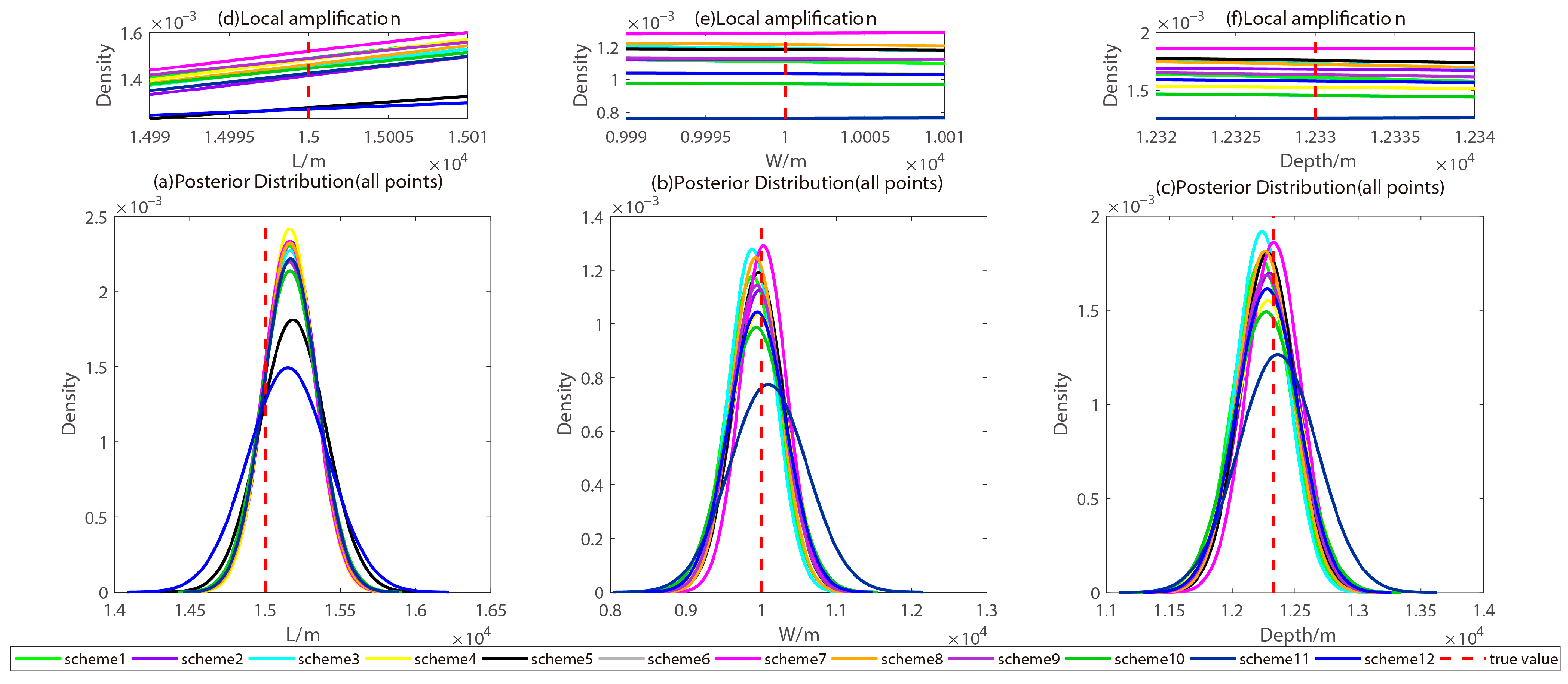
To emphasize the differences in the parameters (including fault length, width, depth, dip angle, strike angle, dip-slip component, and strike-slip component) of the Markov chains for each scheme, posterior probability distribution plots for all 12 schemes (Figure 5 and Figure 6), posterior probability distribution plots for the first 20,000 points (Figures S3 and S4), the first 200,000 points (Figures S5 and S6), and the last 800,000 points (Figures S7 and S8) are presented in this paper. Each figure also includes zoomed-in subplots for the respective parameters.

Table 3 and Table 4, as well as Figure 5, Figures S1 and S2, compare the RMSE of the Markov chain deviation from the true values of the length, width, depth, dip angle, strike angle, strike-slip component, and dip-slip component of the 12 schemes. The width, bottom depth, strike-slip component, and dip-slip component of the simulated earthquake have larger oscillation amplitudes than the other parameters during sampling.

Table 3 shows that when the interval setting is reasonable and the initial model parameters are close to the true value, the Markov chains of the two Bayesian methods of Bagnardi and Hooper [16] and Wang and Xi [22] are closer to the true value. In the Bayesian method of Bagnardi and Hooper [16], the RMSE values of Schemes 5 and 4 are only slightly higher than the reasonable interval. When the reasonable interval is unknown, interval determination strategy 1 of ‘CFI’ can effectively increase the convergence speed of the Markov chain and make it enter the stationary distribution. Even if the initial model parameters deviate from the true value, the interval determination strategy 1 can effectively increase the convergence speed of the Markov chain. According to Scheme 11, because the step size of Bagnardi and Hooper [16] obeys a uniform distribution and the overall step size is large, interval determination strategy 2 of ‘IVI‘ may not be suitable for Bagnardi and Hooper [16]. This may also be because the initial value model parameters of Scheme 11 deviate far from the true value.

In the Bayesian method of Wang and Xi [22], the MCMC step size conforms to the normal distribution, and the step size is more inclined to approach the true value. Interval determination strategy 2 of ‘interval values iterative‘ and interval determination strategy 1 of ‘CFI‘ are also adapted to the Bayesian method of Wang and Xi [22] when the initial value model parameters deviate far from the true value. However, the Bayesian method of Wang and Xi [22] needs to conform to the normal distribution because the MCMC step size needs to conform to the normal distribution. Therefore, each sampling method involves one more multiplication than the Bayesian method of Wang and Xi [22]. For the 1 million samples, the Bayesian method of Wang and Xi [22] takes slightly more time than the Bayesian method of Bagnardi and Hooper [16], which takes approximately 10–20 s.

Figure 5 and Figures S1–S4 show that in some scenarios with significantly deviating initial values, the Markov chain shows noticeable oscillation during the early sampling phase. Table 4, which excludes the first 200,000 points, reveals that the root mean square errors (RMSEs) for the last 800,000 sampling points across the 12 schemes significantly decrease for both the Bayesian MCMC algorithms of Bagnardi and Hooper [16] and Wang and Xi [22] when the “CFI” strategy 1 is used. This finding indicates that interval determination strategy 1 effectively adapts to both Bayesian algorithms.

In Scheme 12, which employs the ‘IVI’ strategy 2 combined with the Bayesian MCMC algorithm by Wang and Xi [22], the root mean square error (RMSE) deviating from the true value is the smallest among the 12 schemes. This finding demonstrates that interval determination strategy 2 is significantly more effective under the Bayesian MCMC algorithm of Wang and Xi [22], outperforming strategy 1. Additionally, the zoomed-in posterior probability distribution plots for the parameters of the Markov chains in Figure 6, Figure 7, and Figures S3–S7 further support this conclusion.

When the Bayesian MCMC algorithm of Wang and Xi [22] is combined with scheme 12 of the interval iteration of interval determination strategy 2, the RMSE of the deviation from the true value is the smallest of the 12 schemes. Interval determination strategy 2 is effective under the Bayesian MCMC algorithm of Wang and Xi [22] and is superior to interval determination strategy 1.

4. Application of the Menyuan Earthquake

4.1. Background

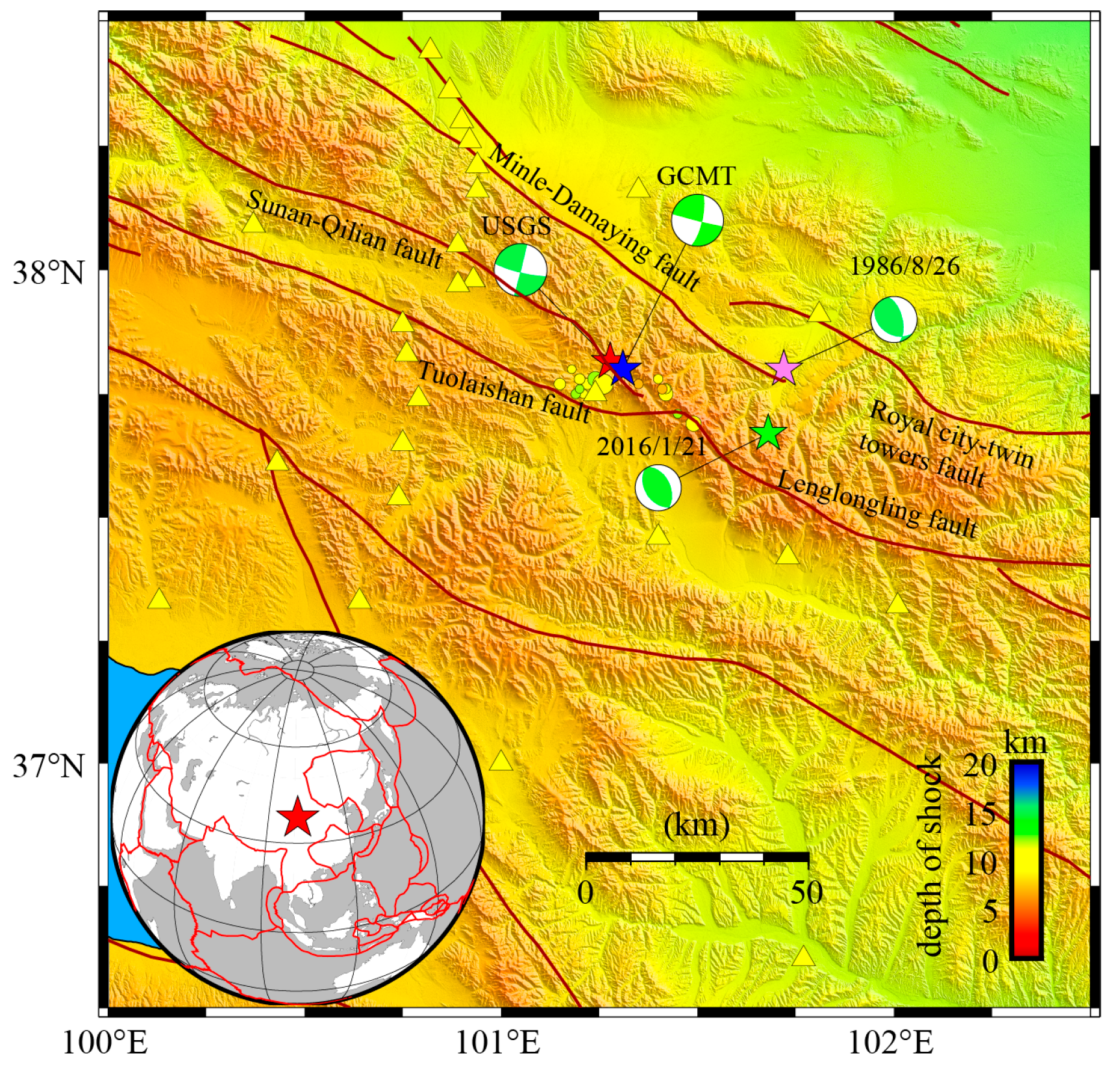
At 1:45 a.m. on 8 January 2022 (URT + 8, Chinese standard time), an earthquake of Mw6.6 occurred at 101.26°E, 37.77°N, north of Huangcheng Township, Menyuan County, Haibei Prefecture, Qinghai Province, in the Tibetan Plateau region of China [40]. The focal depth of the earthquake was 10 km, according to the China Seismological Network (https://news.ceic.ac.cn/, accessed on 7 September 2025). This earthquake and its aftershocks have been named the Menyuan earthquake by the scientific community. The western part of the Lenglongling fault of the Qilian–Haiyuan fault zone was the epicenter of the earthquake. The Mw5.9 earthquake on 26 August 1986 and the Mw5.9 earthquake on 21 January 2016 occurred in this area. The North Lenglongling Fault, a few kilometers from the Lenglongling Fault, is the seismic source of the 1986 and 2016 earthquakes [41,42,43,44,45,46,47]. Xu et al. [40] reported that the magnitude of the Menyuan earthquake in the western section of the Lenglongling fault was too small, which was lower than the expected magnitude of the large earthquake hazard area in this area [48]. Attention still needs to be paid to future seismic hazards in the central section of the Lenglongling fault.

After the earthquake, numerous researchers have investigated the seismogenic fault model of the Menyuan earthquake using diverse datasets and research objectives. While these fault models exhibit certain discrepancies, they consistently indicate that the Menyuan earthquake occurred on a steeply dipping fault, with dip angles predominantly exceeding 80° and approaching vertical [49,50,51,52,53,54]. In this case, if the interval constraints and initial model parameters are unreasonable, the Bayesian MCMC algorithm is likely to become trapped near the upper and lower bounds of the allowable range for the source parameters, resulting in sampling that remains close to these bounds. Ultimately, incorrect or failed inversion results are obtained. In this context, to verify the applicability of the interval determination strategy in this paper for actual complex earthquakes, the MCMC algorithm under the Bayesian framework of Wang and Xi [22] and interval determination strategy 2 are used to invert the source parameters of the Menyuan earthquake. Moreover, a set of MATLAB rand function values is used to simulate the case in which the initial value is not reliable, that is, Scheme 12 in the simulation experiment. The Menyuan earthquake source map is shown in Figure 7. Owing to the limited number of GPS stations for the source earthquakes in this dataset, as shown in Figure 7, there is a scarcity of near-field GPS stations at the earthquake source [54]. Considering data quality and other factors, refer to the relevant literature [40,43,51] and only use InSAR data for the inversion of the source parameters. In Figure 8, the focal mechanism data for the Mw5.9 earthquake on 26 August 1986 and the Mw5.9 earthquake on 21 January 2016 are sourced from the GCMT agency.

4.2. Data and Model Set Up

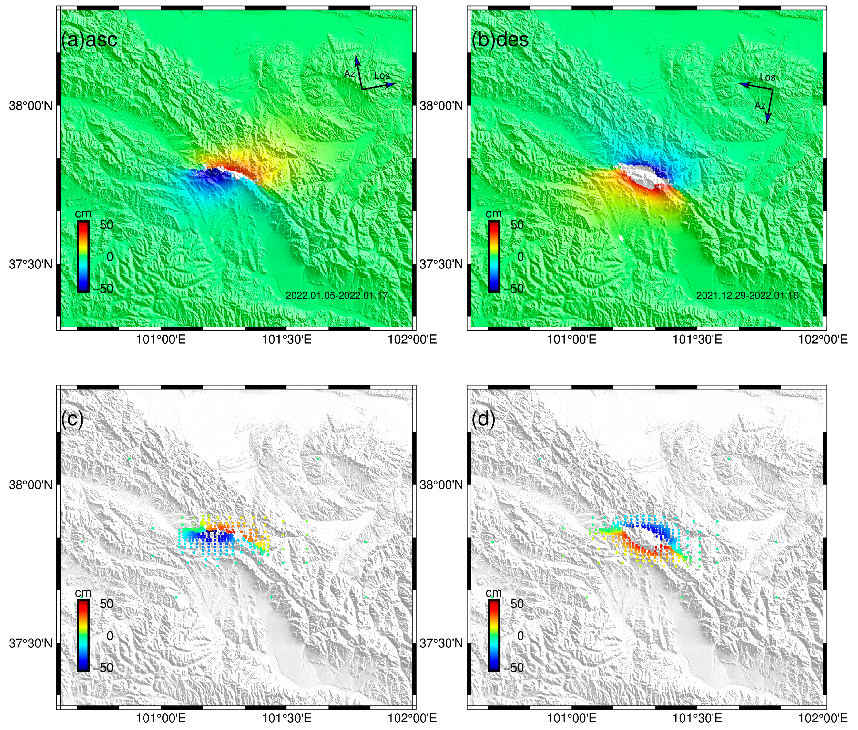
Xu et al. [40] provided the InSAR data used in this paper. Figure 9 shows the LOS shift of the InSAR ascending and descending orbits. This paper uses the ascending orbit T128 data from 5 January 2022 to 17 January 2022 and the descending orbit T33 data from 29 December 2021 to 10 January 2022 of the Sentinel-1 satellite. The variance-based quadtree sampling method is used to sample the ascending and descending orbit data. After sampling, the 334 points of the ascending orbit T128 are obtained, and 392 points of the descending orbit T33 are obtained, as shown in Figure 9. Using the LOS data and the wavelength of the Sentinel-1 satellite, the interferogram of the InSAR ascending and descending orbit is obtained via the modulus operation, as shown in Figure 10. Figure 10 shows that the observation data have serious decoherence in areas with large gate-source seismic deformation. The defect of observation data decorrelation further aggravates the situation in which the Markov chain of the MCMC algorithm touches the interval threshold under the conventional Bayesian framework.

Table 5. Inversion of initial model parameters of the source parameters of the Menyuan earthquake.

	Length/m	Width/m	Depth/m	Dip/°	Strike/°	X/m	Y/m	Strike-Slip/m	Dip–Slip/m
lower limit	2000	2000	0	50	80	−20,000	−20,000	−1	−1
upper limit	40,000	22,000	20,000	90	120	20,000	20,000	5	5
initial step size of MCMC	100	100	100	1	1	10	10	0.1	0.1
Random interval generation	15,152	11,708	13,006	75.68	96.87	/	/	3.49130	1.78740

Note: The actual step size is equal to the product of the initial step size and the random step size. Random interval generation means that in the upper and lower limit intervals, rand randomly generates a set of parameters to provide initial values for subsequent experiments to simulate the situation in which the initial values are unreliable. At this time, the upper and lower boundaries are limited only by random interval. The depth in this table is the bottom depth. The latitude and longitude start from the source location published by the USGS: Lon101.278, Lat37.815.

lists the initial model parameters of the inversion of the source parameters of the Menyuan earthquake. The initial values for longitude and latitude are based on the epicenter location published by the USGS, with a longitude of 101.278° and a latitude of 37.815°. These values are defined as the origin of the local planar coordinate system. In Table 5, X and Y represent the local planar coordinates of the source center derived from the inversion results. The final results can be converted to geodetic coordinates (longitude and latitude). The inverted source parameters are listed in

Table 6. One million sampling inversions of the source parameters of the Menyuan earthquake.

Scheme		Length/m	Width/m	Depth/m	Dip/°	Strike/°	X/m	Y/m	Strike-Slip/m	Dip-Slip/m
Random interval generation	optimum	17,008	10,878	13,263	89.49	107.87	669	−3708	4.18083	−0.09410
	mean	17,598	10,636	13,450	89.32	107.80	98	−3629	4.23621	−0.04755
	median	17,238	10,611	13,431	89.42	107.93	417	−3706	4.27682	−0.04661
	2.5%	17,030	10,460	13,281	88.93	107.02	−1520	−3733	3.97496	−0.08821
	97.5%	19,886	10,863	13,615	89.63	107.99	668	−3302	4.31517	−0.01307

Note: The best value refers to the maximum posterior probability solution. The total inversion time is 1 h, 59 min, and 4 s.

.

4.3. Results

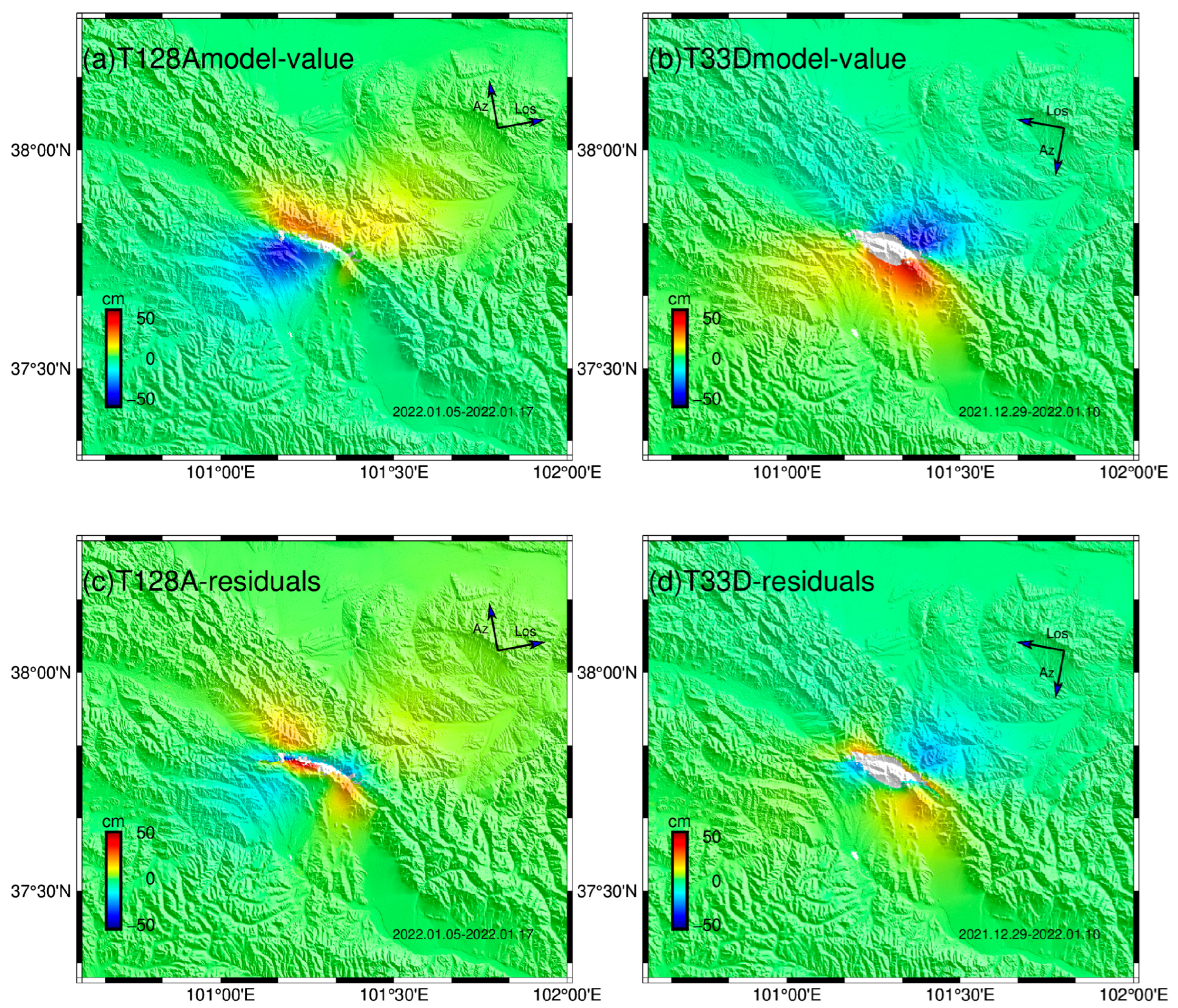
In this work, we employed the maximum a posteriori probability solution (i.e., the optimal value) and the 97.5% confidence interval values from the inversion results to forward-model the three-dimensional deformation values based on the original ascending and descending track InSAR data points. The LOS deformation values were calculated using Equations (7) and (8). These deformation values are consistent with the original observations (Figure 11 and Figure S9), with root mean square errors of 2.71 cm for the ascending track and 2.64 cm for the descending track using the maximum a posteriori probability solution, and 3.25 cm for the ascending track and 3.31 cm for the descending track using the 97.5% confidence interval values. The three-dimensional deformation results are shown in Figure 12 and Figure S10. The inversion results indicate that the Menyuan earthquake was primarily a strike-slip event dominated by strike-slip motion.

The seismic source parameters of the Menyuan earthquake in other related works in the literature are shown in

Table 7. Other literature source parameters of the Menyuan earthquake.

	East Longitude/°	North Latitude/°	Length/km	Depth/km	Strike/°	Dip/°	Slip/°
ingle-fault model in this paper	101.286	37.782	17	13.3	107.87	89.49	1.29
97.5%	101.286	37.785	19.9	13.6	107.99	89.63	0.17
CENC	101.26	37.77	/	10	/	/	/
GCMT	101.31	37.80	/	14.8	104/14	82/89	1/172
USGS	101.278	37.815	/	13.0	104/13	88/75	15/178
CEA-IGP Model 1	/	/	/	10	109/18	81/51	39/178
CEA-IGP Model 2	/	/	/	4	192/284	69/82	172/21
Xu et al. [40]	101.28	37.79	13.9	0.24	106.5	80.4	3.7
Li et al. [50]	/	/	8.8	/	104/109	80/80	0.5
Feng et al. [37]	101.17–101.41	37.73–37.81	3.1–17.9	/	88.65–127.2	70.88	/
Li et al. [43]	/	/	20.10	/	106.89	86.83	−5, −1
Yang et al. [53]	/	/	/	/	/	82	/

Note: CENC is the China Seismic Network, GCMT is the Global Moment Tensor, USGS is the US National Geological and Seismic Survey, and CEA-IGP refers to the Institute of Geophysics, China Earthquake Administration. Model 1 is the P-wave focal mechanism solution, and Model 2 is the seismic moment tensor inversion result. Li et al. [50], Feng et al. [37], and Li et al. [43] are multifault models. The depth of Xu et al. [40] is the midpoint depth of the upper boundary of the fault.

. Compared with those in other studies, the inverted results for the fault depth, strike angle, dip angle, and slip angle are overall closer to the results from the GCMT. This finding demonstrates the advantages and adaptability of the method used in this study for inverting complex seismic fault parameters.

5. Discussion

In this paper, to address the problem of the Bayesian MCMC algorithm, in which inappropriate interval settings and other reasons (for example, the upper and lower bounds of the interval do not include the correct value, the upper or lower bound is too close to the prior value or the correct value, or the prior value is too far from the correct value obtained from the inversion, etc.) cause Markov chains to fall into interval thresholds and affect the final inversion results, two interval determination strategies are proposed in the framework of the Bayesian algorithm, and the use of the root mean square error is proposed in the simulated earthquakes to measure the smooth distribution of the Markov chains.

We use simulated earthquakes to verify the effectiveness of the interval determination strategy. Twelve experimental schemes are set up, and the convergence plots of the Markov chain, with the root mean square error of its deviation from the true value during the inversion process, indicate that Strategy 1, ‘CFI’, effectively increases the convergence speed of the Markov chain. This allows it to reach a smooth distribution, even when the initial model parameters significantly deviate from the true values.

In contrast, Strategy 2, ‘IVI’, may not be suitable for Bayesian MCMC methods with large step lengths, likely because the initial model parameters in Scheme 11 deviate from the true values. In Bayesian MCMC algorithms in which the overall step length is normally distributed and small, compared with Strategy 1, Strategy 2 can better enhance the convergence speed and reduce the root mean square error.

After removing the first 200,000 nonconverted sampling points, Strategy 2 still has the smallest root mean square error among the twelve scenarios when the initial model is poor (Strategy 12). However, Strategy 2 consumes more computational resources and significantly decreases the inversion time due to the changing intervals with each sampling, as detailed in Table S1.

To verify the applicability of the interval determination strategy in real complex earthquakes, the source parameters of the Menyuan earthquake are inverted via the Bayesian MCMC algorithm under interval determination strategy 2 proposed in this paper. The inversion results reveal that the Menyuan earthquake was primarily a strike-slip event with a small amount of dip slip. Overall, the fault depth, strike angle, dip angle, and slip angle from the inversion results are closer to the GCMT results, revealing the advantages and adaptability of this method for inverting complex seismic fault parameters.

In addition, for other geophysical problems, within the Bayesian framework of geophysical inversion, as long as the input and output parameters include constraints on the upper and lower bounds of the interval and there are problems related to obtaining the upper and lower bounds, the interval strategy presented in this paper can be applied to these problems. This includes solid earth geophysical inversion issues such as lithofacies identification, magnetotelluric imaging, natural and microseismic monitoring, and fluid prediction.

6. Conclusions

Based on the experimental results, the conclusions of this study are summarized as follows:

(1)

When the range of seismic source parameters is unknown or ambiguous, Interval Determination Strategy 2 (IVI) should be adopted;

(2)

When an approximate range is known, Interval Determination Strategy 1 (CFI) is recommended;

(3)

When the interval is fully known and a reliable initial model can be obtained, the original interval constraint method should be used.

The proposed interval determination strategy based on the Bayesian MCMC algorithm demonstrates significant advantages in reliably estimating seismic source parameters. This method provides a novel solution for cases where parameter intervals are undefined (i.e., the upper and lower bounds set during inversion are unknown) and initial values are difficult to determine, offering considerable practical value.

Further research is needed to explore other Bayesian algorithms, such as variational Bayes—a Bayesian statistical method for approximate inference. Additionally, applying Bayesian algorithms to address complex multi-fault source mechanisms, similar to those observed in the Menyuan earthquake, represents an important research direction. Understanding the detailed structure of multi-fault focal mechanisms—including accurately resolving multi-fault geometries and analyzing seismic Coulomb stress accumulation [56]—is essential. These issues warrant further in-depth investigation.

References

1. Xu, C.; He, K. Advancements in Earthquake Cycle Deformation Research Based on Geodetic Observations. Geomat. Inf. Sci. Wuhan Univ. 2023, 48, 1736–1755. (In Chinese) [Google Scholar] [CrossRef]
2. Funning, G.J.; Fukahata, Y.; Yagi, Y.; Parsons, B. Method for the joint inversion of geodetic and seismic waveform data using ABIC: Application to the 1997 Manyi, Tibet, earthquake. Geophys. J. Int. 2014, 196, 1564–1579. [Google Scholar] [CrossRef]
3. Papadimitriou, E.; Karakostas, V.; Papazachos, C.; Foumelis, M.; Kiratzi, A.; Pikridas, C.; Bonatis, P.; Kostoglou, A.; Kourouklas, C.; Scordilis, E.; et al. The seismogenic structure of March 2021 Tyrnavos (central Greece) doublet (Mw6.3 and Mw6.0), constrained by aftershock locations and geodetic data. Geophys. J. Int. 2023, 235, 644–689. [Google Scholar] [CrossRef]
4. Wang, L.; Li, H. GBO algorithm for seismic source parameters inversion. Geod. Geodyn. 2023, 14, 182–190. [Google Scholar] [CrossRef]
5. Xi, C.; Wang, L.; Zhao, X.; Sun, Z.; Zhao, W.; Pang, M.; Wu, F. A simple weighting method for inverting earthquake source parameters using geodetic multisource data under Bayesian algorithm. Geophys. J. Int. 2024, 237, 1142–1156. [Google Scholar] [CrossRef]
6. Okada, Y. Internal deformation due to shear and tensile faults in a half-space. Bull. Seismol. Soc. Am. 1992, 82, 1018–1040. [Google Scholar] [CrossRef]
7. Picozzi, M.; Oth, A.; Parolai, S.; Bindi, D.; De Landro, G.; Amoroso, O. Accurate estimation of seismic source parameters of induced seismicity by a combined approach of generalized inversion and genetic algorithm: Application to The Geysers geothermal area, California. J. Geophys. Res. Solid Earth 2017, 122, 3916–3933. [Google Scholar] [CrossRef]
8. Yang, Y.; Chen, Q.; Xu, Q.; Liu, G.; Hu, J. Source model and Coulomb stress change of the 2015 Mw 7.8 Gorkha earthquake determined from improved inversion of geodetic surface deformation observations. J. Geod. 2019, 93, 333–351. [Google Scholar] [CrossRef]
9. Zhao, Y.; Xu, C. Adaptive multi-start Gauss-Newton approach for geodetic data inversion of earthquake source parameters. J. Geod. 2020, 94, 17. [Google Scholar] [CrossRef]
10. Wang, L.; Xu, R.; Yu, F. Genetic Nelder-Mead neural network algorithm for fault parameter inversion using GPS data. Geod. Geodyn. 2022, 13, 386–398. [Google Scholar] [CrossRef]
11. Xu, C.; Zheng, G.; Niu, J. Recent developments in seismological geodesy. Geod. Geodyn. 2016, 7, 157–164. [Google Scholar] [CrossRef]
12. Simutė, S.; Boehm, C.; Krischer, L.; Gokhberg, A.; Vallée, M.; Fichtner, A. Bayesian Seismic Source Inversion With a 3-D Earth Model of the Japanese Islands. J. Geophys. Res. Solid Earth 2023, 128, e2022JB024231. [Google Scholar] [CrossRef]
13. Wei, G.; Chen, K.; Meng, H. Bayesian Inversion of Finite-Fault Earthquake Slip Model Using Geodetic Data, Solving for Non-Planar Fault Geometry, Variable Slip, and Data Weighting. J. Geophys. Res. Solid Earth 2023, 128, e2022JB025225. [Google Scholar] [CrossRef]
14. Amey, R.M.J.; Hooper, A.; Morishita, Y. Going to any lengths: Solving for fault size and fractal slip for the 2016, Mw6.2 Central Tottori earthquake, Japan, using a transdimensional inversion scheme. J. Geophys. Res. Solid Earth 2019, 124, 4001–4016. [Google Scholar] [CrossRef]
15. Amey, R.M.J.; Hooper, A.; Walters, R.J. A Bayesian method for incorporating self-similarity into earthquake slip inversions. J. Geophys. Res. Solid Earth 2018, 123, 6052–6071. [Google Scholar] [CrossRef]
16. Bagnardi, M.; Hooper, A. Inversion of surface deformation data for rapid estimates of source parameters and uncertainties: A Bayesian approach. Geochem. Geophys. Geosystems 2018, 19, 2194–2211. [Google Scholar] [CrossRef]
17. Izzatullah, M.; Van Leeuwen, T.; Peter, D. Bayesian seismic inversion: A fast sampling Langevin dynamics Markov chain Monte Carlo method. Geophys. J. Int. 2021, 227, 1523–1553. [Google Scholar] [CrossRef]
18. Zhang, C.; Chen, T. Bayesian slip inversion with automatic differentiation variational inference. Geophys. J. Int. 2022, 229, 546–565. [Google Scholar] [CrossRef]
19. Zhao, X.; Curtis, A.; Zhang, X. Bayesian seismic tomography using normalizing flows. Geophys. J. Int. 2022, 228, 213–239. [Google Scholar] [CrossRef]
20. Wang, L.; Sun, L.; Xu, G. An Improved Bayesian von Karman Regularization Method for the Joint Inversion of GNSS and InSAR Data. J. Surv. Eng. 2023, 149, 04022016. [Google Scholar] [CrossRef]
21. Sun, L.; Wang, L.; Xu, G.; Wu, Q. A new method of variational Bayesian slip distribution inversion. J. Geod. 2023, 97, 10. [Google Scholar] [CrossRef]
22. Wang, L.; Xi, C. An improved MCMC algorithm for inversion of source parameters using GPS data under Bayesian framework. Chin. J. Geophys. 2024, 67, 3367–3385. (In Chinese) [Google Scholar] [CrossRef]
23. Pedersen, R.; Jónsson, S.; Árnadóttir, T.; Sigmundsson, F.; Feigl, K. Fault slip distribution of two June 2000 Mw6.5 earthquakes in South Iceland estimated from joint inversion of InSAR and GPS measurements. Earth Planet. Sci. Lett. 2003, 213, 487–502. [Google Scholar] [CrossRef]
24. Wright, T.J.; Lu, Z.; Wicks, C. Source model for the Mw6.7, 23 October 2002, Nenana mountain earthquake (Alaska) from InSAR. Geophys. Res. Lett. 2003, 30, 18. [Google Scholar] [CrossRef]
25. Wang, L.; Gao, H.; Feng, G.; Xu, W. Source parameters and triggering links of the earthquake sequence in central Italy from 2009 to 2016 analyzed with GPS and InSAR data. Tectonophysics 2018, 744, 285–295. [Google Scholar] [CrossRef]
26. Wang, L.; Xu, R. Multistart Nelder–Mead neural network algorithm for earthquake source parameter inversion of 2017 Bodrum–Kos earthquake. J. Surv. Eng. 2021, 147, 04021014. [Google Scholar] [CrossRef]
27. Tarantola, A. Inverse Problem Theory and Methods for Model Parameter Estimation; Elsevier: Amsterdam, The Netherlands, 1987. [Google Scholar]
28. Chai, H.; Chen, K.; Wei, G.; Fang, R.; Zou, R.; Zhu, H. Coseismic Deformation Monitoring Using BDS-3 and Ultra-High Rate GNSS: A Case Study of the 2021 Maduo Mw7.4 Earthquake. Geomat. Inf. Sci. Wuhan Univ. 2022, 47, 946–954. (In Chinese) [Google Scholar] [CrossRef]
29. Xiong, W.; Chen, W.; Wang, D.; Wen, Y.; Nie, Z.; Liu, G.; Dijin, W.; Yu, P.; Qiao, X.; Zhao, B. Coseismic slip and early afterslip of the 2021 Mw7.4 Maduo, China earthquake constrained by GPS and InSAR data. Tectonophysics 2022, 840, 229558. [Google Scholar] [CrossRef]
30. Jiang, W.; Xu, C.; Li, Z.; Wu, Y.; Tan, K.; Geng, J.; Chun, Y.; Zheng, G.; Wen, Y.; He, K.; et al. Using space observation techniques to study temporal and spatial characteristics of seismogenic process, occurrence and deformation of the Qinghai Madoi Mw7.4 earthquake. Chin. J. Geophys. 2022, 65, 495–508. (In Chinese) [Google Scholar] [CrossRef]
31. Fabris, M.; Battaglia, M.; Chen, X.; Menin, A.; Monego, M.; Floris, M. An integrated InSAR and GNSS approach to monitor land subsidence in the Po River Delta (Italy). Remote Sens. 2022, 14, 5578. [Google Scholar] [CrossRef]
32. Lazos, I.; Papanikolaou, I.; Sboras, S.; Foumelis, M.; Pikridas, C. Geodetic Upper Crust Deformation Based on Primary GNSS and INSAR Data in the Strymon Basin, Northern Greece—Correlation with Active Faults. Appl. Sci. 2022, 12, 9391. [Google Scholar] [CrossRef]
33. Shen, G.; Fu, W.; Guo, H.; Liao, J. Water body mapping using long time series Sentinel-1 SAR data in Poyang Lake. Water 2022, 14, 1902. [Google Scholar] [CrossRef]
34. Brouwer, W.S.; Hanssen, R.F. A treatise on InSAR geometry and 3D displacement estimation. IEEE Trans. Geosci. Remote Sens. 2023, 61, 1–11. [Google Scholar] [CrossRef]
35. Hu, J.; Ding, X.; Zhang, L.; Sun, Q.; Li, Z.; Zhu, J.; Lu, Z. Estimation of 3-D surface displacement based on InSAR and deformation modeling. IEEE Trans. Geosci. Remote Sens. 2016, 55, 2007–2016. [Google Scholar] [CrossRef]
36. Peltier, A.; Froger, J.L.; Villeneuve, N.; Catry, T. Assessing the reliability and consistency of InSAR and GNSS data for retrieving 3D-displacement rapid changes, the example of the 2015 Piton de la Fournaise eruptions. J. Volcanol. Geotherm. Res. 2017, 344, 106–120. [Google Scholar] [CrossRef]
37. Feng, W.; Li, Z. PSO hybrid algorithm inversion strategy of source parameters under InSAR data constraints. Prog. Geophys. 2010, 25, 1189–1196. (In Chinese) [Google Scholar] [CrossRef]
38. Wang, L.; Gao, H.; Feng, G. InSAR and GPS data were used to analyze the triggering relationship and stress influence of two Mw>6 earthquakes in southwestern Taiwan. Acta Geod. Et Cartogr. Sin. 2019, 60, 2578–2588. (In Chinese) [Google Scholar] [CrossRef]
39. Lohman, R.B.; Simons, M. Some thoughts on the use of InSAR data to constrain models of surface deformation: Noise structure and data downsampling. Geochem. Geophys. Geosyst. 2005, 6, 2004GC000841. [Google Scholar] [CrossRef]
40. Xu, G.; Xu, X.; Yi, Y.; Wen, Y.; Wang, Q.; Li, K.; Ren, J. Seismogenic structure of the 2022 Menyuan Mw6.6 earthquake, Qinghai Province, constrained by InSAR and Gaofen-7 observation. Chin. J. Geophys. 2022, 65, 4704–4724. (In Chinese) [Google Scholar] [CrossRef]
41. He, L.; Feng, G.; Wang, Y.; Xiong, Z.; Gao, H.; Liu, X. Geodetic source models of the 2016–2022 Menyuan Earthquake sequence (Northeastern Tibet) inferred from InSAR and optical observations. Geophys. J. Int. 2024, 236, 470–479. [Google Scholar] [CrossRef]
42. Li, K.; Tapponnier, P.; Xu, X.; Kang, W. The 2022 Ms 6.9 Menyuan earthquake: Surface rupture, Paleozoic suture re-activation, slip-rate and seismic gap along the Haiyuan fault system, NE Tibet. Earth Planet. Sci. Lett. 2023, 622, 118412. [Google Scholar] [CrossRef]
43. Li, Y.; Jiang, W.; Li, Y.; Shen, W.; He, Z.; Li, B.; Li, Q.; Jiao, Q.; Tian, Y. Coseismic rupture model and tectonic implications of the January 7, 2022, Menyuan Mw6.6 earthquake constraints from InSAR observations and field investigation. Remote Sens. 2022, 14, 2111. [Google Scholar] [CrossRef]
44. Wang, J.; Ding, L.; He, J.; Cai, F.; Wang, C.; Zhang, Z. Research of seismogenic structures of the 2016 and 2022 Menyuan earthquakes, in the Northeastern Tibetan plateau. Remote Sens. 2023, 15, 742. [Google Scholar] [CrossRef]
45. Yu, C.; Li, Z.; Song, C.; Han, B.; Chen, B.; Li, X.; Peng, J. Fault structure and slip mechanics of the 2022 Mw6.7 Menyuan earthquake revealed by coseismic rupture observations. Tectonophysics 2024, 872, 230192. [Google Scholar] [CrossRef]
46. Zhang, Y.; Chen, J.; Gong, W.; Han, N.; Liu, Y.; Shan, X. Geodetic modeling of the 2022 Mw6.6 Menyuan earthquake: Insight into the strain-partitioned northern Qilian Shan fault system and implications for regional tectonics and seismic hazards. Geophys. J. Int. 2023, 233, 1987–2003. [Google Scholar] [CrossRef]
47. Zuo, K.; Luo, J.; Zhao, C.; Chen, J.; Yin, X. Spatiotemporal distribution characteristics of seismicity and seismogenic environment in the Menyuan area, Qinghai Province. Chin. J. Geophys. 2023, 66, 1460–1480. (In Chinese) [Google Scholar] [CrossRef]
48. Xu, X.; Wu, X.; Yu, G.; Li, K. Seismo-geological signatures for identifying M≥7.0 earthquake risk areas and their preliminary application in mainland China. Seismol. Geol. 2017, 39, 219–275. (In Chinese) [Google Scholar] [CrossRef]
49. Lü, M.; Chen, K.; Chai, H.; Geng, J.; Zhang, S.; Fang, L. Joint inversion of InSAR and high-rate GNSS displacement waveforms for the rupture process of the 2022 Qinghai Menyuan M6.9 earthquake. Chin. J. Geophys. 2022, 65, 4725–4738. (In Chinese) [Google Scholar] [CrossRef]
50. Li, Z.; Han, B.; Liu, Z.; Zhang, M.; Yu, C.; Chen, B.; Liu, H.; Du, J.; Zhang, S.; Zhu, W.; et al. Source Parameters and Slip Distributions of the 2016 and 2022 Menyuan, Qinghai Earthquakes Constrained by InSAR Observations. Geomat. Inf. Sci. Wuhan Univ. 2022, 47, 887–897. (In Chinese) [Google Scholar] [CrossRef]
51. Feng, W.; He, X.; Zhang, Y.; Fang, L. Seismic faults of the 2022 Mw6.6 Menyuan, Qinghai earthquake and their implication for the regional seismogenic structures. Chin. Sci. Bull. 2023, 68, 254–270. (In Chinese) [Google Scholar] [CrossRef]
52. Wan, Y.; Huang, S.; Wang, F.; Xu, Y.; Yu, H. Fault geometry and slip characteristics revealed by the 2022 Menyuan earthquake sequence. Chin. J. Geophys. 2023, 66, 2796–2810. (In Chinese) [Google Scholar] [CrossRef]
53. Yang, H.; Wang, D.; Guo, R.; Xie, M.; Zang, Y.; Wang, Y.; Yao, Q.; Cheng, C.; An, Y.; Zhang, Y. Rapid report of the 8 January 2022 MS6.9 Menyuan earthquake, Qinghai, China. Earthq. Res. Adv. 2022, 2, 100113. [Google Scholar] [CrossRef]
54. Xu, S. Co-seismic deformation filed and fault-slip distribution of the Menyuan Ms6.9 earthquake on January 8, 2022, constrained by GNSS observations. J. Earthq. Eng. 2023, 45, 401–409. (In Chinese) [Google Scholar] [CrossRef]
55. Deng, Q. Active tectonics and earthquake activities in China. Earth Sci. Front. 2003, 10 (Suppl. S1), 66–73. (In Chinese) [Google Scholar]
56. Maurer, J.; Johnson, K.; Wallace, L.; Hamling, I.; Williams, C.; Rollins, C.; Gerstenberger, M.; Van Dissen, R. Geodetic strain rates for the 2022 update of the New Zealand National Seismic Hazard Model. Bull. Seismol. Soc. Am. 2023, 114, 57–77. [Google Scholar] [CrossRef]
Figure 1. Markov chain case of touching the threshold (a case of erroneous convergence caused by interval constraints in synthetic experiments).
Remotesensing 17 03151 g001
Figure 2. Flowchart of the MCMC process for solving the Bayesian posterior probability density function.
Remotesensing 17 03151 g002
Figure 3. Three-dimensional deformation field of the simulated seismic GNSS data.
Remotesensing 17 03151 g003
Figure 4. InSAR data of simulated earthquakes (in order, the three-direction deformation field and LOS displacement field without error; the three-direction deformation field and LOS displacement field with error are applied; interference phase diagram and quadtree down sampling).
Remotesensing 17 03151 g004
Figure 5. First 20,000 Markov chain sampling plots of the twelve schemes.
Remotesensing 17 03151 g005
Figure 6. Posterior probability distribution plots for all the Markov chain parameters of the twelve schemes: (a) length, (b) width, and (c) depth. Among them, (df) represent the locally amplified posterior probability density functions in their respective subfigures.
Remotesensing 17 03151 g006
Figure 7. Posterior probability distribution plots for all Markov chain parameters of the twelve schemes: (a) dip angle, (b) strike angle, (c) dip-slip component, and (d) strike-slip component. Among them, (eh) represent the locally amplified posterior probability density functions in their respective subfigures.
Remotesensing 17 03151 g007
Figure 8. Source map of the Menyuan earthquake (the active faults in and around the Menyuan earthquake are indicated by the red-brown line segments, with data from Deng. [55]). The yellow triangles represent the GPS stations near the Menyuan area, and the GPS station data are from Xu [54]. The red pentagram in the figure represents the epicenter location of the 2022 Menyuan earthquake provided by USGS, the blue pentagram represents the epicenter location of the 2022 Menyuan earthquake provided by GCMT, and the green and purple pentagrams denote the epicenter locations of historical earthquakes mentioned in the text. The color of the focal mechanism beads represents the depth.
Remotesensing 17 03151 g008
Figure 9. InSAR data of the Menyuan earthquake deformation field: (a) T128 lift, (b) T33 descending orbit, (c) deformation point of the ascending data T128 quadtree after downsampling, and (d) deformation point of the deorbital data T33 after quadtree downsampling.
Remotesensing 17 03151 g009
Figure 10. Interferogram of Menyuan earthquake InSAR data ((a) T128 lift and (b) T33 descent orbit. The LOS deformation value is converted by the modulus operation).
Remotesensing 17 03151 g010
Figure 11. Maximum a posteriori probability model value forward map ((a) the forward value of the T128 ascending rail model parameters, (b) the forward value of the T33 descending orbit model parameters, (c) the residual error between the forward value and the observed value of the parameters of the T128 lift model, and (d) residual between the forward value and the observed value of the parameters of the T33 descending orbit model).
Remotesensing 17 03151 g011
Figure 12. Three-direction deformation map of the forward model of the maximum posterior probability model value. (In Figure 12, subgraphs (a), (b), and (c) are the three-direction deformation values of the forward ascending orbit in turn, which are the east-west direction, north-south direction, and vertical direction, respectively; subgraphs (d), (e), and (f) are the three-direction deformation values of the descending orbit, which are the east-west, north-south, and vertical directions, respectively).
Remotesensing 17 03151 g012