Abstract
As one of the world’s leading grain producers, Brazil stands out in soybean and corn production. Accurate estimation of key crop phenological stages is essential for agricultural decision-making, especially considering Brazil’s vast territory, climatic diversity, and increasing frequency of extreme weather events. This study investigated the applicability of the NDVI, EVI, WDRVI, and NDWI, derived from Harmonized Landsat Sentinel-2, to identify crop sowing and harvest dates at the field scale. We extracted the vegetative peak from each vegetation index time series and identified the left and right inflection points around the peak to delineate the crop season. A double-logistic function and a derivative approach were applied to identify the Start of Season, Peak of Season, and End of Season. For both soybeans and corn, the RMSE ranged from 5 to 8 days for sowing dates, while for harvest dates it ranged from 6 to 15 days for corn. Despite these differences, all vegetation indices exhibited robust performance, with Spearman correlation values between 0.56 and 0.84. Our findings indicate that the use of different indices does not have a significant impact on the results, as long as the adjustment of temporal parameters for the phenological metrics is appropriate for each index.
1. Introduction
Significant phenological heterogeneity is observed in annual crops when evaluated concurrently, due to the interplay between wide-ranging variables that farmers consider in their day-to-day management of different crop production undertakings [1]. These variables include cultivated species, type of cultivar, sowing and harvest periods, soil type, climatic conditions and many others. The accurate detection and prediction of the phenological stage is mainly driven by the accumulated growing degree days and photoperiod (number of daylight hours) but are also affected by other environmental factors [2] and vary among cultivars [3]. In studies of crop phenology, sowing and harvest dates are the most critical temporal markers to monitor due to their impact on the supply chain [4].
Planting dates significantly impact crop development, as they determine the initial interaction with the prevailing weather conditions. Consequently, these dates are also closely related to yield, which is shaped by environmental conditions throughout the growing season. While farmers can manage factors like crop variety and fertilizer needs, climate variables change independently of the farmer’s will [5]. Conversely, the harvest date holds significant relevance for the entire agricultural supply chain, encompassing production, processing, logistics, storage, and marketing [6]. For instance, in Brazil, early soybean planting increases drought risk and the potential need for replanting. Closely related to this is the late sowing of soybeans, which can affect the second-crop corn, by shortening the optimal sowing window, reducing the available precipitation for the corn development and/or increasing the risk of frost events [7].
Conventionally, data regarding crop phenology are obtained through farm surveys, which involve direct observation and recording of phenological events at the field level rather than solely relying on interviews with farmers. While farmer interviews may supplement specific information, such as sowing and harvest dates, most detailed phenological data require systematic field assessments conducted by researchers. Although this field-level knowledge is of paramount agronomic importance, the availability of comprehensive datasets containing such information to the public remains limited, not only in developing countries but also in their developed counterparts [8]. This limitation arises because most farmers do not systematically record these data, making researchers’ field surveys essential yet infrequent and resource-intensive.
Furthermore, when accessible, most crop phenological information is of little use to the farmer because it is aggregated at the national or regional scales [6,9,10]. In contrast, field-scale records, when available, are often limited to small areas and specific periods, such as a single agricultural season [11].
The generation of field-scale statistics can significantly improve our understanding in various research fields, such as the analysis of yield gaps [12] and assessing the impact of agriculture in response to climate change. A comprehensive database containing this type of information could help identify areas where substantial yield increases could be achieved by adjusting sowing dates [13]. This goal could be achieved through specific public policies, such as the improvement of the Agricultural Climate Risk Zoning (ZARC) in Brazil [14].
To address this limitation, Remote Sensing (RS) datasets at diverse spatial and temporal resolutions, have been employed to map crop phenology at the field level [8,11,13,15,16,17,18]. Among these are Sentinel and Landsat satellite data, which have immense potential to aid with phenology, when their medium-resolution observations are used to inferentially obtain crucial information about the crop development cycle [19,20,21].
Sentinel-2 is a constellation consisting of two satellites, Sentinel-2A and Sentinel-2B, which provide optical imagery from the MultiSpectral Instrument (MSI) at spatial resolutions ranging from 10 to 60 m and a revisit period of 5 days [22]. Landsat-8, launched on 11 February 2013 [23], and its successor, Landsat-9, launched on 27 September 2021 [24], are both equipped with the Operational Land Imager (OLI) sensor. The OLI sensor comprises nine spectral bands, six of which are specifically designed for terrestrial applications at a spatial resolution of 30 m [25].
Despite this, broad-based estimation of agricultural crop phenology with medium spatial resolution data from single optical sensors like MSI and OLI remains challenging due to their insufficient acquisition frequency for accurate estimations [26]. To address this, the Harmonized Landsat Sentinel-2 (HLS) product represents a significant advancement, leveraging data harmonization techniques to combine MSI and OLI sensor data. This harmonization has significantly increased temporal resolution to approximately a 2-day revisit period, while maintaining the 30 m spatial resolution designed for terrestrial applications [27]. Consequently, HLS offers a promising solution to overcome this limitation and has shown significant potential in phenological studies [28,29,30].
Building on this advancement, phenological stages can be estimated by extracting metrics from Vegetation Index Time Series (VITS). Derived from spectral bands sensitive to various crop characteristics [31], these indices correlate with typical vegetation development stages. While various indices can be used for this purpose, the Normalized Difference Vegetation Index (NDVI) [32], Enhanced Vegetation Index (EVI) [33], Wide Dynamic Range Vegetation Index (WDRVI) [34], and Normalized Difference Water Index (NDWI) [35] are among the most commonly employed in crop phenological studies [31]. Crop phenology detection using VITS, in turn, can be broadly divided into three main methodological categories: empirical methods, phenological-matching methods, and simulation-based methods [31,36].
Phenological-matching methods incorporate ancillary data to support and refine phenological detection. A typical example is the two-step filtering method [37], which uses a reference VI series constructed from ground-truth observations (shape model) and fits the target pixel’s time series to this reference using geometric alignment. The challenge of directly matching phenological metrics derived from VITS to field-observed dates (such as sowing and harvest) is widely recognized in the literature. Methods such as Shape Model Fitting [38,39] and its Spatiotemporal Variants [40] have been proposed to improve robustness by fitting generic curves to the VI data. On the other hand, simulation-based methods employ mechanistic models to simulate phenological development. These models are often based on physical principles and consider environmental factors [31].
Empirical methods rely exclusively on the VITS data from the target pixel and do not incorporate external auxiliary information. This category includes both threshold-based and inflection-point-based approaches. Threshold-based methods assume that a specific phenological stage occurs when the vegetation index reaches a certain percentage of the seasonal dynamic range (relative threshold) or a fixed VI value (absolute threshold) [15,18,41,42,43,44]. Although these methods are straightforward to implement, threshold definitions can vary significantly between regions and must be adapted to local environmental conditions, which hinders their broader applicability. Furthermore, the type of crop exhibits different phenological behaviors, requiring specific adjustments to the adopted parameters. The crop cycle can also influence the timing of phenological events and, consequently, the definition of appropriate thresholds for each case [45].
However, despite the increasing availability of high-resolution satellite data and various vegetation indices, a significant knowledge gap remains about which vegetation index is most suitable for accurately estimating sowing and harvest dates for key crops such as soybean and corn. While the general applications of vegetation indices are well documented, the comparative effectiveness of these different indices in capturing the nuances of crop phenology under diverse field conditions remains largely unexplored. Furthermore, although empirical methods are widely used due to their simplicity, they exhibit limitations related to the variability of results when applied across different contexts (regions, crops, and growing cycles), highlighting the need for methodological improvements to enhance their robustness and reduce this sensitivity.
Moreover, achieving accurate field-scale estimates often necessitates precise adjustments for temporal parameters, and the impact of these fine-tuned adjustments on the performance of different vegetation indices for specific crops is not yet fully understood or optimized. Understanding these index-specific performances and their necessary temporal adjustments is paramount for developing robust, practical tools for agricultural decision-making and yield forecasting at the resolution needed by farmers and agricultural planners.
Therefore, this study aims to fill this critical gap by comparatively investigating the applicability and performance of NDVI, EVI, WDRVI, and NDWI, derived from HLS data, for reliably determining field-scale sowing and harvest dates for corn and soybeans in Brazil’s Central-West and South regions. Our approach specifically explores the impact and necessity of fine-tuning temporal parameters for each vegetation index to achieve optimal accuracy, thereby advancing the methodology for precise phenological monitoring in complex agricultural systems.
2. Materials and Methods
2.1. Study Areas
Our approach for estimating sowing and harvest dates was tested using soybean and corn field data in two Brazilian states: Paraná (PR) and Mato Grosso (MT) (Figure 1). Located in the Central-West region, MT state encompasses three biomes: the Amazon biome, covering 511,912 km2 (59.9%); the Cerrado biome (Brazilian Savanna), with 337,736 km2 (39.5%); and the Pantanal biome, with 5352 km2 (0.6%). In PR state, located in the south region, the Atlantic Forest biome predominates, covering 196,146 km2 (98.4%), with some areas of Cerrado biome, covering 3124 km2 (1.6%) [46]. Figure 1 shows the geographic locations of agricultural areas and validation crop fields in PR and MT that were targeted in this investigation.
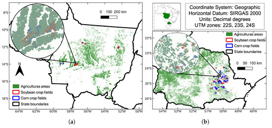
Figure 1.
Geographic locations of agricultural areas and validation crop fields in Brazil’s PR and MT that were targeted in this investigation: (a) Mato Grosso, Brazil. (b) Paraná, Brazil.
In these study areas, soybean and corn are mostly cultivated through rainfed double-cropping. Thus, the sowing period depends on the onset of the rainy season [47]. Soybean sowing typically begins between late winter and early spring, coinciding with increased rainfall. However, climatic differences are observed between regions: PR experiences a wet and cold winter, whereas MT has a hot and dry winter, precluding rainfed soybean cultivation during this period [48]. Furthermore, both states enforce a mandatory window period of 60 to 90 days, during which soybean cultivation is prohibited to mitigate pest pressure, particularly soybean rust [49]. Soybean harvesting generally takes place during the rainy summer in both states, usually in January and February. Subsequently, second-crop corn is often sown immediately after soybean harvesting, sometimes even on the same day [48], with the harvesting of second-crop corn extending from July to September.
2.2. Roadmap
We accessed HLS data for crop fields from NASA’s Earthdata database [50] and processed them by applying linear interpolation and noise removal. Using crop calendars, we first estimated the vegetative period and extracted the vegetative peak from each VITS. This was followed by identifying the left and right inflection points, which were identified as minima within specified windows, with the minimum value being rounded upwards to better match the crop growth curve. All values preceding or following these points were adjusted to their respective inflection values, and a double-logistic function [51] was fitted to the series. From the resulting curve, we extracted the Start of Season (SOS), Peak of Season (POS), and the End of Season (EOS), with SOS and EOS defined as 10% and 90% of the distance between respective inflection points and the POS [52]. Finally, results were analyzed and validated. The roadmap for this process is shown in Supplementary Materials in Figure S1—A roadmap of the stages of crop phenology derived from HLS time series.
2.3. Reference Data
We utilized a dataset provided by SLC Agricola S.A. (https://www.slcagricola.com.br/en/) in MT. SLC operates eight farms and offers a comprehensive database containing crop field geometries and precise information on sowing and harvest dates for 588 soybean crop fields, comprising 290 during the 2019/2020 growing season and 298 during the 2020/2021 growing season. Additionally, SLC Agricola supplied details on 442 corn second-crop crop fields, comprising 125 during the 2019/2020 growing season, 145 during the 2020/2021 growing season, and 172 during the 2020/2021 growing season. In PR, the ABC Foundation (https://fundacaoabc.org/) supplied reliable ground truth data, enabling the analysis of 1093 fields from the 2019/2020 growing season for soybeans and 461 fields from the 2021/2022 growing season for first-crop corn (Figure 1).
2.4. Image Time Series Processing
We used version 2.0 HLS data [27,53] from NASA’s Earthdata database [50], which provides the Sentinel-2 HLSS30.002 [54] and Landsat-8/9 HLSL30.002 [55] data products we needed. HLS is a virtual constellation (VC) of surface reflectance data generated from Level-1 products of Landsat 8/OLI (L1T) and Sentinel-2/MSI (L1C). The generation of this data is based on a set of algorithms that enable the integration of data from the OLI and MSI sensors through atmospheric correction, cloud and cloud-shadow masking, spatial co-registration, common gridding, Bidirectional Reflectance Distribution Function (BRDF) normalization, and spectral bandpass adjustment to produce seamless and harmonized products [27].
We utilized HLS imagery covering approximately 30 days before sowing and 30 days after harvest to ensure that the entire crop cycle was covered in the period between late August 2019 and late September 2020. On average, 40 images per field were obtained, providing a mean temporal resolution of 4–5 days after cloud-contaminated images were removed.
Cloud masking in HLS images was performed using an adaptation of the Fmask 4.0 algorithm, originally developed for Sentinel-2 (S10) and Landsat (S30) products [56]. Fmask is a well-established cloud detection algorithm also utilized with Sentinel-2 [57]. It is used to identify potential cloud pixels through spectral tests, after which the identified pixels are then combined with provisional cloud shadow pixels using sensor geometry, a Digital Elevation Model (DEM), and an iterative altitude search. This image cleaning process was necessary because cloud cover and shadows are some of the major sources of noise in optical satellite data that need to be reduced [56,57]. Using the cloud-masked HLS imagery, we derived NDVI following the standard formulation; the computation steps and the rationale for this choice are described below.
We used four different band wavelengths (BLUE: 0.45–0.51 μm; RED: 0.64–0.67 μm; NIR: 0.78–0.88 μm, SWIR: 1.57–1.65 μm) to calculate four different VITS. Although the NDVI is highly sensitive to scattering and atmospheric absorption [58] because it is derived from two spectral bands only [32], it can still aid in the monitoring of large-scale cropland [59] due to its high sensitivity to canopy background brightness conditions [60]. The calculation of NDVI aims to eliminate seasonal differences in solar elevation angle and minimize the effects of atmospheric attenuation in multitemporal imagery [61]. This index is widely used in crop monitoring because of its sensitivity to the presence of chlorophyll and other plant pigments that are responsible for absorbing photosynthetically active radiation [60], which is directly related to the production of plant biomass.
However, a key limitation of this index is the occurrence of asymptotic saturation, which results in a low sensitivity for detecting variations in increasing plant biomass beyond a certain developmental stage, typically under conditions of high leaf area index [62,63,64,65]. When using data from the RED band (region of high chlorophyll absorption) and the NIR band (region with a reflectance plateau from vegetation canopies), errors in biomass estimation may occur [66]. This limitation compromises its usefulness in the estimation of agricultural phenology, given that changes in biomass can be a factor correlated with crop growth stages.
The identification of NDVI saturation in previous studies, both for corn and soybean, has led to the exploration of other indices, such as EVI [33], which is less likely to saturate due to its enhanced sensitivity to variations in canopy structure, plant physiognomy, canopy architecture, and high biomass levels [58,67]. In general, EVI values are lower than those of NDVI for the same vegetation because of the virtual absence of saturation [68].
Having recognized NDVI’s saturation limitations, researchers attempted to improve its sensitivity to moderate and high-density biomass by offering the WDRVI [34] and showed a linear relationship with the leaf area index of corn and soybeans [69]. The only way to broaden the NDVI dynamic range is to rely on an unsaturated NIR band under high biomass conditions. NDVI sensitivity to NIR reflectance can be increased by introducing a coefficient that increases reflectance in the NIR band, thereby reducing the disparity between the contributions of the NIR and RED bands in the determination of the NDVI value [34]. Because WDRVI can be negative for low-to-moderate vegetation density, we decided to calculate it at following the recommendations in [70].
Further enhancing crop monitoring in areas where vegetation exhibits high water content has important agricultural applications; therefore, the NDWI [35] was proposed because it is sensitive to the liquid water content in vegetation. This index utilizes two bands located in the NIR and SWIR 860 and 1240 nm wavelengths, respectively. Since both bands are in the infrared region, their responses are expected to be similar. Because the absorption of radiation by liquid water at 860 nm is negligible and at 1240 nm is weak, NDWI becomes sensitive to changes in the liquid water content in the vegetation canopy [35]. This index is a reliable metric in the monitoring of phenology because the water content in vegetation changes during different stages of crop growth [71].
2.5. Extraction of Phenological Metrics
Beyond atmospheric noise are the VITS patterns of soybeans and corn, which are similar to those of off-season vegetation (e.g., weeds, cover crops) during periods before sowing and after harvest. Although our study focused on predefined agricultural areas with a bimodal growing season for soybean and corn, the presence of off-season vegetation before the main crop sowing could interfere with the remote sensing-based identification of the crop’s growth start [72]. To minimize this influence in our VITS, preprocessing included filtering the target crops by their seasonality. This segregation involved (1) the use of a window period to identify inflection points [9] and (2) the application of the double-logistic function [51] to smooth the VITS by fitting a smoothing curve to the HLS data observations.
In fitting the double-logistic model to VITS, the algorithm automatically estimated the initial parameters, optimizing them according to the observed dynamics of each crop. In this estimation, parameter p0 was calculated as the mean of the minimum values of the analyzed variable before and after the vegetative peak, thereby representing the basal level of the series. Parameter p1 corresponds to the maximum value recorded throughout the time series, capturing the phase of greatest vegetative vigor. The growth and decline rates, represented by p2 and p4, were determined by the difference between the peak value and the values observed at the left and right inflection points, respectively, normalized by the temporal distance between these points. This approach accurately captured the rates of increase and decrease in the curve. Parameters p3 and p5 indicate the positions of the left and right inflection points relative to the vegetative peak. This entire procedure was applied individually to each time series and spectral band, ensuring the robustness and accuracy of the model fitting.
Metrics derived from VITS were found to be effective in capturing vegetation phenological patterns. The analysis of these time series typically aims to identify key phenological stages of vegetative growth at the SOS, POS and EOS. Additional details on these metrics and phonological stages are provided in [44]. In our analysis, we employed the Agri-Phenopy algorithm, a specialized tool for extracting crop phenology metrics from VITS [52]. We implemented three key modifications to Agri-Phenopy to optimize its performance for agricultural plots (Figure 2).
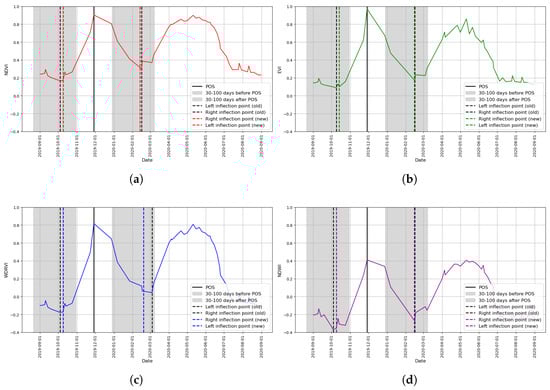
Figure 2.
Inflection point adjustment in time series derived from (a) NDVI, (b) EVI, (c) WDRVI, and (d) NDWI.
The first modification centered on accurately identifying the left and right inflection points surrounding the vegetative peak in the VITS. Agri-Phenopy’s original approach defined these inflection points as the minimum vegetation index values within a 30 to 100-day temporal window preceding and following the vegetative peak. Our observations, however, revealed that this method frequently generated imprecise inflection points. These inaccuracies were often attributable to the phenological behavior of cover crops or weeds, which obstructed the precise marking of the target crop’s emergence. Furthermore, the post-harvest VI plateau, a result of straw reflectance, often led to inflection points being identified long after the crop’s actual senescence due to reflectance by straw (Figure 2).
These limitations prompted us to employ a second modification, which we implemented by enhancing the algorithm’s ability to detect the inflection point. We did this by rounding up the identified minimum value within the 30 to 100-day window relative to the vegetative peak, i.e., 0.23146 and −0.13568 were rounded up to 0.24, and −0.13, respectively. The algorithm did this by searching for the data point whose value is closest to this rounded value within a defined tolerance of 0.01, starting from the temporal position of the vegetative peak. If such a value was found, its position in the time series was recorded as the inflection point. This refined procedure was used to determine both the left and right inflection points, with the objective of identifying the point that was temporally nearest to the vegetative peak. This refinement enhanced the accurate identification of inflection points that were relevant to the target crop’s phenological cycle (Figure 2). The third and last modification was performed by further adjusting Agri-Phenopy via the application of a double-logistic data smoothing function, after which the coefficient of determination () was used to evaluate the goodness of fit between the original and fitted curve (Figure 3).
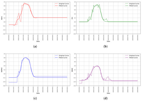
Figure 3.
Sample of vegetation index time series fitted with the (a) Savitz–Golay function (NDVI) (b) double-logistic function (EVI), (c), double-logistic function (WDRVI), and (d) double-logistic function (NDWI).
Approximately 10% of the plots exhibited poor fits due to the double-logistic function’s inability to find optimal parameters for the VITS. We addressed this limitation by applying the Savitzky–Golay filter [73] to curves with values that were below 0.8. This approach significantly reduced the percentage of poorly fitted curves from 10% to 0.2%. The window length, corresponding to the number of points used in the local polynomial fitting, was dynamically defined according to the available number of observations for each series, which was set at the highest odd value less than or equal to half the series length, with an upper limit of 51 points. A second-order polynomial was employed for the local regression, which helped by reducing noise reduction without losing the main characteristics and trends of the original signal. For example, in one sample, the double-logistic function adequately fitted the EVI (Figure 3b), WDRVI (Figure 3c), and NDWI (Figure 3d) time series, while the application of the Savitzky–Golay filter further improved the fit of the NDVI time series (Figure 3a).
2.6. Data Analysis
We adjusted the SOS dates detected by the algorithm to calibrate the sowing dates derived from VITS data by subtracting 10 days from each SOS date to account for the average time between sowing and emergence (i.e., sowing = SOS − 10 days) and by using the EOS dates as the harvest dates [74,75]. However, this period could be significantly longer, reaching up to 30 days for soybean sowing and for corn harvest. This was because, in general, these crops become detectable by satellites only after reaching their V3–V4 growth stages, a process whose timing was significantly affected by management and environmental variables such as weather conditions and soil type [76]. Therefore, we decided to explore intervals of −30 to 30 days for both SOS and EOS (Table 1).

Table 1.
Quantification of days applied for adjusting the dates of Start of Season and End of Season.
This choice was based on the analysis of the data distributions in relationship to the difference between the reference field data and the sowing date estimates derived from vegetation indices. We did this by selecting the day when the mean bias across all indices was closest to zero after detecting that, on average, more significant adjustments ranging from −15 days to −28 days were needed for SOS, while adjustments varying from −12 days to +16 days for EOS were reasoned to be necessary (Table 1).
For assessing the results, the Shapiro–Wilk (S-W) normality test [77], Mean Bias (MB), Standard Deviation of Bias (S.D. of Bias), Root Median Square Error (RMSE), Median Error (ME), and Spearman’s rank correlation coefficient [78] between the reference field data and the obtained estimates were used. Calculating the error using the median of the differences between predicted and reference data, instead of the mean, resulted in a measure that was more robust to outliers. This was because the median was less affected by extreme values than the mean. Additionally, the non-parametric Wilcoxon signed-rank test for paired samples [79] was applied to test for statistically significant differences between the RS-derived estimates and the field-observed data.
Finally, we observed that the results of the Wilcoxon test were significantly influenced by the adjustment day used to determine the SOS and EOS of the crop cycles. Given the possibility that different vegetation indices displayed distinct behaviors regarding the accuracy of phenological event detection, we applied the Wilcoxon test again to evaluate the use of individualized adjustments for each index, aiming to optimize the correspondence between phenological metrics derived from RS and the actual sowing and harvesting dates (Table 2).
Table 2.
Number of days adjusted for Start and End of Season for all vegetation indices combined and for each index individually.
It is important to note that, when available, farmers usually record sowing dates, but not the actual emergence dates of the crop. However, in many situations, reliable records of sowing dates are also lacking or incomplete. Moreover, RS algorithms typically detect the emergence dates, that is, the moment when green leaves become visible and can be distinguished by sensors. Because there is a variable delay between sowing and emergence, estimating sowing dates from RS data requires adjusting or translating the detected emergence dates to infer the actual sowing event. Therefore, algorithmically estimating sowing dates is an important challenge, especially when farmer records are missing, incomplete, or inconsistent. This gap was typically managed by assuming a fixed interval of days between sowing and plant emergence [74].
3. Results
Considering that we subtracted/added the same number of days to each metric, target crop, and study area, it is apparent that there was an unbiased comparison between vegetation indices (Table 1). We observed the lowest MB range for SOS in corn in PR, varying from −0.93 to 1.27. In contrast, corn in PR showed the greatest dispersion of MB values for EOS, ranging from −4.87 to 7.68. When considering the combined MB ranges for SOS and EOS, soybean in both PR and MT presented the smallest dispersion, with values ranging from −3.11 to 1.91 and from −2.32 to 2.76, respectively. These variations, although reflecting disparities among the indices used, do not show significant differences between them. MB measures the distance between predictions and reference data. Notably, for all study areas, NDVI exhibited the highest MB for sowing dates, while EVI showed the highest for harvest dates. (Table 3).
Table 3.
Summary of average errors in days of estimated phenology metrics by state and crop type.
The S. D. of Bias indicated average variations ranging from 9.72 to 14.51 days for SOS and from 10.76 to 26.76 days for EOS (Table 3). The S.D. of Bias measures the variability in the bias around the mean, with low values indicating that the differences between the predictions and the reference data are consistently close to the mean bias, indicating more reliable predictions. On the other hand, a high standard deviation indicates that the differences vary widely, suggesting lower reliability in the predictions. The results show that, for both SOS and EOS, none of the indices exhibited consistently low variability. However, it is worth noting that, for both SOS and EOS, the lowest S.D. of Bias values among the four indices evaluated were found in soybean areas in MT (Table 3).
Regarding EOS, it is worth noting that soybeans exhibited the lowest S.D. of Bias values, ranging from 10.76 to 13.18, while corn exhibited the highest S.D. of Bias values, ranging from 14.51 to 26.76. A similar pattern emerged during SOS, with soybean values ranging from 9.72 to 12.53 and those for corn ranging from 10.11 to 14.51. The only exception was for soybeans in PR, which exhibited an S.D. of bias of 12.53 days for the NDWI. Although the results demonstrate that, in general, the differences between the predictions and the reference data are consistently close to the mean bias, some uncertainties in the estimates can still be observed, especially when using the NDWI (Table 3).
This pattern was also observed for both RMSE and ME. For sowing, the RMSE and ME ranged from 5 to 6 days for soybeans, while values from 5 to 7 days were observed for corn. Once again, the exception was in PR using NDWI, which showed RMSE and ME values of 7 days for soybeans and 9 days for corn. For harvesting, RMSE and ME ranged from 6 to 7 days for soybeans and from 8 to 11 days for corn. The exceptions were soybeans in MT using EVI, which showed RMSE and ME values of 8 days, and corn in MT using EVI and NDWI, which showed RMSE and ME values of 14 and 15 days, respectively (Table 3).
The RMSE and ME for SOS ranged from 5 to 8 days across all vegetation indices (Table 3). For EOS, the RMSE and ME varied from 6 to 13 days for all indices. Due to the presence of outliers and the resulting potential for data bias, we chose to use the median RMSE and ME. Calculating the error using the median of the differences between the predicted and reference data, rather than the mean, provides a measure that is less affected by the external effects of outliers. This is because the median is less influenced by extreme values than the mean.
Following the S-W tests to assess the normality of data related to phenology metrics, both for the ground truth data on sowing and harvest and for the estimates using different vegetation indices (NDVI, EVI, WDRVI, NDWI), it was found that all samples led to the rejection of the null hypothesis of normality, using a significance level at .
This indicates that the data do not follow a normal distribution. Consequently, the Spearman correlation [78] was chosen for data analysis. Spearman’s rank correlation is a suitable non-parametric alternative, as it does not assume normal distributions and is effective for identifying monotonic relationships between the studied variables. It evaluates the strength and direction of these monotonic relationships between the variables, specifically between the estimates using vegetation indices and the ground truth data.
The Spearman correlation results indicate that all phenological metrics we extracted from the vegetation indices analyzed exhibit a strong and significant relationship with both sowing and harvesting dates (Figure 4, Figure 5, Figure 6 and Figure 7). Across all of the targeted study areas and for both crops, the vegetation indices consistently yielded moderate (0.50 to 0.75) to high (>0.75) Spearman correlation coefficients. These values not only reaffirm the validity of using vegetation indices such as NDVI, EVI, WDRVI, and NDWI for monitoring crop development but also highlight their value as practical tools for operational crop management. For soybeans in MT, the consistently high correlations for harvesting (0.82 to 0.83) indicate that these indices are highly effective in capturing the crop’s maturity, while the slightly lower but significant correlations for sowing (0.65 to 0.70) confirm their applicability in modeling the crop establishment and early growth stages (Figure 4).
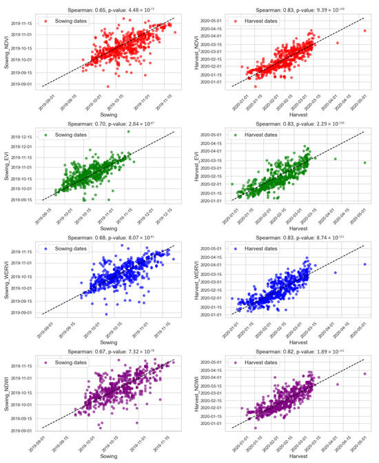
Figure 4.
Spearman correlation between observed field data and sowing/harvesting estimates for soybean in MT.
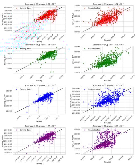
Figure 5.
Spearman correlation between observed field data and sowing/harvesting estimates for corn in MT.
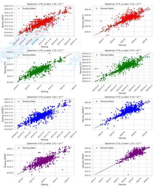
Figure 6.
Spearman correlation between observed field data and sowing/harvesting estimates for soybean in PR.
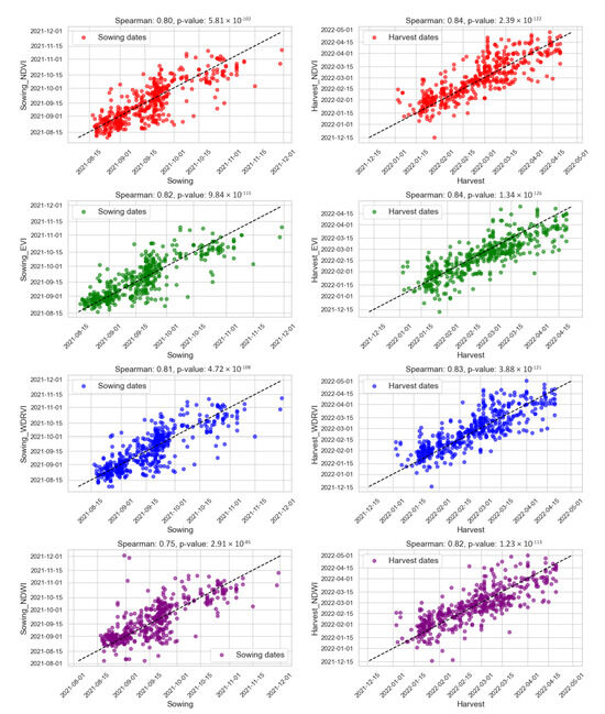
Figure 7.
Spearman correlation between observed field data and sowing/harvesting estimates for corn in PR.
For corn in MT, the Spearman correlation values ranged from 0.56 to 0.68 for both metrics, indicating moderate reliability for use in predictive models of sowing and harvest dates, though with some variability compared to other crop-area combinations. Correlations for sowing were marginally higher (0.65 to 0.68) compared to harvesting (0.56 to 0.61). Individual examination of the vegetation indices revealed that the NDVI presented a Spearman correlation of 0.66 for sowing and 0.61 for harvest, highlighting its consistent performance across both stages. The EVI showed similar reliability, with a coefficient of 0.65 for sowing and 0.61 for harvest, reinforcing its predictive potential. The WDRVI stood out with the highest correlation for sowing (0.68), though its harvest correlation was slightly lower (0.60). Lastly, the NDWI matched WDRVI for sowing (0.68), but produced the lowest correlation coefficient for harvest (0.56) among all indices (Figure 5).
For soybean in PR, the correlations remained consistently high for sowing (0.75 to 0.79) and harvest dates (0.72 to 0.75), highlighting that the vegetation indices robustly captured both phenological stages. The NDVI exhibited a correlation of 0.78 for sowing dates and 0.74 for harvest dates while the EVI produced the best results, with correlations of 0.79 for sowing and 0.75 for harvest. The WDRVI displayed a similar correlation to EVI for sowing (0.79), but a slight decrease was observed for harvest (0.72). The NDWI registered correlations of 0.75 for sowing and 0.72 for harvest. All indices exhibited consistent and stable performance for both sowing and harvesting, reinforcing their effectiveness across different crop stages (Figure 6).
Finally, for the first-season corn in PR, all the vegetation indices presented high Spearman correlations (>0.75). The correlations remained consistently high for harvesting (0.82 to 0.84), while high but slightly lower for sowing (0.75 to 0.82), with the marginal differences strongly suggesting that these indices also effectively captured both the sowing and harvesting.
The NDVI showed a correlation of 0.80 for sowing and a higher correlation of 0.84 for harvest. The EVI exhibited the highest values overall, with 0.82 for sowing and 0.84 for harvest, underscoring its superior performance throughout the crop cycle. The WDRVI also performed well, recording 0.81 for sowing and 0.83 for harvest. Lastly, the NDWI exhibited slightly lower values of 0.75 for sowing and 0.82 for harvest, which were, nevertheless, within acceptable limits. These results suggest that all of the indices we used were effective, with EVI and NDVI outperforming the others by accurately capturing both sowing and harvesting periods for corn in this region (Figure 7).
The results of the non-parametric Wilcoxon test revealed that the WDRVI, for the selected adjustment days, demonstrated the best performance, as it performed consistently in both study regions and for the crops (Figure 8). The Wilcoxon test statistics for the WDRVI, for both sowing and harvesting, showed higher values than the other indices, indicating that, in some cases, the differences observed between the predicted data and field data are not statistically significant. This suggests that the WDRVI, under the evaluated conditions, allows for more accurate estimates of phenological dates without introducing undesirable variations.
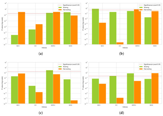
Figure 8.
Wilcoxon test p-values for sowing and harvesting with fixed start of season adjustment: (a) soybean in MT, (b) corn in MT, (c) soybean in PR, (d) corn in PR.
However, an important point to highlight is our observation that the adjustment of days between phenological metrics (SOS and EOS) and the actual sowing/harvesting dates directly influences the results of the Wilcoxon test. This finding motivated the evaluation of specific adjustments for each index, which led to a significant discovery: when the most appropriate adjustment was applied, the indices exhibited no statistically significant differences from the observed dates, as indicated by the results of the Wilcoxon test. Although we used a fixed adjustment for all indices (Table 1), varying only between states and crops, we tested adjustments for each index and arrived at the metrics previously shown in Table 2.
The analysis revealed that each state, crop, and vegetation index responds best to specific temporal adjustments. In the case of soybeans in MT, we initially applied a uniform correction of −18 days for the SOS and −12 days for the EOS for all four indices under consideration. Nonetheless, the ideal adjustments for SOS varied slightly among the indices: −18 days for NDVI, −20 days for EVI, −17 days for WDRVI, and −18 days for NDWI. Similarly, the optimal EOS corrections were determined as −12 days for NDVI, −9 days for EVI, −12 days for WDRVI, and −13 days for NDWI (Table 2).
For corn in MT, our general approach involved shifting SOS by −18 days and EOS by +9 days. However, a detailed assessment indicated that the best SOS adjustments were −18 days for NDVI, −19 days for both EVI and WDRVI, and −20 days for NDWI. Regarding EOS, the most suitable shifts were +5 days for NDVI, +18 days for EVI, +8 days for WDRVI, and +11 days for NDWI (Table 2).
We used an adjustment of −24 days for SOS and −7 days for EOS, considering soybeans in PR across all evaluated VITS. However, the best SOS adjustment was −23 days for NDVI, −26 days for EVI, −24 days for WDRVI, and −26 days for NDWI. In the case of EOS, the best adjustment was −6 days for NDVI, −5 days for EVI, −8 days for WDRVI, and −10 days for NDWI (Table 2).
For corn in PR, we used an adjustment of −28 days for SOS and −3 days for EOS, but the best SOS adjustment was −26 days for NDVI, −29 days for EVI, −28 days for WDRVI, and −26 days for NDWI. In the case of EOS, the best adjustment was 0 days for NDVI, 1 days for EVI, −1 days for WDRVI, and −3 days for NDWI (Table 2). These adjustments allowed all indices to exhibit high p-values, indicating that the observed differences were not statistically significant (Figure 9).
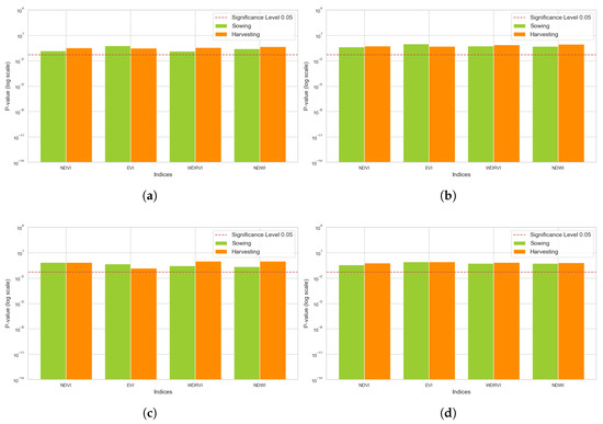
Figure 9.
Wilcoxon test p-values for sowing and harvesting with fixed start of season adjustment: (a) soybean in MT, (b) corn in MT, (c) soybean in PR, (d) corn in PR.
4. Discussion
Although inflection point–based empirical methods are common, a notable limitation is the occurrence of “false” inflection points, often caused by noise in the time series, especially from short-cycle cover crops sown before the target crop is planted. In addition, the use of fixed threshold values to determine dates does not always directly correspond to the actual physiological stages of the crop. For example, even though emergence is often considered to occur when a 10% increase in the VITS curve is observed, the actual emergence of many crops frequently takes place before any substantial change is detectable in the VITS. Studies have shown that, in the case of soybeans, for instance, the “visible” phenological detection in VITS typically corresponds to the V3–V4 stages, which mark the development of the third and fourth trifoliate leaves [76].
In light of these limitations, our methodology offers a substantial enhancement over traditional empirical methods. We chose a double-logistic function approach to model crop phenological development over the growing season, applying two logistic functions, one for the ascending and another for the descending phase of the VITS [44]. Crucially, the accuracy of our results is not simply the outcome of detecting left and right inflection points; instead, these inflection points served initially as delimiters, guiding and optimizing the fitting of the double-logistic function to the crop cycle. In addition, we implemented rigorous algorithmic modifications to refine inflection-point detection and, most importantly, employed an empirical calibration through a day adjustment step. This final adjustment is essential for translating remotely sensed dates of emergence and maturity into real-world agronomic events such as sowing and harvest. This calibration was key to overcoming the intrinsic variability between crop spectral response and the precise timing of agricultural operations, thereby demonstrating the robustness and practical applicability of our approach.
Building upon this methodological framework, VITS extracted from agricultural areas demonstrates behavioral variations throughout the entire crop cycle. Generally, vegetative development is represented by an ascending curve, while reproductive development is indicated by a descending curve. These contrarieties result in a characteristic behavior that enables the extraction of phenological metrics, which can be correlated with specific phenological stages. Based on this methodology, we evaluated whether the use of different vegetation indices improves the identification of sowing and harvesting dates. The sowing and harvesting dates were identified at the field scale through change detection in time series data from the HLS.
One of the major challenges in extracting phenological metrics from VITS in agricultural areas arises from the presence of multiple cropping cycles within the same agricultural year [80,81,82]. This becomes conspicuously evident when a target crop is cultivated in either the first or second cycle, depending on the producer’s decision.
In Brazil, common cropping sequences (e.g., soybean–corn or soybean–wheat in the South and Southeast; soybean–corn or soybean–cotton in the Central-West, North, and Northeast [48]) may compromise the performance of phenology-detection algorithms [83]. This problem was solved with our approach of defining a peak vegetative calendar for the target crop. If the peak was found within the defined interval, that cycle was identified as the target crop cycle. This enhanced performance in correctly defining the crop cycle.
The results indicate that, despite small variations in mean biases and RMSE, all indices have similar potential for applications in estimating sowing and harvesting dates, although each bears its own unique particularities regarding bias and precision. Overall, EVI presented the best results among the vegetation indices for phenology estimation, but biomass-rich areas did not result in performance gains for the estimation of sowing and harvesting dates.
It is interesting to note that the best performance when using EVI was also observed when various phenological metric extraction algorithms were tested [11]. Equally noteworthy is the fact that the metrics computed in our study were within reasonably acceptable limits. This finding is important because it highlights the need to develop phenological metric extraction algorithms that focus on agricultural areas [52]. Our methodology underscores the convenience and reliability of using RS data for timely assessment of crop phenological changes in the agricultural calendar, in lieu of costly, spatially restricted, and time-consuming in situ surveys.
Regarding RMSE and ME, all indices showed near-similar performance in the two regions and for both crops, with a marginal difference of ∼2 days between them. The exception was NDWI and EVI for corn harvest data in MT, which yielded results that were better than what the other indexes produced. These contrasting scenarios can be explained by the dynamics of the second-crop corn harvest in MT, which may have imparted the observed deviance of discrepant values.
A relevant aspect to consider is the relationship between the size of the fields and the number of pixels available for analysis in satellite images. Research has shown that constructing time series datasets for crops by selecting only the pixels that fall appropriately within the crop fields allows for the correct characterization of crop behavior, even in highly heterogeneous landscapes [84,85]. Smaller fields, such as those observed in PR (average of 33 ha), tend to contain a reduced number of pixels compared to the larger fields in MT (average of 227 ha). This difference has direct implications for the quality of the time series data used to estimate phenological events. Thus, the application of a border’s filter is strongly recommended in removing the mixed border pixels that diminish performance by compromising the consistent estimation of the phenology dates.
Understanding the limitations imposed by cloud cover is essential [86], especially because one of the main challenges in analyzing images of small crop fields is the interference caused by clouds. Since the approach used depends on HLS data, which already have a medium 30 m spatial resolution, cloud cover can further reduce the number of valid pixels available to compose the time series, as image masking is a crucial step in restricting the analysis to a subset of pixels in an area rather than using all pixels [87]. This effect tends to be more severe in smaller fields, where the removal of a reduced number of pixels due to cloud filtering can significantly compromise the continuity of the series, making it noisier and incapable of yielding reliable estimates.
The increased variability in the data linked with small crop fields directly impacts the accuracy of SOS and EOS estimates, increasing the uncertainty in calculations and effectuating higher RMSE and ME values for sowing, as observed in PR (6 to 8 days) compared to MT (5 to 6 days). In regions where the fields are larger, there is greater redundancy of information, allowing for more robust estimates and reducing the noise effects caused by gaps in the data. Thus, the difference in results between the states can largely be attributed to the difference in the analyzed field areas and the unavoidable unavailability of reliable data at appropriate temporal and spatial scales.
However, it should be noted that our results corroborate various approaches developed for the detection of phenological stages in corn and soybeans using VITS data. For example, methods that employed NDVI obtained from the HLS double-logistic function smoothed product achieved an RMSE of 8.2 days and ME of 6.1 days for soybeans, and an RMSE of 7.8 days and ME of 5.8 days for corn sowing dates [88]. A related approach, which used WDRVI derived from the MODIS sensor, reported an RMSE of 10.6 days for soybean sowing and 4.1 days for harvest, as well as an RMSE of 5.8 days for corn sowing and 11.0 days for harvest [39], while another study that used the EVI2 index on MODIS data produced an RMSE of 16 days for sowing and 17 days for harvest [11].
The use of HLS data in our study was crucial for obtaining robust results and reducing RMSE and ME, as some studies observed that estimates of phenological metrics can be affected by the temporal and spatial resolution of the sensor [11,89,90]. It was expected that altering the vegetation index used in the phenology estimates of crops using phenological metric extraction could have a greater impact than improving spatial and temporal resolution, with this expectation being premised on observations by [11]. This is likely related to the different purposes for which each vegetation index is computed. While the WDRVI was developed as an alternative to overcome NDVI saturation issues [34], the EVI was designed to address not only saturation but also to minimize atmospheric contamination and to reduce the exposed soil signal present in the NDVI [58]. The NDWI was proposed for the measurement and monitoring of liquid water content in vegetation [35]. However, our findings reinforce that the use of different indices does not have a significant impact on the results, as long as the day adjustment is appropriate for each index.
Regarding day adjustment, an important point in using phenological metrics for estimating phenological stages is the fact that SOS is related to the emergence date and not the sowing date. Since, in general, producers have records of the sowing date and not the emergence date, it is necessary to consider this difference. Although the literature suggests using 10 days [74,75], our study demonstrated that a 10-day fixed periodization would lead to lower accuracy and higher errors.
However, the SOS date can vary according to the sowing depth, seed vigor, amount of straw covering the soil, weather/climatic conditions like temperature, soil moisture, and even its texture (i.e., clay percentage), in addition to the presence/absence of compaction [91,92,93]. These are physical and physiological impediments that can influence the interval between sowing and crop emergence. Soils with a high clay content e.g., tend to delay the emergence date of crops by acting as a physical barrier, [94] while an excess of crop residue also has a negative correlation with the number of days between planting and seed emergence [91].
Another factor is the depth of sowing, which can affect the average time of emergence for both soybeans [91] and corn [91,92]. Furthermore, climatic conditions such as low soil moisture and/or low temperatures can reduce the physiological activity of the seed and delay emergence [93]. We tested different intervals (−30 to 30 days) from the actual sowing date and the SOS. The discrepancies observed between the estimates can be attributed to errors between the RS data and field measurements. In our study, the best day intervals for deriving the sowing date from SOS varied depending on the targeted area and crop, ranging from 17 to 29 days.
In general, most studies estimating harvest report that the EOS date has a high correlation with the crop’s harvest date. In our analyses, we considered EOS as the harvest date for the target crop, but we conducted some tests with a few days of adjustment and found that adjusting the EOS date (ranging from 0 to 18 days) can considerably improve the results.
In determining the sowing date for soybeans and corn in MT, the best results were obtained by reducing the SOS date by 18 days. That may indicate a period variation of ±18 days from the sowing date to the detected emergency through the SOS. However, for the harvest, the best results were achieved by reducing the EOS date for soybeans by 12 days, while for corn it was necessary to add an average of 9 days to the EOS date.
A particular aspect of the second-crop corn cultivation in MT is that the state has a deficit in grain storage, forcing producers to move their production right after harvesting [95]. The soybeans grown in the state are quickly harvested (January–March), dried, and transported to the ports [96]. This process ensures that storage capacity is available for the second-crop corn, which is subsequently harvested between May and July. However, a delay in soybean sowing, difficulty in commercialization, and logistical constraints can delay the flow of soybeans, directly impacting the available static storage capacity [97].
In this context, producers may choose to keep the corn ready for harvest (R6) still in the field. Although this can lead to moisture (and weight) loss, it is a viable coping strategy when there is no place for storage. That said, the extraction of EOS is related to the moment when the target crop is ready for harvest (R6) and not exclusively to the moment it was harvested. Thus, the harvest date is, on average, a few days ahead of the EOS date. For this reason, it was necessary to add 11 days for corn, while for soybeans, it was necessary to reduce EOS by 12 days.
In addition to the need to plant second-crop corn immediately after the soybean harvest, it is important to note that this period is marked by frequent rainfall in the state, which makes a quick soybean harvest necessary both to optimize the agricultural calendar and to prevent grain quality losses due to excessive moisture. This is different from the second-crop corn, which reaches full maturity during the dry rain-free winter period, which allows delayed harvesting.
In estimating sowing and harvest dates in PR, the best results were obtained by reducing the SOS date by 24 days for soybeans and 28 days for corn. However, for the harvest, it was necessary to reduce the EOS date by 7 days for soybeans and 3 days for corn. An important point here is that, in PR, using samples of first-crop corn, sowing and harvest occur in the same calendar period/months as soybeans. In MT, we used samples of second-crop corn, which is sown after the soybean harvest. This temporal coincidence explains the similar values observed for soybeans (24 days for SOS and 7 days for EOS) and corn (28 days for SOS and 3 days for EOS). Furthermore, since it is sown as the first crop, corn needs to be harvested quickly to make way for winter crops. For this reason, it was necessary to reduce (and not increase) the EOS adjustment in days in PR.
Essentially, detecting the sowing date for soybeans is generally more difficult to predict than the harvest date. In addition to the factors mentioned that can interfere with the sowing and emergence dates, the development of soybean crops, for example, usually only becomes detectable in VITS around the V3 stage (third node) [76]. The V3 stage typically occurs 12 to 25 days after emergence [98]. For corn, detection occurs around the same V3 stage (third leaf) [37] and usually occurs ∼7 days after emergence [99].
After emergence, the phenological behavior of crops is influenced by the seasonal effects of precipitation, temperature, and photoperiod [100]. In some cases, even management practices can alter phenology, such as the application of fungicides, which can promote greater accumulation of dry matter and leaf area, or a longer period of maintaining the photosynthetically active area, which can alter phenology by modifying and lengthening the phenological cycle [101]. This can result in later-than-expected harvests, but since the VITS behavior is also expected to decline marginally, correctly identifying EOS becomes less problematic.
A common practice in soybean fields is desiccation. This technique aims to minimize the negative influence of biotic and abiotic factors on seed physiological quality at the end of the plant cycle [102]. This management intervention involves the application of desiccant herbicides near the end of the crop cycle to accelerate senescence and the drying of the plants. If the practice is applied to the entire field rather than just the borders, it leads to an earlier harvest [103], which can introduce errors in EOS estimates. However, much like the application of fungicides, the behavior of VITS is also expected to change (more pronounced decline), and it should not significantly affect EOS identification.
These results highlight the importance of regional and crop-specific calibration of RS-based methods, aiming to increase accuracy in the monitoring of crop phenology and to minimize discrepancies that can arise from the use of generalized algorithms. All the factors described in the preceding paragraphs, and many others that are beyond the scope of this investigation, provide a plausible explanation of why the adjustment days were smaller for EOS (0 to 18 days) and larger for SOS (17 to 29 days). Additionally, it is worth noting that the results of the Spearman correlations were higher for EOS (0.72 to 0.85) and lower for SOS (0.53 to 0.79), as reported in another study where the Spearman correlation was 0.76 for soybean harvest, while it was 0.71 for sowing using the EVI2 index in MODIS data [11].
This occurs because, after reaching its vegetative peak, the plant enters a senescence stage but continues developing until harvest with few significant changes. Although climatic and management conditions can influence the harvest date to some extent, it generally tends to remain stable, which explains the higher correlation values observed for the harvest.
Additionally, for sowing using NDVI, the Spearman correlation was lower for soybeans (0.72) than for corn (0.73). These results are consistent with what other researchers observed in a study in which they derived field-level planting dates for corn and soybean in the US Midwest by using NDVI derived from the HLS double-logistic function smoothed product, with their results showing a Spearman correlation of 0.69 for corn and 0.62 for soybeans [88].
Still, regarding the best day adjustment for SOS, NDVI is more sensitive for detecting green vegetation, even in areas with low vegetation cover, quickly detecting the reflectance of the vegetation cover [32]. This is due to its sensitivity to changes in the red and near-infrared reflectance, which increase significantly when plants begin to germinate and develop leaves. This may explain why on average, NDVI required the smallest adjustment for SOS (−21 days, on average). By using the same bands, WDRVI allowed for an adjustment close to NDVI (−22 days, on average). However, it still required slightly more time due to its dependence on spectral reflectance from areas with high biomass [34].
NDWI and EVI were the indices that required the greatest adjustment of days (−23 and −24 days) for SOS, respectively. Since NDWI responds well to the water content in plants [35], the spectral response can be limited at stages of low biomass. At the beginning of the cycle, the crops are still emerging and may not have enough biomass to induce a significant variation in NDWI.
Regarding the EVI, what is worth noting is that it may have required larger SOS adjustments due to its architectural dependence on atmospheric and soil correction, lower sensitivity to low biomass, greater sensitivity to canopy closure [33], or a combination of these factors. EVI is designed to minimize soil and atmospheric effects, which makes it less sensitive in areas with low vegetation, which is common at the beginning of the crop cycle. Since EVI uses the blue band to correct atmospheric and soil influence, it tends to saturate less than NDVI [104] but tends to be less responsive in early stages when biomass is low. Stated differently, although EVI responds better to active vegetation growth compared to NDVI, for example, its performance in the identification of crop emergence is dependent on biomass accumulation. This dependence might have delayed early detection of SOS.
EVI showed the smallest day adjustment for EOS (1 day), probably because EVI is sensitive to changes in canopy structure and leaf conditions, making it useful for detecting early maturation. NDVI and WDRVI are less effective at the end of the season when senescence begins, as the near-infrared reflectance decreases slowly. This explains why larger adjustments were necessary (3 and −3 days for NDVI e WDRVI, respectively) to capture EOS. At the end of the cycle, even after reaching full maturity, there is still water in the plant and grain structure, justifying a larger EOS adjustment for NDWI (−4 days), hence its detection of season’s end later than the other indices.
As expected, on average, SOS required more adjustment than EOS, which is why some studies in the literature recommend a −10 day adjustment for SOS and 0 days for EOS. However, our results showed that various factors can influence the number of days between sowing and emergence, which directly affects the number of days needed for adjustment. Additionally, there are cases in which harvest occurs later when storage facilities are not available, such as for second-crop corn in MT. Conversely, there are cases where harvest occurs earlier, as when the corn is intended for silage, such as first-crop corn in PR.
5. Conclusions
Extreme weather events, intensified by climate change, represent a significant threat to global food security. Consequently, accurately estimating the phenological stages of crops has become an urgent necessity for decision-making throughout the entire production chain. The information obtained from these estimates is essential for the efficient management of food production, allowing for more resilient and adaptive planning in the face of climate challenges. This is because reliable and timely provisioning of information on sowing and harvest dates enables farmers to minimize the risks of climate change-driven crop failures.
Accomplishing this is not only necessary but indispensable in a world where secure access to adequate food supplies is steadily diminishing, mostly due to adverse effects of unpredictable external factors such as increased frequency of rainfall failures and heat waves. Mitigating these threats in the context of reliable and sustainable access to adequate food supplies requires the aforementioned information on sowing and harvest dates.
These observations argue for the need to explore innovative techniques that can be used to support agriculture by providing some of the critical information that is required in this sector. We attempted to do this by providing an improvised methodology that is potentially capable of enhancing our capacities to cope with the adverse effects of climate change by supporting the timely provisioning of usable information on crop sowing and harvest dates. We did this by tapping on purposefully selected indices that include NDVI, EVI, WDRVI, and NDWI, as illustratively described in this paper. The following highlights provide a snapshot overview of the major insights from our pilot initiative.
Although differences were observed among the tested vegetation indices, all showed quite robust results. Depending on the information needed, any of these indices can be used without significant drawbacks for subsequent analyses. However, we emphasize the importance of making specific adjustments to optimize analytical performance, ensuring even more precise and reliable results.
Despite the similarity among the indices, NDVI demonstrated the best overall performance across all analyses. Based on our results, its advantages include requiring smaller day adjustments on average, achieving the highest Spearman correlations, showing the lowest S.D. of bias, RMSE, and ME, and producing the fewest outliers. Additionally, because it uses only the NIR and red bands, which are common across most sensors, NDVI is the most recommended index for crop-phenology studies.
We were able to demonstrate that adjusting the days applied to SOS and EOS to estimate sowing and harvest dates, respectively, can be crucial in improving forecasts and the results of different processing procedures. Future studies can further explore this field, offering new perspectives and improvements.
These adjustments not only increase the accuracy of phenological estimates but also ensure that forecasts are consistent across different regions and crops. This level of detail is particularly important in agricultural contexts, where information accuracy can significantly impact yield estimation and decision-making. Furthermore, recognizing that customized adjustments by index are beneficial suggests that future research could explore automating these processes, leveraging machine learning technologies to further optimize phenological forecasts.
Additional studies that use different vegetation indices and data sources can significantly contribute to improving the accuracy of phenological estimates. There is still room for improvements, such as the application of smoothing techniques, like wavelets, which can help reduce outliers often associated with VITS adjustment. Despite the limitations, this study represents a significant advance in the use of phenological metrics to estimate the phenological stages of crops.
Our take-home message is that, although challenges undermining the unrestricted provision of vital information on agriculture persist, they can still be confronted and addressed. This can be achieved by embracing collective efforts to explore and implement innovative techniques that bridge the information gaps that undermine our ability to cope with and adapt to the adverse effects of wide-ranging stressors. We conclude by highlighting the need for ongoing collaboration among researchers and stakeholders to place this challenge at the forefront, ensuring that innovative solutions continue to be developed for the benefit of agricultural resilience.
Supplementary Materials
The following supporting information can be downloaded at https://www.mdpi.com/article/10.3390/rs17172927/s1. Figure S1: A roadmap of the stages of crop phenology derived from HLS time series.
Author Contributions
Conceptualization, C.T.C.d.S., M.A. and M.M.C.; methodology, C.T.C.d.S., M.A. and V.H.R.P.; software, C.T.C.d.S., M.A. and V.H.R.P.; validation, C.T.C.d.S. and M.A.; formal analysis, C.T.C.d.S., M.A. and V.H.R.P.; investigation, C.T.C.d.S. and A.D.B.G.; resources, C.T.C.d.S. and A.D.B.G.; data curation, C.T.C.d.S.; writing—original draft preparation, C.T.C.d.S. and M.A.; writing—review and editing, C.T.C.d.S., M.A., M.M.C., V.H.R.P. and A.D.B.G.; visualization, C.T.C.d.S.; supervision, M.A., M.M.C. and V.H.R.P.; project administration, C.T.C.d.S. and M.A.; funding acquisition, C.T.C.d.S. and M.A. All authors have read and agreed to the published version of the manuscript.
Funding
This research was funded in part by the Brazilian Federal Agency for Support and Evaluation of Graduate Education (CAPES), Brazil; Finance Code 001. The authors are grateful to the Brazilian National Council of Scientific and Technological Development (CNPq) for the Research Productivity Fellowship of Adami, M. [PQ 309045/2023-1].
Institutional Review Board Statement
Not applicable.
Informed Consent Statement
Not applicable.
Data Availability Statement
Restrictions apply to the availability of the dataset used for analysis. The data were obtained from SLC Agricola S.A. and ABC Foundation and are not available.
Acknowledgments
Special thanks to SLC Agricola S.A. and ABC Foundation for providing a comprehensive database containing crop field geometries and precise information on sowing and harvest dates.
Conflicts of Interest
Author Cleverton Tiago Carneiro de Santana was employed by the National Food Supply Company (CONAB), SGAS I Setor de Grandes Áreas Sul 901 s/n, Asa Sul, Brasília 70390-010, DF, Brazil. The remaining authors declare that the research was conducted in the absence of any commercial or financial relationships that could be construed as a potential conflict of interest.
Abbreviations
The following abbreviations are used in this manuscript:
| BRDF | Bidirectional Reflectance Distribution Function |
| EVI | Enhanced Vegetation Index |
| HLS | Harmonized Landsat Sentinel-2 |
| MB | Mean Bias |
| ME | Median Error |
| MT | Mato Grosso |
| MODIS | Moderate Resolution Imaging Spectroradiometer |
| MSI | MultiSpectral Instrument |
| NDVI | Normalized Difference Vegetation Index |
| NDWI | Normalized Difference Water Index |
| OLI | Operational Land Imager |
| PR | Paraná |
| RMSE | Root Median Square Error |
| RS | Remote Sensing |
| S.D. of Bias | Standard Deviation of Bias |
| S-W | Shapiro–Wilk |
| VITS | Vegetation Index Time Series |
| WDRVI | Wide Dynamic Range Vegetation Index |
| ZARC | Agricultural Climate Risk Zoning |
References
- Burli, P.H.; Nguyen, R.T.; Hartley, D.S.; Griffel, L.M.; Vazhnik, V.; Lin, Y. Farmer characteristics and decision-making: A model for bioenergy crop adoption. Energy. 2021, 234, 121235. [Google Scholar] [CrossRef]
- Hyles, J.; Bloomfield, M.T.; Hunt, J.R.; Trethowan, R.M.; Trevaskis, B. Phenology and related traits for wheat adaptation. Heredity. 2020, 125, 417–430. [Google Scholar] [CrossRef]
- He, L.; Jin, N.; Yu, Q. Impacts of climate change and crop management practices on soybean phenology changes in China. Sci. Total Environ. 2020, 707, 135638. [Google Scholar] [CrossRef] [PubMed]
- Anand, S.; Barua, M.K. Modeling the key factors leading to post-harvest loss and waste of fruits and vegetables in the agri-fresh produce supply chain. Comput. Electron. Agric. 2022, 198, 106936. [Google Scholar] [CrossRef]
- Flohr, B.M.; Hunt, J.R.; Kirkegaard, J.A.; Evans, J.R. Water and temperature stress define the optimal flowering period for wheat in south-eastern Australia. Field Crops Res. 2017, 209, 108–119. [Google Scholar] [CrossRef]
- Guo, Z. Mapping the planting dates: An effort to retrive crop phenology information from MODIS NDVI time series in Africa. In Proceedings of the International Geoscience and Remote Sensing Symposium, Melbourne, VIC, Australia, 21–26 July 2013; pp. 3281–3284. [Google Scholar]
- Duchemin, B.; Fieuzal, R.; Rivera, M.A.; Ezzahar, J.; Jarlan, L.; Rodriguez, J.C.; Hagolle, O.; Watts, C. Impact of sowing date on yield and water use efficiency of wheat analyzed through spatial modeling and FORMOSAT-2 images. Remote Sens. 2015, 7, 5951–5979. [Google Scholar] [CrossRef]
- Urban, D.; Guan, K.; Jain, M. Estimating sowing dates from satellite data over the US midwest: A comparison of multiple sensors and metrics. Remote Sens. Environ. 2018, 211, 400–412. [Google Scholar] [CrossRef]
- Santana, C.T.C.; Sanches, I.D.A.; Caldas, M.M.; Adami, M. A method for estimating soybean sowing, beginning seed, and harvesting dates in Brazil using NDVI-MODIS data. Remote Sens. 2024, 16, 2520. [Google Scholar] [CrossRef]
- Sacks, W.J.; Deryng, D.; Foley, J.A.; Ramankutty, N. Crop planting dates: An analysis of global patterns. Glob. Ecol. Biogeogr. 2010, 19, 607–620. [Google Scholar] [CrossRef]
- Rodigheri, G.; Sanches, I.D.A.; Richetti, J.; Tsukahara, R.Y.; Lawes, R.; Bendini, H.D.N.; Adami, M. Estimating crop sowing and harvesting dates using satellite vegetation index: A comparative analysis. Remote Sens. 2023, 15, 5366. [Google Scholar] [CrossRef]
- Hochman, Z.; Gobbett, D.; Holzworth, D.; McClelland, T.; Rees, H.V.; Marinoni, O.; Garcia, J.N.; Horan, H. Quantifying yield gaps in rainfed cropping systems: A case study of wheat in Australia. Field Crops Res. 2012, 136, 85–96. [Google Scholar] [CrossRef]
- Jain, M.; Srivastava, A.K.; Joon, R.K.; McDonald, A.; Royal, K.; Lisaius, M.C.; Lobell, D.B. Mapping smallholder wheat yields and sowing dates using microsatellite data. Remote Sens. 2016, 8, 860. [Google Scholar] [CrossRef]
- Brazil. Decree No. 9841, of 18 June 2019: Provides for the National Program for Agricultural Zoning of Climate Risk (ZARC). Available online: https://www.planalto.gov.br/ccivil_03/_ato2019-2022/2019/decreto/d9841.htm (accessed on 30 June 2024).
- Manfron, G.; Delmotte, S.; Busetto, L.; Hossard, L.; Ranghetti, L.; Brivio, P.A.; Boschetti, M. Estimating inter-annual variability in winter wheat sowing dates from satellite time series in Camargue, France. Int. J. Appl. Earth Obs. Geoinf. 2017, 57, 190–201. [Google Scholar]
- Marinho, E.; Vancutsem, C.; Fasbender, D.; Kayitakire, F.; Pini, G.; Pekel, J.F. From remotely sensed vegetation onset to sowing dates: Aggregating pixel-level detections into village-level sowing probabilities. Remote Sens. 2014, 6, 10947–10965. [Google Scholar] [CrossRef]
- Lobell, D.B.; Ortiz-Monasterio, J.I.; Sibley, A.M.; Sohu, V.S. Satellite detection of earlier wheat sowing in India and implications for yield trends. Remote Sens. 2013, 115, 137–143. [Google Scholar] [CrossRef]
- Sakamoto, T.; Yokozawa, M.; Toritani, H.; Shibayama, M.; Ishitsuka, N.; Ohno, H. A crop phenology detection method using time-series MODIS data. Remote Sens. Environ. 2005, 96, 366–374. [Google Scholar] [CrossRef]
- Silva, A.A.; Silva, F.C.D.S.; Guimarães, C.M.; Saleh, I.A.; Crus Neto, J.F.; El-Tayeb, M.A.; Abdel-Maksoud, M.A.; Aguilera, J.G.; Abdelgawad, H.; Zuffo, A.M. Spectral indices with different spatial resolutions in recognizing soybean phenology. PLoS ONE 2024, 19, 1–21. [Google Scholar] [CrossRef]
- Gao, F.; Zhang, X. Mapping crop phenology in near real-time using satellite remote sensing: Challenges and opportunities. J. Remote Sens. 2021, 2021, 1–14. [Google Scholar] [CrossRef]
- Gao, F.; Anderson, M.; Daughtry, C.; Karnieli, A.; Hively, D.; Kustas, W. A within-season approach for detecting early growth stages in corn and soybean using high temporal and spatial resolution imagery. Remote Sens. Environ. 2020, 242, 111752. [Google Scholar] [CrossRef]
- Li, J.; Roy, D.P. A global analysis of Sentinel-2A, Sentinel-2B and Landsat-8 data revisit intervals and implications for terrestrial monitoring. Remote Sens. 2017, 9, 902. [Google Scholar] [CrossRef]
- Lulla, K.; Nellis, M.D.; Rundquist, B. The Landsat 8 is ready for geospatial science and technology researchers and practitioners. Geocarto Int. 2013, 28, 191. [Google Scholar] [CrossRef]
- Lulla, K.; Nellis, M.D.; Rundquist, B.; Srivastava, P.K.; Szabo, S. Mission to earth: Landsat 9 will continue to view the world. Geocarto Int. 2021, 36, 2261–2263. [Google Scholar] [CrossRef]
- Roy, D.P.; Wulder, M.A.; Loveland, T.R.; Woodcock, C.E.; Allen, R.; Anderson, M.; Helder, D.; Irons, J.R.; Johnson, D.M.; Kennedy, R.; et al. Landsat-8: Science and product vision for terrestrial global change research. Remote Sens. Environ. 2014, 145, 154–172. [Google Scholar] [CrossRef]
- Whitcraft, A.K.; Becker-Reshef, I.; Killough, B.D.; Justice, C.O. Meeting earth observation requirements for global agricultural monitoring: An evaluation of the revisit capabilities of current and planned moderate resolution optical earth observing missions. Remote Sens. 2015, 7, 1482–1503. [Google Scholar] [CrossRef]
- Claverie, M.; Ju, J.; Masek, J.G.; Dungan, J.L.; Vermote, E.F.; Roger, J.C.; Skakun, S.V.; Justice, C. The Harmonized Landsat and Sentinel-2 surface reflectance data set. Remote Sens. Environ. 2018, 219, 145–161. [Google Scholar] [CrossRef]
- Zhou, Q.; Rover, J.; Brown, J.; Worstell, B.; Howard, D.; Wu, Z.; Gallant, A.L.; Rundquist, B.; Burke, M. Monitoring landscape dynamics in central U.S. grasslands with Harmonized Landsat-8 and Sentinel-2 time series data. Remote Sens. 2019, 11, 328. [Google Scholar] [CrossRef]
- Jönsson, P.; Cai, Z.; Melaas, E.; Friedl, M.A.; Eklundh, L. A method for robust estimation of vegetation seasonality from Landsat and Sentinel-2 time series data. Remote Sens. 2018, 10, 635. [Google Scholar] [CrossRef]
- Vrieling, A.; Meroni, M.; Darvishzadeh, R.; Skidmore, A.K.; Wang, T.; Zurita-Milla, R.; Oosterbeek, K.; O’Connor, B.; Paganini, M. Vegetation phenology from Sentinel-2 and field cameras for a Dutch barrier island. Remote Sens. Environ. 2018, 215, 517–529. [Google Scholar] [CrossRef]
- Zeng, L.; Wardlow, B.D.; Xiang, D.; Hu, S.; Li, D. A review of vegetation phenological metrics extraction using time-series, multispectral satellite data. Remote Sens. Environ. 2020, 237, 111511. [Google Scholar] [CrossRef]
- Rouse, J.W.; Hass, R.H.; Schell, J.A.; Deering, D.W. Monitoring vegetation systems in the great plains with ERTS. In Proceedings of the Earth Resources Technology Satellite-1 Symposium, Washington, DC, USA, 10–14 December 1973; ERTS. pp. 309–317. [Google Scholar]
- Liu, H.Q.; Huete, A. A feedback based modification of the NDVI to minimize canopy background and atmospheric noise. IEEE Trans. Geosci. Remote Sens. 1995, 33, 457–465. [Google Scholar] [CrossRef]
- Gitelson, A.A. Wide dynamic range vegetation index for remote quantification of biophysical characteristics of vegetation. Agric. For. Meteorol. 2004, 161, 165–173. [Google Scholar] [CrossRef]
- Gao, B.C. NDWI—A normalized difference water index for remote sensing of vegetation liquid water from space. Remote Sens. Environ. 1996, 58, 257–266. [Google Scholar] [CrossRef]
- Diao, C.; Yang, Z.; Gao, F.; Zhang, X.; Yang, Z. Hybrid phenology matching model for robust crop phenological retrieval. ISPRS J. Photogramm. Remote Sens. 2021, 181, 308–326. [Google Scholar] [CrossRef]
- Sakamoto, T.; Wardlow, B.D.; Gitelson, A.A.; Verma, S.B.; Suyker, A.E.; Arkebauer, T.J. A two-step filtering approach for detecting maize and soybean phenology with time-series MODIS data. Remote Sens. Environ. 2010, 114, 2146–2159. [Google Scholar] [CrossRef]
- Liu, L.; Cao, R.; Chen, J.; Shen, M.; Wang, S.; Zhou, J.; He, B. Detecting crop phenology from vegetation index time-series data by improved shape model fitting in each phenological stage. Remote Sens. Environ. 2022, 277, 113060. [Google Scholar] [CrossRef]
- Sakamoto, T. Refined shape model fitting methods for detecting various types of phenological information on major U.S. crops. ISPRS J. Photogramm. Remote Sens. 2018, 138, 176–192. [Google Scholar] [CrossRef]
- Cao, R.; Li, L.; Liu, L.; Liang, H.; Zhu, X.; Shen, M.; Zhou, J.; Li, Y.; Chen, J. A spatiotemporal shape model fitting method for within-season crop phenology detection. ISPRS J. Photogramm. Remote Sens. 2024, 217, 179–198. [Google Scholar] [CrossRef]
- Cao, R.; Chen, J.; Shen, M.; Tang, Y. An improved logistic method for detecting spring vegetation phenology in grasslands from MODIS EVI time-series data. Agric. For. Meteorol. 2015, 200, 9–20. [Google Scholar] [CrossRef]
- Bolton, D.K.; Friedl, M.A. Forecasting crop yield using remotely sensed vegetation indices and crop phenology metrics. Agric. For. Meteorol. 2013, 173, 74–84. [Google Scholar] [CrossRef]
- Boschetti, M.; Stroppiana, D.; Brivio, P.A.; Bocchi, S. Multi-year monitoring of rice crop phenology through time series analysis of MODIS images. Int. J. Remote Sens. 2009, 30, 4643–4662. [Google Scholar] [CrossRef]
- Zhang, X.; Friedl, M.A.; Schaaf, C.B.; Strahler, A.H.; Hodges, J.C.; Gao, F.; Reed, B.C.; Huete, A. Monitoring vegetation phenology using MODIS. Remote Sens. Environ. 2003, 84, 471–475. [Google Scholar] [CrossRef]
- Diao, C. Remote sensing phenological monitoring framework to characterize corn and soybean physiological growing stages. Remote Sens. Environ. 2020, 248, 111960. [Google Scholar] [CrossRef]
- IBGE-Instituto Brasileiro de Geografia e Estatística. 2019 Biomes and Coastal-Marine System of Brazil. Available online: https://www.ibge.gov.br/geociencias/informacoes-ambientais/vegetacao/15842-biomas.html (accessed on 18 July 2023).
- Abrahão, G.M.; Costa, M.H. Evolution of rain and photoperiod limitations on the soybean growing season in Brazil: The rise (and possible fall) of double-cropping systems. Agric. For. Meteorol. 2018, 256, 32–45. [Google Scholar] [CrossRef]
- CONAB-Companhia Nacional de Abastecimento. 2022 Grain Sowing and Harvest Calendar in Brazil. Available online: https://www.gov.br/conab/pt-br/acesso-a-informacao/institucional/publicacoes/arquivos-de-paginas/calendariozplantiozezcolheitazjunz2022.pdf (accessed on 26 October 2023).
- Juliatti, F.C.; Zambolim, L. Etiology, epidemiology and management of Asian Soybean Rust (ASR) in Brazil and vulnerability of chemical control of specific without multisite fungicides. In Cereal Grains; Goyal, A.K., Ed.; RAYN Cultivation: Hershey, PA, USA, 2021; pp. 41–60. [Google Scholar]
- NASA-National Aeronautics and Space Administration. NASA’s Earthdata Search. Available online: https://search.earthdata.nasa.gov/ (accessed on 21 February 2024).
- Beck, P.S.; Atzberger, C.; Høgda, K.A.; Johansen, B.; Skidmore, A.K. Improved monitoring of vegetation dynamics at very high latitudes: A new method using MODIS NDVI. Remote Sens. Environ. 2006, 100, 321–334. [Google Scholar] [CrossRef]
- Santana, C.T.C.; Sanches, I.D.; Adami, M.A.; Caldas, M.M.; Oldoni, L.V. Agri-phenopy: An algorithm for extracting agricultural crops phenology metrics from vegetation index time series. In Proceedings of the Anais of the XXI Brazilian Remote Sensing Symposium, Salvador, BA, Brazil, 13–16 April 2025; Available online: https://proceedings.science/sbsr-2025/papers/agri-phenopy-an-algorithm-for-extracting-agricultural-crops-phenology-metrics-fr?lang=en (accessed on 16 May 2024).
- Franch, B.; Vermote, E.; Skakun, S.; Roger, J.C.; Masek, J.; Ju, J.; Villaescusa-Nadal, J.L.; Santamaria-Artigas, A. A method for Landsat and Sentinel 2 (HLS) BRDF normalization. Remote Sens. 2019, 11, 632. [Google Scholar] [CrossRef]
- Masek, J.G.; Ju, J.; Skakun, S.V.; Roger, J.C.; Vermote, E.F.; Claverie, M.; Dungan, J.L.; Yin, Z.; Freitag, B.; Justice, C.O. HLS Sentinel-2 MSI Surface Reflectance Daily Global 30m v2.0. NASA EOSDIS Land Processes DAAC 2021, 2. Available online: https://www.earthdata.nasa.gov/data/catalog/lpcloud-hlss30-1.5 (accessed on 17 August 2025).
- Masek, J.G.; Ju, J.; Skakun, S.V.; Roger, J.C.; Vermote, E.F.; Claverie, M.; Dungan, J.L.; Yin, Z.; Freitag, B.; Justice, C.O. HLS Operational Land Imager Surface Reflectance and TOA Brightness Daily Global 30 m v2.0. NASA EOSDIS Land Processes DAAC 2021, 2. Available online: https://cmr.earthdata.nasa.gov/search/concepts/C2021957657-LPCLOUD.html (accessed on 17 August 2025).
- Zhu, Z.; Wang, S.; Woodcock, C.E. Improvement and expansion of the fmask algorithm: Cloud, cloud shadow, and snow detection for Landsats 4–7, 8, and Sentinel-2 images. Remote Sens. Environ. 2015, 159, 269–277. [Google Scholar] [CrossRef]
- Qiu, S.; Zhu, Z.; He, B. Fmask 4.0: Improved cloud and cloud shadow detection in Landsats 4–8 and Sentinel-2 imagery. Remote Sens. Environ. 2019, 231, 111205. [Google Scholar] [CrossRef]
- Huete, A.; Didan, K.; Miura, T.; Rodriguez, E.P.; Gao, X.; Ferreira, L.G. Overview of the radiometric and biophysical performance of the MODIS vegetation indices. Remote Sens. Environ. 2002, 83, 195–213. [Google Scholar] [CrossRef]
- Seo, B.; Lee, J.; Lee, K.D.; Hong, S.; Kang, S. Improving remotely-sensed crop monitoring by NDVI-based crop phenology estimators for corn and soybeans in Iowa and Illinois, USA. Field Crops Res. 2019, 238, 113–128. [Google Scholar] [CrossRef]
- Huete, A.R. A soil-adjusted vegetation index (SAVI). Remote Sens. Environ. 1988, 28, 295–309. [Google Scholar] [CrossRef]
- Zanzarini, F.V.; Pissarra, T.C.T.; Brandão, F.J.C.; Teixeira, D.D.B. Correlação espacial do índice de vegetação (NDVI) de imagem Landsat/ETM+ com atributos do solo. Rev. Bras. Eng. Agríc. Ambient. 2013, 17, 608–614. [Google Scholar] [CrossRef]
- Risso, J.; Rizzi, R.; Rudorff, B.F.T.; Adami, M.; Shimabukuro, Y.E.; Formaggio, A.R.; Epiphanio, R.D.V. Índices de vegetação MODIS aplicados na discriminação de áreas de soja. Pesq. Agropec. Bras. 2012, 47, 1317–1326. [Google Scholar] [CrossRef]
- Chen, D.; Brutsaert, W. Satellite-sensed distribution and spatial patterns of vegetation parameters over tallgrass prairie. J. Atmos. Sci. 1998, 55, 1225–1238. [Google Scholar] [CrossRef]
- Gamon, J.A.; Field, C.B.; Goulden, M.L.; Griffin, K.L.; Hartley, A.E.; Joel, G.; Peñuelas, J.; Valentini, R. Relationships between NDVI, canopy structure, and photosynthesis in three Californian vegetation types. Ecol. Appl. 1995, 5, 28–41. [Google Scholar] [CrossRef]
- Asrar, G. Theory and Applications of Optical Remote Sensing; Wiley: New York, NY, USA, 1984; 734p. [Google Scholar]
- Chen, D.; Huang, J.; Jackson, T.J. Vegetation water content estimation for corn and soybeans using spectral indices derived from MODIS near- and short-wave infrared bands. Remote Sens. Environ. 2005, 98, 225–236. [Google Scholar] [CrossRef]
- Fensholt, R. Earth observation of vegetation status in the Sahelian and Sudanian West Africa: Comparison of Terra MODIS and NOAA AVHRR satellite data. Int. J. Remote Sens. 2004, 25, 1641–1659. [Google Scholar] [CrossRef]
- Kuplich, T.M.; Moreira, A.; Fontana, D.C. Série temporal de índice de vegetação sobre diferentes tipologias vegetais no Rio Grande do Sul. Rev. Bras. Eng. Agríc. Ambient. 2013, 17, 1116–1123. [Google Scholar] [CrossRef]
- Gitelson, A.A.; Wardlow, B.D.; Keydan, G.P.; Leavitt, B. An evaluation of MODIS 250-m data for green LAI estimation in crops. Geophys. Res. Lett. 2007, 34. [Google Scholar] [CrossRef]
- Peng, Y.; Gitelson, A.A. Application of chlorophyll-related vegetation indices for remote estimation of maize productivity. Agric. For. Meteorol. 2011, 151, 1267–1276. [Google Scholar] [CrossRef]
- Zhou, H.; Zhou, G.; Song, X.; He, Q. Dynamic characteristics of canopy and vegetation water content during an entire maize growing season in relation to spectral-based indices. Remote Sens. 2022, 14, 584. [Google Scholar] [CrossRef]
- Wardlow, B.D.; Kastens, J.H.; Egbert, S.L. Using USDA crop progress data for the evaluation of greenup onset date calculated from MODIS 250-meter data. Photogramm. Eng. Remote Sens. 2006, 72, 1225–1234. [Google Scholar] [CrossRef]
- Savitzky, A.; Golay, M.J. Smoothing and differentiation of data by simplified least squares procedures. Anal. Chem. 1964, 36, 1627–1639. [Google Scholar] [CrossRef]
- Rezaei, E.E.; Ghazaryan, G.; González, J.; Cornish, N.; Dubovyk, O.; Siebert, S. The use of remote sensing to derive maize sowing dates for large-scale crop yield simulations. Int. J. Biometeorol. 2021, 65, 565–576. [Google Scholar] [CrossRef]
- Trentin, R.; Heldwein, A.B.; Streck, N.A.; Trentin, G.; Silva, J.C.D. Subperíodos fenológicos e ciclo da soja conforme grupos de maturidade e datas de semeadura. Pesq. Agropec. Bras. 2013, 48, 703–713. [Google Scholar] [CrossRef]
- Gao, F.; Anderson, M.C.; Zhang, X.; Yang, Z.; Alfieri, J.G.; Kustas, W.P.; Mueller, R.; Johnson, D.M.; Prueger, J.H. Toward mapping crop progress at field scales through fusion of Landsat and MODIS imagery. Remote Sens. Environ. 2017, 188, 9–25. [Google Scholar] [CrossRef]
- Shapiro, S.S.; Wilk, M.B. An analysis of variance test for normality (complete samples). Biometrika. 1965, 52, 591–611. [Google Scholar] [CrossRef]
- Wissler, C. The Spearman correlation formula. Soft Comput. 1905, 22, 309–311. [Google Scholar] [CrossRef]
- Sidney, S.; Castellan-Júnior, N.J. Nonparametric Statistics for the Behavioral Sciences, 2nd ed.; McGraw-Hill: New York, NY, USA, 1988; 39p. [Google Scholar]
- Vieira, D.C.; Sanches, I.D.A.; Montibeller, B.; Prudente, V.H.R.; Hansen, M.C.; Baggett, A.; Adami, M. Cropland expansion, intensification, and reduction in Mato Grosso state, Brazil, between the crop years 2000/01 to 2017/18. Remote Sens. Appl. Soc. Environ. 2022, 28, 100841. [Google Scholar] [CrossRef]
- Zhang, M.; Abrahao, G.; Cohn, A.; Campolo, J.; Thompson, S. A MODIS-based scalable remote sensing method to estimate sowing and harvest dates of soybean crops in Mato Grosso, Brazil. Heliyon 2021, 7, e07436. [Google Scholar] [CrossRef] [PubMed]
- Johann, J.A.; Becker, W.R.; Uribe-Opazo, M.A.; Mercante, E. Uso de imagens do sensor orbital MODIS na estimação de datas do ciclo de desenvolvimento da cultura da soja para o estado do Paraná—Brasil. Eng. Agríc. 2016, 36, 126–142. [Google Scholar] [CrossRef]
- Bendini, H.N.; Fonseca, L.M.G.; Schwieder, M.; Körting, T.S.; Rufin, P.; Sanches, I.D.; Leitão, P.J.; Hostert, P. Detailed agricultural land classification in the Brazilian Cerrado based on phenological information from dense satellite image time series. Int. J. Appl. Earth Obs. Geoinf. 2019, 82, 101872. [Google Scholar]
- Duveiller, G.; Baret, F.; Defourny, P. Remotely sensed green area index for winter wheat crop monitoring: 10-year assessment at regional scale over a fragmented landscape. Agric. For. Meteorol. 2012, 166, 156–168. [Google Scholar] [CrossRef]
- Duveiller, G.; Baret, F.; Defourny, P. Crop specific green area index retrieval from MODIS data at regional scale by controlling pixel-target adequacy. Remote Sens. Environ. 2011, 115, 2686–2701. [Google Scholar] [CrossRef]
- Prudente, V.H.R.; Martins, V.S.; Vieira, D.C.; Silva, N.R.F.; Adami, M.; Sanches, I.D. Limitations of cloud cover for optical remote sensing of agricultural areas across South America. Remote Sens. Appl. Soc. Environ. 2020, 20, 100414. [Google Scholar] [CrossRef]
- Löw, F.; Duveiller, G. Defining the spatial resolution requirements for crop identification using optical remote sensing. Remote Sens. 2014, 6, 9034–9063. [Google Scholar] [CrossRef]
- Zhou, Q.; Guan, K.; Wang, S.; Hipple, J.; Chen, Z. From satellite-based phenological metrics to crop planting dates: Deriving field-level planting dates for corn and soybean in the US midwest. ISPRS J. Photogramm. Remote Sens. 2024, 216, 259–273. [Google Scholar] [CrossRef]
- Garrity, S.R.; Bohrer, G.; Maurer, K.D.; Mueller, K.L.; Vogel, C.S.; Curtis, P.S. A comparison of multiple phenology data sources for estimating seasonal transitions in deciduous forest carbon exchange. Agric. For. Meteorol. 2011, 151, 1741–1752. [Google Scholar] [CrossRef]
- Zhang, X.; Friedl, M.A.; Schaaf, C.B. Sensitivity of vegetation phenology detection to the temporal resolution of satellite data. Int. J. Remote Sens. 2009, 30, 2061–2074. [Google Scholar] [CrossRef]
- Kimmelshue, C.L.; Goggi, S.; Moore, K.J. Seed size, planting depth, and a perennial groundcover system effect on corn emergence and grain yield. Agronomy 2022, 12, 437. [Google Scholar] [CrossRef]
- Nemergut, K.T.; Thomison, P.R.; Carter, P.R.; Lindsey, A.J. Planting depth affects corn emergence, growth and development, and yield. Agron. J. 2021, 113, 3351–3360. [Google Scholar] [CrossRef]
- Silva, A.P.; Kay, B.D. Estimation of soil hydraulic properties from limited data: Consequences for the simulation of soil water content. Soil Tillage Res. 1997, 44, 113–126. [Google Scholar]
- Li, X.; Welbaum, G.E.; Rideout, S.L.; Singer, W.; Zhang, B. Vegetable soybean and its seedling emergence in the United States. In Legumes research; Jimenez-Lopez, J.C., Clemente, A., Eds.; RAYN Cultivation: Rijeka, Croatia, 2022; Chapter 10; pp. 1–25. [Google Scholar]
- Oliveira, F.C.; Coelho, P.H.M.; Sousa Neto, M.; Almeida, A.C.S.; Santos, F.L.S.; Oliveira, J.P.M.; Oliveira, B.S.; Teixeira, I.R.; Campos, A.J. Logistics and storage of soybean in Brazil. Afr. J. Agric. Res. 2016, 11, 3261–3272. [Google Scholar] [CrossRef]
- Souza, M.M.; Rocha, M.P.; Farias, V.; Tavares, H. Optimization of soybean outflow routes from Mato Grosso, Brazil. Int. J. Innov. Educ. Res. 2020, 8, 176–191. [Google Scholar] [CrossRef]
- Silva, R.F.B.; Batistella, M.; Moran, E.; Celidonio, O.L.D.M.; Millington, J.D. The soybean trap: Challenges and risks for Brazilian producers. Front. Sustain. Food Syst. 2020, 4, 12. [Google Scholar] [CrossRef]
- Fehr, W.R.; Caviness, C.E. Stages of Soybean Development; Special Report 80; 1977; 11p. Available online: https://www.scienceopen.com/book?vid=42b3310e-8b38-4c8a-aba0-18752f452141 (accessed on 17 August 2025).
- Barbosa, M.A.M.; Kuki, K.N.; Bengala, P.S.P.; Pereira, E.D.S.; Barros, A.F.; Montoya, S.G.; Pimentel, L.D. Phenological and physiological evaluation of first and second cropping periods of sorghum and maize crops. J. Agron. Crop Sci. 2020, 206, 263–276. [Google Scholar] [CrossRef]
- Borges, E.F.; Sano, E.E. Séries temporais de EVI do MODIS para o mapeamento de uso e cobertura vegetal do oeste da Bahia. Bol. Ciênc. Geodés. 2014, 20, 526–547. [Google Scholar] [CrossRef]
- Tsumanuma, G.M.; Carvalho, S.J.P.D.; Fancelli, A.L.; Bernardes, M.S.; Rodrigues, M.A.T.; Begliomini, E. Effects of herbicide and fungicide applications on the growth of two soybean cultivars. Rev. Ceres 2010, 57, 742–750. [Google Scholar] [CrossRef]
- Chamma, L.; Silva, G.F.D.; Perissato, S.M.; Alievi, C.; Chaves, P.P.N.; Giandoni, V.C.R.; Calonego, J.C.; Silva, E.A.A. Does forced plant maturation by applying herbicide with desiccant action influence seed longevity in soybean? Plants 2023, 12, 2769. [Google Scholar] [CrossRef]
- Addicott, F.T.; Lynch, R.S. Defoliation and desiccation: Harvest-aid practices. Adv. Agron. 1957, 9, 67–93. [Google Scholar]
- Jiang, Z.; Huete, A.R.; Didan, K.; Miura, T. Development of a two-band enhanced vegetation index without a blue band. Remote Sens. Environ. 2008, 112, 3833–3845. [Google Scholar] [CrossRef]
Disclaimer/Publisher’s Note: The statements, opinions and data contained in all publications are solely those of the individual author(s) and contributor(s) and not of MDPI and/or the editor(s). MDPI and/or the editor(s) disclaim responsibility for any injury to people or property resulting from any ideas, methods, instructions or products referred to in the content. |
© 2025 by the authors. Licensee MDPI, Basel, Switzerland. This article is an open access article distributed under the terms and conditions of the Creative Commons Attribution (CC BY) license (https://creativecommons.org/licenses/by/4.0/).