Marine Heatwaves and Cold Spells in Global Coral Reef Regions (1982–2070): Characteristics, Drivers, and Impacts

Abstract

Extreme sea surface temperature (SST) events, such as marine heatwaves (MHWs) and marine cold spells (MCSs), severely affect warm water coral reefs. However, further study is required on their historical and future spatiotemporal patterns, driving mechanisms, and impacts in coral reef regions. This study analyzed the spatiotemporal patterns in MHWs/MCSs for the periods 1982–2022 and 2023–2070 using ten indices based on OISSTv2.1 and CMIP6 data, respectively, identified key MHW drivers via four machine learning methods (Random Forest, Extreme Gradient Boosting, Light Gradient Boosting Machine, and categorical boosting) and SHAP values (Shapley Additive Explanations), and then examined their relationship with coral coverage across ten global marine regions. Our results revealed that (1) MHWs are not only increasing in their average intensity but also becoming more extreme, while MCSs have declined. More MHW days are observed in regions like the Red Sea, the Persian Gulf, and the South Pacific Islands, with increases of up to 28 days per decade. (2) Higher-latitude coral reefs are experiencing more severe MHWs than equatorial regions, with up to 1.24 times more MHW days, emphasizing the urgent need to protect coral refuges. (3) MHWs are projected to occur nearly year-round by 2070 under scenario SSP5–8.5. The area ratio of MHWs to MCSs is expected to rise sharply from 2040 onward, reaching approximately 100-fold under the SSP2–4.5 scenario and 196-fold under the SSP5–8.5 scenario, particularly in the Marshall Islands and Caribbean Sea regions. (4) The coefficient of variation (CV) of annual temperature, annual ocean heat content, and monthly temperature were the top three factors driving MHW intensity. We emphasize that future MHW predictions should focus more on the CV of forecasting indicators rather than just the climate means. (5) Coral coverage exhibited post-mortality processes following MHWs, showing a strong negative correlation (r = −0.54, p < 0.01) with MHWs while demonstrating a significant positive correlation (r = 0.6, p < 0.01) with MCSs. Our research underscores the sustained efforts to protect and restore coral reefs amid escalating climate-induced stressors.

1. Introduction

A marine heatwave (MHW) or marine cold spell (MCS) is typically defined as a discrete and prolonged event characterized by high and low sea surface temperatures (SSTs), respectively [1]. They can have devastating impacts on marine ecosystems, particularly coral reef ecosystems, which are among the most thoroughly documented [2,3,4]. Coral reef ecosystems are characterized by high primary productivity and rapid biogeochemical cycling, serving as critical habitats for a vast diversity of marine species [5]. Although coral reefs cover less than 2.5‰ of the global ocean area, they provide over 10% of the world’s economically valuable fishery resources. However, due to their high sensitivity and vulnerability to climate change, coral reefs are predicted to be one of the first ecosystems to collapse under global warming [6,7]. For example, live coral cover in Australia’s Great Barrier Reef declined from about 50% in 1960 to 20% in 2003, while coral cover in the Caribbean fell from 50% in 1977 to 10% by 2001 [8,9,10].

The effects of high temperatures on coral reef ecosystems are attracting increasing attention. Most research has mainly focused on low-latitude areas, such as the Great Barrier Reef [11,12], or isolated local sites, such as Weizhou Island in the Beibu Gulf [13]. As early as 1931, Yonge and Nicholls began investigating the impacts of thermal stress on coral reef ecosystems. The distinct spatial distribution of bleaching events on the Great Barrier Reef was closely related to the corresponding SST patterns [4]. MHWs in marginal seas are more pronounced than those in open oceans and exceed the global average in magnitude [14]. However, coral reefs are predominantly distributed in tropical marginal seas. As global warming continues, the interval between successive bleaching events may become too short for coral reefs to recover [4]. Given the uneven increase in the global SST and the scarcity of large-scale studies on MHWs in coral reef regions, accurately identifying MHW events, quantifying their trends (particularly the decadal and long-term trends), and investigating their primary regions and formation mechanisms require further efforts. Therefore, a more thorough quantification of the spatiotemporal patterns in MHWs in global coral reef regions over past and future decades is essential.

The formation mechanisms of MHWs are primarily driven by air–sea heat exchange and oceanic dynamic processes, including atmospheric circulation, advective transport, horizontal and vertical mixing, and entrainment at the bottom of the mixed layer [15,16,17,18]. Most current research focuses on low-frequency variability on seasonal or longer time scales. In general, these mechanisms can be categorized as detailed below.

Firstly, on a seasonal scale, MHWs are more frequent during summer and least frequent during winter. Moreover, the intensity of summer MHWs is typically higher than in winter, mainly due to a shallower mixed layer during summer [19,20]. Studies have shown that in the Beibu Gulf coral reef regions, lower sea level pressure in spring and autumn and stronger meridional (V component) winds in autumn and winter are associated with stronger average MHW intensity [21]. The temporal variation in MHWs also exhibits spatial heterogeneity, which is mainly attributed to local atmospheric forcing and oceanic dynamics [22]. Long-duration and higher-intensity MHWs occurred more frequently in tropical eastern waters and along western boundary currents [23].

Secondly, on an interannual scale, MHWs are primarily regulated by climate modes like the El Niño–Southern Oscillation (ENSO) and the Indian Ocean Dipole (IOD) [24,25]. ENSO exerts global impacts through both atmospheric and oceanic teleconnections. For example, ENSO can intensify the descending Walker circulation over the tropical western Indian Ocean, reduce cloud cover, enhance solar radiation, and weaken wind speed, thereby reducing latent heat flux cooling and promoting MHW development [26]. A positive IOD phase can induce thermocline shoaling and enhance the upwelling of cold water off of Sumatra and Java, thereby suppressing MHW formation [27,28].

Although The China Blue Book on Climate Change serves as an important scientific basis for China’s marine economic development and policy decisions, it only began reporting MHW-related information in 2024 [21] and still only provides limited coverage on MHWs in coral reef regions. MHWs have largely been overlooked, with MCSs receiving even less attention.

It is important to note that extreme low temperatures can also lead to coral bleaching, a phenomenon referred to as “cold bleaching” [29,30,31,32]. In July 2003, severe bleaching and even mortality were observed in Acropora species in the intertidal zone of Heron Island, Australia, due to extreme low temperatures (below 12 °C) [2]. Rich et al. [33] also observed cold-stress-induced coral bleaching on a reef flat in the central Red Sea, highlighting the necessity of long-term monitoring programs. Similarly, Yu et al. [34] reported widespread coral bleaching linked to significant cooling during the mid-Holocene. Therefore, while studying MHWs in coral reef regions is essential, MCSs should not be overlooked.

To address these research gaps, several key objectives were established to advance our understanding of MHWs/MCSs in relation to several critical aspects. (i) We utilized satellite observation data spanning from 1982 to 2022, along with ten indicators, to comparatively assess the spatial distribution and temporal variability of both MHWs and MCSs. This aspect, which has often been overlooked in prior studies, was a central focus of our investigation. (ii) Four machine learning models were applied to examine the influence of atmospheric, oceanic, and other environmental factors on the spatial heterogeneity of MHWs, with particular emphasis on coral reefs. (iii) We explored the relationship between MHWs/MCSs and coral coverage across ten global coral reef regions, as defined by the Marine Ecoregions of the World (MEOW). This study provides a crucial scientific foundation for coral reef conservation and ecological sustainability.

2. Materials and Methods

2.1. Data Sources

2.1.1. OISST V2.1 Dataset

The data used in the statistical analysis of MHW and MCS characteristics in coral reef regions can be derived from the OISST V2.1 dataset (https://psl.noaa.gov/data/gridded/data.noaa.oisst.v2.highres.html, accessed on 27 November 2023). The OISST V2 dataset is a sea surface temperature dataset obtained through optimal interpolation by the National Oceanic and Atmospheric Administration (NOAA). It has a daily temporal resolution, spanning from January 1982 to December 2022, with a spatial resolution of 0.25° × 0.25°.

2.1.2. CMIP6 Dataset

The future climate projections from the CMIP6 ocean model (2024–2070) were adopted to predict changes in MHWs and MCSs. The metrics were calculated separately for each model, and their multi-model ensemble mean was analyzed to assess the spatial patterns under the SSP2–4.5 and SSP5–8.5 scenarios. Because the areas of the coral reefs are scattered and small, high resolution enables a more accurate representation of SST and MHWs/MCSs in coral reef regions. Referring to previous studies [31,35,36], we selected the most recently released high-horizontal-resolution models (CMIP6), including AWI-CM-1-1-MR, GFDL-CM4, and MPI-ESM1-2-HR, under the “r1i1p1f1” scenario (extracted from https://cds.climate.copernicus.eu/datasets/projections-cmip6?tab=download (accessed on 27 November 2023), to predict future changes in MHWs and MCSs.

2.1.3. Climate Dataset

For the potential factors affecting MHWs, we selected six atmospheric, oceanic, and climatic variables, as they directly influence the onset, intensity, and persistence of MHWs (

Table A1. Variables used in the four machine learning models.

Variable	Description	Unit	Reference
Dependent variable.
The total days of MHWs	The sum of all days of MHWs per year, which can directly reflect the severity of MHWs.	days	/
Independent variables (features).
Air temperature at 2 m (t2m)	Directly influences the surface ocean temperature, which is a key factor in the development of MHWs.	°C	[84]
Wind speed at 10 m (si10)	Influences ocean currents and mixing, affecting heat exchange between the ocean’s surface and deeper layers. It impacts the distribution of heat in the ocean.	m/s	[58]
Ocean heat content (OHC)	Measures heat stored in the upper layers of the ocean. Higher OHC increases the likelihood of MHWs by providing more heat for surface transfer.	J/m2	[85]
Geopotential height at 200 hPa (z_500)	A key indicator of atmospheric circulation patterns that influence MHWs. High-pressure systems are associated with prolonged periods of warm temperatures.	m	[15]
Total cloud cover (tcc)	Affects the amount of solar radiation reaching the ocean’s surface. Less cloud cover allows for more heat penetration, contributing to MHWs.	%	[86]
Net radiation (Q)	Governs the heat flux at the ocean’s surface, impacting ocean temperature changes. Positive net radiation increases ocean heating and can lead to MHWs.	W/m2	[1]

Notes: All of the independent variables were expanded into three indices, each incorporating the following components: “Mean” (multi-year average), “_a_cv” (multi-year coefficient of variation), “_m_cv” (monthly coefficient of variation), and “slp” (multi-year trend). “Mean” (multi-year average): This gives a baseline, providing context on how the features typically behave over the long term, which is important in understanding whether current conditions are anomalous. “_a_cv” (multi-year coefficient of variation) and “_m_cv” (monthly coefficient of variation): These suffixes represent the variability of the features over different time scales. MHWs are highly sensitive to variability in oceanic and atmospheric conditions. The multi-year CV captures long-term shifts in climate, while the monthly CV helps in identifying more transient, month-to-month changes that could indicate the onset of MHWs. “slp” (multi-year trend): This trend (slp) indicates the long-term direction of change in the variables, showing whether conditions are becoming more or less conducive to MHWs over time.

). Additionally, all independent variables were expanded into three indices, each incorporating the following components: “Mean” (multi-year average), “_a_cv” (multi-year coefficient of variation), “_m_cv” (monthly coefficient of variation), and “slp” (multi-year trend). As a result, a total of 24 predictor features (independent variables) were obtained. Specifically, the data utilized in this study, including air temperature at 2 m in height (t2m), total cloud cover (tcc), 10 m wind field (si10m), surface latent heat net flux, surface sensible heat net flux, surface net long-wave radiation flux, surface net short-wave radiation flux, and 500 hPa geopotential height, were sourced from the ERA5 (ECMWF Reanalysis v5) dataset provided by the European Centre for Medium-Range Weather Forecasts (ECMWF). This dataset is accessible via the Climate Data Store at https://cds.climate.copernicus.eu (accessed on 27 November 2023). ERA5 integrates a wealth of historical observational data, including buoy and satellite observations. The dataset provides a temporal resolution of 1 h and a spatial resolution of 2.5° × 2.5°.

Wind speed (10 m) was derived as the square root of the sum of the squared u and v wind components. Net radiation (Q_net) was calculated by summing the four radiation components: surface net short-wave radiation flux, surface net long-wave radiation flux, surface latent heat net flux, and surface sensible heat net flux.

For the analysis, we processed these data by computing multi-year averages (mean), the coefficient of variation (a_CV), long-term trends (slp) (estimated using Theil–Sen’s slope), and the coefficient of variation (m_CV) at a monthly scale. These metrics provide a robust foundation for assessing temporal variability and trends in the dataset.

2.1.4. The Hard Coral Coverage Dataset

The global coral reef regions were divided into 10 subregions, as shown in Figure 1. The hard coral coverage data came from the Global Coral Reef Monitoring Network (https://gcrmn.net, accessed on 27 November 2023), spanning from 1980 to 2019. We used data based on the 10 Marine Ecoregions of the World (MEOW) framework, rather than pixel-level data [37,38]. The data were collected at individual sites and assigned to 10 km × 10 km grid tiles by using a nearest-neighbor approach and Voronoi polygons for estimating the coral reef area. They were then aggregated hierarchically from the site level to MEOW Ecoregions, GCRMN subregions, and, ultimately, the global scale, with weighting based on coral reef area proportions. A pseudo-spatial hierarchy was applied, where the influence of neighboring data decreased incrementally, allowing data-poor areas to leverage patterns from data-rich areas within the same MEOW Ecoregion. Potential biases included sampling bias, spatial distribution bias, and unequal sample sizes. However, the above processing method effectively minimizes these biases. This is a widely used dataset for global coral cover.

2.2. Definition of MHWs and MCSs

Based on previous research, an MHW is defined as a discrete warm water event exceeding 5 days in duration, whereas an MCS is defined as an extremely cold water event [1]. The baseline climatology criteria for quantifying MHWs and MCSs are calculated using the OISST data for 1982–2022. There are two types of baseline calculations: those with a fixed baseline and those with a sliding baseline. A fixed baseline period was adopted for corals due to their slow thermal acclimation, as they are long-lived organisms. In contrast, sliding baselines are used for species that undergo rapid biological adaptation, such as phytoplankton and zooplankton, which have strong migratory abilities and shorter lifecycles [1,39,40]. In order to compare the spatiotemporal patterns of the past and the future, this baseline was used consistently for both historical analysis and future projections. Furthermore, 31-day smoothing was applied to previously calculated values to produce the final climatological mean SST (blue curve) and the 90th percentile threshold (green curve), shown in Figure 2. The use of a 31-day smoothing window is primarily to reduce short-term fluctuations in the data, preventing them from being influenced by occasional localized extreme short-term changes, while also filtering out noise caused by natural fluctuations or seasonal changes. This makes the baseline climate data smoother and more reliable, as demonstrated in previous studies [41,42,43]. The 90th percentile value serves as the threshold for an MHW, while the 10th percentile value serves as the threshold for an MCS [1,29,30].

To gain a comprehensive understanding of the spatiotemporal patterns in MHWs/MCSs, we used several indicators, including total days (the sum of all days of MHW/MCS events per year), average duration (the average duration of MHW/MCS events per year), frequency (the total counts of MHW/MCS events per year), average intensity (the average intensity of SST anomalies during MHW/MCS events per year), and maximum intensity (the maximum intensity of SST anomalies during MHW/MCS events per year) (

Table 1. Definitions and calculation of MHWs/MCSs.

	Definition	Formula	Unit
Equation (1)	Yearly total count of MHW/MCS events	$No=N$	counts
Equation (2)	Yearly total days of MHW/MCS events	$TD={\displaystyle \sum _i^n{D}_i}$	days
Equation (3)	Yearly average duration of all MHWs/MCSs	$DU={\displaystyle \sum _i^n(D_i)}/N$	days/counts
Equation (4)	Yearly average intensity of SST anomalies during all MHWs/MCSs	$AI={\displaystyle \sum _i^n{\displaystyle \sum _j^{Di}(mean(T_{ij})-{\tilde{T}}_{ij})}}$	°C/counts
Equation (5)	Yearly maximum intensity of SST anomalies during all MHWs/MCSs	$MI={\displaystyle \sum _i^n{\displaystyle \sum _j^{Di}(max(T_{ij})-{\tilde{T}}_{ij})}}$	°C/counts

Notes: No, yearly total counts of MHW/MCS events. N, the number of MHW/MCS events counted during the year. TD, yearly total days of MHW/MCS events. D_i, the number of days associated with each MHW/MCS event. DU, yearly average duration of all MHWs/MCSs. AI, yearly average intensity of SST anomalies during all MHWs/MCSs. T_ij, the sea surface temperature of the i-th day of the j-th MHW/MCS event. ${\tilde{T}}_{ij}$, mean SST anomalies for the corresponding MHW/MCS event. MI, yearly maximum intensity of SST anomalies during all MHWs/MCSs. n represents the total number of MHW/MCS events in all of the equations.

).

2.3. Analysis Methods

Random Forest (RF) is based on the Bagging framework. RF generates multiple decision trees through bootstrap sampling and incorporates random feature selection to reduce model variance. By constructing independent decision trees in parallel and aggregating results via voting or averaging, RF inherently adapts well to high-dimensional data. XGBoost (Extreme Gradient Boosting) is an optimized version of Gradient Boosting Decision Trees (GBDT) [44]. Innovations include block-structured feature storage for parallel computing and column subsampling to reduce computational overhead. Compared to traditional GBDT, XGBoost significantly improves both accuracy and efficiency, making it a mainstream algorithm in machine learning competitions. LightGbm (Light Gradient Boosting Machine) further optimizes XGBoost, with the following key improvements. It discretizes continuous features into histograms, reducing computation and memory usage; it prioritizes splitting leaf nodes with the highest gain, enhancing the model’s efficiency; and it retains high-gradient samples while randomly sampling low-gradient ones, balancing data distribution and computational load. These optimizations make LightGbm significantly faster than XGBoost for large-scale datasets. CatBoost (categorical boosting) is renowned for handling categorical variables; it also optimizes the processing of continuous variables. Unlike traditional algorithms (e.g., decision trees requiring manual binning thresholds), CatBoost automatically optimizes split points for continuous features. While LightGBM generally achieves faster training speeds, CatBoost’s key advantage lies in its automated feature processing (for continuous, categorical, and missing values), minimizing manual intervention while maintaining high predictive performance.

Recursive Feature Elimination (RFE) can efficiently control overfitting. It was implemented to select the most important predictors from the high-dimensional environmental variables. The algorithm iteratively removed the least important features, as determined by the feature importance scores, while optimizing the model’s predictive performance through 10-fold cross-validation.

Regarding parameter optimization, we implemented diverse strategies to control overfitting.

Table A2. The set of parameters for four machine learning models.

Random Forest	XGBoost	CatBoost	LightGBM
n_estimators: 500	objective: reg:squarederror	iterations: 500	n_estimators: 200
max_depth: 6	max_depth: 6	learning_rate: 0.05	learning_rate: 0.1
min_samples_split: 5	eta: 0.05	depth: 6	num_leaves: 123
min_samples_leaf: 2	subsample: 0.8	l2_leaf_reg: 3	objective: regression
random_state: 42	colsample_bytree: 0.8	random_seed: 42
	gamma: 0.1	early_stopping_rounds: 50

lists the set of parameters for four machine learning models. Random Forest is configured with n_estimators = 500 and max_depth = 6, leveraging its inherent bootstrap sampling and leaf node constraint mechanisms to control overfitting. XGBoost comprehensively applies early stopping, feature subsampling (colsample_bytree = 0.8), and instance subsampling (subsample = 0.8) techniques to mitigate overfitting. CatBoost adopts an early stopping strategy (halting after 50 rounds without improvement) and L2 regularization (l2_leaf_reg = 3) to control model complexity. The LightGBM model utilizes RandomizedSearchCV for parameter tuning, with search ranges including n_estimators (200) and learning_rate (0.1), combined with 10-fold cross-validation to enhance generalization capability. All models employ an 80%/20% training/testing split strategy, ensuring reliability and effectiveness in model evaluation.

To interpret the four models’ results, SHAP values (Shapley Additive Explanations) [45] were adopted to analyze the sensitivity of abrupt change probabilities to environmental factors. Based on game theory, SHAP values evaluate the impact of each predictor by assessing all possible combinations of predictors. For example, for the OHC feature, the approach evaluates model accuracy using all combinations of predictors, excluding OHC, and then tests how adding OHC improves the accuracy of each combination. SHAP values provide a consistent framework for quantifying the independent contribution of each environmental factor (i.e., feature) to MHWs while keeping other features constant, thus enhancing the model’s transparency.

In addition, a combination of Theil–Sen and Mann–Kendall [46] trend analysis was adopted to identify the trend of spatiotemporal dynamics in MHWs/MCSs.

3. Results

3.1. Global Patterns in Mean MHW and MCS Metrics in Coral Reef Zones from 1982 to 2022

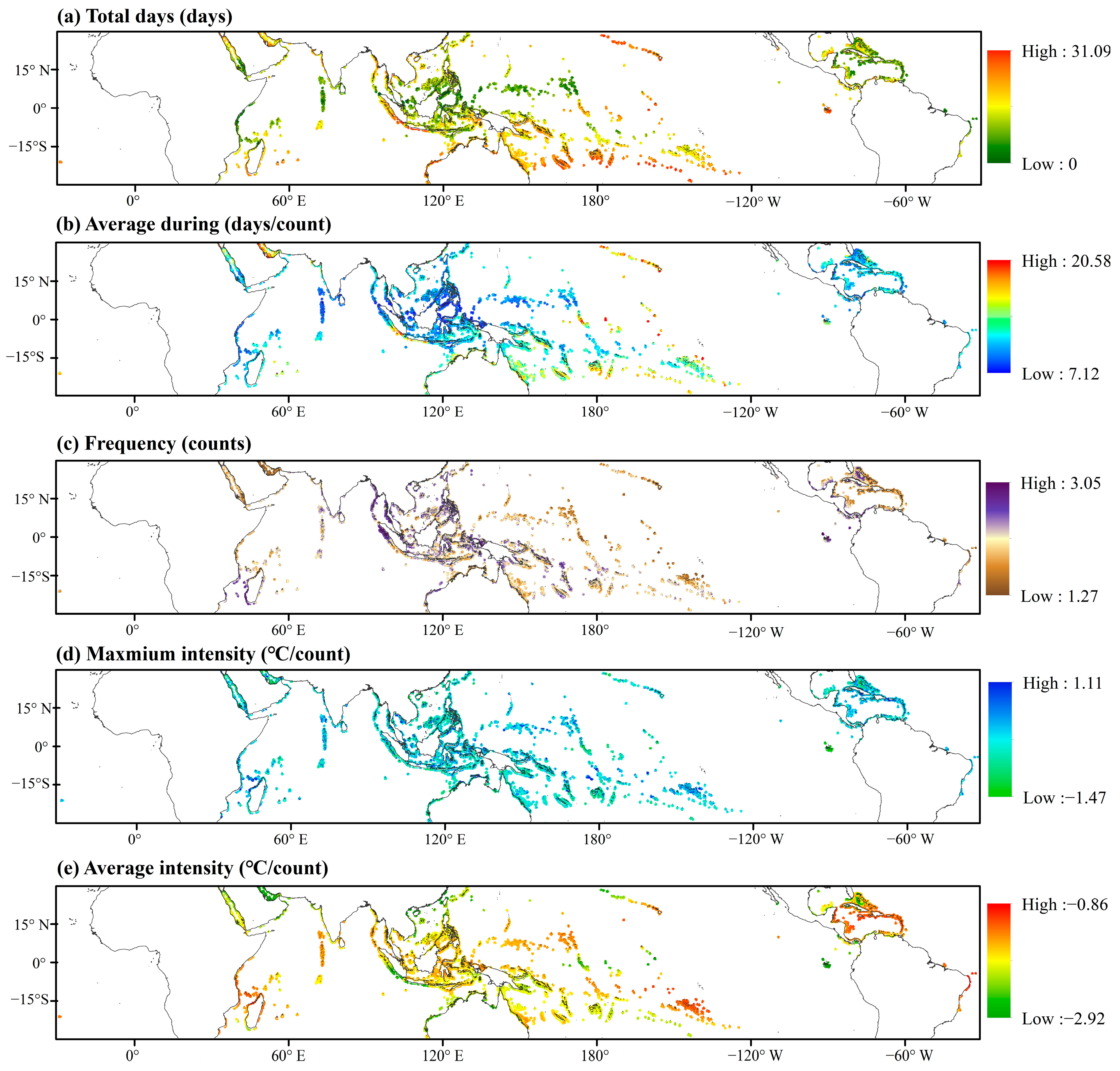
As illustrated in Figure 3 and Figure 4, the spatiotemporal distribution patterns in MHWs and MCSs show significant spatial heterogeneity. In general, MHWs in higher-latitude coral reef zones are characterized by longer durations and higher intensity, with up to 1.24 times more MHW days than equatorial regions (

Table A3. Trend and significance of MHW indicators within latitude bands.

Total Days	30° N–15° N	15° N–0°	0° N–15° S	15° S–30° S
trend	1.309	1.051	1.135	1.241
p-value	0.000	0.000	0.000	0.000
Average Duration
trend	0.196	0.148	0.193	0.213
p-value	0.000	0.000	0.000	0.000
Frequency
trend	0.080	0.069	0.056	0.057
p-value	0.000	0.000	0.000	0.000
Max Intensity
trend	0.006	−0.002	−0.002	0.006
p-value	0.000	0.444	0.347	0.002

and

Table A4. Trend and significance of MCS indicators within latitude bands.

Total Days	30° N–15° N	15° N–0°	0° N–15° S	15° S–30° S
trend	−0.929	−0.951	−1.038	−1.005
p-value	0.000	0.000	0.000	0.000
Average Duration
trend	−0.031	−0.034	−0.012	−0.043
p-value	0.280	0.022	0.579	0.175
Frequency
trend	−0.081	−0.096	−0.102	−0.077
p-value	0.000	0.000	0.000	0.000
Max Intensity
trend	−0.009	−0.007	−0.006	−0.004
p-value	0.000	0.000	0.000	0.000

and Figure A1). The spatial distribution of MCS frequency is similar to that of MHWs but features shorter durations and contrasting trends in average intensity.

Specifically, the total days of both MHWs and MCSs (the sum of all days of MHWs/MCSs per year) vary significantly across regions (Figure 3a and Figure 4a). High figures for total days are observed in regions like the Red Sea, the Persian Gulf, the Hawaiian Islands, the Galapagos Islands, the South Pacific Islands, coastal Australia, and the southwestern coast of Sumatra, with MHWs reaching up to 32 days and MCSs reaching up to 31 days. In contrast, lower numbers of total days are observed in regions like eastern Africa, northern Madagascar, equatorial areas, and the Caribbean Sea.

The average duration of MHWs and MCSs (the average duration of MHW/MCS events per year) also varies across coral reef zones (Figure 3b and Figure 4b). Most regions experience MHWs lasting fewer than 20 days/count and MCSs lasting fewer than 10 days/count. However, in some regions, the longest average duration of MHWs can extend up to 31 days/count, while MCSs can reach up to 20 days/count.

Regarding the frequency of MHWs and MCSs (the total counts of MHW/MCS events per year, Figure 3c and Figure 4c), high-frequency MHWs primarily occur in East Asia, northern Australia, southern Madagascar, and the southern peninsula of Florida, where events occur several times per year on average. These regions, located near continents or at higher latitudes, experience multiple events per year on average. Similarly, high-frequency MCSs occur in western Madagascar, East Asia, northern Australia, and the Galapagos Islands, with frequencies approaching three times per year. Conversely, low-frequency regions of both MHWs and MCSs are identified in the Pacific Ocean, the Red Sea, the Persian Gulf, and the Caribbean Sea.

Regions with a high maximum intensity of MHWs (the maximum intensity of SST anomalies during MHW/MCS events per year, Figure 3d and Figure 4d) are typically located in high-latitude coral reef zones, whereas low-intensity areas are found in equatorial oceans. For MCS, most coral reef zones exhibit a high maximum intensity, with low-intensity areas mainly found in the Galapagos Islands, the South Pacific Islands, southwestern Sumatra, and northwestern Australia. The spatial distribution patterns of average intensity for both MHWs and MCSs (the average intensity of SST anomalies during MHW/MCS events per year, Figure 3e and Figure 4e) closely follow those of maximum intensity.

3.2. Global Trends in Mean MHW and MCS Metrics in Coral Reef Zones from 1982 to 2022

From 1982 to 2022, MHW events have increased, while MCS events have decreased, exhibiting significant spatial heterogeneity across the entire coral reef regions, particularly in East Asia, the South Pacific, and the Caribbean (Figure 5 and Figure 6). MHW total days have increased substantially in most regions, particularly in the Red Sea, the northern Persian Gulf, and the South Pacific islands, with rates of up to 28 days/decade. Additionally, the average duration of MHW events has increased by 1–2 days/event/decade, while the frequency has increased by 1–1.9 events/decade, especially in the Red Sea, the Persian Gulf, eastern East Asia, and the South Pacific islands.

MHW events in global coral reef regions have become more extreme over time (Figure 7g,i). Specifically, the average intensity of MHWs has decreased by 0.1 °C/count/decade, while the maximum intensity has increased by 0.1 °C/count/decade. Additionally, the average intensity tends to be higher during strong El Niño years.

Conversely, as shown in Figure 7, the MCS total days have decreased by approximately 10.5 days/decade, with a similar reduction in average duration by 0–5 days/count/decade across most coral reef areas. The frequency of MCS events has also decreased by 0.9–2.4 counts/decade. However, the maximum intensity of MCSs has increased in coral reef regions between 15° and 30° latitude north and south at a rate of 0–0.1 °C/count/decade. Despite this overall decline, the maximum intensity of MCSs continues to show variability, as illustrated by the quadratic trend fitted to the MCS mean intensity variable (Figure 7j).

3.3. Global Trends in Mean MHW and MCS Metrics in Coral Reef Zones from 2023 to 2070

The projections suggest a significant increase in MHW duration, frequency, and intensity in the future, particularly under the SSP5–8.5 scenario in the Marshall Islands and the Caribbean Sea regions, while MCS events are expected to decrease in both frequency and intensity across most coral reef regions, particular in the South Pacific.

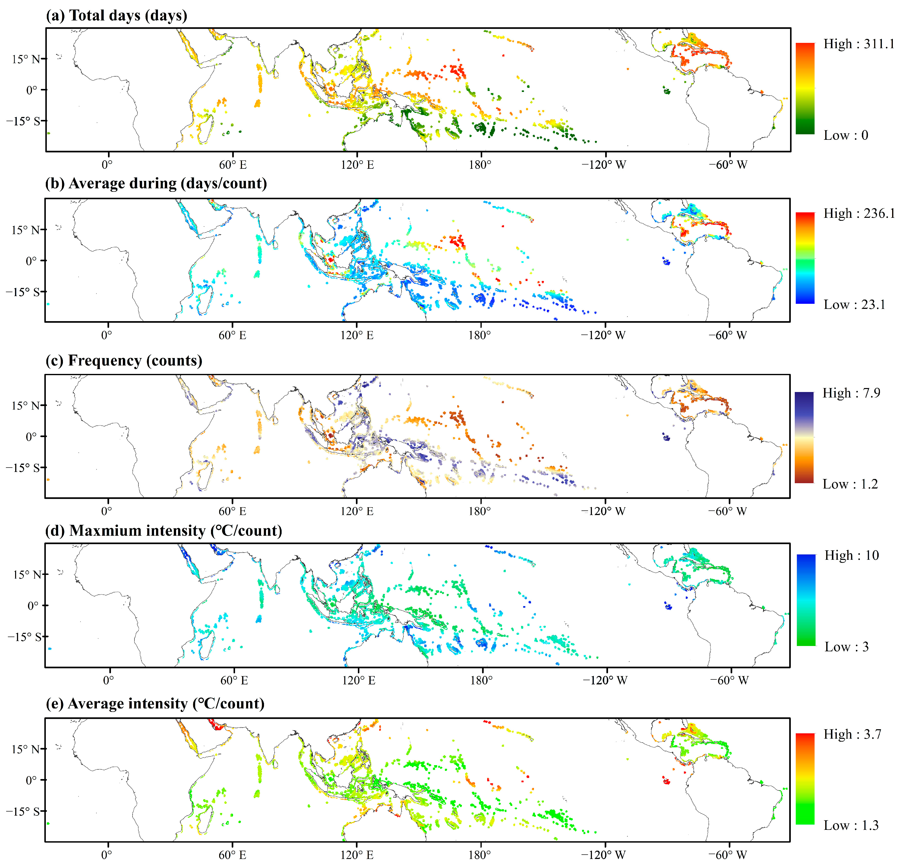
Under the SSP2–4.5 scenario, the results for MHWs showed that the total days of MHWs exceeded 150 days in most coral reef regions, with the eastern part of Indonesia, the Marshall Islands, and the Caribbean Sea approaching 300 days (Figure 8). The average annual duration of MHWs ranged from 14 to 170 days/count, with the aforementioned regions experiencing durations exceeding 120 days. The frequency of MHWs was particularly high in the Indo-Pacific and Caribbean regions, approaching eight counts per year. The average warming intensity of MHWs varied between 1 °C and 3 °C/count, with the maximum intensity reaching up to 8 °C, primarily observed in the Persian Gulf.

When comparing the SSP5–8.5 scenario to the SSP2–4.5 scenario, all five MHW metrics showed an increasing trend under the SSP5–8.5 scenario (Figure 9). The main hotspot regions for MHWs under this scenario were the central–western Pacific and the Caribbean Sea, where both the total duration and intensity of MHW events were projected to intensify further. Furthermore, a summary of the total MHW days under the SSP5–8.5 scenario revealed that regions experiencing more than 200 MHW days per year would encompass over 70% of the area by 2070. As a result, MHWs are projected to become nearly year-round by 2070 under scenario SSP5–8.5.

Regarding MCS, under the SSP2–4.5 scenario, the total number of days of MCSs in most coral reef areas was less than 4 days, and the average duration of MCSs was typically less than 10 days/count. The frequency of MCS events was low, with the maximum intensity of MCSs being weak, ranging from −3 °C to −1 °C/count, especially in the South Pacific region (Figure 10).

Under the SSP5–8.5 scenario (Figure 11), the total number of days of MCS events was projected to decrease further, with even shorter average durations and lower frequencies. The intensity of MCS events also weakened under this scenario, particularly in the South Pacific, where the maximum intensity was significantly lower compared to other regions.

Between 1982 and 2022, the area affected by MHWs was less than 20 times the size of the area impacted by MCSs. However, under future global warming scenarios, SSTs in coral reef zones are expected to increase at a rate of 0.2–0.3 °C per decade. In addition, the area ratio between MHWs and MCSs is projected to continue increasing significantly. By 2070, under the SSP2–4.5 scenario, this ratio is expected to reach a maximum of approximately 100 times, and under the more extreme SSP5–8.5 scenario, it could rise by as many as 196 times, especially after 2040 (Figure 12). As a result, MHWs are projected to dominate coral reef zones in the future, particularly under the SSP5–8.5 scenario.

3.4. The Underlying Factors Shaping the Spatial Heterogeneity of MHWs

Figure 13 shows that only 13 features were retained, effectively mitigating the risk of overfitting. The models performed well, with all R² values around 0.9 (Figure A2). While the importance ranking of features varied across the four models, a consistent trend emerged. In all models, t2m_a_cv (annual coefficient of variation of 2 m air temperature) was consistently ranked as the most important feature. The second and third most important features differed slightly across models. For the sake of simplicity and consistency, these features have been consolidated into the top three most influential factors, which are t2m_a_cv, OHC_a_cv (annual coefficient of variation in ocean heat content), and t2m_m_cv (monthly coefficient of variation of 2 m air temperature). As these factors increased, the number of MHW total days correspondingly rose. Furthermore, the coefficient of variation (CV) exerted a stronger influence than mean values, encompassing both interannual and intra-annual (month-to-month) CVs of temperature.

3.5. Relationship Between MHWs/MCSs and Coral Coverage

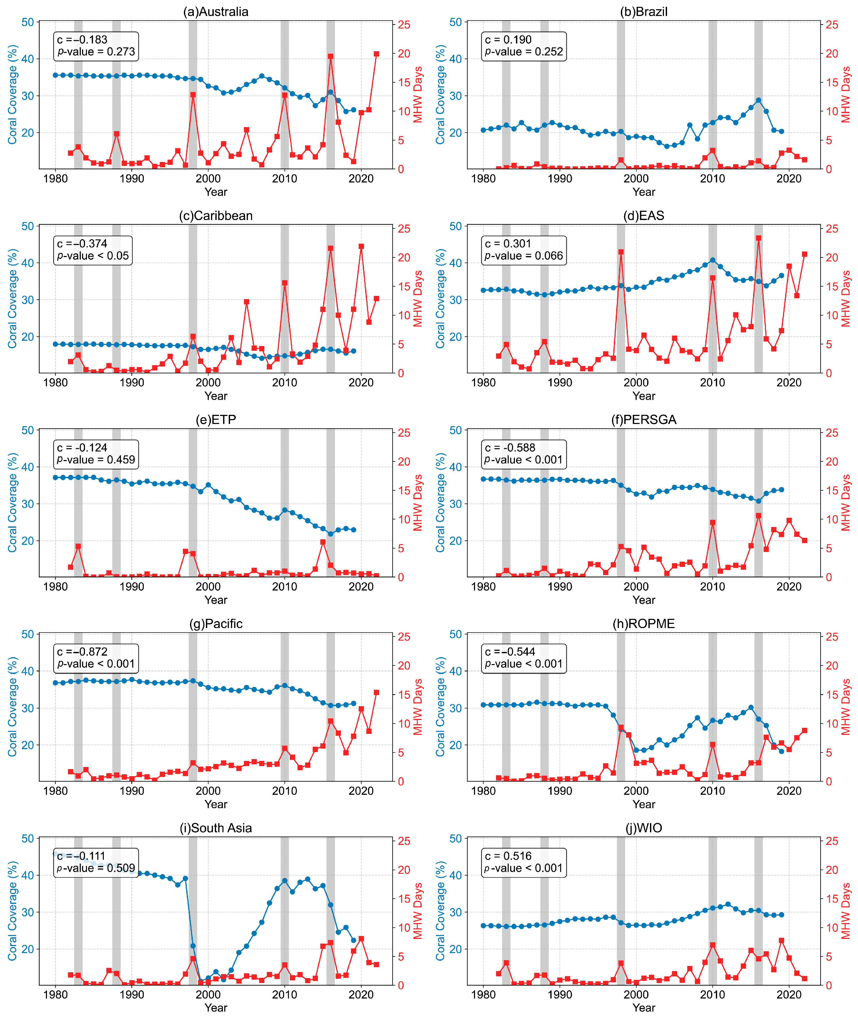
Figure 14 demonstrates an inverse relationship between coral coverage and MHWs (c = −0.54, p < 0.01) while showing a significant positive correlation with MCSs (c = 0.6, p < 0.01). Specifically, around 1998, 2010, and 2016, high MHW values corresponded to declining coral coverage. Despite a rapid decline in MHWs after 1998, coral coverage continued to decline, reaching 30% by 2001 and demonstrating post-mortality processes. Coral coverage continued to increase from 2001, until severe MHWs began in 2008. Due to the increasing frequency, intensity, and duration of MHWs, coral cover has exhibited a downward trend, with only a slight recovery observed in 2018.

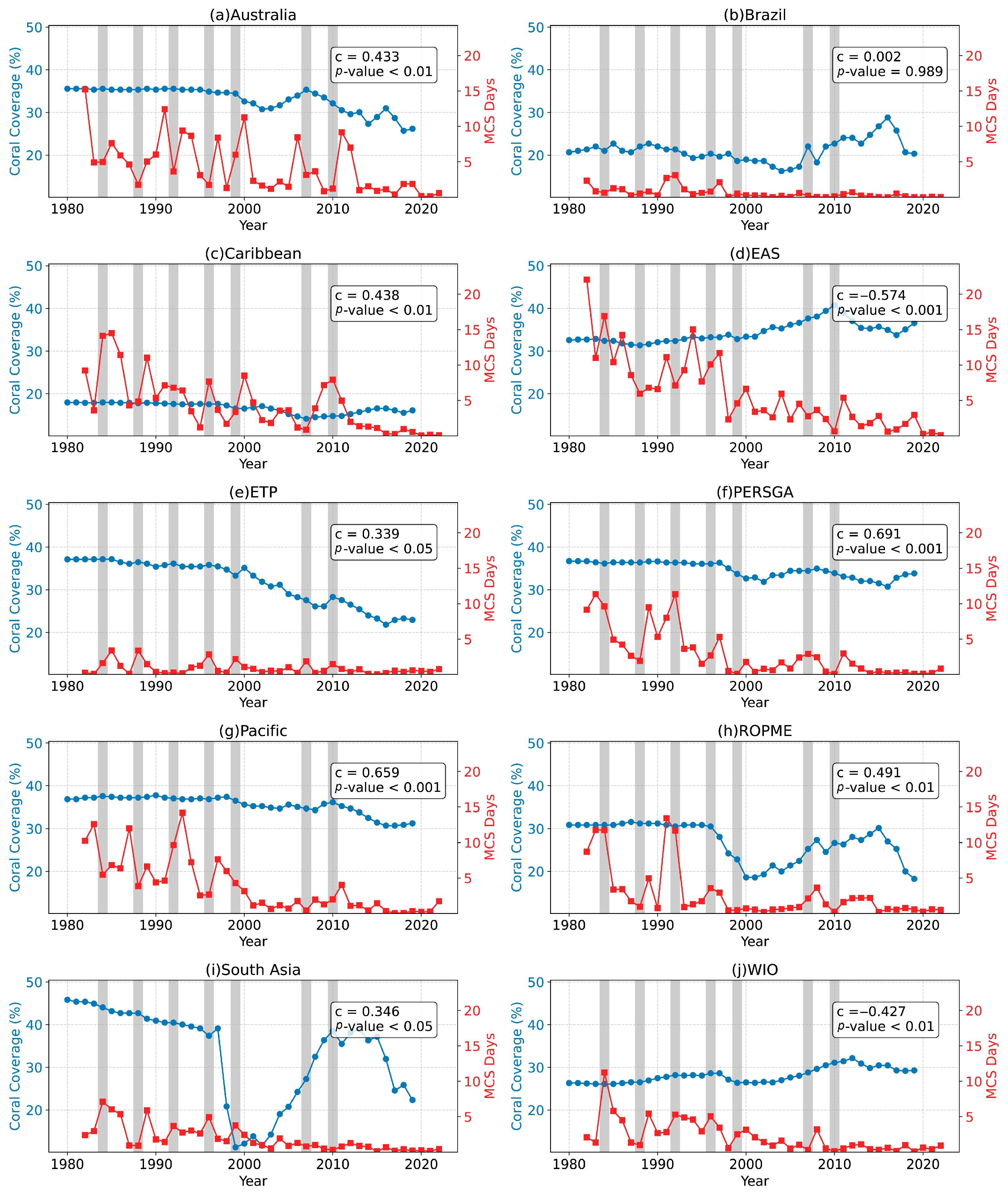
From the perspective of different coral reef regions (Figure A3), the Pacific region shows the strongest negative correlation (c = −0.87, p < 0.001), followed by PERSGA (c = −0.59, p < 0.001), ROPME (c = −0.54, p < 0.001), and WIO (c = −0.52, p < 0.001). In contrast, MCSs and coral reef cover both exhibits decreasing trends, resulting in a positive correlation (Figure A4).

4. Discussion

4.1. Higher-Latitude Coral Reefs Are Experiencing More Severe MHWs than Equatorial Regions

Our findings reveal that MHW intensity is higher in lower-temperature regions. This implies that coral reefs at higher latitudes endure more intense MHWs compared to their equatorial counterparts (Table A3 and Table A4 and Figure A1). Multiple factors may account for this warming asymmetry, as follows. (i) Greater seasonal SST variability (Figure 15a) and warming trends (Figure 15b) at higher latitudes may result in anomalies that more frequently exceed a fixed threshold. (ii) In higher-latitude coral reef areas, atmospheric conditions, such as high-pressure systems, may reduce cloud cover, thereby increasing solar radiation. This, in turn, enhances surface water temperature and stratification differences, promoting the development of MHWs [47]. (iii) Some physical oceanographic mechanisms could shape this pattern. For example, a study in the Northwestern South China Sea suggests that wind weakening and enhanced stratification can inhibit upwelling, which in turn favors the development of MHWs [48]. (iv) The subtropical regions generally exhibit lower baseline temperatures relative to equatorial zones. This temperature gradient enables subtropical regions to absorb heat more efficiently. Coupled with elevated solar radiation, these conditions render subtropical regions especially vulnerable to MHW events [49].

Intense MHWs in higher-latitude regions threaten their potential as coral refuges—areas theorized to shelter coral species during global warming due to their naturally cooler temperatures [50]. What is worse, these regions are frequently subject to intense human activities, which may reduce live coral cover and degrade reef communities, thereby heightening the susceptibility of corals in higher-latitude waters to extreme climatic events [51].

4.2. Upper-Ocean Warming Is One of the Most Important Drivers of the Trends in MHWs and MCSs

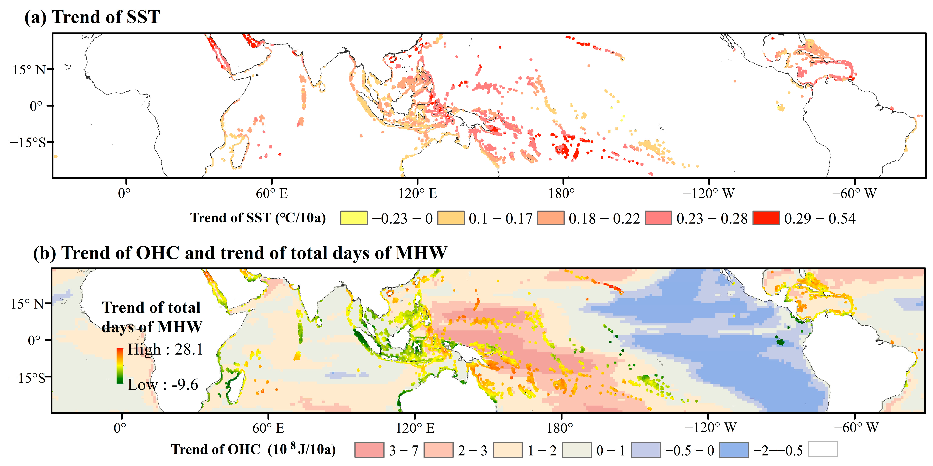
Four machine learning approaches demonstrate that ocean heat content (OHC) is one of the primary drivers of MHWs. To elucidate spatial variations in OHC, we compared the multi-year linear trend of OHC at depths of 0–300 m with the spatial distribution of MHWs (Figure 16). The increase in OHC and SST corresponds to the areas where MHW days have increased. Specifically, SST shows an upward trend across the entire coral reef region, especially in the northern Indian Ocean, eastern East Asia, South Pacific islands, and the North Atlantic. In these regions, OHC is also increasing. This pattern aligns with the distribution of coral reefs, which are primarily located in regions with rising OHC.

Higher ocean heat content (0–300 m) can indicate a larger subsurface heat reservoir and increased stratification, which make the surface more susceptible to extremes [52,53]. Prior research has similarly established that SST warming predominantly drives increases in the duration and frequency of MHWs [16]. Additionally, high interannual variability suggests a greater likelihood of extreme deviations [54,55].

We also observed that strong El Niño years are associated with MHWs. The impact of ENSO is primarily evident in the tropical Pacific, the tropical Indian Ocean, and regions like the Great Barrier Reef in Australia [23]. SST anomalies in the tropical eastern Pacific can strengthen the downward branch of the tropical Walker circulation in the western Indian Ocean, leading to more frequent MHWs in areas where coral reefs are concentrated [56]. Furthermore, ENSO can increase the frequency and intensity of MHWs by stimulating warm atmospheric Rossby waves [26]. The influence of the Indian Ocean Dipole (IOD) on the interannual variation in MHWs is mainly observed in the tropical Indian Ocean and the tropical Pacific [23]. For example, negative IOD events cause the thermocline to deepen, weakening the upwelling of cold waters along the coast and thereby promoting the occurrence of MHWs [57].

4.3. MHWs Are Projected to Continue Increasing in the Future

Under future warming, events are measured against present-day thresholds, resulting in the projection of nearly year-round MHWs by 2070. Oliver et al. [58] similarly noted that the frequency and duration of MHWs have risen, driving a 54% increase in global annual MHW days, with the most pronounced increases observed in the high-latitude North Atlantic. Under the SSP5–8.5 scenario, intensified global warming is projected to markedly increase the MHW-to-MCS area ratio, underscoring the pivotal role of warming magnitude in shaping future MHW and MCS dynamics. According to Hughes et al. [4], the extensive 2016 damage coupled with continuing temperature increases make the recovery of the northern Great Barrier Reef to its original status unlikely, with projections indicating that a fourth mass bleaching episode is probable within the next 10–20 years.

Forecasting MHWs is increasingly vital for safeguarding coral reef ecosystems. Our findings reveal that the coefficient of variation (CV), rather than the mean, exerts the strongest influence on MHW intensity. This stems primarily from MHW intensity reflecting the extent of SST deviation from its historical mean, with the CV of 2 m air temperature similarly capturing such variability. Consequently, the CV of air temperature and OHC has emerged as the most critical determinant. Accordingly, we underscore that future MHW predictions should prioritize the CV of predictive indicators over reliance on mean values alone. However, numerous studies have overlooked these factors [59,60,61,62].

4.4. Relationship Between MHWs/MCSs and Coral Coverage

MHWs have both direct and indirect effects that may lead to post-mortality processes in coral reefs. (i) Coral bleaching caused by symbiotic algae expulsion leads to coral mortality [63]. (ii) Phototrophic microbes lead to the rapid microbial bioerosion of coral skeletons, and this process is exacerbated by the nitrogen released from dead corals and high temperatures [64,65]. (iii) Competitive algae occupy the habitat, attracting excavating fish herbivores, further promoting bioerosion, and leading to coral larval recruitment failure [66,67], as well as suppressing algal competition [68]. Therefore, the destruction caused by MHWs to both the biological community and physical structure reduces the ecosystem’s structural complexity [69]. Coral death can still occur after severe MHW events.

The observed lag effects of recovery can be attributed to several interacting factors, including a limited larval supply [67,70,71], thermally tolerant symbionts reducing the growth of their coral hosts [66], shifts toward coral–algal dominance [72], and the cumulative impact of sequential disturbances, such as disease and ocean acidification [73,74].

We found that the decrease in MCS days and the reduction in coral coverage showed a significant positive relationship, which can be explained as follows. (i) The increase in MHWs is often accompanied by a decrease in MCSs, and the reduction in coral coverage is dominated by the positive correlation with MHW [20,75]. However, MCSs may still provide a window for coral to recover from heat stress [76]. (ii) Decreased cold spells may lead to reduced upwelling, thereby reducing nutrient supply and affecting coral health and recovery capacity [77]. Therefore, we emphasize that future research should focus not only on heatwaves but also on developing the study of cold spells.

4.5. Implications

In response to increasingly severe global warming, previous research has proposed various potential responses in coral reefs, including migration to refuges in high-latitude regions [78,79,80]. Our research asserts that high-latitude coral reefs are experiencing more intense MHWs and MCSs compared to equatorial regions, underscoring the need to prioritize the protection of coral refuges. Additionally, the coral reefs in the Pacific and Caribbean regions, where the intensity of MHWs is gradually increasing, should be given more attention.

Coral reef recovery exhibits a lag effect, meaning that even after a reduction in MHWs, recovery remains slow, showing a post-mortality process. This has emphasized the need for long-term protection and restoration efforts rather than reactive measures during extreme weather events. Integrating the establishment of protected areas and long-term strategies, such as ecological restoration, into climate change mitigation efforts is crucial for ensuring the sustained health of coral reef ecosystems.

4.6. Limitations and Prospects

Firstly, the selection of projection models primarily considers spatial resolution. Given that three models represent a relatively small ensemble, it is important to acknowledge that while they may provide an initial projection, they may not capture the full uncertainty range of CMIP6 outcomes. Further studies should utilize a larger ensemble of regionally downscaled data to reduce model uncertainty. Secondly, the baseline assumptions in the study are static, meaning that the research does not account for the adaptability of coral reefs. Corals are likely to experience conditions far outside of their historical norms in the next 50 years. The next step should involve considering multiple baseline scenarios to compare and analyze the spatial and temporal patterns of future marine heatwaves in coral reef areas, which could provide more robust results [81]. Thirdly, although the correlations between MHWs/MCSs and coral cover offer valuable insights into the relationship between these factors and coral dynamics, such relationships may not be easily captured through simple linear assumptions. Future studies should incorporate these indicators into lagged regression models or structural equation modeling to more effectively identify the key drivers of coral bleaching and mortality [82]. In addition, determining the top three factors in the four machine learning models, treated as equally important, should be further investigated. For example, Ensemble Learning techniques, such as Bagging, Boosting, or Stacking, could combine multiple learners (such as the four models we used) to reduce variance and bias while improving prediction accuracy, ultimately yielding a unified result [83].

5. Conclusions

In this study, we utilized daily SST data from 1982 to 2070 to explicitly depict the spatiotemporal patterns and trends of MHWs and MCSs. Additionally, we applied four machine learning models to investigate the driving mechanisms of MHW intensity. At last, we explored the relationship between coral coverage and MHWs/MCSs. The conclusions and implications are as follows:

(1)

Over the last four decades, MHWs have not only been increasing in average intensity but also becoming more extreme, while MCSs have declined. The Red Sea, the Persian Gulf, the Hawaiian Islands, the Galapagos Islands, the South Pacific Islands, coastal Australia, and southwestern Sumatra experience high numbers of total days of MHWs, reaching up to 32 days, and MCSs for up to 31 days. The average total days of MHWs are increasing at a rate of up to 28 days/decade.

(2)

Higher-latitude coral reefs face more severe MHWs than their equatorial counterparts, with up to 1.24 times more MHW days, highlighting the need to prioritize the protection of coral refuges in these vulnerable regions.

(3)

The coefficient of variation (CV) of annual temperature, the annual ocean heat content, and the monthly temperature were important factors driving MHW intensity. We emphasize the critical role of climate variability (CV) over mean climate as a major driver of MHW and further highlight that future MHW predictions should focus more on the CV of forecasting indicators rather than just the climate means to provide new insights for future projections.

(4)

From 2023 to 2070, the SST in coral reef zones is projected to rise by 0.2–0.3 °C per decade. We highlight that MHWs are expected to occur nearly year-round under scenario SSP5–8.5, while MCSs are anticipated to decline sharply. The MHW-to-MCS area ratio is forecasted to surge after 2040, reaching approximately 100 times under SSP2–4.5 and 196 times under SSP5–8.5 by 2070, particularly in the Marshall Islands and the Caribbean Sea.

(5)

Coral coverage shows a strong negative correlation with MHW intensity (r = −0.54, p < 0.01) and a significant positive correlation with MCSs (r = 0.6, p < 0.01). Coral coverage in the Pacific region demonstrates the highest sensitivity to MHWs. Globally, it shows a recovery lag and post-mortality processes following MHWs.

References

1. Hobday, A.J.; Alexander, L.V.; Perkins, S.E.; Smale, D.A.; Straub, S.C.; Oliver, E.C.; Benthuysen, J.A.; Burrows, M.T.; Donat, M.G.; Feng, M.; et al. A Hierarchical Approach to Defining Marine Heatwaves. Prog. Oceanogr. 2016, 141, 227–238. [Google Scholar] [CrossRef]
2. Hoegh-Guldberg, O.; Mumby, P.J.; Hooten, A.J.; Steneck, R.S.; Greenfield, P.; Gomez, E.; Harvell, C.D.; Sale, P.F.; Edwards, A.J.; Caldeira, K.; et al. Coral Reefs under Rapid Climate Change and Ocean Acidification. Science 2007, 318, 1737–1742. [Google Scholar] [CrossRef]
3. Pan, Y.; Sun, W.; Bao, S.; Xie, M.; Jiang, L.; Ji, J.; Yu, Y.; Dong, C. Global Variability and Future Projections of Marine Heatwave Onset and Decline Rates. Remote Sens. 2025, 17, 1362. [Google Scholar] [CrossRef]
4. Hughes, T.P.; Kerry, J.T.; Álvarez-Noriega, M.; Álvarez-Romero, J.G.; Anderson, K.D.; Baird, A.H.; Babcock, R.C.; Beger, M.; Bellwood, D.R.; Berkelmans, R.; et al. Global Warming and Recurrent Mass Bleaching of Corals. Nature 2017, 543, 373–377. [Google Scholar] [CrossRef]
5. Yao, Y.; Wang, J.; Yin, J.; Zou, X. Marine Heatwaves in China’s Marginal Seas and Adjacent Offshore Waters: Past, Present, and Future. J. Geophys. Res. Oceans 2020, 125, e2019JC015801. [Google Scholar] [CrossRef]
6. Yu, X.; Yu, K.; Chen, B.; Liao, Z.; Liang, J.; Yao, Q.; Qin, Z.; Wang, H.; Yu, J. Different Responses of Scleractinian Coral Acropora pruinosa from Weizhou Island during Extreme High Temperature Events. Coral Reefs 2021, 40, 1697–1711. [Google Scholar] [CrossRef]
7. Pandolfi, J.M.; Connolly, S.R.; Marshall, D.J.; Cohen, A.L. Projecting Coral Reef Futures under Global Warming and Ocean Acidification. Science 2011, 333, 418–422. [Google Scholar] [CrossRef] [PubMed]
8. Gardner, T.A.; Côté, I.M.; Gill, J.A.; Grant, A.; Watkinson, A.R. Long-Term Region-Wide Declines in Caribbean Corals. Science 2003, 301, 958–960. [Google Scholar] [CrossRef] [PubMed]
9. Brodie, J.; Waterhouse, J. A Critical Review of Environmental Management of the ‘Not so Great’Barrier Reef. Estuar. Coast. Shelf Sci. 2012, 104, 1–22. [Google Scholar] [CrossRef]
10. Birkeland, C. Coral Reefs in the Anthropocene; Springer: Berlin/Heidelberg, Germany, 2015. [Google Scholar]
11. Hughes, T.P.; Kerry, J.T.; Baird, A.H.; Connolly, S.R.; Dietzel, A.; Eakin, C.M.; Heron, S.F.; Hoey, A.S.; Hoogenboom, M.O.; Liu, G.; et al. Global Warming Transforms Coral Reef Assemblages. Nature 2018, 556, 492–496. [Google Scholar] [CrossRef] [PubMed]
12. Maynard, J.A.; Turner, P.J.; Anthony, K.R.; Baird, A.H.; Berkelmans, R.; Eakin, C.M.; Johnson, J.; Marshall, P.A.; Packer, G.R.; Rea, A.; et al. ReefTemp: An Interactive Monitoring System for Coral Bleaching Using High-Resolution SST and Improved Stress Predictors. Geophys. Res. Lett. 2008, 35. [Google Scholar] [CrossRef]
13. Feng, Y.; Bethel, B.J.; Dong, C.; Zhao, H.; Yao, Y.; Yu, Y. Marine Heatwave Events near Weizhou Island, Beibu Gulf in 2020 and Their Possible Relations to Coral Bleaching. Sci. Total Environ. 2022, 823, 153414. [Google Scholar] [CrossRef]
14. Van Woesik, R.; Houk, P.; Isechal, A.L.; Idechong, J.W.; Victor, S.; Golbuu, Y. Climate-Change Refugia in the Sheltered Bays of P Alau: Analogs of Future Reefs. Ecol. Evol. 2012, 2, 2474–2484. [Google Scholar] [CrossRef] [PubMed]
15. Schlegel, R.W.; Oliver, E.C.; Perkins-Kirkpatrick, S.; Kruger, A.; Smit, A.J. Predominant Atmospheric and Oceanic Patterns during Coastal Marine Heatwaves. Front. Mar. Sci. 2017, 4, 323. [Google Scholar] [CrossRef]
16. Oliver, E.C.; Donat, M.G.; Burrows, M.T.; Moore, P.J.; Smale, D.A.; Alexander, L.V.; Benthuysen, J.A.; Feng, M.; Sen Gupta, A.; Hobday, A.J.; et al. Longer and More Frequent Marine Heatwaves over the Past Century. Nat. Commun. 2018, 9, 1324. [Google Scholar] [CrossRef] [PubMed]
17. Tan, H.; Cai, R.; Yan, X.; Li, C. Amplification of Winter Sea Surface Temperature Response over East China Seas to Global Warming Acceleration and Slowdown. Int. J. Climatol. 2021, 41, 2082–2099. [Google Scholar] [CrossRef]
18. Ren, J.; Wang, C.; Yao, Y. Spatiotemporally Continuous Marine Heatwaves: A Novel Clustering Approach Reveals Increasing Frequency, Duration, Area, Intensity, and Movement Distance. Geophys. Res. Lett. 2025, 52, e2024GL113211. [Google Scholar] [CrossRef]
19. Amaya, D.J.; Miller, A.J.; Xie, S.-P.; Kosaka, Y. Physical Drivers of the Summer 2019 North Pacific Marine Heatwave. Nat. Commun. 2020, 11, 1903. [Google Scholar] [CrossRef]
20. Sun, W.; Wang, Y.; Yang, Y.; Yang, J.; Ji, J.; Dong, C. Marine Heatwaves/cold spells Associated with Mixed Layer Depth Variation Globally. Geophys. Res. Lett. 2024, 51, e2024GL112325. [Google Scholar] [CrossRef]
21. Zhang, W.; Zheng, Z.; Zhang, T.; Chen, T. Strengthened Marine Heatwaves over the Beibu Gulf Coral Reef Regions from 1960 to 2017. Haiyang Xuebao 2020, 42, 45–52. [Google Scholar]
22. Qiao, L.; Tang, H.; Huang, G. Drivers and Predictability of Summer Marine Heatwaves in the Northwest Pacific. J. Geophys. Res. Atmospheres 2025, 130, e2024JD042994. [Google Scholar] [CrossRef]
23. Holbrook, N.J.; Scannell, H.A.; Sen Gupta, A.; Benthuysen, J.A.; Feng, M.; Oliver, E.C.; Alexander, L.V.; Burrows, M.T.; Donat, M.G.; Hobday, A.J.; et al. A Global Assessment of Marine Heatwaves and Their Drivers. Nat. Commun. 2019, 10, 2624. [Google Scholar] [CrossRef]
24. Scannell, H.A.; Pershing, A.J.; Alexander, M.A.; Thomas, A.C.; Mills, K.E. Frequency of Marine Heatwaves in the North Atlantic and North Pacific since 1950. Geophys. Res. Lett. 2016, 43, 2069–2076. [Google Scholar] [CrossRef]
25. England, M.H.; Li, Z.; Huguenin, M.F.; Kiss, A.E.; Sen Gupta, A.; Holmes, R.M.; Rahmstorf, S. Drivers of the Extreme North Atlantic Marine Heatwave during 2023. Nature 2025, 642, 636–643. [Google Scholar] [CrossRef]
26. Di Lorenzo, E.; Mantua, N. Multi-Year Persistence of the 2014/15 North Pacific Marine Heatwave. Nat. Clim. Change 2016, 6, 1042–1047. [Google Scholar] [CrossRef]
27. Li, Z.; Holbrook, N.J.; Zhang, X.; Oliver, E.C.; Cougnon, E.A. Remote Forcing of Tasman Sea Marine Heatwaves. J. Clim. 2020, 33, 5337–5354. [Google Scholar] [CrossRef]
28. Zhang, Y.; Du, Y.; Feng, M.; Hu, S. Long-Lasting Marine Heatwaves Instigated by Ocean Planetary Waves in the Tropical Indian Ocean during 2015–2016 and 2019–2020. Geophys. Res. Lett. 2021, 48, e2021GL095350. [Google Scholar] [CrossRef]
29. Schlegel, R.W.; Oliver, E.C.; Wernberg, T.; Smit, A.J. Nearshore and Offshore Co-Occurrence of Marine Heatwaves and cold spells. Prog. Oceanogr. 2017, 151, 189–205. [Google Scholar] [CrossRef]
30. Schlegel, R.W.; Darmaraki, S.; Benthuysen, J.A.; Filbee-Dexter, K.; Oliver, E.C. Marine cold spells. Prog. Oceanogr. 2021, 198, 102684. [Google Scholar] [CrossRef]
31. Yao, Y.; Wang, C.; Fu, Y. Global Marine Heatwaves and cold spells in Present Climate to Future Projections. Earths Future 2022, 10, e2022EF002787. [Google Scholar] [CrossRef]
32. Li, C.; Sun, W.; Ji, J.; Zhu, Y. Historical Marine Cold Spells in the South China Sea: Characteristics and Trends. Remote Sens. 2024, 16, 1171. [Google Scholar] [CrossRef]
33. Rich, W.A.; Carvalho, S.; Berumen, M.L. Coral Bleaching Due to Cold Stress on a Central Red Sea Reef Flat. Ecol. Evol. 2022, 12, e9450. [Google Scholar] [CrossRef] [PubMed]
34. Yu, K.-F.; Zhao, J.-X.; Liu, T.-S.; Wei, G.-J.; Wang, P.-X.; Collerson, K.D. High-Frequency Winter Cooling and Reef Coral Mortality during the Holocene Climatic Optimum. Earth Planet. Sci. Lett. 2004, 224, 143–155. [Google Scholar] [CrossRef]
35. Dinesh, A.S.; Kumar, P.; Mishra, A.K.; Pandey, L.K.; Tewari, M.; Cabos, W.; Sein, D.V. Analyzing Future Marine Cold Spells in the Tropical Indian Ocean: Insights from a Regional Earth System Model. Q. J. R. Meteorol. Soc. 2024, 150, 1668–1685. [Google Scholar] [CrossRef]
36. Frölicher, T.L.; Fischer, E.M.; Gruber, N. Marine Heatwaves under Global Warming. Nature 2018, 560, 360–364. [Google Scholar] [CrossRef]
37. Souter, D.; Planes, S.; Wicquart, J.; Logan, M.; Obura, D.; Staub, F. Status of Coral Reefs of the World: 2020: Executive Summary. 2021. Available online: https://bvearmb.do/handle/123456789/3190 (accessed on 27 November 2023).
38. Souter, D.; Planes, S.; Wicquart, J.; Logan, M.; Obura, D.; Staub, F. Status of Coral Reefs of the World: 2020: Summary for Policymakers. 2021. Available online: https://bvearmb.do/handle/123456789/3191 (accessed on 27 November 2023).
39. Wang, Y.; Zhou, Y. Seasonal Dynamics of Global Marine Heatwaves over the Last Four Decades. Front. Mar. Sci. 2024, 11, 1406416. [Google Scholar] [CrossRef]
40. Oliver, E.C.; Benthuysen, J.A.; Darmaraki, S.; Donat, M.G.; Hobday, A.J.; Holbrook, N.J.; Schlegel, R.W.; Sen Gupta, A. Marine Heatwaves. Annu. Rev. Mar. Sci. 2021, 13, 313–342. [Google Scholar] [CrossRef]
41. Babcock, R.; Thomson, D.; Haywood, M.; Vanderklift, M.; Pillans, R.; Rochester, W.; Miller, M.; Speed, C.; Shedrawi, G.; Field, S.; et al. Recurrent Coral Bleaching in North-Western Australia and Associated Declines in Coral Cover. Mar. Freshw. Res. 2020, 72, 620–632. [Google Scholar] [CrossRef]
42. Li, Y.; Ren, G.; Wang, Q.; Mu, L. Changes in Marine Hot and Cold Extremes in the China Seas during 1982–2020. Weather Clim. Extrem. 2023, 39, 100553. [Google Scholar] [CrossRef]
43. Gupta, H.; Sil, S.; Gangopadhyay, A.; Gawarkiewicz, G. Observed Surface and Subsurface Marine Heat Waves in the Bay of Bengal from In-Situ and High-Resolution Satellite Data. Clim. Dyn. 2024, 62, 203–221. [Google Scholar] [CrossRef]
44. Chen, T.; Guestrin, C. Xgboost: A Scalable Tree Boosting System. In Proceedings of the 22nd ACM SIGKDD International Conference on Knowledge Discovery and Data Mining, San Francisco, CA, USA, 13–17 August 2016; pp. 785–794. [Google Scholar]
45. Futagami, K.; Fukazawa, Y.; Kapoor, N.; Kito, T. Pairwise Acquisition Prediction with SHAP Value Interpretation. J. Financ. Data Sci. 2021, 7, 22–44. [Google Scholar] [CrossRef]
46. Hirsch, R.M.; Slack, J.R. A Nonparametric Trend Test for Seasonal Data with Serial Dependence. Water Resour. Res. 1984, 20, 727–732. [Google Scholar] [CrossRef]
47. Zhang, Y.; Du, Y.; Feng, M.; Hobday, A.J. Vertical Structures of Marine Heatwaves. Nat. Commun. 2023, 14, 6483. [Google Scholar] [CrossRef]
48. Liu, S.; Lao, Q.; Zhou, X.; Jin, G.; Chen, C.; Chen, F. Impacts of Marine Heatwave Events on Three Distinct Upwelling Systems and Their Implications for Marine Ecosystems in the Northwestern South China Sea. Remote Sens. 2023, 16, 131. [Google Scholar] [CrossRef]
49. Mohamed, B.; Nilsen, F.; Skogseth, R. Marine Heatwaves Characteristics in the Barents Sea Based on High Resolution Satellite Data (1982–2020). Front. Mar. Sci. 2022, 9, 821646. [Google Scholar] [CrossRef]
50. Dimitrijević, D.; Santodomingo, N.; Kiessling, W. Reef Refugia in the Aftermath of Past Episodes of Global Warming. Coral Reefs 2024, 43, 1431–1442. [Google Scholar] [CrossRef]
51. Yu, W.; Wang, W.; Yu, K.; Wang, Y.; Huang, X.; Huang, R.; Liao, Z.; Xu, S.; Chen, X. Rapid Decline of a Relatively High Latitude Coral Assemblage at Weizhou Island, Northern South China Sea. Biodivers. Conserv. 2019, 28, 3925–3949. [Google Scholar] [CrossRef]
52. Storto, A.; Yang, C. Acceleration of the Ocean Warming from 1961 to 2022 Unveiled by Large-Ensemble Reanalyses. Nat. Commun. 2024, 15, 545. [Google Scholar] [CrossRef] [PubMed]
53. Cheng, L.; Abraham, J.; Trenberth, K.E.; Fasullo, J.; Boyer, T.; Locarnini, R.; Zhang, B.; Yu, F.; Wan, L.; Chen, X.; et al. Upper Ocean Temperatures Hit Record High in 2020. Adv. Atmos. Sci. 2021, 38, 523–530. [Google Scholar] [CrossRef]
54. Boer, G. Changes in Interannual Variability and Decadal Potential Predictability under Global Warming. J. Clim. 2009, 22, 3098–3109. [Google Scholar] [CrossRef]
55. Simon, A.; Pires, C.; Frölicher, T.L.; Russo, A. Long-Term Warming and Interannual Variability Contributions’ to Marine Heatwaves in the Mediterranean. Weather Clim. Extrem. 2023, 42, 100619. [Google Scholar] [CrossRef]
56. Saranya, J.; Roxy, M.K.; Dasgupta, P.; Anand, A. Genesis and Trends in Marine Heatwaves over the Tropical Indian Ocean and Their Interaction with the Indian Summer Monsoon. J. Geophys. Res. Oceans 2022, 127, e2021JC017427. [Google Scholar] [CrossRef]
57. Han, W.; Zhang, L.; Meehl, G.; Kido, S.; Tozuka, T.; Li, Y.; McPhaden, M.; Hu, A.; Cazenave, A.; Rosenbloom, N.; et al. Climate-Driven Sea Level Extremes Compounded by Marine Heatwaves in Coastal Indonesia. Res. Sq. 2021. reprint. [Google Scholar] [CrossRef]
58. Oliver, E.C.; Lago, V.; Hobday, A.J.; Holbrook, N.J.; Ling, S.D.; Mundy, C.N. Marine Heatwaves off Eastern Tasmania: Trends, Interannual Variability, and Predictability. Prog. Oceanogr. 2018, 161, 116–130. [Google Scholar] [CrossRef]
59. Giamalaki, K.; Beaulieu, C.; Prochaska, J.X. Assessing Predictability of Marine Heatwaves with Random Forests. Geophys. Res. Lett. 2022, 49, e2022GL099069. [Google Scholar] [CrossRef]
60. Prasad, A.; Sharma, S.; Agarwal, H. Forecasting Marine Heatwaves Using Machine Learning. 2022; reprint. [Google Scholar] [CrossRef]
61. Bonino, G.; Masina, S.; Galimberti, G.; Clementi, E. A Deep Machine Learning Approach to Predict Sea Surface Temperature and Marine Heatwaves Occurrences over the Mediterranean Sea. Ocean Sci. 2024, 20, 417–432. [Google Scholar] [CrossRef]
62. Mi, C.; Yi, A.; Xue, J.; Dong, C.; Shan, H. Forecasting Summer Marine Heatwaves in the South China Sea Using Explainable Machine Learning Models. Deep Sea Res. Part Oceanogr. Res. Pap. 2025, 218, 104457. [Google Scholar] [CrossRef]
63. Brown, B. Coral Bleaching: Causes and Consequences. Coral Reefs 1997, 16, S129–S138. [Google Scholar] [CrossRef]
64. Leggat, W.P.; Camp, E.F.; Suggett, D.J.; Heron, S.F.; Fordyce, A.J.; Gardner, S.; Deakin, L.; Turner, M.; Beeching, L.J.; Kuzhiumparambil, U.; et al. Rapid Coral Decay Is Associated with Marine Heatwave Mortality Events on Reefs. Curr. Biol. 2019, 29, 2723–2730. [Google Scholar] [CrossRef]
65. Bell, J.J.; Micaroni, V.; Strano, F.; Ryan, K.G.; Mitchell, K.; Mitchell, P.; Wilkinson, S.; Thomas, T.; Bachtiar, R.; Smith, R.O. Marine Heatwave-Driven Mass Mortality and Microbial Community Reorganisation in an Ecologically Important Temperate Sponge. Glob. Change Biol. 2024, 30, e17417. [Google Scholar] [CrossRef]
66. Idjadi, J.A.; Lee, S.C.; Bruno, J.F.; Precht, W.F.; Allen-Requa, L.; Edmunds, P.J. Rapid Phase-Shift Reversal on a Jamaican Coral Reef. Coral Reefs 2006, 25, 209–211. [Google Scholar] [CrossRef]
67. Gilmour, J.P.; Smith, L.D.; Heyward, A.J.; Baird, A.H.; Pratchett, M.S. Recovery of an Isolated Coral Reef System Following Severe Disturbance. Science 2013, 340, 69–71. [Google Scholar] [CrossRef]
68. Edmunds, P.J.; Carpenter, R.C. Recovery of Diadema Antillarum Reduces Macroalgal Cover and Increases Abundance of Juvenile Corals on a Caribbean Reef. Proc. Natl. Acad. Sci. USA 2001, 98, 5067–5071. [Google Scholar] [CrossRef]
69. Fordyce, A.J.; Ainsworth, T.D.; Heron, S.F.; Leggat, W. Marine Heatwave Hotspots in Coral Reef Environments: Physical Drivers, Ecophysiological Outcomes, and Impact upon Structural Complexity. Front. Mar. Sci. 2019, 6, 498. [Google Scholar] [CrossRef]
70. McManus, L.C.; Forrest, D.L.; Tekwa, E.W.; Schindler, D.E.; Colton, M.A.; Webster, M.M.; Essington, T.E.; Palumbi, S.R.; Mumby, P.J.; Pinsky, M.L. Evolution and Connectivity Influence the Persistence and Recovery of Coral Reefs under Climate Change in the Caribbean, Southwest Pacific, and Coral Triangle. Glob. Change Biol. 2021, 27, 4307–4321. [Google Scholar] [CrossRef] [PubMed]
71. Ortiz, J.-C.; Wolff, N.H.; Anthony, K.R.; Devlin, M.; Lewis, S.; Mumby, P.J. Impaired Recovery of the Great Barrier Reef under Cumulative Stress. Sci. Adv. 2018, 4, eaar6127. [Google Scholar] [CrossRef] [PubMed]
72. Roth, F.; Saalmann, F.; Thomson, T.; Coker, D.J.; Villalobos, R.; Jones, B.; Wild, C.; Carvalho, S. Coral Reef Degradation Affects the Potential for Reef Recovery after Disturbance. Mar. Environ. Res. 2018, 142, 48–58. [Google Scholar] [CrossRef]
73. Bourne, D.; Iida, Y.; Uthicke, S.; Smith-Keune, C. Changes in Coral-Associated Microbial Communities during a Bleaching Event. ISME J. 2008, 2, 350–363. [Google Scholar] [CrossRef] [PubMed]
74. Osborne, K.; Thompson, A.A.; Cheal, A.J.; Emslie, M.J.; Johns, K.A.; Jonker, M.J.; Logan, M.; Miller, I.R.; Sweatman, H.P. Delayed Coral Recovery in a Warming Ocean. Glob. Change Biol. 2017, 23, 3869–3881. [Google Scholar] [CrossRef]
75. Yao, Y.; Wang, C. Marine Heatwaves and cold spells in Global Coral Reef Zones. Prog. Oceanogr. 2022, 209, 102920. [Google Scholar] [CrossRef]
76. Napitupulu, G.; Nagi, A.; Nurdjaman, S.; Radjawane, I.M.; Rachmayani, R.; Ramadhan, M.R.; Nasution, M.I.; Habibullah, A.D.; Kelvin, F.M. Impact of Marine Heatwaves and Cold Spells on Coral Reef Ecosystem in a Tropical Region: A Case Study of Lombok Waters, Indonesia. Mar. Syst. Ocean Technol. 2025, 20, 16. [Google Scholar] [CrossRef]
77. Gravinese, P.M.; Toth, L.T.; Randall, C.J.; Aronson, R.B. How Do Upwelling and El Niño Impact Coral Reef Growth? A Guided, Inquiry-Based Lesson. Oceanography 2018, 31, 184–188. [Google Scholar] [CrossRef]
78. Ma, J.; Yu, K. Effects of Mass Bleaching Events on Coral Reef Ecosystems. Chin. J. Ecol. 2023, 42, 2227. [Google Scholar]
79. Mo, S.; Chen, T.; Chen, Z.; Zhang, W.; Li, S. Marine Heatwaves Impair the Thermal Refugia Potential of Marginal Reefs in the Northern South China Sea. Sci. Total Environ. 2022, 825, 154100. [Google Scholar] [CrossRef]
80. Soares, M.O.; Rossi, S.; Gurgel, A.R.; Lucas, C.C.; Tavares, T.C.L.; Diniz, B.; Feitosa, C.V.; Rabelo, E.F.; Pereira, P.H.C.; de Kikuchi, R.K.P.; et al. Impacts of a Changing Environment on Marginal Coral Reefs in the Tropical Southwestern Atlantic. Ocean Coast. Manag. 2021, 210, 105692. [Google Scholar] [CrossRef]
81. Rosselló, P.; Pascual, A.; Combes, V. Assessing Marine Heat Waves in the Mediterranean Sea: A Comparison of Fixed and Moving Baseline Methods. Front. Mar. Sci. 2023, 10, 1168368. [Google Scholar] [CrossRef]
82. Swaminathan, S.D.; Lafferty, K.D.; Knight, N.S.; Altieri, A.H. Stony Coral Tissue Loss Disease Indirectly Alters Reef Communities. Sci. Adv. 2024, 10, eadk6808. [Google Scholar] [CrossRef]
83. Brownlee, J. Ensemble Learning Algorithms with Python: Make Better Predictions with Bagging, Boosting, and Stacking; Machine Learning Mastery: Vermont, VIC, Australia, 2021. [Google Scholar]
84. Simpson, I.R.; Hitchcock, P.; Shepherd, T.G.; Scinocca, J.F. Southern annular mode dynamics in observations and models. Part I: The influence of climatological zonal wind biases in a comprehensive GCM. J. Climate. 2013, 26, 3953–3967. [Google Scholar] [CrossRef]
85. Vandemeulebrouck, J.; Roux, P.; Cros, E. The plumbing of Old Faithful Geyser revealed by hydrothermal tremor. Geophys. Res. Lett. 2013, 40, 1989–1993. [Google Scholar] [CrossRef]
86. Liu, Y.; Key, J.R.; Wang, X. The influence of changes in cloud cover on recent surface temperature trends in the Arctic. J. Climate. 2008, 21, 705–715. [Google Scholar] [CrossRef]
Figure 1. Overview of the global coral reef regions defined according to the Marine Ecoregions of the World (MEOW) framework. Notes: ETP refers to the Eastern Tropical Pacific, EAS refers to East Asia, ROPME refers to the Regional Organization for the Protection of the Marine Environment, PERSGA refers to the Persian Gulf and the Gulf of Oman, and WIO refers to the Western Indian Ocean.
Remotesensing 17 02881 g001
Figure 2. MHW and MCS cases from 1998 to 1999. (a) A case of an MHW occurring at an arbitrary point within the Great Barrier Reef, Australia. (b) A case of an MCS occurring at an arbitrary point in the vicinity of Mozambique. The blue line represents the climatological mean for the fixed climate baseline, the green line corresponds to the climatological 90th percentile for (a) and the 10th percentile for (b), the black line represents the observed SST, and the red shading highlights the occurrence of an MHW or an MCS.
Remotesensing 17 02881 g002
Figure 3. Spatial distribution of MHW metric means across global coral regions during the 41-year period (1982–2022). (a) Total days, (b) average duration, (c) frequency, (d) maximum intensity, and (e) average intensity.
Remotesensing 17 02881 g003
Figure 4. Spatial distribution of MCS metric means across global coral regions during the 41-year period (1982–2022). (a) Total days, (b) average duration, (c) frequency, (d) maximum intensity, and (e) average intensity.
Remotesensing 17 02881 g004
Figure 5. Spatial distribution of MHW metric trends across global coral regions during the 41-year period (1982–2022). (a) Trend of total days, (b) trend of average duration, (c) trend of frequency, (d) trend of maximum intensity, and (e) trend of average intensity. Note that red represents an increasing trend, while green indicates a decreasing trend.
Remotesensing 17 02881 g005
Figure 6. Spatial distribution of MCS metric trends across global coral regions during the 41-year period (1982–2022). (a) Trend of total days, (b) trend of average duration, (c) trend of frequency, (d) trend of maximum intensity, and (e) trend of average intensity. Note that red represents a decreasing trend, while green/blue indicates an increasing trend.
Remotesensing 17 02881 g006
Figure 7. The temporal evolution from 1982 to 2022 of MHWs (left panels) and MCSs (right panels). Metrics displayed include annual occurrence days (a,b), event duration (c,d), annual frequency (e,f), and thermal intensity measures ((g,h) for maximum; (i,j) for mean). Highlighted bands mark major El Niño events (1983, 1988, 1998, 2010, 2015, 2020). The confidence intervals represent the spatial standard deviation across global coral reef areas. To avoid obscuring temporal trends, the confidence intervals were divided by 5 for visualization.
Remotesensing 17 02881 g007
Figure 8. Spatial distribution of MHW metric means across global coral regions from 2023 to 2070 under SSP2–4.5. (a) Total days, (b) average duration, (c) frequency, (d) maximum intensity, and (e) average intensity.
Remotesensing 17 02881 g008
Figure 9. Spatial distribution of MHW metric means across global coral regions from 2023 to 2070 under SSP5–8.5. (a) Total days, (b) average duration, (c) frequency, (d) maximum intensity, and (e) average intensity.
Remotesensing 17 02881 g009
Figure 10. Spatial distribution of MCS metric means across global coral regions from 2023 to 2070 under SSP2–4.5. (a) Total days, (b) average duration, (c) frequency, (d) maximum intensity, and (e) average intensity.
Remotesensing 17 02881 g010
Figure 11. Spatial distribution of MCS metric means across global coral regions from 2023 to 2070 under SSP5–8.5. (a) Total days, (b) average duration, (c) frequency, (d) maximum intensity, and (e) average intensity.
Remotesensing 17 02881 g011
Figure 12. Temporal evolution of MHW/MCS ratio and corresponding SST trends through historical periods (1982–2022) to the future (2023–2070). Notes: The gray solid line with dots represents historical increases in the SST. The green solid line with squares represents SSP2–4.5 warming, and the green shading indicates the uncertainty range. The red solid line with triangles represents SSP5–8.5 warming, and the red shading indicates the uncertainty range. The gray dashed line with circles represents the historical ratio of MHW/MCS. The green dashed line with squares represents the SSP2–4.5 ratio of MHW/MCS. The red dashed line with triangles represents the SSP5–8.5 ratio of MHW/MCS.
Remotesensing 17 02881 g012
Figure 13. SHAP values of multiple models and the importance ranking plot of features. (a) SHAP values for Random Forest, (b) SHAP values for XGBoost, (c) SHAP values for CatBoost, (d) SHAP values for LightGbm. The higher feature eigenvalues are indicated by red dots, and lower eigenvalues are indicated by blue dots at the right of the plot. The importance ranking plot of features is indicated by bar plots. t2m refers to air temperature at 2 m height, si10 refers to wind speed at 10 m height, OHC stands for ocean heat content, z_500 represents geopotential height at 200 hPa, tcc denotes total cloud cover, and Q indicates net radiation. The suffix _a_cv refers to the multi-year coefficient of variation (CV), _m_cv refers to the monthly coefficient of variation (CV), “mean” denotes the multi-year average, and “slp” indicates the multi-year trend.
Remotesensing 17 02881 g013
Figure 14. Changes in hard coral cover and the days of MHWs/MCSs from 1982 to 2019. Note: The blue line represents coral coverage. The red line represents MHW days. The green line represents MCS days.
Remotesensing 17 02881 g014
Figure 15. Seasonal SST variability (a) and warming trends (b) in global coral regions for different latitudinal bands. Note: White dots represent the position of the median, with the numerical labels above indicating the specific value.
Remotesensing 17 02881 g015
Figure 16. The spatial patterns of the trend in the multi-year average (a) sea temperature and (b) ocean heat content (OHC) changes at 0–300 m depth during the period from 1982 to 2022.
Remotesensing 17 02881 g016