Abstract
Accurate estimation of tree diameter at breast height (DBH) from LiDAR point clouds is essential for forest inventory, biomass assessment, and ecological monitoring. This paper presents a perimeter-based DBH estimation framework that achieves competitive accuracy against geometric fitting methods across three datasets. The proposed approach partitions the trunk cross-section into angular sectors and employs Gaussian Mixture Models (GMMs) to identify representative boundary points in each sector, weighted by radial proximity and statistical confidence. To handle occlusion and partial scans, missing sectors are reconstructed using symmetry-aware proxy generation. The final perimeter is modeled via either convex hull or B-spline interpolation, from which DBH is derived. Extensive experiments were conducted on two public TreeScope datasets and a custom mobile LiDAR dataset. Compared to the Density-Based Clustering Ring Extraction (DBCRE) baseline, our method reduced RMSE by 22.7% on UCM-0523M (from 2.60 to 2.01 cm), 34.3% on VAT-0723M (from 3.50 to 2.30 cm), and 29.6% on the Custom Dataset (from 2.16 to 1.52 cm). Ablation studies confirmed the individual and synergistic contributions of GMM clustering, radial consistency filtering, and proxy synthesis. Overall, the method provides a flexible alternative that reduces dependence on strict geometric assumptions, offering improved DBH estimation performance with moderate occlusion and incomplete, uneven boundary coverage.
1. Introduction
Diameter at breast height (DBH), defined as the trunk diameter measured at breast height, is a fundamental parameter in forestry and ecological studies. In most international studies, DBH is defined at 1.3 m above the ground [1,2,3,4,5,6,7,8,9,10,11,12,13,14,15,16,17,18,19], whereas the U.S. Forest Service (USFS) standard specifies measurement at 1.37 m (4.5 ft) above ground [20], and studies conducted under this guideline have uniformly measured DBH at that height [21,22,23,24,25,26]. DBH is essential for estimating above-ground biomass, stem volume, and forest carbon stocks, and is widely used in forest inventory, growth modeling, and climate programs such as REDD+ [4,5,6,27]. Traditionally, DBH is measured manually using diameter tapes or calipers. While these tools are inexpensive and straightforward to operate, they are labor-intensive, time-consuming, and susceptible to user error [1,7,8,21]. Dense vegetation, irregular trunk shapes, and rugged terrain reduce the consistency and reliability of measurements. These challenges have driven efforts toward automated DBH estimation using remote sensing technologies [1,7,8,9,10,11].
The increasing availability of 3D point cloud data, acquired through LiDAR or photogrammetry, has enabled non-destructive, efficient, and scalable DBH estimation [12,22,27]. However, these datasets suffer from low point density near the forest floor and occlusion by the canopy, limiting direct DBH capture. Therefore, Airborne Laser Scanning (ALS) is typically combined with regression models calibrated against ground-truth DBH measurements [27,28].
Terrestrial Laser Scanning (TLS), in contrast, can capture millimeter-level trunk geometry from the ground by producing dense, high-resolution point clouds [7,12,13]. In standard forest surveys, TLS scans are typically acquired from multiple instrument stations placed around the plot to reduce occlusion and obtain complete stem coverage. These multi-scan datasets are later registered into a unified point cloud, enabling accurate DBH measurement. Nevertheless, each individual scan remains subject to range-dependent point density loss and partial visibility caused by foliage or neighboring stems. Achieving complete multiview coverage increases both field deployment time and postprocessing effort for scan alignment [7,13,14,15,16,22,29].
Mobile Laser Scanning (MLS) systems and handheld LiDAR devices offer enhanced portability and are increasingly used for field-based DBH estimation. MLS platforms enable flexible data collection on large plots. Whether carried in a backpack or mounted on a mobile robot, these systems typically rely on geometric fitting algorithms or convex hull-based perimeter estimation to extract DBH [8,12,15,29]. Structure-from-Motion (SfM) photogrammetry also provides point clouds suitable for DBH estimation, but these are often less dense and more prone to noise, limiting their effectiveness for fine-scale trunk measurements [1,12].
The majority of DBH estimation methods assume that the trunk cross-section conforms to an ideal geometric shape [8,16,17]. Circle fitting algorithms estimate the center and radius of the best-fit circle, while ellipse fitting introduces additional degrees of freedom to account for elongated or tilted cross-sections [8,14,18]. Cylinder fitting extends these techniques to model the trunk as a 3D volume [21,23,30]. These approaches perform well when the trunk is approximately circular and the cross-section is fully visible, but they break down in real-world scenarios where occlusion, asymmetry, and irregular growth patterns are common [7,13,22,30].
Another limitation of geometric fitting is its dependence on a small number of fitted parameters that may not reflect the actual physical contour of the tree [9,12,24]. These algorithms effectively summarize the cross-section with a radius or axis length, ignoring deviations such as longitudinal ridges or indentations commonly found on natural stems. Even when such models minimize numerical residuals, they can yield shapes that are unrealistic or inconsistent with ground-truth measurements [7,14].
To overcome these limitations, perimeter-based DBH estimation methods have been proposed. These methods aim to reconstruct the actual boundary of the trunk cross-section and compute DBH based on the estimated perimeter. This approach is analogous to manual tape-based measurements, in that it estimates DBH based on the reconstructed perimeter rather than relying on idealized geometric fitting [7,14]. Among these, convex hull-based approaches compute the minimum enclosing boundary of a point set and are commonly used for perimeter estimation.
However, directly applying the convex hull to raw point clouds has limitations. Occlusion, noise, and missing data can lead to inaccurate boundaries that overestimate or under-represent the true trunk perimeter [7,30]. Small outliers may distort the shape significantly, while missing regions can cause concave areas to be misrepresented. More advanced techniques, such as B-spline interpolation, better capture local contour variations but require carefully selected and evenly distributed points to ensure stable and accurate perimeter reconstruction [14,19].
Although the convex hull offers a straightforward way to approximate a trunk’s perimeter, it often overestimates or underestimates when raw point clouds include noise or gaps. We first select a concise subset of boundary points that best represents the true trunk outline. To handle missing data and reduce the influence of outliers, we apply a symmetry-based completion proxy to those points, biologically motivated by the common modeling of the vascular cambium as a cylindrical surface [31].
In this paper, we present a DBH estimation method that combines geometric intuition with statistical robustness and structural regularization. For comparability with ground truth, DBH is evaluated at the measurement height used for each dataset. The TreeScope [21] VAT-0723M subset and our Custom Dataset were measured at 1.37 m in line with the USFS practice. The TreeScope [21] UCM-0523M orchard subset was measured at 0.3 m because trees in this orchard have short boles and a lower reference height is used. The method begins by dividing the cross-sectional point cloud into angular sectors radiating from the estimated trunk center. Within each sector, we employ a Gaussian Mixture Model (GMM) [32] to perform spatial clustering of points. Candidate boundary points are then selected and weighted according to their proximity to the trunk center and their posterior component responsibilities. To address missing or occluded sectors, we generate proxy points by reflecting or interpolating from adjacent sectors under radial symmetry. This produces a geometrically consistent and complete cross-sectional profile.
The resulting set of observed and proxy boundary points forms the basis for perimeter reconstruction. We apply either convex hull [33] or B-spline [34] interpolation to this filtered and symmetry-guided point set, producing a smooth and physically plausible trunk outline. DBH is then computed directly from the modeled perimeter, following the same principle as manual tape-based measurement, while maintaining robustness to noise, occlusion, and stem irregularities in real-world MLS data.
The primary contributions of this paper are as follows:
- Robust Framework for Perimeter-Based DBH Estimation: A unified and robust DBH estimation pipeline that integrates angular sector partitioning, GMM-based clustering, and radial symmetry-guided proxy generation to reconstruct complete trunk perimeters from noisy and irregular point clouds.
- Symmetry-Based Proxy Point Generation for Missing Sectors: Proxy point generation leverages radial symmetry to compensate for missing sectors, enabling complete and consistent trunk reconstruction even under occlusion or sparse observations.
- DBH Computation from Reconstructed Perimeters: Instead of relying on idealized geometric fitting, we estimate DBH from reconstructed trunk perimeters using convex hull modeling over denoised and symmetry-guided points, enabling more accurate and realistic diameter estimation under field conditions.
- Comprehensive Evaluation on Real-World MLS Data: Empirical validation using real-world MLS data, demonstrating improved performance over the baseline method, particularly in the presence of data sparsity and noise.
2. Materials and Methods
2.1. Description of Datasets
To evaluate our approach, we used both publicly available datasets and a custom-collected dataset. The public datasets, UCM-0523M and VAT-0723M from the TreeScope project, provide high-quality LiDAR scans and ground-truth tree measurements from orchard and forest environments [21]. In addition, we collected a Mobile Laser Scanning (MLS) dataset in urban roadside and campus-like settings to complement the orchard and forest conditions represented in TreeScope [21]. The Custom Dataset serves as a supplementary evaluation set that broadens the range of test environments. The following subsections describe the characteristics and collection methods of each dataset in detail.
2.1.1. TreeScope Dataset
In this paper, we used the UCM-0523M and VAT-0723M subsets of the TreeScope dataset [21]. TreeScope is a large-scale publicly available dataset designed for LiDAR-based mapping and tree diameter estimation in agricultural and forest environments, collected using robotics platforms equipped with high-resolution LiDAR and various environmental sensors. The UCM-0523M dataset was collected from a pistachio orchard in Merced County, California, using a mobile platform (MLS) mounted with an Ouster OS0-128 LiDAR sensor (Ouster, Inc., San Francisco, CA, USA), with 128 channels and up to 2048 horizontal resolution. It provides 434 labeled frames and field-measured diameters for 70 trees, where DBH was measured at 0.3 m above ground because the orchard trees have short boles and a lower reference height is used in field practice. This subset represents regularly planted orchard trees. The VAT-0723M dataset was collected in the Appomattox-Buckingham State Forest, Virginia, also using a mobile platform with an Ouster OS0-128 LiDAR. It includes 145 labeled frames with ground-truth DBH measurements for 76 trees of various species and stand structures, measured at 1.37 m following the USFS standard. Both datasets include manually annotated semantic labels for tree stems and ground points, as well as standardized DBH measurements at their respective reference heights. These rich annotations enable robust evaluation and development of tree segmentation and DBH estimation algorithms under diverse real-world conditions.
2.1.2. Custom Dataset
We collected an urban MLS dataset in six zones (Zone 1–6) that represent typical roadside and campus-like conditions, as shown in Figure 1. Our robotic platform uses a four-wheel-drive mobile base, the AgileX Titan (AgileX Robotics, Dongguan, China), and is equipped with a Hesai PandarXT-32 LiDAR (Hesai Technology, Shanghai, China) providing a 360° horizontal field of view and a maximum range of 120 m, and an MW-AHRSv2 9-DOF IMU (NTREX Co., Ltd., Incheon, Republic of Korea) (Figure 2). All sensor data were recorded by a laptop running Ubuntu 20.04 with ROS and equipped with an Intel Core i9-13900HX CPU (Intel Corporation, Santa Clara, CA, USA). The robot was manually teleoperated along predefined paths to achieve broad coverage of trees within each zone. Data were collected in July 2025 under clear weather. Only standing, healthy trees were included. Stumps and fallen trees were excluded. Total acquisition time across all zones was 20 min, covering a trajectory length of 800 m. As the robot traversed each zone, synchronized LiDAR–IMU data were logged in real time and processed with Direct LiDAR–Inertial Odometry (DLIO) to produce globally consistent 3D maps [35]. Individual tree point clouds were aggregated in the global frame for subsequent DBH analysis.
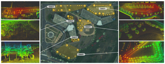
Figure 1.
Overview of the Custom Dataset and data acquisition site. The center panel shows the aerial map of the survey area, with six zones (Zone 1 to Zone 6) highlighted and all annotated tree locations marked by yellow circles and unique IDs. Each zone was surveyed using a four-wheel drive mobile robot equipped with LiDAR and IMU sensors. Side panels display representative LiDAR point cloud views from each zone, illustrating the diversity in tree arrangements and environmental conditions.
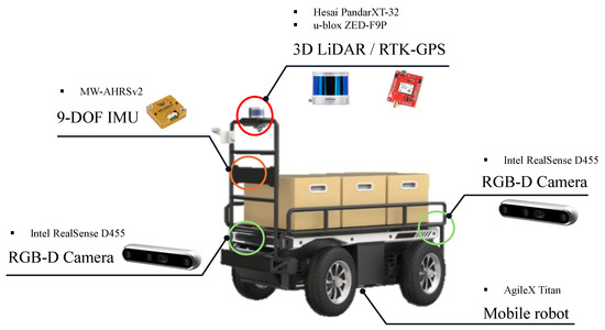
Figure 2.
Configuration of the mobile robot platform for data collection. Only the Hesai PandarXT-32 3D LiDAR and MW-AHRSv2 9-DOF IMU were used as primary sensors for dataset acquisition; the other mounted sensors served as auxiliary components and were not used in this work.
In total, the dataset comprises 64 individual tree samples distributed across six zones. Mean DBH by zone ranges from 11.6 cm to 35.0 cm, and mean perimeter from 37.9 cm to 109.9 cm. Full statistics including standard deviation, minimum, and maximum values are given in Table 1. Figure 3 summarizes the per-zone counts and DBH distributions. For each tree, ground-truth perimeter and DBH were manually measured at a height of 1.37 m above ground by the same annotator. Each measurement was repeated twice, and the average value was recorded to ensure consistency and accuracy (Figure 4). The tree IDs and positions are mapped based on coordinate information and overlaid on aerial imagery, along with example LiDAR point cloud scenes collected from each zone (Figure 1).

Table 1.
Zone-wise statistics of tree DBH and perimeter (both in centimeters) in the constructed dataset.
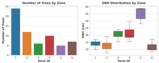
Figure 3.
Distribution of the number of trees (left) and DBH values (right) for each zone in the constructed dataset.
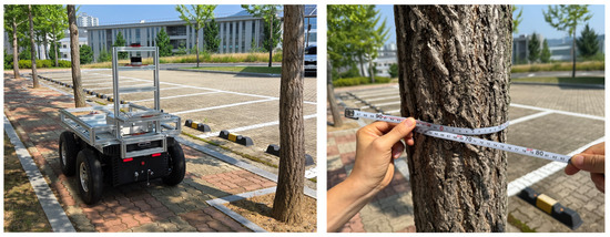
Figure 4.
Data collection procedures. (Left) Manual teleoperation of the mobile robot for LiDAR/IMU mapping. (Right) Manual measurement of stem perimeter at breast height of 1.37 m using a tape measure.
The dataset includes diverse tree species and environments commonly found in urban settings. It includes trees with a wide range of diameters and multiple species, such as Ginkgo biloba (ginkgo), Zelkova serrata (zelkova), Chionanthus retusus (Chinese fringe tree), Quercus spp. (oak), and Pinus spp. (pine). Data were collected in a variety of environments, ranging from open areas (e.g., parking lots and gardens) to occluded zones near buildings or along property boundaries. The presence of parked vehicles, fences, and other urban infrastructure includes common urban features that affect mapping and DBH estimation.
For evaluation, each sample is paired with ground-truth DBH and perimeter measurements, spatial position, and a segmented LiDAR point cloud. The dataset is organized with per-tree annotations and raw sensor recordings to support reproducible analysis. Summary statistics by zone are shown in Figure 3 and Table 1.
2.2. Robust DBH Estimation with Minimal Shape Priors
In conventional fieldwork, DBH is measured by wrapping a tape around the tree trunk, recording its perimeter, and dividing that length by [9,24]. Our pipeline instead directly estimates the stem cross-section’s perimeter from the LiDAR point cloud and converts it to DBH. This approach avoids the strong geometric assumptions imposed by circle or ellipse fitting, which can introduce bias when the cross-section is irregular or the scan data are incomplete. Accordingly, our pipeline is designed with three core objectives: robustness to partial or sparse data, insensitivity to deviations from circularity, and minimal reliance on predefined shape priors (Figure 5, Algorithm 1).
| Algorithm 1: Sector-Based Perimeter Reconstruction Pipeline for DBH Estimation |
 |
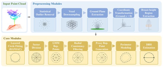
Figure 5.
Overview of the DBH estimation pipeline. The method extracts a 2D cross-section at breast height from a 3D point cloud and estimates the diameter by modeling the perimeter with filtered and symmetrically extended representative points.
Starting from the pre-processed breast height slice (Section 2.2.1), the center of the stem cross-section is refined using a RANSAC-based layered circle fitting algorithm [12,29] (Section 2.2.2). The horizontal plane is subsequently partitioned into m equal-angle angular sectors (Section 2.2.3). Within each sector, a Gaussian Mixture Model (GMM) [32] is employed to identify a single representative point (Section 2.2.4). A radial consistency filter is applied to remove anomalous sectors (Section 2.2.5). When a sector lacks a valid representative point, it is completed by mirroring the point from the diametrically opposite sector, leveraging the approximate radial symmetry of tree stems (Section 2.2.6).
The resulting set of m representative points is used to estimate the stem’s cross-sectional perimeter via two complementary models: the convex hull [33] and the closed B-spline [34], as detailed in Section 2.2.7. Let L denote the estimated perimeter from either model; the diameter is then computed as
The proposed method first refines the stem center using a multi-layer RANSAC [36] circle fit. It then extracts representative points sector by sector and reconstructs any missing sectors through symmetry. Finally, it models the perimeter to compute DBH. This sequence produces accurate and robust diameter estimates, even when the LiDAR data are noisy or incomplete.
2.2.1. Preprocessing Pipeline for DBH Region Extraction
The preprocessing pipeline begins by cropping each tree’s full-scan point cloud to a cylindrical region centered on its approximate trunk axis, defined by a fixed horizontal radius and vertical bounds. The resulting subset is then denoised using the Statistical outlier removal method implemented in Open3D [37]: For each point, the mean distance to its k nearest neighbors is computed, and points whose mean distance exceeds the global mean plus a user-defined multiple of the standard deviation are discarded. Voxel downsampling is applied to the denoised point cloud using a cubic leaf size v. All points within each voxel are replaced by their centroid to reduce data redundancy and improve downstream processing efficiency. Ground plane estimation is performed on the downsampled cloud using RANSAC [36]. The entire point cloud is then translated vertically so that the fitted ground plane lies at , establishing a consistent ground reference across all trees. Finally, we retain points within a narrow vertical band above the ground (e.g., ) and define the DBH cross-section as the horizontal projection of these points (Figure 6). This vertical-band projection increases cross-sectional point density and improves robustness to sparse sampling at exactly , so subsequent representative points are derived from the projection rather than constrained to lie on the exact plane. Within the window around breast height, stems are well approximated by a near linear taper, with typical species-level stem taper rates of about 0.011–0.017 m/m [38], indicating that the cross-sectional radius changes only gradually with height. Projecting this narrow band to the horizontal plane therefore yields a stable estimate of the breast-height cross-section perimeter. This approach mitigates sparsity and occlusion at exactly without relying on a single-height slice.
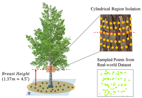
Figure 6.
Output of the preprocessing stage: cylindrical region extraction at breast height (1.37 m) for stem cross-section analysis. The zoomed views show schematic sampling of the cylindrical surface (top-right) and actual LiDAR points extracted from a real dataset (bottom-right).
2.2.2. Layered Circular Fitting for Cross-Sectional Center Refinement
Starting from the breast height band defined in Section 2.2.1, we generate a small stack of thin horizontal layers to refine the cross-sectional center. Let the dataset-specific breast height be . Layers are centered at
which yields five layers at 5 cm spacing (Figure 7). For each , we extract points within a thin slab
and within a horizontal radius from the initial center estimate.
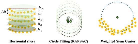
Figure 7.
Multi-layer RANSAC-based estimation of the stem center. Horizontal slices near breast height are processed with RANSAC to estimate provisional centers, which are fused via inlier-weighted averaging. Excessive deviation from the initial center triggers fallback to the original estimate.
On each horizontal slice, RANSAC is applied to fit a circle in the 2D plane. We perform at most iterations with a residual threshold . Fits are retained only if they have at least inliers and a plausible radius range . Each accepted fit yields a center and an inlier count .
The final center estimate is computed as the inlier-weighted average of the valid circle centers:
which assigns greater influence to layers exhibiting stronger geometric support. To guard against spurious estimates, the displacement between the refined center and the initial estimate is compared to the search radius . If this displacement exceeds , the initial center is retained.
This RANSAC-based refinement yields a robust and geometrically consistent estimate of the stem’s cross-sectional center, which serves as a reliable reference point for subsequent perimeter modeling and DBH estimation.
2.2.3. Angular Segmentation of Stem Cross-Section
To achieve uniform sampling of the stem’s cross-sectional boundary and to extract representative points, the horizontal slice at breast height is partitioned into m angular sectors centered at the refined stem center (Figure 8). To suppress spurious noise near the center, we restrict attention to points within a radial band:
where and define the minimum and maximum radial limits of the region of interest. For each , its azimuth angle is computed as
and the corresponding sector index is assigned via
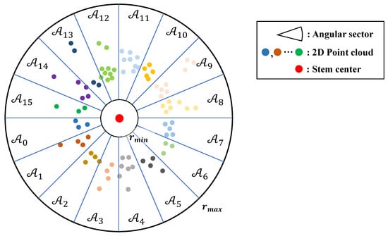
Figure 8.
Angular segmentation of the breast height cross-section. The point set P is divided into m equal-angular sectors , from which the subsets are extracted for representative point selection within each sector.
The kth sector is then defined as
where each sector spans an angular width of , ensuring a uniform and non-overlapping partition of the circular cross-section. The set of points assigned to the kth sector is denoted by . This segmentation strategy guarantees angular uniformity and also provides a natural framework for handling missing or sparse regions: if a sector contains no valid points, it can later be supplemented via symmetry (Section 2.2.6).
2.2.4. Sector-Level Representative Point Estimation via Gaussian Mixture Modeling
After partitioning the cross-section into m angular sectors (Section 2.2.3), each sector contains a set of 2D points projected onto the horizontal plane. These sector-wise point sets originate from aggregated MLS scans and can be affected by measurement noise from scan-time motion distortion and residual registration errors [39,40]. Through our experiments, we observed that such noise often appears as sparse points positioned slightly outside the actual stem boundary, even after basic filtering. Such outward-biased samples can distort the reconstructed perimeter if chosen as representatives. To reduce their influence, we combine probabilistic clustering with radial sorting and weighting, giving higher priority to points closer to the primary stem surface cluster. To robustly select a single representative point from each sector in the presence of local irregularities and noise, we model as a mixture of K Gaussian components (Figure 9):
where , , and denote the mixing weight, mean, and covariance matrix of the kth component, respectively. The model is fitted using the Expectation–Maximization (EM) algorithm [32]. For each component, the sample with the highest posterior responsibility is then identified:
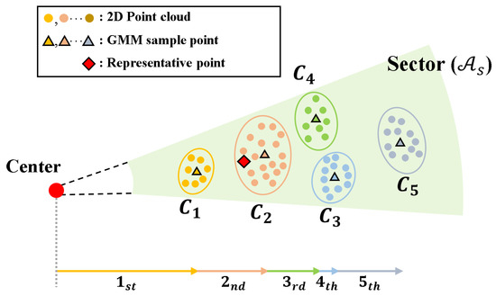
Figure 9.
Representative point estimation within an angular sector using Gaussian Mixture Modeling (GMM). Points in sector are clustered into K Gaussian components, and for each component, the sample with the highest posterior responsibility is selected. These samples are then ranked by their distance to the stem center, assigning higher weights to those closer to the stem center. A weighted average of the ranked samples yields the final representative point for the sector.
Each sample from component k is assigned a cluster-level distance which measures its proximity to the stem center . Because samples nearer the center are presumed more geometrically stable, we assign weights according to their rank in ascending distance: where denotes the rank of in ascending order (i.e., the closest sample receives rank 1). As a result, components whose sample points lie nearer to the stem center are assigned larger weights.
We then combine these rank weights with the GMM mixing weights to define normalized weights:
Finally, the representative point for sector is computed as the weighted average of the component samples:
Within each angular sector, points are clustered with a Gaussian Mixture Model (GMM). For each component, the sample with the highest posterior responsibility is taken as the component representative. Sector representatives are then combined using weights derived from posterior responsibilities and radial ranks relative to the estimated stem center. This approach emphasizes the stem surface at breast height (over-bark), which corresponds to the surface measured in circumference-based DBH. The GMM framework also accounts for the irregular distribution of boundary points within sectors, allowing noise to be down-weighted during representative selection. Similar applications of GMMs to tree point clouds, such as separating trunk or branches from leaves, support its suitability for structure-aware point selection [41]. The resulting set of sector representatives serves as the basis for subsequent perimeter reconstruction.
2.2.5. Radial Consistency-Based Filtering of Representative Points
In practice, radial distance varies smoothly with azimuth at breast height, and adjacent sectors on a single tree stem rarely exhibit abrupt radius changes. The neighbor-gap and global deviation tests encode this geometric expectation, suppressing isolated outward returns that would otherwise inflate the reconstructed perimeter. To detect and correct such anomalies, we apply an after-selection consistency check on sector-wise representative points based on distance from the estimated center, removing outward outliers (Figure 10).
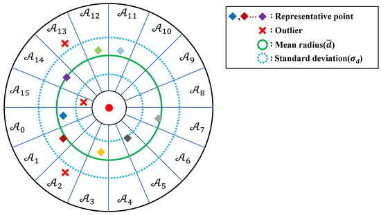
Figure 10.
Radial consistency-based filtering of sector-wise representative points. Each representative point’s distance to the stem center is evaluated, and sectors with anomalous points are detected using two criteria: (1) a local neighbor-gap test that compares distance jumps across adjacent sectors, and (2) a global deviation test that identifies points with large deviations from the overall distribution. Detected outlier sectors (red) are later corrected through symmetry or interpolation.
Let denote the representative point in sector , and let be the estimated stem center. The radial distance from the center is computed as
We compute the following summary statistics over the set : the mean , standard deviation , and median ,
To identify radial inconsistencies, we apply two complementary tests:
- Neighbor-Gap Test: For each sector , define the maximum radial difference relative to its immediate neighbors,with circular indexing (). A sector is flagged as an outlier if , where is a user-defined threshold.
- Global Deviation Test: Compute a standardized deviation score for each sector,and deem an outlier if , where is a user-defined threshold.
The set of detected outlier sectors is defined as
For each outlier sector, the corresponding representative point is later corrected via symmetry or interpolation to restore geometric consistency (Section 2.2.6).
2.2.6. Symmetry-Aware Reconstruction of Missing Representative Points
Some sectors have no valid representative point because all points in that sector were either missing or removed as outliers (Section 2.2.5). To maintain uniform angular coverage and leverage the approximate radial symmetry of tree stems [31], such sectors are populated by mirroring the representative point from the diametrically opposite sector (Figure 11).
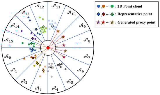
Figure 11.
Proxy generation via radial reflection. Missing or outlier sectors are filled by reflecting a valid representative point from the diametrically opposite sector and adjusting the result to lie within the target sector’s angular bounds.
Let m be the total number of angular sectors and the estimated center of the stem cross-section. Let s be the index of a missing or invalid sector, and define its opposite index as
If the opposite sector contains a valid representative point , we compute a reflected proxy by radial symmetry:
We then verify whether the azimuth of lies within the angular bounds of sector . Let be the angle of point p with respect to , and define the sector’s angular bounds:
If , we instead construct a radial proxy on the sector bisector:
The final augmented representative point is selected as follows:
Under partial occlusion, a missing sector is filled by reflecting the representative from the sector on the opposite side of the stem about the estimated center. If the reflected point falls outside the target sector’s angular bounds, a radial proxy is placed on the sector bisector with the same radius. When both a sector and its opposite are empty, which was rare in our datasets, the sector is omitted and the perimeter is fitted using the remaining representatives. This local procedure preserves angular coverage where possible, maintains geometric consistency, and reduces directional bias. The design relies on the empirically observed smooth variation in radial distance with azimuth at breast height.
2.2.7. Perimeter and DBH Estimation via Convex Hull and B-Spline Models
Given the ordered set of m representative points on the breast height plane, we estimate the stem perimeter using two complementary geometric models (Figure 12).
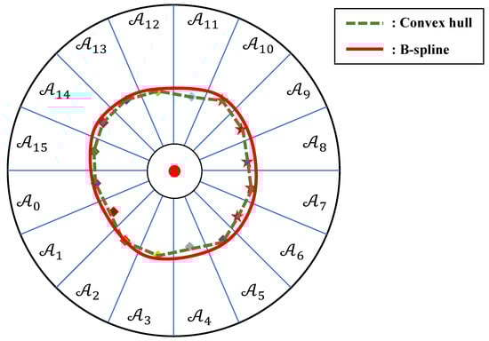
Figure 12.
Stem perimeter estimation using convex hull and B-spline models. The ordered set of representative points is used to construct both a polygonal contour (convex hull) and a smooth closed curve (B-spline), each yielding a distinct estimate of the stem perimeter.
First, we compute the convex hull of , yielding a sequence of vertices arranged in counter-clockwise order, with . The polygonal perimeter is then obtained as
which serves as a fast and gap-tolerant upper bound, since concave intrusions are ignored by definition.
Second, a closed B-spline curve of degree is fitted through the same point set , with parameter . Uniform sampling of this curve at for , with , yields a smoothed estimate of the perimeter:
The convex hull model guards against underestimation caused by missing concave segments, while the B-spline model mitigates the overestimation associated with purely polygonal fits. Given that tree stems are commonly assumed to have circular cross-sections at breast height in forestry practice, the corresponding diameter is computed via the standard relation . Hence,
These two estimates represent the diameters of the best-fitting circles under each perimeter model, and are compared against manual tape measurements for accuracy assessment.
3. Results
3.1. DBH Estimation Accuracy on Benchmark Datasets
The proposed sector-based perimeter reconstruction method was evaluated on three benchmark LiDAR datasets: UCM-0523M and VAT-0723M from the publicly available TreeScope dataset [21], and a Custom Dataset collected and annotated as part of this study. The three benchmarks span a wide range of effective sampling densities and arc completeness, and the fixed configuration achieved consistent accuracy under both sparser (UCM-0523M) and denser (VAT-0723M) conditions (Table 2).
Table 2.
Quantitative comparison of DBH RMSE, relative RMSE, MAE, and DBH statistics between the DBCRE baseline and our method on three datasets: UCM-0523M and VAT-0723M from the publicly available TreeScope dataset [21], and our own Custom Dataset. UCM-0523M uses a 0.3 m bole height, while VAT-0723M and the Custom Dataset use the standard 1.37 m breast height. N indicates the number of tree samples, and bold values indicate the best (lower is better) result within each dataset.
The UCM-0523M dataset is characterized by sparse point density and frequent partial-arc visibility. Only 61.4% of trees exhibit full circular coverage at breast height. In such cases, geometric fitting approaches like DBCRE tend to suffer from large estimation variance due to incomplete contour observations. Our method addresses this issue by interpolating across occluded segments using proxy points, yielding a 0.59 cm reduction in RMSE (from 2.60 to 2.01 cm). Qualitative results (Figure 13) confirm that the reconstructed perimeter remains geometrically plausible even with substantial data loss.
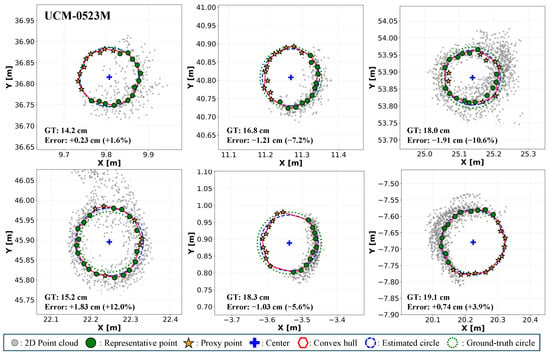
Figure 13.
Qualitative results of the proposed sector-based perimeter reconstruction on six sample trees from the UCM-0523M dataset, illustrating performance under varying scan completeness and noise conditions.
In VAT-0723M, which provides higher point density and spans a wider range of DBH values (20.1–45.0 cm), our pipeline reduces RMSE by 1.20 cm compared to the baseline. This improvement is largely attributed to the radial consistency filtering step, which removes peripheral outliers caused by nearby canopy structures and closely spaced stems prior to perimeter reconstruction (Figure 14).
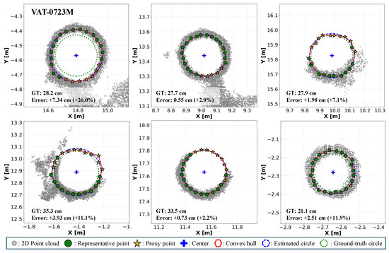
Figure 14.
Qualitative performance of the proposed sector-based perimeter reconstruction on six sample trees from the VAT-0723M dataset, demonstrating accurate diameter recovery under high-density scans and partial-arc occlusion conditions.
The Custom Dataset covers diverse conditions, including multiple tree species, varying spatial layouts, and urban structures. These factors create a rigorous benchmark for DBH estimation. Despite occlusions from objects such as fences and vehicles, our method achieved the lowest RMSE (1.52 cm) and MAE (1.13 cm) among all evaluated approaches. This performance demonstrates consistent accuracy across diverse field conditions. The use of angular sector-based sampling and symmetry-aware reconstruction supports generalization under differences in species, occlusion, and structural layout (Figure 15). The relative RMSE was reduced by 64.5% (from 13.32% to 4.73%), confirming the robustness of the proposed method.
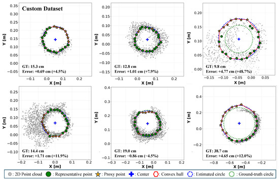
Figure 15.
Qualitative results of the sector-based perimeter reconstruction pipeline on six sample trees from the Custom Dataset, highlighting robustness to varied species, point-density distributions, and partial-arc occlusions.
Most samples in our datasets conform well to the radial symmetry assumption used in proxy point reconstruction. A small number of stems showed degraded performance due to irregular or asymmetric cross-sections. Examples include Figure 13 (first row, third column) and Figure 15 (first row, third column; second row, third column), where mirrored points were misplaced because symmetry was absent, causing the reconstructed contour to deviate from the true boundary. Concave deformations further reduced fitting accuracy in Figure 15 (second row, third column). In rare cases where both a sector and its opposite lacked valid points due to severe occlusion or view geometry (e.g., Figure 13, second row, second column), reconstruction proceeded from the remaining sectors to preserve continuity. These cases were occasional, as illustrated in the examples with overlaid ground-truth (GT) and error values in Figure 13, Figure 14 and Figure 15.
Despite these cases, the full pipeline delivers consistent gains in both accuracy and stability. It combines representative point selection via GMMs, outlier filtering and proxy synthesis (Figure 16). These results are further supported by ablation studies (Section 3.4), which verify the contribution of each core module. Overall, the method outperforms traditional geometric fitting techniques under varied occlusion and environmental conditions (Table 2).
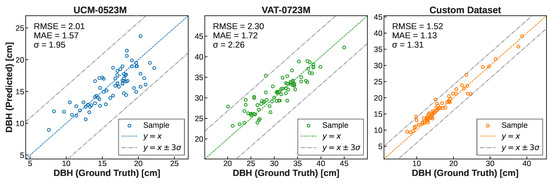
Figure 16.
Predicted vs. ground-truth DBH for three datasets (UCM-0523M, VAT-0723M, Custom Dataset). Dashed lines indicate and .
3.2. Comparison of Perimeter Reconstruction Models
We compared two perimeter reconstruction methods, convex hull and B-spline fitting, using the same set of sector-wise representative and proxy points. The convex hull provides stable performance by enclosing the outermost points without assuming smoothness, making it robust to occlusion, irregular spacing, and sector-level noise.
The B-spline fits a smooth, closed curve through all representative points, enabling it to capture local curvature and interpolate across small gaps. While effective under dense and evenly spaced angular distributions, it may overfit when sector populations are imbalanced or proxy points are irregularly distributed, often leading to diameter overestimation (Figure 17). However, in partial scans where the available points form a coherent arc with consistent radial spacing, the B-spline can produce tighter and more accurate perimeter reconstructions than the convex hull. This advantage is reflected in UCM-0523M, where the B-spline achieves lower RMSE despite increased occlusion (Table 3). Taken together, convex hulls are reliable under field noise and sparsity, while B-splines are preferable in well-sampled conditions.
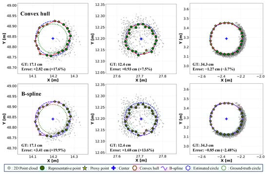
Figure 17.
Qualitative comparison of Convex hull (top row) and B-spline (bottom row) perimeter reconstructions on three sample trees. In Samples 1 and 2 (left and center), the B-spline (magenta) closely follows sector-level fluctuations, occasionally resulting in overestimated diameters. In Sample 3 (right), the B-spline smoothly interpolates across sparse or occluded segments, producing a tighter fit and more accurate diameter estimate.
Table 3.
Quantitative comparison of DBH estimation performance using two different perimeter modeling methods: convex hull and B-spline. All experiments use the same DBH estimation pipeline proposed in this work, with the only difference being the perimeter reconstruction technique. N indicates the number of tree samples, and bold values indicate the best (lower is better) result within each dataset.
3.3. Analysis of Key Parameter Configurations
To assess the impact of key configuration choices on DBH estimation performance, we analyzed three parameters: the number of angular sectors (m), the number of GMM components per sector (K), and the spline degree () for B-spline perimeter reconstruction (Table 4). Unless otherwise noted, parameter sweeps for m and K were conducted with the convex hull perimeter model, fixing the other settings at m = 24 and K = 5. When evaluating the B-spline perimeter model, we fixed m = 24 and K = 5 and varied to assess its effect on perimeter accuracy. This clarifies that is not applicable to convex hull experiments.
Table 4.
Impact of key algorithmic parameters on DBH estimation accuracy across three datasets. “Sectors” refers to the number of angular partitions (m), “GMM comps.” denotes the number of Gaussian components per sector (K), and “B-spline degree” is the degree of the B-spline () used for perimeter reconstruction. Bold values indicate the best (lower is better) result within each dataset.
Our analysis shows that the proposed method performs robustly within a reasonable range of these parameters. When m was reduced below 24, sector sampling became too sparse, degrading boundary coverage. Increasing m above 24 increased susceptibility to local noise in sparsely populated regions. Similarly, setting often failed to capture meaningful point distributions under heterogeneous noise, while risked overfitting to small or spurious clusters. For the B-spline model, no single spline degree is universally optimal. Dataset-wise minima occur at on UCM-0523M, on VAT-0723M, and on the Custom Dataset (Table 4). Higher degrees can introduce oscillations under uneven angular sampling, while lower degrees may over-smooth curvature in well-sampled arcs.
These results demonstrate that the default parameter settings provide an effective balance between generalization and accuracy across diverse forest environments. In datasets characterized by nonstandard point densities or elevated noise levels and irregular occlusion, targeted tuning of m and K yields additional performance gains.
3.4. Ablation Study: Impact of Individual Core Pipeline Components
To assess the contribution of each core module, we conducted ablation experiments by selectively disabling (i) GMM-based representative point selection, (ii) radial consistency filtering, and (iii) symmetry-aware proxy point reconstruction across three datasets (Table 5). When all modules were disabled, the average RMSE increased substantially to 4.36 cm, with severe under or overestimation observed across datasets: 2.72 cm on UCM-0523M, 8.38 cm on VAT-0723M, and 1.99 cm on the Custom Dataset.
Table 5.
Ablation study of pipeline components on three test sets. UCM-0523M and VAT-0723M are the orchard and forest subsets of TreeScope [21], and the “Custom Dataset” denotes our own field scans. ✓ indicates the module is enabled, – indicates it is disabled, and bold values indicate the best (lower is better) result within each dataset.
Disabling proxy point reconstruction increased RMSE to 2.36 cm for UCM-0523M, demonstrating the importance of gap compensation in partial-arc scans. On VAT-0723M, radial consistency filtering alone reduced RMSE by 6.02 cm (from 8.38 cm to 2.36 cm), effectively suppressing noise introduced by structural clutter and overlapping stems. In the Custom Dataset, enabling only GMM-based point selection improved the consistency of representative point extraction, leading to a reduction in MAE from 1.56 cm to 1.17 cm.
When all three components were active, they worked synergistically to achieve RMSEs of 2.01 cm (UCM-0523M), 2.30 cm (VAT-0723M), and 1.52 cm (Custom Dataset), demonstrating the pipeline’s robustness across diverse occlusion levels and scan densities. These results confirm that each module contributes uniquely and significantly to the accuracy and reliability of the overall DBH estimation framework.
4. Discussion
The proposed sector-based DBH estimation pipeline demonstrates improved accuracy compared to the conventional DBCRE [21] method. Across the three evaluated benchmarks (UCM-0523M, VAT-0723M, and the Custom Dataset), the estimated diameters closely match the ground-truth DBH values. The pipeline divides each stem cross-section into 24 angular sectors ( each). Within each sector, points are clustered using a K-component Gaussian Mixture Model (GMM), and the point with the highest posterior responsibility is selected as the representative. These representative points are then used to reconstruct the perimeter via either a convex hull or a B-spline model.
The GMM enables robust identification of boundary points by modeling the radial distribution of points and suppressing peripheral outliers common in cluttered scans. When a sector lacks valid observations due to occlusion or denoising, a symmetry-aware proxy is generated by reflecting the representative point from the opposite sector. If the reflected point falls outside the angular bounds, an adjusted proxy is placed along the sector bisector to maintain geometric consistency (Table 5).
The choice of perimeter model depends on scan completeness and point density. In VAT-0723M, where sampling is dense but some arcs are missing, the convex hull performs better by tightly enclosing outer points and avoiding overestimation. In contrast, UCM-0523M exhibits more severe occlusions; in such cases, the B-spline provides smoother interpolation across gaps and improves accuracy (Table 3).
Ablation studies confirm the importance of each module. When all three components, namely GMM-based point selection, radial filtering, and proxy synthesis, are enabled, the pipeline achieves the lowest RMSE across datasets. Disabling any module degrades performance. For example, in UCM-0523M, replacing GMM with per-sector median yields similar results due to symmetric noise, while in VAT-0723M, excluding proxy synthesis has limited impact due to dense and complete arcs (Table 5).
A limitation of the proposed pipeline lies in the mirrored-point substitution, which assumes bilateral symmetry in the stem cross-section when replacing missing representative points. While effective for the majority of stems in the evaluated datasets, this assumption may not hold in natural forests where irregular or asymmetric shapes can arise from abnormal growth, scar, or interference from surrounding vegetation. As observed in Figure 13 (first row-third column) and Figure 15 (first row-third column, second row-third column), such violations can cause misplaced proxy points and a shifted reconstructed contour, ultimately reducing DBH estimation accuracy.
Future work will focus on adaptively determining the number of angular sectors based on local point cloud properties such as density and coverage. In addition, we will adjust the number of GMM components according to occlusion levels and other relevant point cloud characteristics. Replacing fixed parameters with data-driven configurations may improve robustness under varying forest structures and scan conditions. This adaptivity is expected to enhance point selection and perimeter reconstruction, especially in regions with uneven data quality.
5. Conclusions
We introduced a perimeter-based pipeline for estimating tree diameter at breast height (DBH) from LiDAR point clouds, targeting key limitations of conventional geometric fitting methods. When stems maintain radial symmetry, conventional circle or ellipse fitting is often sensitive to partial arc visibility, uneven point density, and peripheral outliers, which can distort the estimated center and radius. Our approach addresses these issues by applying angular sector-wise representative point extraction via Gaussian Mixture Models (GMMs), radial consistency filtering, and symmetry-aware proxy generation to compensate for occluded or sparsely sampled sectors. This design improves the stability and accuracy of perimeter reconstruction under both sparse and dense scan conditions.
Experiments on three benchmark datasets, including two TreeScope subsets and a custom field-collected dataset, demonstrated consistent improvements over the baseline DBCRE method, with RMSEs below 2.5 cm. The method maintained robustness across varied occlusion levels, point densities, and urban and natural settings. Ablation studies confirmed that each pipeline component contributed uniquely to performance gains, and comparisons between convex hull and B-spline perimeter models highlighted complementary strengths depending on scan completeness.
Failure cases were observed for stems with irregular or asymmetric cross-sections, where the symmetry-based proxy generation could not fully reconstruct the true perimeter. These cases were identified and discussed in the Results Section, along with qualitative examples. Future work will focus on incorporating shape-adaptive reconstruction strategies to handle non-symmetric geometries and on developing data-driven adaptation of sector partitioning and proxy weighting for more diverse forest and urban conditions.
Author Contributions
Conceptualization, W.K. and H.-S.S.; software, W.K. and S.-Y.A.; writing original draft preparation, W.K. and H.-S.S.; writing review and editing, H.-S.S. and S.-Y.A.; supervision, S.-Y.A. All authors have read and agreed to the published version of the manuscript.
Funding
This work was supported by Electronics and Telecommunications Research Institute (ETRI) grant funded by the Korean government [25ZD1150, Development of ICT Convergence Technology for Daegu-Gyeongbuk Regional Industry].
Data Availability Statement
The custom dataset generated during this research is part of an ongoing project and is not publicly available due to institutional restrictions and to protect the integrity of the continuing work. Access to the dataset may be granted upon reasonable request to the corresponding author, subject to approval by the project coordinators and relevant confidentiality agreements.
Conflicts of Interest
The authors declare no conflicts of interest.
References
- Shao, T.; Qu, Y.; Du, J. A low-cost integrated sensor for measuring tree diameter at breast height (DBH). Comput. Electron. Agric. 2022, 199, 107140. [Google Scholar] [CrossRef]
- Lappi, J. A multivariate, nonparametric stem-curve prediction method. Can. J. For. Res. 2006, 36, 1017–1027. [Google Scholar] [CrossRef]
- Liang, X.; Kankare, V.; Yu, X.; Hyyppä, J.; Holopainen, M. Automated stem curve measurement using terrestrial laser scanning. IEEE Trans. Geosci. Remote Sens. 2013, 52, 1739–1748. [Google Scholar] [CrossRef]
- Kalwar, O.P.; Hussin, Y.A.; Weir, M.J.; De Bie, C.; Karna, Y. Deriving forest plot inventory parameters using terrestrial laser scanning in the tropical rainforest of Malaysia. Int. J. Remote Sens. 2021, 42, 884–901. [Google Scholar] [CrossRef]
- Zhou, R.; Wu, D.; Zhou, R.; Fang, L.; Zheng, X.; Lou, X. Estimation of DBH at forest stand level based on multi-parameters and generalized regression neural network. Forests 2019, 10, 778. [Google Scholar] [CrossRef]
- Austin, D.U.; Yirdaw, E. Models for Predicting Tree Diameter at Breast Height from Over and Under Bark Diameter of Stump in Eucalyptus camaldulensis Plantations. Preprints 2025. [Google Scholar] [CrossRef]
- Hui, Z.; Lin, L.; Jin, S.; Xia, Y.; Ziggah, Y.Y. A reliable dbh estimation method using terrestrial lidar points through polar coordinate transformation and progressive outlier removal. Forests 2024, 15, 1031. [Google Scholar] [CrossRef]
- Ravaglia, J.; Fournier, R.A.; Bac, A.; Véga, C.; Côté, J.F.; Piboule, A.; Rémillard, U. Comparison of three algorithms to estimate tree stem diameter from terrestrial laser scanner data. Forests 2019, 10, 599. [Google Scholar] [CrossRef]
- Sheng, Y.; Zhao, Q.; Wang, X.; Liu, Y.; Yin, X. Tree Diameter at Breast Height Extraction Based on Mobile Laser Scanning Point Cloud. Forests 2024, 15, 590. [Google Scholar] [CrossRef]
- Eliopoulos, N.J.; Shen, Y.; Nguyen, M.L.; Arora, V.; Zhang, Y.; Shao, G.; Woeste, K.; Lu, Y.H. Rapid tree diameter computation with terrestrial stereoscopic photogrammetry. J. For. 2020, 118, 355–361. [Google Scholar] [CrossRef]
- Fu, K.; Yue, S.; Yin, B. DBH Extraction of Standing Trees Based on a Binocular Vision Method. In Proceedings of the 2023 IEEE International Instrumentation and Measurement Technology Conference (I2MTC), Kuala Lumpur, Malaysia, 22–25 May 2023; IEEE: Piscataway, NJ, USA, 2023; pp. 1–6. [Google Scholar]
- Gao, Q.; Kan, J. Automatic forest DBH measurement based on structure from motion photogrammetry. Remote Sens. 2022, 14, 2064. [Google Scholar] [CrossRef]
- Wu, Y.; Gan, X.; Zhou, Y.; Yuan, X. Estimation of Diameter at Breast Height in tropical forests based on Terrestrial Laser Scanning and shape diameter function. Sustainability 2024, 16, 2275. [Google Scholar] [CrossRef]
- Hu, C.; Pan, S.; Zhang, H.; Li, P. Trunk model establishment and parameter estimation for a single tree using multistation terrestrial laser scanning. IEEE Access 2020, 8, 102263–102277. [Google Scholar] [CrossRef]
- Liu, L.; Zhang, A.; Xiao, S.; Hu, S.; He, N.; Pang, H.; Zhang, X.; Yang, S. Single tree segmentation and diameter at breast height estimation with mobile LiDAR. IEEE Access 2021, 9, 24314–24325. [Google Scholar] [CrossRef]
- Liu, G.; Wang, J.; Dong, P.; Chen, Y.; Liu, Z. Estimating individual tree height and diameter at breast height (DBH) from terrestrial laser scanning (TLS) data at plot level. Forests 2018, 9, 398. [Google Scholar] [CrossRef]
- Wang, A.; Wang, J.; Li, H.; Hu, J.; Zhou, H.; Zhang, X.; Liu, X.; Wang, W.; Zhang, W.; Wu, S.; et al. Tree parameter extraction method based on new remote sensing technology and terrestrial laser scanning technology. Big Data Res. 2024, 36, 100460. [Google Scholar] [CrossRef]
- Guenther, M.; Heenkenda, M.K.; Morris, D.; Leblon, B. Tree Diameter at Breast Height (DBH) Estimation Using an iPad Pro LiDAR Scanner: A Case Study in Boreal Forests, Ontario, Canada. Forests 2024, 15, 214. [Google Scholar] [CrossRef]
- Wang, P.; Gan, X.; Zhang, Q.; Bu, G.; Li, L.; Xu, X.; Li, Y.; Liu, Z.; Xiao, X. Analysis of parameters for the accurate and fast estimation of tree diameter at breast height based on simulated point cloud. Remote Sens. 2019, 11, 2707. [Google Scholar] [CrossRef]
- USDA Forest Service. Forest Inventory and Analysis National Core Field Guide Volume I: Field Data Collection Procedures for Phase 2 Plots, Version 7.0; USDA Forest Service: Arlington, VA, USA, 2011; p. 114.
- Cheng, D.; Cladera, F.; Prabhu, A.; Liu, X.; Zhu, A.; Green, P.C.; Ehsani, R.; Chaudhari, P.; Kumar, V. Treescope: An agricultural robotics dataset for lidar-based mapping of trees in forests and orchards. In Proceedings of the 2024 IEEE International Conference on Robotics and Automation (ICRA), Yokohama, Japan, 13–17 May 2024; IEEE: Piscataway, NJ, USA, 2024; pp. 14860–14866. [Google Scholar]
- Henning, J.G.; Radtke, P.J. Detailed stem measurements of standing trees from ground-based scanning lidar. For. Sci. 2006, 52, 67–80. [Google Scholar] [CrossRef]
- Prabhu, A.; Liu, X.; Spasojevic, I.; Wu, Y.; Shao, Y.; Ong, D.; Lei, J.; Green, P.C.; Chaudhari, P.; Kumar, V. UAVs for forestry: Metric-semantic mapping and diameter estimation with autonomous aerial robots. Mech. Syst. Signal Process. 2024, 208, 111050. [Google Scholar] [CrossRef]
- Putra, B.T.W.; Ramadhani, N.J.; Soedibyo, D.W.; Marhaenanto, B.; Indarto, I.; Yualianto, Y. The use of computer vision to estimate tree diameter and circumference in homogeneous and production forests using a non-contact method. For. Sci. Technol. 2021, 17, 32–38. [Google Scholar] [CrossRef]
- Tinkham, W.T.; Swayze, N.C.; Hoffman, C.M.; Lad, L.E.; Battaglia, M.A. Modeling the missing DBHs: Influence of model form on UAV DBH characterization. Forests 2022, 13, 2077. [Google Scholar] [CrossRef]
- Sumnall, M.J.; Raigosa-Garcia, I.; Carter, D.R.; Albaugh, T.J.; Campoe, O.C.; Rubilar, R.A.; Alexander, B.; Cohrs, C.W.; Cook, R.L. Assessing Methods to Measure Stem Diameter at Breast Height with High Pulse Density Helicopter Laser Scanning. Remote Sens. 2025, 17, 229. [Google Scholar] [CrossRef]
- Fu, L.; Duan, G.; Ye, Q.; Meng, X.; Luo, P.; Sharma, R.P.; Sun, H.; Wang, G.; Liu, Q. Prediction of individual tree diameter using a nonlinear mixed-effects modeling approach and airborne LiDAR data. Remote Sens. 2020, 12, 1066. [Google Scholar] [CrossRef]
- Paris, C.; Bruzzone, L. A growth-model-driven technique for tree stem diameter estimation by using airborne LiDAR data. IEEE Trans. Geosci. Remote Sens. 2018, 57, 76–92. [Google Scholar] [CrossRef]
- Proudman, A.; Ramezani, M.; Fallon, M. Online estimation of diameter at breast height (DBH) of forest trees using a handheld LiDAR. In Proceedings of the 2021 European Conference on Mobile Robots (ECMR), Bonn, Germany, 31 August–3 September 2021; IEEE: Piscataway, NJ, USA, 2021; pp. 1–7. [Google Scholar]
- Liang, X.; Litkey, P.; Hyyppa, J.; Kaartinen, H.; Vastaranta, M.; Holopainen, M. Automatic stem mapping using single-scan terrestrial laser scanning. IEEE Trans. Geosci. Remote Sens. 2011, 50, 661–670. [Google Scholar] [CrossRef]
- Włoch, W.; Iqbal, M.; Jura-Morawiec, J. Calculating the growth of vascular cambium in woody plants as the cylindrical surface. Bot. Rev. 2023, 89, 237–249. [Google Scholar] [CrossRef]
- Xu, L.; Jordan, M.I. On convergence properties of the EM algorithm for Gaussian mixtures. Neural Comput. 1996, 8, 129–151. [Google Scholar] [CrossRef]
- Barber, C.B.; Dobkin, D.P.; Huhdanpaa, H. The quickhull algorithm for convex hulls. ACM Trans. Math. Softw. 1996, 22, 469–483. [Google Scholar] [CrossRef]
- Eilers, P.H.; Marx, B.D. Flexible smoothing with B-splines and penalties. Stat. Sci. 1996, 11, 89–121. [Google Scholar] [CrossRef]
- Chen, K.; Nemiroff, R.; Lopez, B.T. Direct lidar-inertial odometry: Lightweight lio with continuous-time motion correction. In Proceedings of the 2023 IEEE international conference on robotics and automation (ICRA), London, UK, 29 May–2 June 2023; IEEE: Piscataway, NJ, USA, 2023; pp. 3983–3989. [Google Scholar]
- Se, S.; Brady, M. Ground plane estimation, error analysis and applications. Robot. Auton. Syst. 2002, 39, 59–71. [Google Scholar] [CrossRef]
- Zhou, Q.Y.; Park, J.; Koltun, V. Open3D: A modern library for 3D data processing. arXiv 2018, arXiv:1801.09847. [Google Scholar] [CrossRef]
- Larsen, D.R. Simple taper: Taper equations for the field forester. In Proceedings of the 20th Central Hardwood Forest Conference, Columbia, MO, USA, 28 March 28–1 April 2016; General Technical Report NRS-P-167. US Department of Agriculture, Forest Service, Northern Research Station: Newtown Square, PA, USA, 2017; pp. 265–278. [Google Scholar]
- Zhang, J.; Singh, S. LOAM: Lidar odometry and mapping in real-time. Robot. Sci. Syst. 2014, 2, 1–9. [Google Scholar]
- Shan, T.; Englot, B.; Meyers, D.; Wang, W.; Ratti, C.; Rus, D. Lio-sam: Tightly-coupled lidar inertial odometry via smoothing and mapping. In Proceedings of the 2020 IEEE/RSJ international conference on intelligent robots and systems (IROS), Las Vegas, NV, USA, 24 October 2020–24 January 2021; IEEE: Piscataway, NJ, USA, 2020; pp. 5135–5142. [Google Scholar]
- Belton, D.; Moncrieff, S.; Chapman, J. Processing tree point clouds using Gaussian Mixture Models. ISPRS Ann. Photogramm. Remote Sens. Spat. Inf. Sci. 2013, 2, 43–48. [Google Scholar] [CrossRef]


Disclaimer/Publisher’s Note: The statements, opinions and data contained in all publications are solely those of the individual author(s) and contributor(s) and not of MDPI and/or the editor(s). MDPI and/or the editor(s) disclaim responsibility for any injury to people or property resulting from any ideas, methods, instructions or products referred to in the content. |
© 2025 by the authors. Licensee MDPI, Basel, Switzerland. This article is an open access article distributed under the terms and conditions of the Creative Commons Attribution (CC BY) license (https://creativecommons.org/licenses/by/4.0/).