Abstract
Under the dual pressures of climate change and anthropogenic activities, the sustainability of the fragile ecosystem on the Qingzang Plateau has garnered considerable attention. This study, taking the Yarlung Tsangpo River, Lhasa River, and Nianchu River Basin (YNL) of Xizang as a case study, systematically assesses the spatiotemporal evolution of its ecosystem services from 2000 to 2020. It reveals a critical dynamic: while regional ecosystem services have shown an overall improving trend over the past two decades, driven jointly by a warmer and wetter climate and ecological engineering projects, the adverse impacts of human activities have intensified significantly, posing an emerging and growing threat to regional ecological security. Based on the InVEST model, this research quantifies four key services and constructs a Comprehensive Ecosystem Service (CES) index to evaluate the overall ecosystem function. Subsequently, an integrated Principal Component Analysis and Partial Least Squares Structural Equation Modeling (PCA-PLS-SEM) analytical framework is employed to decouple the complex pathways driving CES successfully. The results confirm that climate and topography are the fundamental natural drivers determining the spatial pattern of ecosystem services, which is characterized as being high in the east and low in the west. The core contribution of this study lies in its quantitative identification of the coexisting reality of “ecological improvement” and “development pressure” in the region. It emphasizes that future management strategies must urgently shift from a static conservation approach to an integrated paradigm capable of proactively addressing human–land contradictions. This provides a critical scientific basis for safeguarding China’s national ecological security barrier.
1. Introduction
Ecosystem services (ESs), which provide a fundamental link between human well-being and natural ecosystems, serve as the cornerstone for regional and global sustainable development [1]. However, the combined effects of increased human activity and global climate change are changing ecosystem structure and function at a never-before-seen rate, creating significant and increasing challenges to ecosystems’ ability to provide services [2,3]. On the one hand, major engineering projects, such as large-scale water conservancy hubs, trans-regional transportation networks, and urban agglomeration expansion, represent the most direct and profound human activities altering landscape patterns and natural processes, thereby exerting complex and far-reaching impacts on ecosystem services [4,5]. By changing land use patterns, interfering with hydrological connectivity, and affecting biodiversity, these projects may have a cascade of ecological effects in addition to accomplishing particular socioeconomic objectives. This would reshape the trade-offs and synergies among regional ecosystem services. On the other hand, extreme climate events, including droughts, floods, and heatwaves, are increasing in frequency and intensity globally, directly impacting the stability and resilience of ecosystems and potentially leading to the sharp degradation or even systemic collapse of key services such as water conservation and carbon storage [6]. Because of unsustainable land use practices, around 60% of the world’s ESs have been degraded or have been in danger of collapsing during the previous 50 years [7,8], According to projections, the global demand for food, energy, and water could grow by 40%, 50%, and 35%, respectively, by 2030 [9]. In order to address regional ecological challenges, maintain ecosystem balance, and improve human well-being, it is now critically important to scientifically understand the spatiotemporal evolution of ESs and uncover their driving mechanisms in the complex context of intertwined disturbances from climate change and major engineering projects.
As multiple ecosystem services (ESs) often coexist within the same geographical area [10], an integrated assessment of multiple ESs has become a key approach for understanding social–ecological system interactions and achieving sustainable management [11]. In recent years, model-based quantitative and fine-grained assessment methods have gained mainstream acceptance. Among them, the InVEST model, with its advantage of integrating remote sensing technology, enables the spatiotemporal quantification and visualization of ES functions. Numerous macro-scale pattern studies of modules, including as carbon sequestration, habitat quality, water production, and soil conservation, have made substantial use of it [12]. Current studies have predominantly focused on individual ecosystem services [13,14] or on a limited combination of services [15,16]. However, a considerable body of research emphasizes integrated assessments that combine key ecosystem functions such as carbon sequestration, soil conservation, and water yield. Focusing on a narrow set of services may lead to an incomplete understanding of ecosystem functionality. Therefore, there is an urgent need to develop a Comprehensive Ecosystem Service (CES) assessment framework that quantitatively integrates diverse ecosystem services to better inform decision-making for integrated ecological management.
Numerous anthropogenic and natural variables work together to create changes in ESa. By affecting biological processes like precipitation and terrain, natural forces establish the baseline pattern of ES supply [17], while this pattern is significantly altered by human activity. Ecosystem evolution is usually a complicated, non-linear process that is caused by the combined influence of many causes [12,18]. Although methods such as correlation analysis and the Geodetector model [19] have been used to quantify driving factors, these traditional statistical methods have limitations in explaining the complex interactions and causal pathways among system elements. They are particularly susceptible to issues of multicollinearity when multiple drivers are highly correlated, which can compromise the reliability of the model results. Therefore, in order to understand the intricate driving factors underlying ES changes, it is imperative to incorporate more rigorous analytical models.
The YNL Basin of Xizang, serving as a key area for ecological resettlement and the core of economic development on the Qingzang Plateau, supports approximately one-third of the autonomous region’s population on just 5.5% of its land area, making its social–ecological system highly sensitive. The region’s ability to grow sustainably has been seriously hampered in recent years by ecological issues brought on by climate change and human activity, such as land desertification, glacier retreat, and grassland degradation. In light of this, this research develops an integrated evaluation and attribution methodology to specifically address the pressing need for ecological conservation in the YNL Basin. First, to address the limitation of current ecological assessments that often focus on single services, this research uses the internationally recognized InVEST model to spatially quantify four key services: water yield, soil conservation, carbon sequestration, and habitat quality. On this basis, considering the combined effects of different services and in the absence of a consensus weighting scheme, a Comprehensive Ecosystem Service (CES) index is constructed using an equal weighting method, providing a more comprehensive view of the region’s overall spatiotemporal ecosystem functions function evolution. Second, to overcome the bottlenecks of traditional statistical methods in analyzing complex driving mechanisms (such as multicollinearity), this study introduces an integrated “PCA-PLS-SEM” model. Prior to employing PLS-SEM to extensively evaluate the direct and indirect paths and strengths of natural variables (such as climate and topography) and human activities on CES change, this technique conducts exploratory analysis using PCA to identify the key driving factors. In order to support decision-making for the creation of scientifically sound ecological protection and sustainable development plans for this vulnerable region, this study will use these techniques to methodically clarify the evolutionary trends and underlying driving mechanisms of ecological services in the region under study between 2000 and 2020.
Accordingly, this study focuses on the “One River and Two Streams” region and proposes an integrated PCA-PLS-SEM analytical framework to identify the key driving factors influencing the Comprehensive Ecosystem Service (CES) index under the combined effects of natural conditions and human activities. The CES index was derived based on the outputs of the InVEST and the Revised Universal Soil Loss Equation (RUSLE) models, which were applied to simulate typical ecosystem services in the region during the period from 2000 to 2020. In addition, spatial autocorrelation analysis was employed to reveal the spatial dependence and clustering patterns of ecosystem services across the study area. The main objectives of this study are as follows: (1) to analyze the spatiotemporal variations in four typical ecosystem services in the study area using the InVEST and RUSLE models; (2) to construct a Comprehensive Ecosystem Services index by equally weighting the four services, and to explore its spatial clustering characteristics through spatial autocorrelation analysis; and (3) to identify the major natural and anthropogenic drivers of CESs by applying PCA-PLS-SEM.
2. Dataset and Methods
2.1. Study Area
The Yarlung Tsangpo River serves as the axis of the YNL Basin of Xizang, which is located in the south-central region of the Xizang Autonomous Region. It connects Sangri County in the Shannan Region to Lhazhi County in the Shigatse Region. The altitude ranges in height from 3306 to 7014 m, with the center and northeastern portions being lower and the north and south being higher (Figure 1). It is about 245.5 km long in all. The average annual temperature ranges from 4.7 to 8.3 °C, with the warmest month’s average temperature being between 10 and 16 °C and the coldest month’s average being between −12 and 0 °C. Precipitation typically ranges between 150 and 540 mm each year. Due to highland ecological resettlement programs, rapid economic expansion, and regional urbanization, the population of the study area has been increasing recently. The region is rich in mineral and tourist resources, and it is renowned as the birthplace of Xizang culture, the center of Xizang’s agricultural production area, and the “Golden Triangle.” It is a significant river valley agricultural zone and a concentrated, overlapping area for farming, animal husbandry, and related auxiliary industries in Xizang, with fertile land making up more than 60% of the entire area.
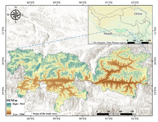
Figure 1.
A map of the geographic location.
2.2. Dataset
The USGS Landsat series products (Landsat-5 TM and Landsat-8 OLI remote sensing images at a resolution of 30 m × 30 m) were used to collect the land use data. Remote sensing images for the study area from May to September for three distinct periods, 2000, 2010, and 2020 (including image data from the preceding and succeeding years for each target year), were downloaded, and images with less than 10% cloud cover were selected. For images in high-cloud areas, high-quality remote sensing images from the same period in the adjacent year (±1 year) were used as substitutes to obtain comprehensive, high-quality imagery for the study area. Following this method, a total of 24 high-quality remote sensing images were acquired. Remote sensing picture maps for 2000, 2010, and 2020 were created by pre-processing the data using ENVI 5.3 software and following a methodology that includes geometric accuracy correction, radiometric calibration, atmospheric correction, image mosaicking and clipping, and image fusion. Through a process of image segmentation, the construction of an interpretation knowledge base, and information extraction with accuracy assessment, the ecosystem distribution maps for the study area were interpreted and generated.
Soil type data were sourced from the National Soil Survey of China. These results were digitized and re-identified on a GIS platform and classified using the traditional “genetic soil classification” system, resulting in a total of eight soil orders for the study area. Geomorphological information was obtained from the People’s Republic of China’s Geomorphological Atlas (1:1,000,000). ASTER GDEM V2 (DEM, 30 m resolution), which is available on the Geospatial Data Cloud platform (https://www.gscloud.cn/), is the digital elevation model used in this study. The model data were imported into ArcGIS 10.7 software and processed through several steps, including mosaicking, projection, clipping, and rasterization to obtain the DEM map and geomorphological data for the study area.
The temperature and precipitation data were provided by the National Earth System Science Data Center (https://www.geodata.cn/). The Gross Domestic Product (GDP) and population density (POP) statistics were provided by the Resource and Environment Science and Data Center, the Chinese Academy of Sciences (https://www.resdc.cn/), and they were generated at a one-kilometer geographic resolution. The datasets used in this study are listed in Table 1. This study first conducted preprocessing of the remote sensing datasets required for the analysis. Subsequently, based on land use and remote sensing data, four representative ecosystem services in the study area were evaluated using the InVEST model and a revised universal soil loss equation (RUSLE). A composite ecosystem service index was then constructed using an equal weight approach. Spatial autocorrelation analysis was employed to investigate the spatial clustering patterns of the ecosystem services. Finally, PCA-PLS-SEM was applied to quantitatively identify the key natural and anthropogenic drivers influencing the spatial pattern of integrated ecosystem services. The workflow of this study is shown in Figure 2. Due to differences in the coordinate systems and original spatial resolutions of the raster datasets, all data were first projected to the WGS_1984_Albers coordinate system using GIS spatial analysis tools. Subsequently, the spatial resolution was 26 to a uniform 1000 m using the nearest neighbor method.

Table 1.
Data sources and descriptions (all accessed on 10 December 2024).
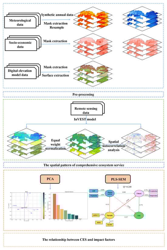
Figure 2.
Technical approach diagram.
2.3. Methods
2.3.1. Ecosystem Service Assessment
- (1)
- Soil Conservation
Soil Conservation (SC) in this study was estimated using the RUSLE method, with the following calculation formula:
In this equation, denotes the amount of soil conservation per unit area (t/hm2·a); R represents the rainfall erosivity factor (MJ·mm·/hm2·a); K is the soil erodibility factor (t·/hm2·a); LS is the topographic factor, which combines slope length and slope steepness; C refers to the vegetation cover and management factor; and P indicates the support practice factor, reflecting the impact of soil and water conservation measures.
The biophysical coefficients required by the model, including the support practice factor (usle_p) and the vegetation cover factor (usle_c), were determined based on previous studies [20,21]. Additionally, “Lucode” represents a unique code assigned to various land use types within the biophysical parameters for soil conservation services (Table 2).
Table 2.
Biophysical parameters of soil conservation services.
- (2)
- Water Yield
To estimate the annual water yield of each grid cell, this study employed the annual water yield module of the InVEST model. The model simulates water yield by subtracting actual evapotranspiration from the annual precipitation. The final water yield consists of multiple hydrological components, including surface runoff, canopy interception, litter water holding capacity, soil moisture content, and groundwater recharge. The calculation process is as follows:
where Yx is the yearly water production (mm) of grid cell x, Px is its yearly precipitation (mm), and AETx is its annual actual evapotranspiration (mm). The estimation of AETx/Px is performed using the Budyko curve equation:
where Z is a seasonality parameter that characterizes the depth and patterns of rainfall, PETx is the annual potential evapotranspiration (mm), Kcx is the plant evapotranspiration coefficient, ETO is the reference evapotranspiration in grid cell x, and AWCX is the plant’s available water content (mm).
In the parameter table, Lucode is the unique code for each ecosystem type, LULC_veg is a vegetation coefficient (0 for non-vegetated and 1 for vegetated), Kc is the ecosystem’s plant evapotranspiration coefficient, which ranges from 0 to 1.5, and root_depth is the root depth. For this study, the biophysical parameter table was compiled by referencing existing research on the Qingzang Plateau [21,22], along with acquired parameters and the Food and Agriculture Organization (FAO) guidelines for crop evapotranspiration coefficients, as detailed in Table 3.
Table 3.
Biophysical quantity parameters of water source conservation services.
The difference between total precipitation and total evapotranspiration is often used to compute regional yearly water conservation. Referencing the calculation method for water conservation in the national guidelines for delineating ecological protection red lines, the formula is as follows:
where, given grid cell x and land cover type j, WRxj is the yearly water conservation. The yearly surface runoff for grid cell x with land cover type j is called Runoffxj. Cj is the surface runoff coefficient for land cover type j.
To isolate the impact of different ecosystem types on water conservation and minimize the influence of precipitation variability, this study used precipitation data from 2000 to calculate water conservation for the years 2000, 2010, and 2020, respectively.
- (3)
- Carbon Storage
This study solely considers the four primary carbon pools—soil organic carbon, dead organic matter, belowground biomass, and aboveground biomass—because there are limited data on forest harvesting. This is how the carbon stock is computed:
where i is a specific ecosystem type and Ci represents the carbon dioxide density of ecosystem type i (t C/hm2). ,, and , respectively, represent the carbon densities of the aboveground, belowground, dead organic matter, and soil carbon pools for ecosystem type i (t C/hm2).
where Si is the area of ecosystem type i (hm2), n is the number of ecosystem types, and C is the total carbon storage (t).
Previous research has shown that the tree layer biomass is the dominant component of total biomass in forest vegetation [23]. The “YNL Basin of Xizang” region is a key development and afforestation area in Xizang, where the extent of planted forests generally increased from 2000 to 2020. Therefore, a field survey and biomass estimation were conducted for typical ecological engineering forests to correct their carbon density values. In total, 21 plots from typical ecological engineering forests in the area were chosen for this research. A 30 m × 30 m quadrat was set up in each plot, and measurements were taken of every tree whose diameter at breast height (DBH) was more than 5 cm. The species name, count, and DBH were recorded for each tree, and the average DBH and count for each species across the different forest types were summarized (Figure 3). Based on information from the field study, the tree layer of the ecological engineering forests was projected to store 2.13 ± 1.28 kg of carbon per unit area (m2), The shrub layer’s carbon store was 0.69 ± 0.28 kg/m2 per unit area. Natural shrublands had a carbon store of 2.15 ± 1.07 kg/m2 per unit area.
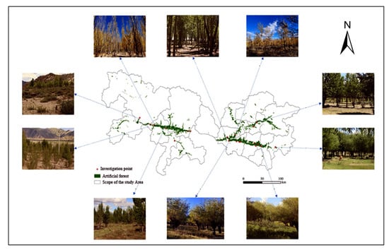
Figure 3.
The distribution of survey plots in the planted forests of the study area and corresponding field photos.
This research used ecosystem-type data from the soil conservation service module as input for the carbon module of the InVEST model, considering the wide range of natural ecosystems in the study region. Building upon the field survey of planted forests, and by thoroughly referencing local, field-measured soil carbon density data and carbon density parameters from the relevant literature on typical ecosystems of the Qingzang Plateau were utilized [24,25]. For every habitat in the research region, a thorough carbon density table was created and improved. Table 4 provides the relevant characteristics in detail.
Table 4.
Carbon density table of various ecosystems of YNL (Unit: t C/hm2).
- (4)
- Habitat Quality
A habitat quality index, which ranges from 0 to 1, is used in the InVEST model to reflect habitat quality; higher values indicate better habitat quality. The calculating formula is as follows:
where Hxj denotes the habitat appropriateness of land use type j and Qxj denotes the habitat quality of grid cell x in land use type j. Z is a normalization constant (often set to 2.5), k is the half-saturation constant (set to half the raster resolution, or 15), and Dxj is the overall danger level in grid cell x with land use type j.
where R is the total number of threat factors, r is a single threat factor, and y is a grid cell on the risk r raster. Yx represents the set of all grid cells on the raster. In grid cell y, ry is the danger r value (e.g., 0 or 1), irxy is the threat r impact from grid cell y on the habitat in grid cell x, and Wx n is the threat r weight (a number between 0 and 1). Sjx represents the sensitivity of habitat type j to threat factor r.
The habitat quality characteristics for the various ecosystems in the study region were thoroughly assessed and determined, using the InVEST model user’s manual and relevant research carried out in the Qingzang Plateau area [21,22] as a guide (Table 5 and Table 6).
Table 5.
Stress variables, maximum impact distance, and weight.
Table 6.
Habitat suitability and stress factor sensitivity.
2.3.2. Construction of the Comprehensive Ecosystem Service (CES) Index
This research used the InVEST model to quantitatively analyze four key ecosystem services in order to integrate the whole ecosystem functions within the study area: water conservation, carbon storage, soil conservation, and habitat quality. By merging these four services using an equal weighting and normalization mechanism, this research created a Comprehensive Ecosystem Service (CES) score to better comprehend their combined impacts [26,27]. The formulas are as follows:
CESj is the Comprehensive Ecosystem Service index for year j, φi is the weight of the i-th ecosystem service function, Sij is the normalized value of the i-th ecosystem service function in year j, n is the total number of ecosystem service types, Ei is the i-th ecosystem service function’s original value, and max Ei and min Ei are the i-th ecosystem service function’s maximum and minimum values, respectively.
2.3.3. Spatial Autocorrelation
To determine if there are clusters in a variable’s geographic distribution, spatial autocorrelation is used. Global and local autocorrelation are its two main applications. The former, represented by Moran’s I, correctly captures the general clustering features of the whole research region. The geographical distribution of these clusters may be mapped using the Local Indicators of geographical Association (LISA), which may provide an accurate representation of the clustering characteristics of local study units [28]. Whereas Local Moran’s I determines the spatial autocorrelation of a particular unit (or region), exposing local clustering tendencies, Global Moran’s I measures the spatial autocorrelation for the whole research area.
This study uses LISA to characterize the spatial autocorrelation between adjacent spatial units. First, a GIS platform was used to construct a 1 km × 1 km grid. Before beginning the study, a spatial weight matrix was created and the values of each ecosystem service were retrieved at the grid centers. LISA spatial clusters come in five varieties: Not Significant (areas that failed the significance test, p > 0.05), High–Low (a high value surrounded by low values), Low–High (a low value surrounded by high values), High–High (clusters of high values), and Low–Low (clusters of low values). The formulas are as follows:
where I, which has values between −1 and 1, is Global Moran’s I. Stronger clustering as it approaches one is indicated by a number greater than zero, while stronger dispersion as it approaches minus one is shown by a value less than zero. It is Local Moran’s I for region I, where n is the total number of units, ωij is the spatial weights matrix for units i and j, xi and xj are the observed values for spatial units i and j, and is the average value.
2.3.4. Principal Component Analysis (PCA)
PCA’s basic concept is to transform the original dataset’s variables into a new set of orthogonal variables, or principle components, which are then arranged according to how much of the original data’s variance they can account for. The first principal component explains the most possible variation, and each subsequent component explains the highest remaining variance, subject to the requirement that it is orthogonal to the previous components [29]. The factors under investigation in this study include eight independent variables (precipitation, temperature, elevation, aspect, slope, LUI, POP, and GDP) and one dependent variable, Comprehensive Ecosystem Services (CESs). The formula is as follows:
where y is the n × k transformation matrix, z is the matrix of k main components, and x is the matrix of n original variables.
2.3.5. Partial Least Squares Structural Equation Modeling (PLS-SEM) Analysis
The increasingly popular Partial Least Squares Structural Equation Modeling (PLS-SEM) method, which is usually used to model complex interactions between several variables at once, was used in this study. Compared to conventional covariance-based structural equation models (CB-SEMs), such those used in AMOS or LISREL, PLS-SEM is more flexible and is especially well suited for handling non-normal data and predictive research. The fields of business, marketing, management, social sciences, environmental research, and healthcare all make extensive use of PLS-SEM [30].
By building a system of variables (observed and latent) from a theoretical model, PLS-SEM calculates path coefficients. It can not only analyze direct relationships between variables but also assess mediating and moderating effects. It has the following advantages: (1) A core strength of PLS-SEM is its algorithm design, which blends principal component analysis with multiple regression’s advantages. Because of this, PLS-SEM is especially well suited for forecasting and elucidating intricate interactions [31]. This approach allows PLS-SEM to effectively extract the most important information when estimating complex models while maintaining the stability and interpretability of the model parameters. (2) PLS-SEM and CB-SEM differ primarily in that the former does not need the data to have a normal distribution. Furthermore, PLS-SEM necessitates minuscule sample sizes. (3) PLS-SEM is less stringent regarding model error and data assumptions, meaning it can work effectively even when data issues such as multicollinearity are present.
Using SmartPLS 4.0 software, the structural equation model was constructed in this study, and bootstrapping was used to assess the route coefficients’ relevance. The coefficient of determination (R2) is a standard metric for measuring model fit, used to explain how much the independent factors account for the variation in the dependent variable. A high R2 value in PLS-SEM means that the model does a good job of explaining the variation in the dependent variable [32,33] (Table 7).
Table 7.
PLS-SEM evaluation criteria.
3. Results
3.1. Temporal and Spatial Characteristics of Land Use
According to Table 8 and Figure 4, from 2000 to 2020, the areas of desert, shrubland, forest, and urban land exhibited an increasing trend, while grassland, glacier/permanent snow, cropland, and wetland showed a decreasing trend. The patterns of ecosystem area change varied across different time periods. Specifically, during 2000–2010, desert experienced the largest increase in area (+3698.71 km2), and desert showed the highest growth rate (+5.56%). In contrast, grassland had the largest decrease in area (−2652.45 km2). During 2010–2020, shrubland recorded the greatest increase in area (+2247.57 km2), and grassland had the highest decrease rate (−6.99%).
Table 8.
Land use type area change (km2) and change rate (%) in different periods.
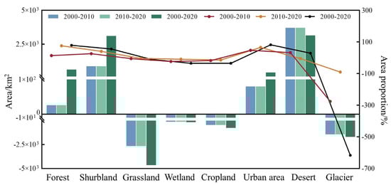
Figure 4.
Land use area change (km2) and change rate (%) in different periods from 2000 to 2020.
3.2. Spatiotemporal Characteristics of Ecosystem Services
3.2.1. Spatiotemporal Patterns of Ecosystem Services
The water conservation capacity of the studied region varies significantly by location and typically declines from east to west. The research area’s northwest region had the lowest levels of water conservation, while the northeastern and river valley areas had the greatest amounts (Figure 5). Between 2000 and 2020, both the average water conservation depth and the total water conservation volume exhibited an overall rising trend (Figure 6). The total water conservation volume increased by 253 million m3 (an increase of 1.87%, with an average rate of increase of 13 million m3/year), while the average water conservation depth increased by 3.43 mm. Between 2000 and 2010, the average water conservation depth in the study area rose by 0.34 mm, and the total volume increased by 26 million m3 (a 0.19% increase). Then, between 2010 and 2020, the total volume grew by 227 million m3 (a 1.40% increase) and the average water conservation depth increased by 3.09 mm.

Figure 5.
Spatial patterns of four essential ecosystem services, WC (a1,a2), SC (b1,b2), CS (c1,c2) and HQ (d1,d2), in the YNL area in 2000, 2010, and 2020.
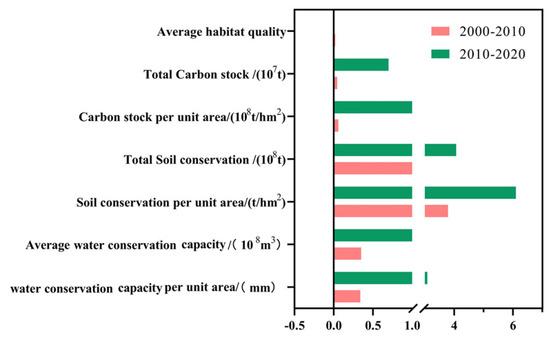
Figure 6.
Variation in ecosystem services across the study area from 2000 to 2020.
The amount of soil conservation in the study area increased overall between 2000 and 2020. Between 2000 and 2020, the average annual value increased from 37.24 t/(hm2·a) to 47.10 t/(hm2·a). The total volume increased from 246.79 million tons to 312.01 million tons, indicating a 26.43% rise (Figure 6). In terms of the distribution of space, the quantity of soil conservation generally exhibited a trend of being high in the east and low in the west, despite significant regional variations (Figure 5). Despite major regional variances, the study area’s total carbon storage changed very little between 2000 and 2020 (Figure 6), indicating a slight upward trend (Figure 5). The north-central portion of the research region saw a significant increase in carbon storage over the course of the 20 years. In contrast, carbon storage in the mountainous areas east of the Lhasa River exhibited a declining tendency. The research area’s total habitat quality showed a tendency of first declining and then rising between 2000 and 2020. With a mean value of 0.620 in 2000, habitat quality peaked, and in 2010, it fell to 0.608 on average. The average habitat quality dropped by 0.012 (a loss of 2.04%) between 2000 and 2010 and then climbed by 0.011 (a gain of 1.81%) between 2010 and 2020. Overall, the change in average habitat quality was minor, with variations occurring mainly at the regional level (Figure 5). Regions with good habitat quality were generally dispersed on both sides of the eastern river basins, corresponding to regions with a high coverage of shrublands and woods. Low-quality areas were predominantly found around bare lands in the west and in the vicinity of cultivated and constructed land.
3.2.2. Spatiotemporal Characteristics of Comprehensive Ecosystem Services (CESs)
In this study, the Comprehensive Ecosystem Services (CESs) in the study area exhibited pronounced spatiotemporal heterogeneity. Temporally, the average CES index showed a continuous upward trend from 2000 to 2020. Specifically, it increased by 2.77% during 2000–2010 and by 6.61% during 2010–2020, with a more substantial rise observed in the latter decade. This sustained improvement is likely associated with the implementation of national ecological protection policies, particularly the intensified efforts in ecological restoration and environmental governance during the most recent decade. Spatially, the CES index generally exhibited a declining pattern from east to west across the study area. The lowest CES values were found in the northwestern region, whereas higher values were concentrated in the northeastern part and the river valley plains (Figure 7).

Figure 7.
Spatiotemporal evolution of Comprehensive Ecosystem Services (CESs) from 2000 to 2020. Spatial Characteristics of Comprehensive Ecosystem Services for (a) 2000, (b) 2010, (c) 2020; (d) Temporal Variations of Comprehensive Ecosystem Services from 2000 to 2020.
3.2.3. Spatial Clustering Characteristics of Comprehensive Ecosystem Services
Significant geographical clustering characteristics were shown by the CES in all three time periods, with Global Moran’s I values of 0.7439 for 2000, 0.7759 for 2010, and 0.7306 for 2020, respectively (p < 0.01). This reveals a considerable positive geographical autocorrelation in the distribution of CESs, which means that places with high service values tend to cluster together, whereas those with poor service values also exhibit spatial clustering (Figure 8). Specifically, regarding the spatial clustering of CES in 2000, the “High–High” cluster type accounted for 17.41% of the area (Figure 8), primarily distributed in the eastern region. The “Low–Low” cluster type was most prevalent in the north-central region, making about 12.73% of the total area. The “High–Low” (0.40%) and “Low–High” (0.17%) outlier areas were minimal and showed a sporadic distribution. In 2010, the spatial clustering of CESs became more intensive. The “Low–Low” cluster type made up 14.84% of the area and was concentrated in the northwest, while the “High–High” cluster type made up 18.14% and was mostly dispersed in the eastern region (Figure 8). By 2020, the degree of spatial clustering of CESs had weakened. The “Low–Low” cluster type accounted for 14.13% of the area, with a dispersed distribution over the northwest and southern areas, whereas the “High–High” cluster type included 14.52% of the area, mostly in the eastern region (Figure 8).
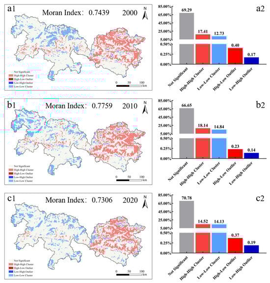
Figure 8.
Spatial clustering characteristics of Comprehensive Ecosystem Services (CESs). (a1,a2) Spatial Clustering Patterns in 2000 and the Proportion of Each Cluster Type; (b1,b2) Spatial Clustering Patterns in 2010 and the Proportion of Each Cluster Type; (c1,c2) Spatial Clustering Patterns in 2020 and the Proportion of Each Cluster Type.
3.3. Principal Component Analysis (PCA)
In order to separate the relationship between the Comprehensive Ecosystem Service (CES) index and a number of influencing factors, this study used Principal Component Analysis (PCA) to conduct an initial investigation of the relative effects of topographic factors (elevation, slope, and aspect), meteorological factors (precipitation and temperature), and human activities (GDP and POP) on CES change (Figure 9). Using PCA, eight parameters (one dependent variable, CESs, and seven independent variables) were decomposed into multiple principal component dimensions. The results showed that on the first principal component (PC1), which explained the most variance, the loading weights of the natural factors (elevation, temperature, and precipitation) were much higher than those of the human activity factors, with elevation having the largest absolute value. On the second principal component (PC2), the human activity factors (POP and GDP) had the highest loading weights. Since the variance explained by PC1 was significantly greater than that of PC2, the results of PC1 are more representative of the dominant driving forces. In conclusion, elevation, temperature, and precipitation are the main variables influencing the geographical distribution of Comprehensive Ecosystem Services (CESs), according to the exploratory analysis conducted using PCA.
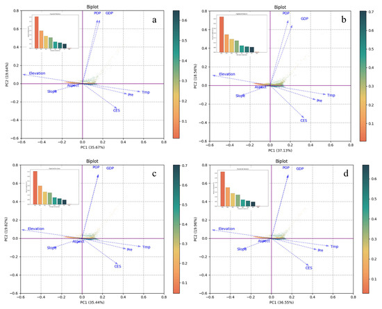
Figure 9.
Principal Component Analysis (PCA) results for the drivers of Comprehensive Ecosystem Services (CESs). The PCA biplot, which shows the relationship between each driving factor and CESs on the first (PC1) and second (PC2) principal components, is shown in the left panel. The right panel shows the percentage of variance that each principal component accounts for. Contribution of Various Driving Factors to Comprehensive Ecosystem Services for (a) 2000, (b) 2010, (c) 2020; (d) Contribution of Different Driving Factors to Multi-year Average Comprehensive Ecosystem Services.
3.4. PLS-SEM Analysis
The following theoretical presumptions were used in the construction of the Partial Least Squares Structural Equation Model (PLS-SEM): (1) Topographic variables impact climate patterns, which indirectly affect CESs; (2) patterns of natural factors (topography and climate) affect the extent of human activity; and (3) human activities may have a feedback effect on the local climate. To statistically examine these complicated causal pathways, our work used a PLS-SEM to explore the causes of CESs (Figure 10). The PLS-SEM had a decent overall goodness of fit based on model performance (Table 9).
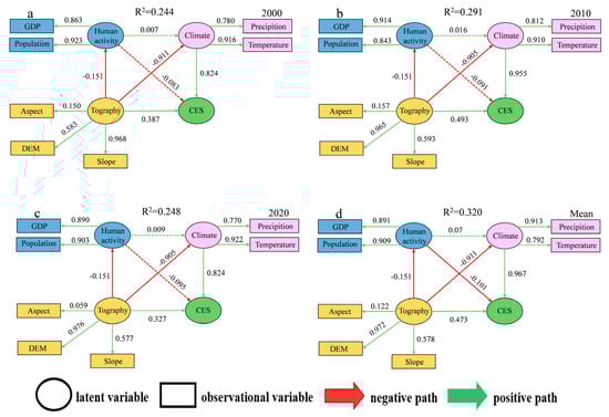
Figure 10.
Drivers of Comprehensive Ecosystem Services (CESs) are shown in the route diagram of the Partial Least Squares Structural Equation Model (PLS-SEM), Path coefficients above 0.1 are shown with solid lines, and those below 0.1 are shown with dashed lines. PLS-SEM Analysis of the Effects of Natural and Human Activity Factors on Comprehensive Ecosystem Services for (a) 2000, (b) 2010, (c) 2020; (d) PLS-SEM Analysis of the Effects of Natural and Human Activity Factors on Multi-year Average Comprehensive Ecosystem Services.
Table 9.
The performance of the PLS-SEM model.
Based on the path coefficient analysis, the interactions between the latent variables are as follows: With total impacts of 0.824, 0.955, and 0.778 for 2000, 2010, and 2020, respectively, the climatic component had the largest direct positive driving influence on CESs, making it the most important and direct factor affecting CES evolution. The topographic factor had a small direct impact on CESs but exerted a strong negative indirect effect primarily by affecting the climate (with indirect effects ranging from −0.905 to −0.911); its final total effect was positive (with total effects ranging from 0.327 to 0.493). This suggests that topography is a fundamental and foundational driver that determines the CES pattern. Human activities exhibited a weak negative overall effect on CESs (with total effects ranging from −0.083 to −0.095). However, their path coefficients and relative importance showed an increasing trend over time, reaching their strongest level in 2020, which reveals a growing potential threat.
4. Discussion
This study used an integrated approach that included the InVEST model, Principal Component Analysis (PCA), and Partial Least Squares Structural Equation Modeling (PLS-SEM) to quantitatively analyze the driving mechanisms of the spatiotemporal dynamics of ecosystem services in the YNL Basin of Xizang from 2000 to 2020. The main tenet of sustainable development and human well-being is ecosystem services [1]. Investigating their spatiotemporal evolution is crucial for solving regional ecological problems and maintaining ecological balance. A harmonious coexistence between humans and nature is facilitated when ecosystem services are taken into consideration while making decisions. The findings of this research provide important scientific insights for regional sustainable management in addition to explaining the evolutionary processes of this crucial and environmentally sensitive area.
4.1. Spatiotemporal Evolution Mechanisms of Ecosystem Services
Comprehensive Ecosystem Services (CESs) in the studied area showed a clear spatial differentiation pattern that was “high in the east and low in the west”. This pattern is in line with the region’s gradient distribution of natural geographical features. The Qingzang Plateau’s climate is mostly influenced by the East Asian monsoon. A macroscopic pattern of diminishing precipitation from southeast to northwest results from the Himalayan mountains’ blocking impact on the Indian monsoon and the westerlies [34,35]. The primary factor influencing the geographical distribution of alpine ecosystem services is the significant regional variance in hydrothermal conditions [36]. With woods and shrublands predominating the flora and a comparatively lower elevation, the eastern portion of the research area offers a greater natural basis for carbon sequestration, soil conservation, and water conservation services. In contrast, the western and northern regions are more arid, with vegetation consisting mostly of alpine grasslands, meadows, and deserts, resulting in a relatively weaker capacity for ecosystem service supply. This is in line with other studies on the Qingzang Plateau’s ecosystem services and Net Primary Productivity (NPP) [37].
Water conservation, soil conservation, and carbon storage services all saw increases from 2000 to 2020 on a temporal scale. This might be related to how human activities and climate change interact. On the one hand, the Qingzang Plateau is undergoing one of the world’s most dramatic “warming and wetting” processes, with a warming rate around double the worldwide average [38]. An overall increase in the Normalized Difference Plant Index (NDVI) [39] indicates that the increased temperature and precipitation in certain areas have boosted plant growth [40], which is a prerequisite for enhancing ecosystem services. However, China has implemented many important ecological conservation and restoration programs since the turn of the twenty-first century, such as the Grain for Green Program and the Natural Forest Protection Program, which have had favorable outcomes in the study region [41,42]. The field survey of carbon stocks in planted forests conducted in this study also indirectly confirms the contribution of ecological engineering to carbon sequestration capacity.
However, habitat quality first declined between 2000 and 2010 and then recovered, reflecting the complexity and dynamism of human impacts. The decrease in habitat quality prior to 2010 may be explained by the significant causes of habitat fragmentation and the degradation of ecosystem services, which include rapid urbanization and land use change [43,44,45]. Strengthening ecological protection laws and improving land use planning are probably responsible for the recovery that followed, showing that management measures may stop degradation trends and encourage human–nature coexistence [24].
4.2. Driving Role Analysis of Natural and Anthropogenic Factors
In order to identify the factors that contribute to CES change, this research used a two-step analytical approach known as “exploratory identification followed by causal validation.” First, the multidimensional driving factors’ dimensionality was reduced and their relevance was ranked using Principal Component Analysis (PCA), a useful technique often used in ecological research to pinpoint important explanatory variables [46,47]. The PCA findings clearly demonstrated that natural variables (particularly height, temperature, and precipitation) had much greater loading weights than other factors on the first principal component (PC1), which explained the majority of the overall variation. This discovery gave us guidance for later developing a more focused causal route model and enabled us to first determine the major factors influencing the spatial pattern of CES.
Therefore, this research used PLS-SEM to conduct a comprehensive causal path analysis. The advantages of multiple regression and Principle Component Analysis are combined in PLS-SEM, a powerful multivariate method that is appropriate for evaluating intricate networks of causal relationships in circumstances including multicollinearity between variables and non-normally distributed data [48]. The PLS-SEM analysis not only validated the exploratory findings of the PCA but also further quantified the direct and indirect pathways among the factors. The model indicated that climate factors (temperature and precipitation) are the strongest direct drivers of CESs in the study area. This result is consistent with a large body of research showing that the main constraints limiting plant growth and ecosystem function in alpine settings are hydro-thermal variables [49,50]. Topographic factors, in contrast, exert their dominant indirect effect mainly by regulating the distribution of water and heat [51]. For example, changes in elevation directly affect local patterns of precipitation and temperature, which in turn affect the types of plants and growth conditions, ultimately affecting the geographical distribution of ecosystem services.
Of high concern is that although the overall negative impact of current human activities (represented by GDP and population density) is relatively weak, its influence showed an increasing trend in 2020. This not only reveals the simple accumulation of anthropogenic pressure but, more critically, highlights the complex interaction mechanisms between climate change and human activities. These two factors do not act in isolation but rather influence the ecosystem jointly through synergistic or antagonistic effects [52]. This reveals a critical warning signal: as the economy develops in the plateau region, such as through the advancement of the Western Development Strategy [53] and population agglomeration, the pressure on the fragile ecosystem is rapidly accumulating.
Specifically, climate change can amplify the impacts of human activities. For instance, against the backdrop of climate warming, while vegetation greening driven by ecological engineering (a human activity) is inherently positive, the combined effect of both can lead to increased evapotranspiration, potentially “exacerbating water deficits” and posing a threat to regional water security [54]. Similarly, an interaction exists between climate warming and grazing activities, jointly affecting the net primary productivity of grasslands. This compounding effect of climate change and human activities collectively leads to “increased ecosystem sensitivity” [55], rendering it more vulnerable to future pressures.
Therefore, activities like road construction and urban expansion directly lead to habitat fragmentation and loss [56], while activities such as overgrazing cause grassland degradation and soil erosion [57]. If these activities are not effectively managed, their negative impacts are likely to be amplified in the future by the persistent “warming” trend [58,59], potentially offsetting some of the positive impacts brought by climate change and the protective achievements of ecological engineering, thereby threatening the region’s long-term ecological security [60]. This confirms the high sensitivity of the social–ecological relationship in this region, necessitating a more cautious balance between development and conservation [61].
4.3. Policy Implications and Management Suggestions
The findings of this research have important policy ramifications for the long-term growth and ecological preservation of the YNL Basin in Xizang as well as the larger Xi-zang plateau. To ensure that humans and the environment coexist peacefully, ecosystem services must be included into the decision-making process.
Given the spatial pattern of ecosystem services in the study area—characterized by higher values in the east and lower values in the west—as well as the evident spatial clustering of ecosystem functions, it is recommended that ecological management adopts a zonal strategy based on the principle of “prioritized conservation in high-value areas and focused restoration in low-value areas.” For “high–high” cluster regions with high ecosystem service functionality—particularly the eastern river valleys and forest–shrubland mosaics—these areas should be designated as core zones within ecological conservation redlines. The strictest protection measures should be implemented, such as restricting urban expansion, infrastructure development, and engineering disturbances, to ensure the stable provision of key ecological functions, including water conservation, soil conservation, and riparian biodiversity maintenance. Conversely, “low–low” cluster areas in the northwest with relatively weak ecological functions should be identified as priority zones for ecological restoration. Based on local topographic, climatic, and land use conditions, ecological projects such as afforestation and degraded grassland rehabilitation should be continuously promoted [62] to gradually enhance the region’s ecosystem service capacity.
For transitional areas between high and low ecosystem service values (“high-low” or “low-high” regions), it is necessary to explore pathways for the coordinated development of ecological conservation and local industry. This can include the implementation of ecological compensation mechanisms and the promotion of sustainable agriculture and pastoralism, aiming to improve both the efficiency of ecosystem service provision and the overall sustainability of regional development. Organize the Interaction between Economic Development and Ecological Security: Future infrastructure development, industrial layout, and urban design must all undergo thorough ecological and environmental impact evaluations due to the increasing strain from human activity. Because both urban and agricultural regions are dangerous, the land use structure should be modified to carefully control their chaotic expansion [28]. Furthermore, eco-friendly industries and sustainable livelihood models should be promoted to minimize the disturbance of development on the ecosystem [63,64].
Construct a Management Framework Based on Climate Change Adaptation: Since climate is a dominant driving factor, regional management policies must fully consider future climate change scenarios. The monitoring and prediction of the evolutionary trends of water resources, biodiversity, and ecosystem productivity under climate change should be strengthened. Based on this, ecological protection and restoration strategies should be dynamically adjusted to enhance the ecosystem’s adaptability and resilience to climate change [65].
4.4. Limitations and Prospects
This study still has several notable limitations. First, many of the biophysical parameters used in the InVEST model are derived from the previously published literature. Although some of these parameters were calibrated using field survey data, uncertainties remain due to the vast extent and high ecological heterogeneity of the study area. Such uncertainty is a common issue in the application of ecosystem models. Second, the construction of the Comprehensive Ecosystem Service (CES) index in this study adopts an equal weighting approach. While this method offers operational simplicity, it fails to account for the varying ecological significance and regional management priorities of different ecosystem services. In geographically complex and ecologically diverse landscapes, ecosystem services often exhibit significant non-linear interactions, including both synergies and trade-offs [66]. The equal weighting method may obscure the spatial heterogeneity and intricate interrelationships among services, thereby limiting a deeper understanding of multifunctional ecosystem dynamics [67]. Such an understanding is crucial for developing integrated and multi-objective ecosystem management strategies [27]. Third, in terms of the driver analysis, the PLS-SEM model employed in this study is a global model. While it effectively reveals the average impact of each driving factor across the entire study area, it does not capture the potential spatial heterogeneity of these effects. It must be emphasized that this was a deliberate choice based on data characteristics and model robustness. In the preliminary stages of our research, we attempted to use Geographically Weighted Regression (GWR) to explore these spatial variations. However, we encountered severe multicollinearity between key human activity indicators (GDP and POP), which caused the GWR model to fail due to “matrix is singular” errors, preventing the generation of stable and reliable results. Therefore, in the trade-off between the statistical robustness of our findings and the granularity of spatial detail, we prioritized the former.
Future studies might develop the following areas: First, by incorporating more localized, multi-scale field validations to further calibrate and optimize model parameters, assessment accuracy might be improved. Second, the results of the CES assessment could become more relevant to the region’s present socioeconomic development needs by objectively assigning weights to the various environmental services using techniques like factor analysis or the entropy weight approach. Third, by moving the study emphasis from integrated assessment to evaluating service interactions, important trade-offs and synergies, and driving processes, we may provide more precise evidence for ecological management choices. Fourth, to address the limitation of the global model in exploring spatial heterogeneity, future research could focus on exploring more advanced spatial analysis techniques, aiming to achieve an in-depth exploration of the spatial heterogeneity of driving factors while maintaining statistical robustness. Finally, we can contribute to the development of forward-looking adaptation methods by modeling and anticipating the long-term evolutionary tendencies of ecosystem services in the study area by merging future land use and climate change scenarios.
5. Conclusions
This research, which focused on the ecologically fragile YNL Basin in Xizang, revealed the spatiotemporal development features of its ecosystem services and their intricate driving mechanisms from 2000 to 2020 using an integrated analytical framework that combined the InVEST model and PCA-PLS-SEM.
According to the analysis, the ecosystem services in the study region have generally shown a positive trend over the past 20 years on a temporal scale. In particular, carbon storage, soil conservation, and water conservation have all steadily improved, and habitat quality has also recovered following a brief fluctuation. A clear scientific foundation for site-specific and zonally differentiated ecological management was provided by the Comprehensive Ecosystem Services (CESs), which continuously maintained a significant geographical differentiation of “high in the east and low in the west,” as well as strong spatial clustering between the high-value and low-value areas of these services.
At the level of driving mechanisms, this study confirms that natural factors are the fundamental force determining the current regional ecological pattern, with climate factors (temperature and precipitation) being the dominant direct drivers, while topography plays a key indirect regulatory role by influencing hydrothermal distribution. More importantly, this study quantitatively identified a core dynamic trend. Although the negative impact of human activities is not yet dominant overall, its relative influence is significantly increasing over time, highlighting the emerging challenge that development pressure poses to the ecosystem.
In conclusion, this study reveals that the ecosystem of the YNL Basin of Xizang is in a critical transitional period, characterized by the coexistence of positive recovery and potential risks. The two main factors affecting its development are human activity and climate change. Future management plans for this area must thus move beyond static, one-dimensional conservation objectives. Establishing an integrated ecological management paradigm that is based on spatial heterogeneity, actively coordinates conflicts between development and conservation, and can pro-actively adapt to climate change is essential to ensuring the long-term viability of this nationally significant ecological security barrier.
Author Contributions
Conceptualization, C.S., J.L., S.Y. and Z.W.; methodology, C.S. and Z.W.; software, Z.W. and S.Y.; validation, Z.W., H.W. and D.Y.; formal analysis, C.S., Z.W. and H.W.; investigation, Z.W.; resources, Z.W., P.P. and H.O.; data curation, C.S., Z.W., S.Y. and H.W.; writing—original draft preparation, Z.W., S.Y. and X.T.; writing—review and editing, J.L., X.T., L.C. and P.P.; visualization, Z.W., J.L. and S.Y.; supervision, J.L. and P.P.; project administration, J.L.; funding acquisition, J.L. All authors have read and agreed to the published version of the manuscript.
Funding
The National Key R&D Program of China (2024YFF1307800, 2024YFF1307804); Major Science and Technology Special Projects of Tibet Autonomous Region (XZ202201ZD0005G03); Base and Talent Project of Xizang (XZ202401JD0003); and Ongoing Engineering Project in Tibet of Huaneng, China (JC2022/D01).
Data Availability Statement
The data used to support the findings of this study are available from the corresponding author upon request.
Acknowledgments
We are grateful to NASA (https://earthexplorer.usgs.gov/), the National Tibetan Plateau/Third Pole Environment Data Center (https://data.tpdc.ac.cn/), the Resource and Environment Science and Data Center (https://www.resdc.cn/), and the Geospatial Data Cloud (https://www.gscloud.cn/) for providing original datasets. We appreciate the anonymous reviewers for providing invaluable comments on the original manuscript.
Conflicts of Interest
Authors Dong Yan and Haijun Ouyang was employed by the company Huaneng Tibet YarlungZangbo River Hydropower Development Investment Co., Ltd. The remaining authors declare that the research was conducted in the absence of any commercial or financial relationships that could be construed as a potential conflict of interest.
References
- Drupp, M.A.; Haensel, M.C.; Fenichel, E.P.; Freeman, M.; Gollier, C.; Groom, B.; Heal, G.M.; Howard, P.H.; Millner, A.; Moore, F.C.; et al. Accounting for the increasing benefits from scarce ecosystems. Science 2024, 383, 1062–1064. [Google Scholar] [CrossRef]
- Daily, G.C. Nature’s Services: Societal Dependence on Natural Ecosystems; Island Press: Washington, DC, USA, 1997. [Google Scholar]
- Costanza, R.; d’Arge, R.; De Groot, R.; Farber, S.; Grasso, M.; Hannon, B.; Limburg, K.; Naeem, S.; O’neill, R.V.; Paruelo, J.; et al. The value of the world’s ecosystem services and natural capital. Nature 1997, 387, 253–260. [Google Scholar] [CrossRef]
- Pang, D.Y.; Zhao, M.Y.; Cai, L.P.; Xu, Y.L.; Zhang, W.E. The trade-offs effect of ecosystem health and socio-economic development on tea production. Ecol. Indic. 2024, 166, 112416. [Google Scholar] [CrossRef]
- Dai, X.; Wang, L.C.; Huang, C.B.; Fang, L.L.; Wang, S.Q.; Wang, L.Z. Spatio-temporal variations of ecosystem services in the urban agglomerations in the middle reaches of the Yangtze River, China. Ecol. Indic. 2020, 115, 106394. [Google Scholar] [CrossRef]
- Awuah, K.F.; Jegede, O.; Hale, B.; Siciliano, S.D. Introducing the Adverse Ecosystem Service Pathway as a Tool in Ecological Risk Assessment. Environ. Sci. Technol. 2020, 54, 8144–8157. [Google Scholar] [CrossRef]
- Larondelle, N.; Lauf, S. Balancing demand and supply of multiple urban ecosystem services on different spatial scales. Ecosyst. Serv. 2016, 22, 18–31. [Google Scholar] [CrossRef]
- Vihervaara, P.; Rönkä, M.; Walls, M. Trends in Ecosystem Service Research: Early Steps and Current Drivers. Ambio 2010, 39, 314–324. [Google Scholar] [CrossRef] [PubMed]
- An, Z.Y.; Sun, C.Z.; Hao, S. Exploration of ecological compensation standard: Based on ecosystem service flow path. Appl. Geogr. 2025, 178, 103588. [Google Scholar] [CrossRef]
- Bennett, E.M.; Peterson, G.D.; Gordon, L.J. Understanding relationships among multiple ecosystem services. Ecol. Lett. 2009, 12, 1394–1404. [Google Scholar] [CrossRef]
- Haines-Young, R.; Potschin, M. The links between biodiversity, ecosystem services and human well-being. In Ecosystem Ecology: A New Synthesis; Raffaelli, D.G., Frid, C.L.J., Eds.; Cambridge University Press: Cambridge, UK, 2010; pp. 110–139. [Google Scholar]
- Sun, X.Y.; Shan, R.F.; Liu, F. Spatio-temporal quantification of patterns, trade-offs and synergies among multiple hydrological ecosystem services in different topographic basins. J. Clean. Prod. 2020, 268, 122338. [Google Scholar] [CrossRef]
- Kim, J.H.; Jobbÿgy, E.G.; Jackson, R.B. Trade-offs in water and carbon ecosystem services with land-use changes in grasslands. Ecol. Appl. 2016, 26, 1633–1644. [Google Scholar] [CrossRef]
- Che, L.; Guo, S.D.; Li, Y.L. Discerning changes and drivers of water yield ecosystem service: A case study of Chongqing-Chengdu District, Southwest China. Ecol. Indic. 2024, 160, 111767. [Google Scholar] [CrossRef]
- Sang, H.B.; Liu, Y.; Sun, Z.X.; Han, W.Y. Three-dimensional analysis and drivers of relationships among multiple ecosystem services: A case study in the Nansi Lake Basin, China. Environ. Impact Assess. Rev. 2024, 106, 107521. [Google Scholar] [CrossRef]
- Wang, B.; Hu, C.G.; Zhang, Y.S. Multi-Scenario Simulation of the Impact of Land Use Change on the Ecosystem Service Value in the Suzhou-Wuxi-Changzhou Metropolitan Area, China. Chin. Geogr. Sci. 2024, 34, 79–92. [Google Scholar] [CrossRef]
- Balvanera, P.; Pfisterer, A.B.; Buchmann, N.; He, J.S.; Nakashizuka, T.; Raffaelli, D.; Schmid, B. Quantifying the evidence for biodiversity effects on ecosystem functioning and services. Ecol. Lett. 2006, 9, 1146–1156. [Google Scholar] [CrossRef] [PubMed]
- Braun, D.; de Jong, R.; Schaepman, M.E.; Furrer, R.; Hein, L.; Kienast, F.; Damm, A. Ecosystem service change caused by climatological and non-climatological drivers: A Swiss case study. Ecol. Appl. 2019, 29, e01901. [Google Scholar] [CrossRef]
- Liu, H.; Deng, Y.; Liu, X.Q. The contribution of forest and grassland change was greater than that of cropland in human-induced vegetation greening in China, especially in regions with high climate variability. Sci. Total Environ. 2021, 792, 148408. [Google Scholar] [CrossRef] [PubMed]
- Sun, W.Y.; Shao, Q.Q.; Liu, J.Y.; Zhai, J. Assessing the effects of land use and topography on soil erosion on the Loess Plateau in China. Catena 2014, 121, 151–163. [Google Scholar] [CrossRef]
- Natural Capital Project, 2025. InVEST 3.16.2. Stanford University, University of Minnesota, Chinese Academy of Sciences, The Nature Conservancy, World Wildlife Fund, Stockholm Resilience Centre and the Royal Swedish Academy of Sciences. Available online: https://natcap.github.io/invest.release-metadata/3.16.2.html (accessed on 10 December 2024).
- Jia, Z.X.; Wang, X.F.; Feng, X.M.; Ma, J.H.; Wang, X.X.; Zhang, X.R.; Zhou, J.T.; Sun, Z.C.; Yao, W.J.; Tu, Y. Exploring the spatial heterogeneity of ecosystem services and influencing factors on the Qinghai Tibet Plateau. Ecol. Indic. 2023, 154, 110521. [Google Scholar] [CrossRef]
- Haq, S.M.; Rashid, I.; Calixto, E.S.; Ali, A.; Kumar, M.; Srivastava, G.; Bussmann, R.W.; Khuroo, A.A. Unravelling patterns of forest carbon stock along a wide elevational gradient in the Himalaya: Implications for climate change mitigation. For. Ecol. Manag. 2022, 521, 120442. [Google Scholar] [CrossRef]
- Wang, Z.Y.; Song, W.; Yin, L.C. Responses in ecosystem services to projected land cover changes on the Tibetan Plateau. Ecol. Indic. 2022, 142, 109228. [Google Scholar] [CrossRef]
- Liu, H.; Liu, S.L.; Wang, F.F.; Liu, Y.X.; Liu, Y.X.; Sun, J.; McConkey, K.R.; Tran, L.S.P.; Dong, Y.H.; Yu, L.; et al. Identifying ecological compensation areas for ecosystem services degradation on the Qinghai-Tibet Plateau. J. Clean. Prod. 2023, 423, 138626. [Google Scholar] [CrossRef]
- Gong, D.H.; Dong, D.J.; Du, H.Q.; Zhou, Y.F.; Fu, S.; Fujioka, Y. Spatiotemporal coupling mechanisms and driving forces of ecosystem services and human activity from a multidimensional perspective. Int. J. Digit. Earth 2025, 18, 2512061. [Google Scholar] [CrossRef]
- Wu, L.L.; Fan, F.L. Assessment of ecosystem services in new perspective: A comprehensive ecosystem service index (CESI) as a proxy to integrate multiple ecosystem services. Ecol. Indic. 2022, 138, 108800. [Google Scholar] [CrossRef]
- Peng, Y.L.; Chen, W.X.; Pan, S.P.; Gu, T.C.; Zeng, J. Identifying the driving forces of global ecosystem services balance, 2000–2020. J. Clean. Prod. 2023, 426, 139019. [Google Scholar] [CrossRef]
- Mahmoudi, M.R.; Heydari, M.H.; Qasem, S.N.; Mosavi, A.; Band, S.S. Principal component analysis to study the relations between the spread rates of COVID-19 in high risks countries. Alex. Eng. J. 2021, 60, 457–464. [Google Scholar] [CrossRef]
- Akter, S.; Wamba, S.F.; Dewan, S. Why PLS-SEM is suitable for complex modelling? An empirical illustration in big data analytics quality. Prod. Plan. Control 2017, 28, 1011–1021. [Google Scholar] [CrossRef]
- Sarstedt, M.; Ringle, C.M.; Cheah, J.H.; Ting, H.R.; Moisescu, O.; Radomir, L. Structural model robustness checks in PLS-SEM. Tour. Econ. 2020, 26, 531–554. [Google Scholar] [CrossRef]
- Chin, W.; Cheah, J.H.; Liu, Y.D.; Ting, H.; Lim, X.J.; Cham, T.H. Demystifying the role of causal-predictive modeling using partial least squares structural equation modeling in information systems research. Ind. Manag. Data Syst. 2020, 120, 2161–2209. [Google Scholar] [CrossRef]
- Hair, J.F.; Sarstedt, M. Factors versus Composites: Guidelines for Choosing the Right Structural Equation Modeling Method. Proj. Manag. J. 2019, 50, 619–624. [Google Scholar] [CrossRef]
- Yao, T.D.; Masson-Delmotte, V.; Gao, J.; Yu, W.S.; Yang, X.X.; Risi, C.; Sturm, C.; Werner, M.; Zhao, H.B.; He, Y.; et al. A Review of Climatic Controls on Δ18o in Precipitation Over the Tibetan Plateau: Observations and Simulations. Rev. Geophys. 2013, 51, 525–548. [Google Scholar] [CrossRef]
- Gao, J.; Yao, T.D.; Masson-Delmotte, V.; Steen-Larsen, H.C.; Wang, W.C. Collapsing glaciers threaten Asia’s water supplies. Nature 2019, 565, 19–21. [Google Scholar] [CrossRef]
- Zhang, T.; Zhang, Y.J.; Xu, M.J.; Zhu, J.T.; Chen, N.; Jiang, Y.B.; Huang, K.; Zu, J.X.; Liu, Y.J.; Yu, G.R. Water availability is more important than temperature in driving the carbon fluxes of an alpine meadow on the Tibetan Plateau. Agric. For. Meteorol. 2018, 256, 22–31. [Google Scholar] [CrossRef]
- Ma, S.; Wang, L.J.; Jiang, J.; Chu, L.; Zhang, J.C. Threshold effect of ecosystem services in response to climate change and vegetation coverage change in the Qinghai-Tibet Plateau ecological shelter. J. Clean. Prod. 2021, 318, 128592. [Google Scholar] [CrossRef]
- Guo, D.L.; Wang, H.J. The significant climate warming in the northern Tibetan Plateau and its possible causes. Int. J. Climatol. 2012, 32, 1775–1781. [Google Scholar] [CrossRef]
- Li, P.L.; Zhu, D.; Wang, Y.L.; Liu, D. Elevation dependence of drought legacy effects on vegetation greenness over the Tibetan Plateau. Agric. For. Meteorol. 2020, 295, 108190. [Google Scholar] [CrossRef]
- Xu, B.N.; Li, J.J.; Pei, X.J.; Yang, H.L. Decoupling the response of vegetation dynamics to asymmetric warming over the Qinghai-Tibet plateau from 2001 to 2020. J. Environ. Manag. 2023, 347, 119131. [Google Scholar] [CrossRef] [PubMed]
- Mengist, W.; Soromessa, T.; Feyisa, G.L. Responses of carbon sequestration service for landscape dynamics in the Kaffa biosphere reserve, southwest Ethiopia. Environ. Impact Assess. Rev. 2023, 98, 106960. [Google Scholar] [CrossRef]
- Xu, B.N.; Li, J.J.; Pei, X.J.; Bian, L.J.; Zhang, T.B.; Yi, G.H.; Bie, X.J.; Peng, P.H. Dominance of Topography on Vegetation Dynamics in the Mt. Qomolangma National Nature Reserve: A UMAP and PLS-SEM Analysis. Forests 2023, 14, 1415. [Google Scholar] [CrossRef]
- Xiao, R.; Lin, M.; Fei, X.F.; Li, Y.S.; Zhang, Z.H.; Meng, Q.X. Exploring the interactive coercing relationship between urbanization and ecosystem service value in the Shanghai-Hangzhou Bay Metropolitan Region. J. Clean. Prod. 2020, 253, 119803. [Google Scholar] [CrossRef]
- Shi, Y.; Feng, C.C.; Yu, Q.R.; Han, R.; Guo, L. Contradiction or coordination? The spatiotemporal relationship between landscape ecological risks and urbanization from coupling perspectives in China. J. Clean. Prod. 2022, 363, 132557. [Google Scholar] [CrossRef]
- Lyu, R.F.; Clarke, K.C.; Zhang, J.M.; Feng, J.L.; Jia, X.H.; Li, J.J. Spatial correlations among ecosystem services and their socio-ecological driving factors: A case study in the city belt along the Yellow River in Ningxia, China. Appl. Geogr. 2019, 108, 64–73. [Google Scholar] [CrossRef]
- Xu, B.N.; Li, J.J.; Liu, Y.G.; Zhang, T.B.; Luo, Z.Y.; Pei, X.J. Disentangling the response of vegetation dynamics to natural and anthropogenic drivers over the Qinghai-Tibet Plateau using dimensionality reduction and structural equation model. For. Ecol. Manag. 2024, 554, 121677. [Google Scholar] [CrossRef]
- Kang, Y.J.; Wang, Z.Q.; Xu, B.N.; Shen, W.J.; Chen, Y.; Zhou, X.H.; Liu, Y.G.; Zhang, T.B.; Wang, G.Y.; Jia, Y.L.; et al. Disentangling the Response of Vegetation Dynamics to Natural and Anthropogenic Drivers over the Minjiang River Basin Using Dimensionality Reduction and a Structural Equation Model. Forests 2024, 15, 1438. [Google Scholar] [CrossRef]
- Hair, J.F., Jr.; Ringle, C.M.; Sarstedt, M. Partial Least Squares Structural Equation Modeling: Rigorous Applications, Better Results and Higher Acceptance. Long. Range Plan. 2013, 46, 1–12. [Google Scholar] [CrossRef]
- Zhang, C.; Lu, D.S.; Chen, X.; Zhang, Y.M.; Maisupova, B.; Tao, Y. The spatiotemporal patterns of vegetation coverage and biomass of the temperate deserts in Central Asia and their relationships with climate controls. Remote Sens. Environ. 2016, 175, 271–281. [Google Scholar] [CrossRef]
- Piao, S.L.; Yin, G.D.; Tan, J.G.; Cheng, L.; Huang, M.T.; Li, Y.; Liu, R.G.; Mao, J.F.; Myneni, R.B.; Peng, S.S.; et al. Detection and attribution of vegetation greening trend in China over the last 30 years. Glob. Change Biol. 2015, 21, 1601–1609. [Google Scholar] [CrossRef]
- Shen, M.G.; Piao, S.L.; Jeong, S.J.; Zhou, L.M.; Zeng, Z.Z.; Ciais, P.; Chen, D.L.; Huang, M.T.; Jin, C.S.; Li, L.Z.X.; et al. Evaporative cooling over the Tibetan Plateau induced by vegetation growth. Proc. Natl. Acad. Sci. USA 2015, 112, 9299–9304. [Google Scholar] [CrossRef]
- Wang, Y.; Lv, W.; Xue, K.; Wang, S.; Zhang, L.; Hu, R.; Zeng, H.; Xu, X.; Li, Y.; Jiang, L.; et al. Grassland changes and adaptive management on the Qinghai—Tibetan Plateau. Nat. Rev. Earth Environ. 2022, 3, 668–683. [Google Scholar] [CrossRef]
- Zhang, T.Q.; Yu, W.B.; Lu, Y.; Chen, L. Identification and Correlation Analysis of Engineering Environmental Risk Factors along the Qinghai-Tibet Engineering Corridor. Remote Sens. 2022, 14, 908. [Google Scholar] [CrossRef]
- Liu, J.; Milne, R.I.; Cadotte, M.W.; Wu, Z.Y.; Provan, J.; Zhu, G.F.; Gao, L.M.; Li, D.Z. Protect Third Pole’s fragile ecosystem. Science 2018, 362, 1368. [Google Scholar] [CrossRef]
- Fan, K.; Zhang, Q.; Singh, V.P.; Sun, P.; Song, C.; Zhu, X.; Yu, H.; Shen, Z. Spatiotemporal impact of soil moisture on air temperature across the Tibet Plateau. Sci. Total Environ. 2019, 649, 1338–1348. [Google Scholar] [CrossRef] [PubMed]
- Li, W.; Kang, J.; Wang, Y. Exploring the interactions and driving factors among typical ecological risks based on ecosystem services: A case study in the Sichuan-Yunnan ecological barrier area. Ecol. Indic. 2025, 170, 113000. [Google Scholar] [CrossRef]
- Newbold, T.; Hudson, L.N.; Hill, S.L.L.; Contu, S.; Lysenko, I.; Senior, R.A.; Börger, L.; Bennett, D.J.; Choimes, A.; Collen, B.; et al. Global effects of land use on local terrestrial biodiversity. Nature 2015, 520, 45. [Google Scholar] [CrossRef]
- Yin, X.; Wu, Y.; Zhao, W.; Liu, S.; Zhao, F.; Chen, J.; Qiu, L.; Wang, W. Spatiotemporal responses of net primary productivity of alpine ecosystems to flash drought: The Qilian Mountains. J. Hydrol. 2023, 624, 129865. [Google Scholar] [CrossRef]
- Xu, B.N.; Li, J.J.; Luo, Z.Y.; Wu, J.H.; Liu, Y.G.; Yang, H.L.; Pei, X.J. Analyzing the Spatiotemporal Vegetation Dynamics and Their Responses to Climate Change along the Ya’an-Linzhi Section of the Sichuan-Tibet Railway. Remote Sens. 2022, 14, 3584. [Google Scholar] [CrossRef]
- Su, D.; Cao, Y.; Dong, X.Y.; Wu, Q.; Fang, X.Q.; Cao, Y. Evaluation of ecosystem services budget based on ecosystem services flow: A case study of Hangzhou Bay area. Appl. Geogr. 2024, 162, 103150. [Google Scholar] [CrossRef]
- Jiang, W.; Lü, Y.H.; Liu, Y.X.; Gao, W.W. Ecosystem service value of the Qinghai-Tibet Plateau significantly increased during 25 years. Ecosyst. Serv. 2020, 44, 101146. [Google Scholar] [CrossRef]
- Hua, F.Y.; Wang, X.Y.; Zheng, X.L.; Fisher, B.; Wang, L.; Zhu, J.G.; Tang, Y.; Yu, D.W.; Wilcove, D.S. Opportunities for biodiversity gains under the world’s largest reforestation programme. Nat. Commun. 2016, 7, 12717. [Google Scholar] [CrossRef] [PubMed]
- Ouyang, Z.Y.; Song, C.S.; Zheng, H.; Polasky, S.; Xiao, Y.; Bateman, I.J.; Liu, J.G.; Ruckelshaus, M.; Shi, F.Q.; Xiao, Y.; et al. Using gross ecosystem product (GEP) to value nature in decision making. Proc. Natl. Acad. Sci. USA 2020, 117, 14593–14601. [Google Scholar] [CrossRef]
- Wright, W.C.C.; Eppink, F.V.; Greenhalgh, S. Are ecosystem service studies presenting the right information for decision making? Ecosyst. Serv. 2017, 25, 128–139. [Google Scholar] [CrossRef]
- Dong, K.; Wang, S.N.; Hu, H.Q.; Guan, N.N.; Shi, X.L.; Song, Y. Financial development, carbon dioxide emissions, and sustainable development. Sustain. Dev. 2024, 32, 348–366. [Google Scholar] [CrossRef]
- Zhao, T.; Pan, J.; Bi, F. Can human activities enhance the trade-off intensity of ecosystem services in arid inland river basins? Taking the Taolai River asin as an example. Sci. Total Environ. 2023, 861, 160662. [Google Scholar] [CrossRef] [PubMed]
- Liu, Z.Y.; Zhang, P.Y.; Li, G.H.; Yang, D.; Qin, M.Z. The Response of Composite Ecosystem Services to Urbanization: From the Perspective of Spatial Relevance and Spatial Spillover. IEEE J. Sel. Top. Appl. Earth Obs. Remote Sens. 2023, 16, 8204–8214. [Google Scholar] [CrossRef]


Disclaimer/Publisher’s Note: The statements, opinions and data contained in all publications are solely those of the individual author(s) and contributor(s) and not of MDPI and/or the editor(s). MDPI and/or the editor(s) disclaim responsibility for any injury to people or property resulting from any ideas, methods, instructions or products referred to in the content. |
© 2025 by the authors. Licensee MDPI, Basel, Switzerland. This article is an open access article distributed under the terms and conditions of the Creative Commons Attribution (CC BY) license (https://creativecommons.org/licenses/by/4.0/).