Abstract
Surface solar irradiance (SSI) is a critical factor influencing the power generation capacity of photovoltaic (PV) power plants. Dynamic changes in cloud cover pose significant challenges to the accurate nowcasting of SSI, which in turn directly affects the reliability and stability of renewable energy systems. However, existing research often simplifies or overlooks changes in the optical and morphological characteristics of clouds, leading to considerable errors in SSI nowcasting. To address this limitation and improve the accuracy of ultra-short-term SSI forecasting, this study first forecasts changes in cloud optical thickness (COT) within the next 3 h based on a spatiotemporal long short-term memory model, since COT is the primary factor determining cloud shading effects, and then integrates the zenith and regional averages of COT, along with factors influencing direct solar radiation and scattered radiation, to achieve precise SSI nowcasting. To validate the proposed method, we apply it to the Albuquerque, New Mexico, United States (ABQ) site, where it yielded promising performance, with correlations between predicted and actual surface solar irradiance for the next 1 h, 2 h, and 3 h reaching 0.94, 0.92, and 0.92, respectively. The proposed method effectively captures the temporal trends and spatial patterns of cloud changes, avoiding simplifications of cloud movement trends or interference from non-cloud factors, thus providing a basis for power adjustments in solar power plants.
1. Introduction
Global warming has emerged as a critical environmental crisis. Data released by NASA’s Goddard Institute for Space Studies (GISS) in November 2024 revealed that global monthly average temperatures have been 0.3 to 0.5 °C higher than historical records since June 2023, mainly due to greenhouse gas emissions from human activities [1]. Within the energy sector, electricity generation and consumption represent significant sources of these emissions. According to the International Energy Agency (IEA), fossil fuels still dominate the global electricity mix, accounting for approximately 54% in 2024 [2], while renewable energy sources have gradually increased their share to 38%, driven by growing concerns regarding climate change. Among them, solar energy, as a representative clean energy source, can be efficiently converted into electricity through photovoltaic (PV) technology. Therefore, photovoltaic systems are widely deployed worldwide [3,4]. However, their power output can be irregular and fluctuate due to the intermittent nature of surface solar irradiance (SSI) caused by factors such as cloud cover and seasonal and intraday variations. These fluctuations introduce challenges to power system stability and grid management [5,6,7,8,9]. Accurate short-term SSI forecasting, or nowcasting, is thus crucial for optimizing grid operations and enabling large-scale solar energy deployment.
Over the past two decades, extensive research efforts have been devoted to solar irradiance and PV power generation nowcasting [3,4], employing three primary approaches: physical methods, traditional statistical methods, and machine learning-based methods [10]. Physical methods model solar irradiance prediction by utilizing numerical weather prediction (NWP) and cloud maps [11]; however, they encounter challenges including estimation uncertainties [12], computational complexity, large parameter requirements [13], and limited forecasting accuracy [14]. Traditional statistical methods relying on curve fitting and correlation analysis of historical data [15] are valued for their simplicity and generalizability. Nevertheless, they often struggle with accuracy during rapid weather changes [16], and the extensive calculations required often prove too time-consuming to satisfy the accuracy and speed demands of ultra-short-term solar irradiance or PV power forecasts [17]. Machine learning-based methods, including artificial neural networks [18,19], random forests [20,21], and support vector machines [22], demonstrated significant potential for short-term solar irradiance forecasting due to their capacity to capture nonlinear relationships and temporal trends within historical data [23]. When focusing on ultra-short-term solar irradiance forecasting, cloud movement and dissipation are two critical factors. Cloud images provide valuable information on cloud shape, transparency, and distribution, revealing hidden spatiotemporal relationships. Current forecasting methods based on cloud images are mainly categorized into two types: those using ground-based all-sky imagers (TSI) and those relying on satellite imagery. TSIs offer high spatiotemporal resolution [24,25,26], but their utility is constrained by limited monitoring range coupled with high installation and maintenance costs. In contrast, satellite imagery provides wider coverage, diverse data sources, and better monitoring of cloud changes, making it more suitable for large-scale solar irradiance and PV power forecasting.
Recent studies have demonstrated various approaches to satellite-based solar irradiance nowcasting, which typically proceeds in two stages: first, a model predicts the spatiotemporal evolution of clouds, and second, the predicted cloud field is converted to surface radiation either via a physical formulation or a machine-learning regressor. For cloud-motion forecasting, traditional approaches rely on block-matching and feature-based linear extrapolation, which locate salient image features and track them to derive cloud-motion vectors. These methods, however, assume homogeneous advection and can incur large errors when wind fields vary or viewing geometry changes. Subsequently, optical flow techniques have been adopted to estimate cloud motion; for example, Kosmopoulos et al. [27] used near-real-time satellite cloud data with two methods (Farnebäck and TV-L1) to predict cloud movement and compute surface radiation for large-scale regions. More recently, deep learning has gained prominence: Si et al. [28] used satellite-visible cloud images and convolutional long short-term memory networks (ConvLSTM) to forecast cloud movement, combined with physical deduction and the XGBoost model to predict PV power. Straub et al. [29] introduced HelioNet, a UNet-based convolutional neural network, to predict future cloud index situations from sequences of preceding cloud index images, aiming to replace conventional cloud-motion vectors (CMVs) in satellite-based solar irradiance forecasting. Compared with optical flow techniques, deep-learning approaches excel at capturing nonlinear cloud motion and cloud formation/decay, features critical for accurate cloud forecasting and, by extension, reliable surface-radiation nowcasting. Despite these advances, several limitations persist in satellite-based solar irradiance nowcasting. First, both the temporal and spatial precision of forecast results require further improvement. Then, current studies rarely quantify cloud shading effects on solar radiation using detailed cloud attributes, resulting in limited modeling accuracy. Cloud optical thickness (COT) is a pivotal physical parameter that directly modulates the attenuation of solar radiation reaching the Earth’s surface [30]. The larger the COT value, the more pronounced the attenuation effect, thereby significantly influencing the accuracy of solar radiation estimation. COT also alters the balance between direct and scattered radiation: thin clouds tend to enhance scattering, while thick clouds suppress total radiation. Additionally, COT impacts the error sensitivity of radiation nowcasting, with errors in thin-cloud scenarios having a more substantial influence. Given these multifaceted roles, COT is crucial in determining both the total amount and spatial distribution of solar radiation and is a key determinant of nowcasting precision for surface solar radiation.
In this study, we propose an innovative method to enhance SSI nowcasting through COT utilization. Specifically, we first employ a spatiotemporal long short-term memory network model (PredRNN) [31] to forecast COT images with a 2-km spatial resolution and 15-min intervals for the next 3 h. These satellite COT images serve as the primary basis for solar radiation nowcasting. The inclusion of nighttime COT products expands the training dataset, while the COT images themselves provide more accurate representations of cloud attenuation effects compared to conventional visible light images. By optimizing the PredRNN model, we effectively address cloud deformation and movement, achieving precise 3-h COT forecasts. In the second stage, we employ the LightGBM model to estimate SSI for the next 1 h, 2 h, and 3 h at a specific site. To validate our methodology, we conduct comprehensive testing at the Albuquerque, New Mexico, United States (ABQ) site, where we perform detailed comparisons between predicted and observed SSI values across the next 3 h. This validation framework is designed to support accurate photovoltaic power prediction in practical applications.
2. Materials and Methods
2.1. Datasets
The dataset employed in this study primarily falls into two categories: one is geostationary satellite-derived COT products for predicting COT values at target sites and their adjacent regions, and the other is ground-based observational measurements of surface solar irradiance utilized for SSI estimation and prediction.
2.1.1. Cloud Optical Thickness Data
The COT data used in this study were obtained from the Advanced Baseline Imager (ABI) sensor aboard the United States geostationary satellite GOES-16 (operated by National Aeronautics and Space Administration (Washington, DC, USA) and National Oceanic and Atmospheric Administration (Silver Spring, MD, USA)), specifically utilizing its Level2 (L2) scientific product containing observations from the 0.64 μm and 2.25 μm spectral bands (https://www.aev.class.noaa.gov/saa/products/search?datatype_family=GRABIPRD (accessed on 25 October 2024)). The COT dataset quantifies cloud extinction coefficients at λ = 0.64 μm through per-pixel measurements of hydrometeor attenuation characteristics for both liquid and ice cloud phases [32].
The study utilizes two types of COT products: daytime and nighttime. Daytime COT data has a measurement range of 0–160, performs well within Local Zenith Angle (LZA) ≤ 65 degrees, with liquid/ice phase accuracy of 20% and precision meeting 4.5 or 20% (for COT > 1), while nighttime data is limited to a max threshold of 16, has liquid/ice phase accuracy within 20%/30% in 1–8 range, and is restricted by cloud top temperature dependency with valid LZA up to 70 degrees. The retrieval of COT is typically achieved through two distinct algorithms, one for daytime and the other for nighttime. The daytime COT retrieval algorithm is known as the Daytime Cloud Optical and Microphysical Properties Algorithm (DCOMP). It employs a bi-spectral method that utilizes three pairs of non-absorbing and water-absorning channels at visible, shortwave infrared (SWIR), and mid-wave infrared wavelengths to derive four DCOMP products (https://www.star.nesdis.noaa.gov/goesr/documents/ATBDs/Baseline/ATBD_GOES-R_Cloud_DCOMP_v3.0_Jun2013.pdf (accessed on 15 July 2025)). On the other hand, the nighttime COT retrieval algorithm is referred to as the Nighttime Cloud Optical and Microphysical Properties Algorithm (NCOMP), which often relies on thermal infrared channels to estimate COT (https://www.star.nesdis.noaa.gov/goesr/documents/ATBDs/Baseline/ATBD_GOES-R_Cloud_NCOMP_v3.0_Jul2012.pdf (accessed on 15 July 2025)).
The COT data covered the time range from 00:01 UTC on 1 January 2023, to 23:56 UTC on 31 December 2023, featuring a time resolution of 5 min. The spatial domain covered continental United States and surrounding areas (14.57°N to 56.76°N, 152.11°W to 52.95°W), with native Level 2 product specifications including a 2-km spatial resolution at nadir and original grid dimensions of 2500 (longitudinal) × 1500 (latitudinal) pixels.
The COT data processing framework we employed comprised two principal components: temporal enhancement and spatial optimization. In the temporal domain, the COT retrieval algorithm demonstrated unique capability in generating nocturnal cloud products, thereby extending observational continuity beyond conventional daytime-only cloud imagery. This extended temporal coverage (00:00–24:00 UTC) particularly enriched the dataset, providing more abundant samples for model training. However, inherent algorithmic divergences between daytime and nighttime retrieval methodologies induced systematic diurnal biases. To address this issue, we implemented a histogram specification technique that harmonizes distributions of COT values across night and twilight periods, effectively preserving cloud microphysical features while enhancing model robustness against diurnally-induced distributional shifts. The details of the process are below. First, 384 × 384 COT images of the target station are divided into “day” and “night” subsets using the DQF nighttime flag, with only those fully in their category and passing quality checks retained; then, COT distributions of the two subsets (which differ significantly) are computed, and the comparison between day and night histograms is shown in Appendix A.4. Finally, histogram specification is performed on nighttime and twilight images with the daytime histogram as reference to remap their COT distributions to match the daytime one for training, preventing the model from learning spurious day–night absolute COT differences and focusing it on cloud-motion dynamics.
In terms of spatial processing, the original data needed to be cropped appropriately to improve model training efficiency. Based on the World Meteorological Organization’s (WMO) technical report, high-level clouds move at an average speed of 30–50 km/h [33]. Assuming a cloud moves 180–300 km in 6 h, and considering the COT product’s spatial resolution of 2 km, the cropped image should have a boundary at least 90–150 pixels from the center, resulting in an image size of 180–300 pixels. To balance data volume and computational efficiency, we ultimately chose an image size of 256 × 256 pixels for training and testing, optimizing computational resource usage while ensuring data integrity. First, we cropped a central 256 × 256-pixel region centered around the radiation station, denoted as Region 0. Then, eight different 256 × 256-pixel regions surrounding this central region were cropped, resulting in an extended set of nine partially overlapping regions. The specific location distribution of each region is shown in Appendix A Figure A1. This ensured robust preservation of data heterogeneity while enhancing the model’s spatial generalization capability across heterogeneous geographical configurations.
For dataset categorization, data were organized by quality metrics and a 15-min interval, then split into training and testing sets. As illustrated in Appendix A Figure A1, we partitioned the data such that every ten-day block contributes eight days (Regions 1–8) to the training set and the remaining two days (Region 0) to the test set, thereby preventing any information leakage while ensuring the model learns COT variations centered on the station. Finally, the processed COT training set was input into the PredRNN model for training, and the test set was used to evaluate the accuracy of COT forecasts and corresponding SSI predictions at the station’s specific time.
2.1.2. Surface Solar Irradiance Data
The site observation data was selected from Albuquerque, New Mexico, United States (ABQ) (35.04°N, 106.62°W) from NOAA’s Global Monitoring Laboratory (https://gml.noaa.gov/data/data.php?category=Radiation&frequency=Minute%252BAverages&site=ABQ (accessed on 20 January 2025)). The dataset includes surface solar irradiance data and solar zenith angle information. The time range was from 00:00 UTC on 1 January 2023 to 23:59 UTC on 31 December 2023, with a time resolution of 1 min. It has been rigorously quality-controlled, and was further filtered to exclude negative, nighttime or otherwise anomalous values before any model training or evaluation. In terms of data processing, we matched the station radiation data with COT data by aligning their timestamps. The ground radiation measurements have a 1-min temporal resolution, while the satellite-derived COT data have a 5-min resolution. For each timestamp in the COT data, we searched for the corresponding ground measurement. If a match was found, the data from both sources were merged. If no corresponding ground measurement existed, the data point was marked and excluded from further analysis. That means we centered on the satellite-derived COT data timestamp to match the solar irradiance data and got 5-min temporal-resolution-merged data for LightGBM model. This approach ensured that the input parameters used in both the training and testing phases of the LightGBM model were complete and incorporated the corresponding satellite COT observations for each timestamp. Temporally, we divided the data into training and testing sets based on the day of the year. The days in a year were grouped into 5-day periods, with the first 4 days of each period used as the training set and the 5th day used as the test set. This ensured that the training set and testing set account for 80% and 20% of the data, respectively. Finally, the LightGBM model was trained using the processed station radiation training set.
2.2. Methods
The framework for ultra-short-term forecasting of SSI was divided into two main parts: prediction of COT above the station and SSI at the station. Specifically, we first performed data preparation, preprocessing, and data selection. Then, the PredRNN and LightGBM models were trained. Finally, the accuracy of the method was validated using the station test set. Figure 1 illustrates the main process of SSI nowcasting at the station.
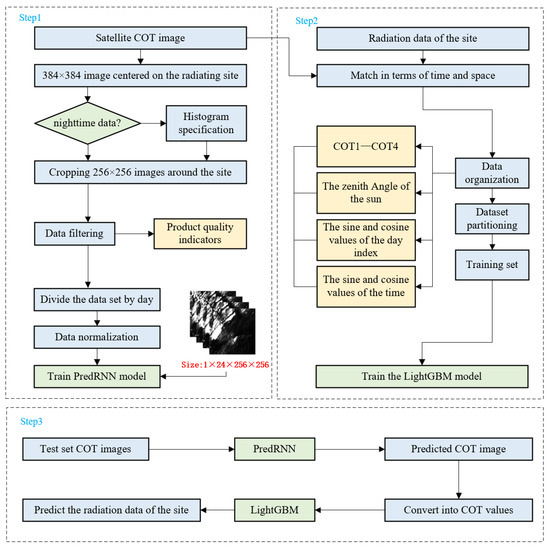
Figure 1.
Nowcasting the main process of surface solar irradiance at the site.
2.2.1. Cloud Optical Thickness Prediction Module
The PredRNN model [31] is an improved recurrent neural network (RNN) designed for spatiotemporal sequence prediction, utilizing a spatiotemporal memory flow to enable cross-layer information interaction while decoupling long-term and short-term dynamic modeling. Validation on existing datasets had demonstrated that PredRNN outperforms traditional models like ConvLSTM and Trajectory Gated Recurrent Unit (TrajGRU) in metrics such as Root Mean Square Error (RMSE), Structural Similarity Index (SSIM), and Learned Perceptual Image Patch Similarity (LPIPS) [31]. Therefore, we applied PredRNN model for future 3-h COT forecasting. We input 12 COT images with a 15-min interval and output 12 frames of future COT images. The data organization format was in shape [number of images, number of channels, 256, 256], and the network’s structure was set to four layers, each containing 128 neurons. At the same time, we optimized the training process and the loss function to better learn the characteristics of cloud variations, while also improving prediction accuracy.
- (1)
- Loss Function
In COT image prediction, the loss function was primarily used to describe the differences between the predicted sequence of 12 future images and the actual sequence of 12 future images, as well as the similarities between the incremental memory states of the two types in the model. During the training phase, after each batch of training data is fed into the model, a forward propagation process outputs the predicted COT images. Then, the loss function calculated the difference between the predicted values and the actual values, i.e., the loss value. Once the loss value was obtained, the model would update the weights through backpropagation to minimize the loss between the actual and predicted values, enabling the model’s predictions to gradually approach the actual results, thereby achieving the learning objective. The loss function , used in the initial training phase, was expressed as follows:
where represents the squared error between the predicted image sequence output by the model and the true image sequence. The inner notation represents the L2 norm (Euclidean norm), which calculates the “distance” between predicted and true values across dimensions. The outer squared notation is used to simplify computation and enhance the penalty for difference. represents the structural similarity error between the predicted image sequence and the true image sequence, and represents the memory decoupling loss, which is a regularization loss proposed in paper [31] aimed at the internal structure of the model, used to decouple spatiotemporal memory states and prevent redundant feature learning. represents the time step, represents the last output time step, is the predicted image at time , and is the true image at time . The mean SSIM is a metric used to measure the similarity between two images, comparing them in terms of luminance, contrast, and structure. The specific calculation formula is as follows:
where , and represent the luminance similarity, contrast similarity, and structural similarity, respectively, between the predicted image and true image. Typically, . Compared to using SE as a loss function, SSIM can more effectively help the model learn the nonlinear features of cloud motion [28], preserving the edges and structure of the clouds, thus improving the physical realism of the prediction. Meanwhile, retaining SE as part of the loss function guides the model to predict relatively accurate COT values, avoiding situations where the predicted image appears visually correct but the actual values differ significantly, thereby ensuring the accuracy of subsequent radiation predictions.
- (2)
- Center Enhancement
During the model training and prediction process, although the input image size was 256 × 256, the COT prediction results for the central site and its adjacent area were what we focused more on. However, in the early stages of model training, the loss function was computed over the entire 256 × 256-pixel area, without targeted learning for the central region. Therefore, after a certain number of training iterations, we introduced a center enhancement strategy by adjusting the computation of the loss function to focus on a 10 × 10-pixel area at the image center, while still using SE and SSIM to calculate the loss value over the entire image. We also attempted to train the model from scratch while restricting the loss computation to the small area centered on the station. This strategy, however, led the network to predict almost clear-sky conditions (COT ≈ 0) across the entire center. We conjecture that this behavior arises because the confined central region is prone to domination by either clear or cloudy scenes. When clear skies or thin clouds prevail, the model minimizes the global training loss by predicting uniformly low COT values within this region. Additionally, the limited spatial extent prevents the model from capturing large-scale cloud-motion dynamics, revealing a significant limitation of this localized approach. At this point, the loss function consisted of four parts: SE, SSIM, the Mean Squared Error (MSE) of center region between predicted and actual images, and the cosine similarity of long-term and short-term dynamic memory cells. The specific expression is as follows:
where the expressions for and are the same as those used in the early stages of training, i.e., they are identical to the three components in Equation (1). In Equation (6), represents the predicted image for the 10 × 10-pixel region at the image center, and prime represents the true image for the 10 × 10-pixel region at the image center. Finally, the model outputs the COT prediction images for the next 3 h at 15-min intervals. The COT mean values for the center pixel and its surrounding regions were extracted and organized to estimate the future 1-h, 2-h, and 3-h radiation results for each test case, which were then compared with satellite observations for validation.
- (3)
- Result Evaluation
The evaluation metrics consisted of statistical indicators for the prediction of COT values and classification accuracy metrics for cloud classification based on the COT prediction results. In the evaluation of COT prediction results, we compared the predicted future frame sequences with the corresponding true frame sequences at each time step. The MSE, RMSE, SSIM, Mean Bias Error (MBE), Mean Absolute Error (MAE) between the predicted and actual COT images from the test set and Forecast Skill (FS) metrics were used for evaluation, and the corresponding calculation formula is as follows:
where represents the case number in the test set, represents the total number of test cases, denotes the time step of the predicted frame, is the time step of the last known input image in the sequence, represents the first frame of the predicted future sequence, and represents the last frame of the predicted future sequence. represents the predicted frame image, and represents the corresponding actual image. The smaller the MSE, RMSE and MAE values are, the closer the MBE is to 0, and the closer the forecast result is to the true result. In Equation (11), and represent the RMSE value of the evaluated model and reference model, respectively. If FS is greater than 0, it indicates that the forecast performance of this model is better than that of the reference model at this moment. The larger the FS value, the more the forecast performance is better than that of the reference model, indicating a more accurate forecast. For the convenience of calculation, we take the regular persistence in the performance evaluation of COT image prediction as the reference model, taking the last observation (i.e., ) as the prediction result for the next 12 frames.
In addition, we classified clouds based on COT values to evaluate the accuracy of the forecast results for cloud type prediction. The classification criteria were based on the method proposed by the International Satellite Cloud Climatology Project (ISCCP) [34] and are described as follows:
To evaluate the accuracy and the trend of cloud type prediction for the next 12 time steps, we used the following metrics: confusion matrix at each time step, accuracy, and kappa coefficient. The definitions of these metrics are as follows:
where represents the total number of pixels involved in the classification, denotes the true class label at the i-th pixel, and denotes the predicted class label. In Equation (14), represents the observed consistency, i.e., the proportion of times the predicted label matches the actual label, and represents the expected consistency, i.e., the probability of a random prediction matching the actual label. The values of accuracy and kappa coefficient indicate the quality of the classification. Specifically, accuracy represents the proportion of correctly classified samples out of the total samples, while the kappa coefficient measures the precision of the classification. In Equation (15), is the value at the position of row i and column j of the confusion matrix, and is the corresponding value in the normalized confusion matrix. refers to the number of pixels where the classifier correctly predicts a positive sample, and the actual value is also positive. refers to the number of pixels where the classifier incorrectly predicts a negative sample, but the actual value is positive. The normalization of the confusion matrix using the specified formula was designed to enable a unified comparison of prediction accuracy across different cloud types, with a focus on the distinct physical characteristics of cloud–radiation interactions. In solar radiation prediction, the transition from cloud-free to thin-cloud conditions can result in a significant increase in surface shortwave radiation flux. In contrast, the progression from thin-cloud to thick-cloud conditions leads to an exponential decrease in radiation impacts. Given that the absence of accurate thin-cloud detections can substantially increase radiometric prediction errors, the accurate identification of thin-cloud conditions is of paramount importance. In this study, the confusion matrix was row-normalized using Recall to emphasize the accuracy of thin-cloud detection.
2.2.2. Surface Solar Irradiance Prediction Module
LightGBM is a boosting framework proposed by Microsoft Research Asia (MSRA) [35], which performs excellently in handling large-scale data and high-dimensional features, with advantages such as fast training speed, low memory consumption, and flexible usage [36,37,38]. In this study, we employed the LightGBM model to predict the SSI at the station, with the following input features: day of the year, time of day, solar zenith angle, the sine and cosine values of the day of the year, the sine and cosine values of the time of day, average COT values for different-sized regions above the ABQ station (the pixel regions of interest included the central pixel (COT1) and surrounding areas of 2 × 2 (COT2), 4 × 4 (COT3), and 6 × 6 (COT4) pixels.). The multi-scale COT parameterization was designed to consider the differential modulation mechanisms of cloud layers on solar radiation transmission. The COT1, defined as the vertical-path integrated COT over a localized area above the measurement site, characterized the vertical attenuation of direct shortwave radiation by cloud layers. An increase in COT1 induced an exponential reduction in ground-level direct radiation flux. In contrast, the regional mean COT parameters (COT2-4), derived through spatial averaging algorithms, resolved the influence of cloud horizontal heterogeneity on three-dimensional scattering processes that occur inside clouds or between neighboring clouds. Under thin-cloud conditions, enhanced intra-cloud multiple scattering elevates the total surface radiation, whereas when COT exceeds the critical threshold, the cloud-top albedo-driven radiative reflection mechanism dominates, significantly reducing the net surface radiation. This multi-scale parameterization framework provided theoretical support for accurate solar radiation prediction by independently constraining vertical attenuation and horizontal scattering processes in radiative transfer modeling. Furthermore, the solar zenith angle (sza), which influences the radiation received at the ground station, was also used as an input parameter. To capture the periodic characteristics of solar radiation changes with respect to the date and time, we converted the day of the year (jday) and the time of day (dt) into angles and calculated their corresponding sine and cosine values (sin_jday, cos_jday, sin_dt, cos_dt) to better capture their periodic features.
During the prediction phase, the predicted COT values (COT1 to COT4) were combined with the previously defined parameters as model inputs. The trained LightGBM model subsequently output SSI predictions for each target time point. For evaluating the SSI estimation results, we used the Pearson correlation coefficient (R), MSE, RMSE, MBE, MAE between the predicted and actual SSI values from the test set and FS as the evaluation metric. The closer the R is to 1, the better the estimation performance. The calculation formula of R is as follows, and others can refer to Equations (7)–(11):
where and represent the predicted radiation value and the actual radiation value of the i-th sample, respectively, and are the mean values of all predicted and actual radiation values, and is the number of samples.
Specifically, in Equations (7)–(11), the difference in meaning of the formula parameters in the COT forecast is that n represents the number of test samples, not the number of pixels. Here, in Equation (11), we select the convex combination of the regular persistence (PERS) with the climatological as reference [39,40,41], which means that the reference model is constructed through the optimal convex combination of regular persistence and climatological values, integrating short-term observational patterns (current irradiance state) and long-term statistical patterns (the historical average state at this moment over three years). The average SSI for each moment was calculated using the SSI measurement data from the ABQ site from 2020 to 2022, and the short-term observational patterns were SSI values estimated by LightGBM from the last observed COT in corresponding cases (the specific calculation process is detailed in Appendix B.1).
3. Results
In Section 3.1 and Section 3.2, we independently verified the COT image prediction model and the SSI estimation model. Then, in Section 3.3, we connected the above two models to assess the performance of irradiance nowcasting. Finally, in Section 3.4, we analyzed the characteristics of the newly proposed algorithm through case studies.
3.1. Cloud Prediction
3.1.1. COT Forecast
In this study, we developed three different models (M1, M2, and M3) for predicting COT images to evaluate the effects of training with the nighttime data and employing the center enhancement strategy. M1 represents a model trained using the nighttime data along with the center enhancement strategy. M2 retains the nighttime data but excludes the center enhancement strategy. M3 further removes the nighttime data and also does not utilize the center enhancement strategy. The performance of these three models is evaluated within a 10 × 10-pixel region of interest surrounding the target site.
Figure 2 shows the significant superiority of M1 and M2 models, which were trained with the nighttime data, achieving a maximum MSE improvement of ~125 at T + 8 compared to M3. Before T + 2, all three models exhibit comparable predictive performance. However, after T + 2, the divergence in MSE between M1, M2 and M3 progressively increases. By T + 11, the mean improvement of M1 over M3 reaches 15–53% (with the minimum improvement occurring at time step T + 10, where the MSE decreases from 287.939 to 245.15, and the maximum improvement occurring at time step T + 8, where the MSE decreases from 246.158 to 123.863), underscoring the critical role of incorporating nocturnal data into the training process to enhance the precision of COT prediction within the image. Furthermore, from T + 1 to T + 10, the performance of M1 and M2 remains comparable, albeit with M1 holding a slight edge. Notably, after T + 10, the MSE of M1’s forecasts drops significantly, which attests to the fact that employing a central reinforcement strategy can substantially augment the accuracy of COT prediction in the central image region.
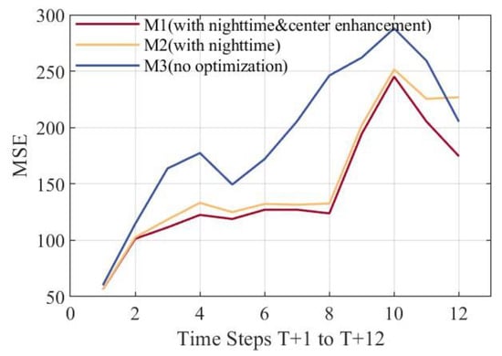
Figure 2.
The effects of training with the nighttime data and employing the center enhancement strategy. The x-axis represents prediction time (T + 1, T + 2……T + 12) with a time step of 15 min by the cases, and the y-axis represents the average MSE between the predicted images and the actual images at the corresponding moments of all test set cases.
The trend of MSE over time for M2 and M3 shows that in the 10 × 10-pixel region of interest prediction, MSE remains stable until T + 8, maintaining between 100 and 150 from T + 2 to T + 8, then rises rapidly to a peak of 250 at T + 10, and shows a significant downward trend after T + 10. The instability observed in the local region forecasts, compared to the full-image forecasts, can be attributed to several factors. Firstly, local errors are more likely to be amplified and highlighted compared to those in a larger full-image area. The smaller number of pixels in the local region cannot effectively average or dilute the larger errors within the area, especially when the central small region happens to be where the cloud changes are more complex. Secondly, the scope of the loss function during model training is still primarily based on the full image. Even when using a center enhancement strategy, the model does not discard the statistical calculation of the loss function for the entire image. This results in the model having limited and unstable prediction capabilities for small-scale and fine structures. As shown in Appendix A Figure A2, in contrast, the MSE curve of larger image regions (256 × 256-pixel regions) exhibits a more stable trend over time. This is because larger image regions can provide richer contextual information, helping the model better comprehend and predict the evolution trends of images, thus enhancing prediction stability. This underscores the importance of optimizing the spatial range selection of the images, allowing the model to learn from a broader spatial range of COT product images.
Additionally, to more intuitively demonstrate the effectiveness of incorporating nighttime data into the training dataset, we present the prediction results from M2 and M3 in Figure 3a,c respectively present the forecast results of the night and daytime cases. Corresponding time series comparison graphs of the SSIM and its component indices for both models were plotted in Figure 3b,d to further verify the advantage.
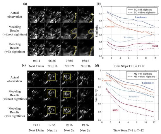
Figure 3.
Nighttime and daytime cloud-motion cases. (a) and (c) show the evolution of COT in each case, which represent nighttime and daytime cases, respectively. The time is labeled in UTC. From left to right are the prediction results for the next 15 min, 1 h, 2 h, and 3 h. Yellow lines outline the main cloud-mass morphology. And yellow boxes outline the areas that need attention in the daytime case. (b) and (d) present the performance of SSIM and its components at different times for nighttime and daytime cases, respectively. The x-axis shows future time steps (T + 1 to T + 12), and the y-axis shows the values of SSIM and its components. The closer to 1, the higher the similarity of prediction and actual observation. Dark blue, orange, light blue, and red curves represent luminance similarity, contrast similarity, structural similarity, and SSIM, respectively. Solid lines are for M2, and dashed lines for M3.
In Figure 3a, it is evident that M2 has an advantage in capturing structural features, with the forecast of cloud shapes on the right side of the image being closer to the real situation. In Figure 3b, in terms of luminance similarity, both models initiate with values close to 1, indicating high initial similarity. However, this similarity declines over time for both models. Notably, M2 consistently outperforms M3 in maintaining higher luminance similarity. This superior performance is advantageous for enhancing the accuracy of COT predictions, thereby improving the overall prediction outcomes. Regarding contrast similarity, models M2 and M3 exhibit a decline over time. In contrast, structural similarity remains relatively stable across the forecast period. Before T + 4, structural similarity decreases, likely due to the model’s initial difficulty in adapting to the structural features of the data. However, after T + 4, structural similarity increases as the model becomes better adapted. Throughout the forecast period, M2 consistently outperforms M3 in structural similarity. The abovementioned outcomes demonstrate the important role of nighttime data in enhancing the stability and accuracy of long-term predictions by image generation or prediction models.
As shown in Figure 3c, the two models had similar prediction results at the 15-min forecast, with high similarity to the actual images. However, as the forecast time increased to 1 h, 2 h, and 3 h, significant differences emerged between the forecast images. Notably, in the forecast images for 1 h and 2 h, focusing on the yellow-framed area, we found that M2 could better predict the shape and location of cloud holes, which is crucial for accurately forecasting radiation at corresponding positions. Figure 3d reveals that the SSIM components and overall SSIM metrics were almost identical at the 15-min forecast. As the time steps increased, all metrics declined, but M2 consistently outperformed M3 at each time step. Combining these findings with nighttime cases, it is evident that incorporating nighttime data not only enhances the accuracy of nighttime COT predictions but also improves the prediction performance for daytime cases. This improvement is likely due to the enriched dataset from the inclusion of nighttime data, which allows the model to learn more diverse cloud movement and change patterns under various conditions, thereby enhancing its generalizability and resulting in better performance across different cases.
3.1.2. Cloud Classification
Figure 4a,b show the curves of the overall accuracy and kappa coefficient of cloud classification prediction varying with the increase in forecast time, respectively. Figure 4a shows that the model maintains a high classification accuracy with an average value exceeding 0.8, reaching around 0.9 at T + 1. However, Figure 4b shows that the performance of the kappa coefficient is relatively weaker, with the highest value appearing at T + 1, slightly above 0.6, and dropping to around 0.25 at T + 12. Despite the high classification accuracy, the low kappa coefficient reflects a severe imbalance in the sample proportions of different categories in the dataset, with the model tending to predict all cloud pixels as the most frequent category.
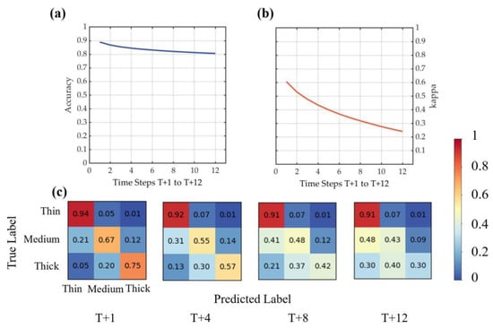
Figure 4.
Cloud classification results for the next 12 steps of the full 256 × 256 image. The x-axis of each curve diagram represents future time steps (T + 1 to T + 12), with a 15-min time step. The y-axes of (a) and (b) indicate the evaluation values of classification accuracy and the kappa coefficient, respectively. (c) presents the normalized confusion matrices for the next 15 min, 1 h, 2 h, and 3 h.
Figure 4c plots the normalized 3 × 3 confusion matrix for the future timesteps. Each row represents the true class, while each column represents the class predicted by the model, including thin, medium-thick, and thick clouds. The elements on the diagonal of the matrix indicate the proportion of samples correctly predicted by the model for each true class, and vice versa for the proportion of samples incorrectly predicted by the model. It can be observed that, in the first time steps, the model exhibits no significant bias in cloud type forecasting, especially as the thin cloud reaches a very high accuracy of 0.94. As time passes, the model’s prediction gradually deviates, with the accuracy of medium-thick clouds decreasing from 0.67 to 0.43, and the prediction accuracy of thick clouds decreasing from 0.75 to 0.3, whereas the prediction accuracy of the thin cloud is relatively stable. A gradual increase in the values below the main diagonal in the confusion matrix indicates that the model tends to predict the cloud as thin or medium-thick. In other words, the model tends to underestimate the COT values. This phenomenon may be related to the climatic characteristics of the study area and the distribution of training data. Since the region where the station is located has a mild and dry climate, thin clouds occupy a large proportion of the training dataset, and the model may have developed a stronger bias toward predicting thin clouds while performing relatively poorly on medium-thick and thick clouds. Nevertheless, since our primary focus in radiation forecasting is the impact of the transition from clear skies to cloudy conditions on radiation, the model’s precise forecasting of thin clouds effectively captures this critical transition, thereby enhancing the accuracy of surface solar radiation predictions.
3.2. Irradiance Estimation
We validated the trained LightGBM model using the test set of the model. Figure 5a is the scatter plot of the estimated radiation values based on satellite-observed COT versus the true values, which shows that most points are clustered around the line y = x, with no significant overestimation or underestimation. Moreover, the overall correlation R between the two is 0.95656, demonstrating that the model has high estimation accuracy. Figure 5b illustrates the curves of the estimated radiation values and the actual radiation values for all cases in the test set, which shows that the trend of the predicted values closely follows that of the true values, demonstrating a high degree of alignment. These results provide strong evidence of the model’s effectiveness in the radiation estimation task. Additionally, the results of the LightGBM model for SSI estimation show that the correlation coefficients between the estimated and actual radiation values are 0.99 for clear skies and 0.93 for cloudy weather, with RMSE values of 26.48 and 97.43, respectively. This indicates that the model performs better under clear-sky conditions, where the correlation coefficient is close to 1 and the RMSE is much less than that under cloudy conditions. This difference in performance can be attributed to the fact that under clear skies, SSI is mainly influenced by the solar zenith angle and diurnal variations, resulting in a distinct parabolic shape of the radiation curve, which is easier to predict. In contrast, under cloudy conditions, the complex and variable nature of clouds significantly impacts radiation, increasing the difficulty of forecasting. However, by incorporating multi-scale COT parameters, our model still achieves a correlation coefficient of 0.93 for SSI estimation under cloudy conditions, which exceeds 0.9 and indicates relatively good performance.
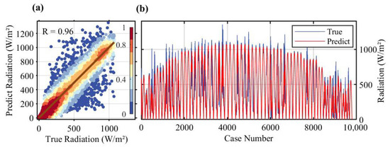
Figure 5.
Performance of the LightGBM model on the test set. (a) The x- and y-axes represent radiation observations and estimations (unit: W/m2), respectively, and the point color indicates the density of the scatter distribution; (b) The x-axis shows case numbers, and the y-axis shows radiation values, with red and blue curves representing predicted and true values, respectively.
To further validate the robustness of the model under different weather conditions, we selected two representative cases for analysis, with the results shown in Figure 6. The first case corresponds to clear weather (Figure 6a), where the model’s radiation estimation results nearly perfectly match the true values, with the R approaching 1 and the RMSE being minimal. This is likely because, under clear conditions, the primary factor influencing radiation estimation is the solar zenith angle, which is known and exhibits periodic variation over time, allowing the model to make high-precision estimations.
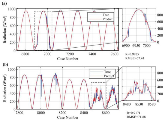
Figure 6.
Radiation estimation performance under clear/cloudy weather conditions. Large windows in Figure (a) and Figure (b) represent cases of a few days in the test sequence, while small windows illustrates the curves of radiation estimates and true values for a specific day under clear weather conditions and a specific day under cloudy weather conditions, respectively.
The second case corresponds to cloudy weather (Figure 6b), where frequent cloud cover changes over the station lead to deviations from the standard parabolic pattern of radiation. Despite this, the model still captures the radiation trend well, and the predicted values remain highly consistent with the true values, with a correlation coefficient of 0.92, and the RMSE between the SSI estimation results based on satellite-observed COT for all moments (with a 5-min interval) on the daytime of October 24th (case 2) and the actual site-observed SSI, which was 71.88 W/m2, while the radiation peak on that day was 610 W/m2. In comparison, the first case shows better estimation performance than the second. This is likely due to the increased difficulty in predicting COT images when cloud conditions are highly variable, resulting in larger estimation errors than in clear-sky conditions. And in this situation, the two factors that have the most significant impact on solar radiation estimation are the solar zenith angle and the COT values around the station. Inaccurate predictions of COT values in the previous step may further affect the accuracy of solar radiation estimation. Overall, the model demonstrates good performance under different weather conditions, achieving excellent prediction results on the overall test set. The results of the case study further confirm the stability and reliability of the model.
3.3. Irradiance Nowcasting
By combining the cloud forecast model and the irradiance estimation model, we can achieve irradiance nowcasting. The performance of this irradiance nowcasting method was validated using observation data from the ABQ station. To conduct our test, we selected cases of 2 days every 10 days over one year, ensuring that these cases did not overlap with the training data in terms of time. For each case, we predicted the COT images for the future after 1 h, 2 h, and 3 h. The predicted COT images were converted into the average COT values of four regions, such as 1 × 1 (COT1), 2 × 2 (COT2), 4 × 4 (COT3) and 6 × 6 (COT4) -pixel areas around the ABQ station, to characterize the ability of clouds to influence direct and scattered radiation.
Table 1 is used to evaluate the COT prediction accuracy of our model under different circumstances, which shows the correlation coefficient between the predicted and the true COTs of our model for three cases, assuming that nighttime data were included when training. The “Alltime” involves all cases in the test set, “Daytime” and “Transmissivity” for all daytime cases. In the expression for the transmissivity, COT represents the exponential rate at which the radiation is extinguished within an absorbing or scattering medium. Among the four COTs, COT4 always has the best correlation coefficient, since calculating an average over a larger area reduces the requirement for the accuracy of the model’s prediction of cloud movement. We trained the cloud forecast model on the entire dataset. However, across all COT averages, the model demonstrated improved performance on the daytime test set compared to the all-time test set, with gains of approximately 0.03 (next 1 h), 0.11 (next 2 h), and 0.16 (next 3 h), respectively. This enhancement is attributed to the relatively poorer quality of nighttime data, which compromised model evaluation on the full dataset.

Table 1.
Correlation coefficients between the predicted and the true COTs.
As shown in Table 1, in terms of daytime test, the COT predictions show less-than-ideal correlation coefficients, particularly for COT1. For the future 3-h predictions, the correlation coefficients of COT1 do not exceed 0.5, and decrease as the time step increases, ultimately reaching the lowest value of 0.38. This relatively low correlation coefficient indicates that it is difficult to make accurate COT predictions at specific points (single pixel). The uncertainty of the COT measured by satellites is also a factor contributing to the low correlation coefficient. Similarly, the correlation coefficient of COT4 shows a decreasing trend as the forecast duration increases. It reaches its lowest point of 0.62 in the 3 h of the future. Nevertheless, this is still much more accurate than COT1 at each moment. As indicated by the input variable importance ranking in LightGBM (provided in Appendix A Figure A3), COT4 is the primary influencing factor for irradiance estimation. Consequently, this reduces the impact of biased COT1 on the irradiance nowcasting.
Rather than focusing on the accuracy of the COT prediction, we are more concerned with its ability to predict the changes in atmospheric radiative transfer related to the COT. This is the key factor that affects the surface solar irradiance. The Beer–Lambert law indicates that the effect of COT on solar radiation attenuation follows an exponential decay relationship in terms of transmissivity, i.e., (where is the COT value) [42]. We calculated the correlation coefficient between the transmissivities (i.e., and ). As shown in Table 1, applying the exponential operation significantly increased these correlation coefficients due to the saturation effect. Specifically, the first row of each timestep in Table 1 shows the correlation coefficients before the exponential operation, while the third row shows the correlation coefficients after the exponential operation. For relatively large COT values, even inaccurate predictions can yield similar transmissivity, reducing the impact on solar irradiance forecasts. For example, the correlation coefficients for COT1 over the next 1 h, 2 h, and 3 h increase to 0.73, 0.64, and 0.58, respectively. The correlation coefficients for COT4 increase to 0.80, 0.71, and 0.65, laying a solid foundation for the subsequent accurate prediction of SSI.
Finally, we used the above COT prediction results to forecast the SSI. Figure 7 presents the scatter plots and line charts of the predicted and actual radiation curves for the future after 1 h, 2 h, and 3 h. It can be seen that the radiation predictions exhibit a high degree of correlation with the actual values, with correlation coefficients of 0.94, 0.92 and 0.92, which improves 7.3%, 4.5% and 4.2% compared with the assessment results that do not take COT into account but only consider cyclical changes. As illustrated in Box 1 (for clearer images in the box, refer to the Appendix A Figure A5), under favorable weather conditions (with almost no clouds in the study area), the radiation forecast and the actual results match closely, and the forecast is less influenced by the COT prediction results. However, when radiation values are very high, as shown in Box 3, there is an underestimation of the prediction. Moreover, there are discernible differences in the predictions for the future after 1 h, 2 h, and 3 h. Specifically, the prediction curve for the future after 1 h demonstrates the closest fit to observations, while 2-h and 3-h predictions maintain alignment generally, though they omit finer details. For example, the subtle radiation dip in Box 2 is captured at future 1 h and 2 h but missed at future 3 h, reflecting the inherent decrease in prediction accuracy with extended forecast times. Overall, predicted trends consistently match reality, providing actionable forecasts for photovoltaic plant operations.
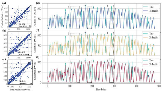
Figure 7.
Scatterplot of true vs. predicted future 1-h, 2-h, and 3-h radiation values and surface solar irradiance forecasting results for all daytime cases. Figures (a–c) represent the scatter plots of the predicted and actual radiation values for the next 1 h, 2 h, and 3 h, respectively. Figures (d–f) show the line charts of the predicted and actual radiation curves for the corresponding time steps.
3.4. Case Studies
After presenting the complete radiation prediction results for the test set, we further analyze the model’s performance on different types of cases by focusing on a few representative ones. Based on characteristics such as cloud movement speed, observation time, and cloud distribution shape, we selected the following two representative cases for analysis. Figure 8a,c display the COT images of the cloud-motion sequences for case 1 and 2, respectively. Figure 8b,d present the comparison curves of the predicted and observed radiation values at 15-min intervals for the next three hours.
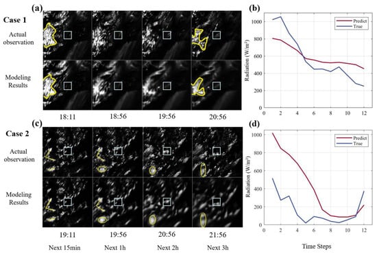
Figure 8.
Representative cloud-motion cases. The first column shows the evolution of cloud optical thickness in each case, labeled in UTC. Yellow contours outline the main cloud-mass morphology. The second column presents radiation prediction results. The x-axis indicates future time steps (T + 1 to T + 12), and the y-axis shows radiation values (unit: W/m2). Red and blue curves denote predicted and true values, respectively. Figures (a) and (c) display the COT images of the cloud-motion sequences for case 1 and 2, respectively. Figures (b,d) present the comparison curves of the predicted and observed radiation values at 15-min intervals for the next three hours.
3.4.1. Case 1: Cloud Moves Fast
A case with significant cloud cover changes within a three-hour period was selected for in-depth analysis. The movement of the yellow cloud mass highlighted in Figure 8a demonstrates the model’s ability to effectively capture the movement and morphological changes of the main cloud masses from 15 min into the future up to the 3-h time period. The light blue box in the center of the COT image (central region) transitions from clear sky to thin clouds in line with the trend in Figure 8b, where radiation decreases with increasing time. This trend can be attributed to the case occurring in the afternoon when solar radiation naturally decreases, and the presence of clouds in the central region further attenuates the radiation reaching the ground. Consequently, the radiation continues to decrease, and the forecast values are consistent with the actual values in this regard. It is worth noting that the slight increase in the actual radiation value before T + 2 in Figure 8b is due to the period being before noon when solar radiation increases. Our model may not have captured this accurately because it is more adept at identifying patterns and trends in radiation changes but has certain limitations in forecasting extreme values. The numerical observation shows that the forecast radiation value is close to the actual radiation value, which to some extent reflects the advantage of the first-step COT forecasting model in predicting thin clouds.
3.4.2. Case 2: Scattered Small Clouds
As depicted in the case sequence diagram (Figure 8c), the model demonstrates robust performance in forecasting scattered cloud distributions. In Figure 8d, the radiation reaches a trough at around T + 8 and gradually increases with time, which is consistent with the cloud motion depicted in the boxed area of Figure 8c. Prior to UTC 20:56 (T + 8), the light blue boxed area is predominantly characterized by clear skies and thin clouds. The variation in radiation is primarily influenced by the solar zenith angle and is also affected by the movement of clouds. By UTC 20:56, a thick cloud appears in the center of the box, significantly attenuating solar radiation and causing a substantial drop in the radiation value. At 21:56, it can be observed from the corresponding boxed area in the COT image at that time that the cloud which blocked the station center at T + 8 has moved away. Consequently, the radiation value reverts to a state predominantly modulated by the solar zenith angle, thus exhibiting an upward trajectory. Thus, the forecasts capture the above trends well, but numerically the forecast values are higher than the actual radiation values, probably due to the underestimation of COT in the initial model.
4. Discussion
To further substantiate the advantages of our proposed framework in COT prediction and SSI nowcasting while simultaneously delineating its limitations, this Section presents a further comparative analysis.
4.1. Comparative Assessment of Irradiance Nowcasting Methods
This Section is organized into two parallel comparisons: COT prediction across different approaches and the solar irradiance forecast performance derived from each COT product.
To better demonstrate the COT forecasting performance of various state-of-the-art models [43], we evaluate the forecasted COT images against the true COT images at corresponding time steps using several metrics: RMSE, SSIM, MAE, MBE, and FS. The models compared include optical flow methods [44], ConvLSTM [28,45], PredRNN [31] and our model, which are based on satellite observations. Specifically, the optical flow baseline follows Farneback’s dense-flow algorithm [46]. ConvLSTM shares the same input/output tensors, network depth and neuron count with our PredRNN but replaces the spatiotemporal memory cell with the standard ConvLSTM cell. ConvLSTM implicitly captures spatial features by replacing fully connected layers with convolutional layers, which focus on time series processing and are computationally simpler. PredRNN builds upon this by introducing a spatiotemporal gating mechanism, explicitly separating spatial and temporal states to enhance the modeling capability for complex spatiotemporal dynamics. This enhancement, however, comes with higher computational complexity. And “PredRNN” in the pictures and clarifications on comparison of different models denotes the baseline model without the revised loss function or the center enhancement strategy introduced in our study. All models were evaluated on the complete ABQ test set for horizons up to 3 h ahead.
As shown in Figure 9, our model has a slight advantage over other models in terms of overall image performance. (a) and (e) show that curves of PredRNN and our model almost overlap in two metrics, indicating that our model has similar performance to PredRNN in RMSE and FS. Additionally, in RMSE, our model is superior to ConvLSTM before T + 4 but similar thereafter and consistently outperforms the optical flow method at all forecast times. Notably, (b) shows that the bias of our model increases from zero to negative values, indicating a systematic underestimation of COT while other comparison models have MBE values fluctuating between −0.5 and 0.5. (c) reveals that our model has the lowest MAE among all models at each time step, suggesting that while our model’s forecasts have smaller deviations overall, they tend to be negatively biased. Moreover, our model’s superior SSIM performance is attributed to the inclusion of the SSIM index in the loss function during training, enabling the model to better capture changes in the structure, brightness, and contrast of COT images, which can further improve the irradiance estimation.
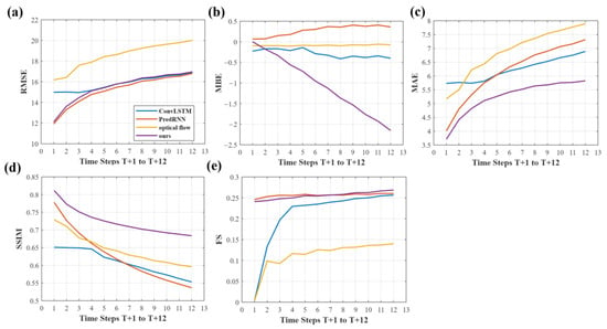
Figure 9.
The performance of four different models in COT image prediction. The x-axis represents prediction time (T + 1, T + 2……T + 12) with a time step of 15 min, and the y-axis represents the model’s performance in relevant metrics. The value at each time step represents the average of the errors between the predicted values and the true values or forecasting skill at the corresponding moments of all test set cases. Figures (a–e) respectively show the performance of different models in terms of RMSE, MBE, MAE, SSIM, and FS indicators. The blue, orange, yellow, and purple curves represent the ConvLSTM, PredRNN, optical flow, and our model, respectively.
Beyond overall image performance, our model excels in predicting COT in smaller regions around stations, which is crucial for subsequent SSI forecasts. Figure 10a shows that in terms of RMSE for 10 × 10 local COT forecasts, our model performs similarly to PredRNN before T + 3 but surpasses it by 1.9% (T + 4) to 11% (T + 12) afterwards. (b) and (c) reflect a similar underestimation phenomenon as seen in the full-image forecasts. (d) indicates that our model also has the highest SSIM values for local region forecasts, not only on the overall image. (e) shows that our model’s FS values are consistently above 0 and close to 0.5, significantly higher than those of other models, with a range of 0.1 (T + 1) to 0.51 (T + 12) higher than the second-best PredRNN. This advantage is likely due to the central enhancement strategy we employed, which improves the model’s ability to capture COT changes in the central region of the image. This improvement is highly significant for enhancing the accuracy of subsequent SSI forecasts.
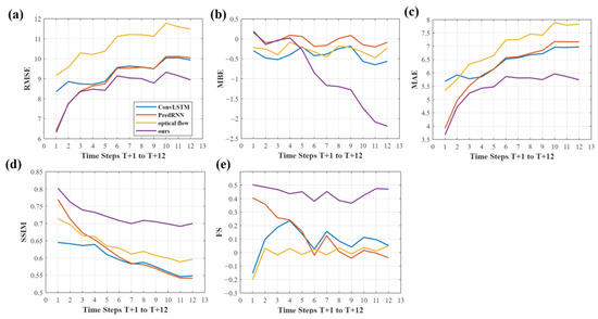
Figure 10.
The performance of four different models in COT image prediction of local region. The x-axis represents prediction time (T + 1, T + 2……T + 12) with a time step of 15 min, and the y-axis represents the model’s performance in relevant metrics. The value at each time step represents the average of the errors between the predicted values and the true values or forecasting skill at the corresponding moments of all test set cases. Figures (a–e) respectively show the performance of different models in terms of RMSE, MBE, MAE, SSIM, and FS indicators. The blue, orange, yellow, and purple curves represent the ConvLSTM, PredRNN, optical flow, and our model, respectively.
To further and more comprehensively evaluate the advantages of our model, we have examined multiple models in R, MSE, RMSE, MBE, MAE between the predicted and actual SSI values from the test set and FS of different models. Relative formulas have been showed in Section 2.2.2, Equations (7)–(11) and (16).
During the SSI nowcasting process, in addition to using the three comparison models of COT forecast, we also added another model, Long Short Time Memory (LSTM) [47]. The LSTM baseline still operates on COT: the regional satellite-observed COT centroid COT1 and the area-averaged values for COT2–COT4 are concatenated into a 12-step (3 h) time series, respectively, which is then used to predict the next 12 COT values; these predicted COTs are finally fed into a LightGBM regressor to obtain the SSI forecast. All models were evaluated on the complete ABQ test set for horizons up to 3 h ahead.
In Table 2, the first column, Timesteps, represents the predicted future moment, with each moment corresponding to the five different models in the second column, model. The remaining columns respectively contain six evaluation indicators.

Table 2.
The performance of the model in various indicators.
As shown in Table 2, our method outperforms all competing models on almost every metric. For the 3-h horizon, RMSE improves by 7.7%, 1.8% and 12.6% relative to the second-best PredRNN at 1 h, 2 h and 3 h, respectively. The MBE values (in W/m2) compared with most baselines drop below 10, and are close to 0 in our model, indicating a substantial reduction in systematic error. Moreover, our forecasts remain stable across the full 3-h window: the FS score decreases only modestly from 0.71 to 0.66 and stays above 0.65, whereas the PredRNN drops from 0.66 at 2 h to 0.61 at 3 h, revealing a marked performance decline in the last two hours.
Our model’s superior performance is due to several key enhancements. Firstly, unlike LSTM, which only considers temporal variations of COT, our model captures spatially integrated changes across a broader area, improving COT mean value predictions for central stations and their vicinity, and enhancing overall forecast precision. Secondly, compared to optical flow methods, our model better captures the nonlinear dynamics and complex life cycle of clouds, leading to more accurate SSI forecasts. Thirdly, our model incorporates a spatiotemporal memory cell, overcoming ConvLSTM’s limitations by propagating memory information across both dimensions, boosting COT forecasting performance. Lastly, our refined loss function and central enhancement strategy improve COT prediction accuracy and SSI nowcasting, further validating our approach’s effectiveness.
4.2. Irradiance Nowcasting Performance Across Diverse Sites
The preceding validation at ABQ already demonstrated the feasibility of translating satellite-derived COT forecasts into SSI predictions. To test whether this success can be replicated under contrasting climates and synoptic regimes, we replicated the full workflow at two geographically and meteorologically diverse stations: Madison, Wisconsin (MSN; 43.13°N, 89.33°W) and Salt Lake City (SLC; 40.77°N, 111.97°W). Each site followed the same time range and experimental protocol, including spatially cropping COT images over the station domain, constructing training and test sets, training the improved PredRNN model, and feeding the resulting three-hour COT forecasts into LightGBM to predict SSI. The forecast performance is reported in Table 3.

Table 3.
The performance of irradiance nowcasting in different sites.
Table 3 shows that, apart from the excellent performance at ABQ, the model also performs well at SLC: the correlation coefficients between the 3-h forecasts and observations exceed 0.9 and the RMSEs remain below 150 W/m2. Additionally, the skill at MSN remains solid, with correlations comfortably above 0.8 and RMSEs near 160 W/m2, only slightly inferior to those at the best-performing sites. This modest shortfall is likely attributable to the site’s low-lying, humid environment, which introduces additional microphysical complexity not fully captured by the current predictors. The results show that, despite site-dependent variations linked to geography, SSI forecasts remain consistently accurate, attesting to the framework’s broad applicability across diverse locations.
5. Conclusions
This study innovatively replaces conventional satellite cloud imagery inputs with COT product images to better characterize solar radiation attenuation for site-specific irradiance prediction. The PredRNN model was employed for COT forecasting, incorporating several key enhancements during prediction: optimization of input image spatial range, improvement of the loss function, implementation of a center enhancement strategy, and augmentation of training diversity through nighttime data integration. Collectively, these improvements strengthened the model’s capacity to interpret diverse atmospheric conditions and enhanced prediction accuracy for both target sites and adjacent regions. Empirical validation confirmed an average 25.8% reduction in MSE for 15-min-interval global COT predictions over 3 h compared to baseline performance (the M1 model without any optimization). The transmittance derived from COT4 (the 6 × 6-pixel regions of interest, critical for radiation modeling) is closely correlated with the observed values of 0.80 (1 h), 0.71 (2 h), and 0.65 (3 h), enabling high-accuracy solar radiation prediction. Based on these COT predictions, a LightGBM model integrated multi-scale regional COT averages for the ABQ site to estimate its solar radiation. The model achieved remarkably high correlations between predicted and observed irradiance: 0.94 (1 h), 0.92 (2 h), and 0.92 (3 h). By enabling high-accuracy ultra-short-term surface solar irradiance forecasting, this framework provides critical support for planning distributed PV stations within satellite-observable areas.
Although this study has achieved some noteworthy results, there are still several areas worthy of further exploration and improvement. Specifically, it is important to enhance the model’s generalization capability so that it can accurately predict COT for clouds of various thicknesses. Also, incorporating multi-source meteorological data (e.g., wind speed, temperature) into the COT prediction model may further boost COT forecasting accuracy. Furthermore, transforming the current two-step model into an end-to-end model would make it possible to predict radiation directly, thereby reducing error propagation from separate models.
Author Contributions
Conceptualization, Y.Y., J.Y. and S.L.; methodology, J.Y., Y.Y. and S.L.; validation, Y.Y., J.Y. and J.D.; formal analysis, Y.Y. and Z.L.; investigation, Y.Y., T.L. and Z.Z.; resources, J.Y. and S.L.; data curation, Y.Y. and J.Y.; writing—original draft preparation, Y.Y.; writing—review and editing, J.D. and J.Y.; visualization, Y.Y., T.L. and Z.Z.; supervision, J.D. and J.Y.; project administration, J.Y., J.D. and S.L.; funding acquisition, J.Y. and S.L. All authors have read and agreed to the published version of the manuscript.
Funding
This research was funded by the National Natural Science Foundation of China (No. 42205129), and supported by the Open Fund of Hubei Luojia Laboratory (NO. 250100008 and NO. 250100011) and the Youth Project from the Hubei Research Center for Basic Disciplines of Earth Sciences (NO. HRCES-202408), and the Open Fund of Key Laboratory of National Geographical Census and Monitoring, Ministry of Natural Resources [NO. 2025NGCM02].
Data Availability Statement
All COT data we used are from the “GOES-R SERIES PRODUCT, VOLUME 5: LEVEL 2+ PRODUCTS”: https://www.aev.class.noaa.gov/saa/products/search?datatype_family=GRABIPRD (accessed on 17 July 2024). All surface solar irradiance data we used are from NOAA’s Global Monitoring Laboratory: https://gml.noaa.gov/data/data.php?category=Radiation&frequency=Minute%252BAverages&site=ABQ (accessed on 20 December 2024).
Conflicts of Interest
The authors declare no conflicts of interest.
Appendix A
Appendix A.1

Figure A1.
Spatial Division of COT Data. Panel (a) shows the original data range of the COT product with the white box, and the points within the blue box represent the stations used for subsequent radiation prediction validation. The blue box also delineates a specific area surrounding the stations (larger than 256 pixels). Panels (b–d) display nine distinct regions, each represented by different color codes and corresponding boxes.
Appendix A.2
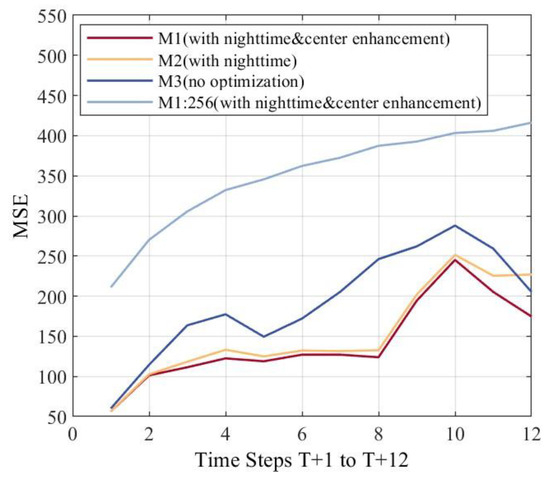
Figure A2.
Comparative Analysis of MSE Trends Across Different Spatial Ranges and the Impact of Nighttime Data Training and Center Enhancement Strategy on Prediction Stability. The x-axis represents prediction time (T + 1, T + 2……T + 12) with a time step of 15 min, and the y-axis indicates the MSE of predicted COT surrounding the target site.
Appendix A.3
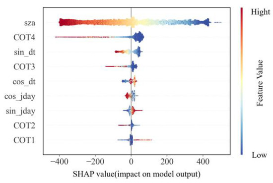
Figure A3.
SHAP Values for Interpreting the LightGBM Model. The y-axis ranks the features by the sum of their SHAP values across all samples. The x-axis represents the SHAP values, which indicate the distribution of each feature’s impact on the model output. Each point corresponds to a single sample, with samples stacked vertically. The color denotes the feature value, where red indicates high values and blue indicates low values. For instance, the first row shows that high sza (red) has a negative impact on the prediction, while low sza (blue) has a positive impact.
Appendix A.4
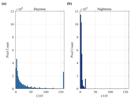
Figure A4.
The COT Distributions for the Day and Night Subsets. The x-axis represents COT value, and the y-axis indicates the counts of corresponding COT value of all COT images (384 × 384) around the ABQ site. Figures (a) and (b) respectively show the histograms of COT distribution for daytime and nighttime.
Appendix A.5
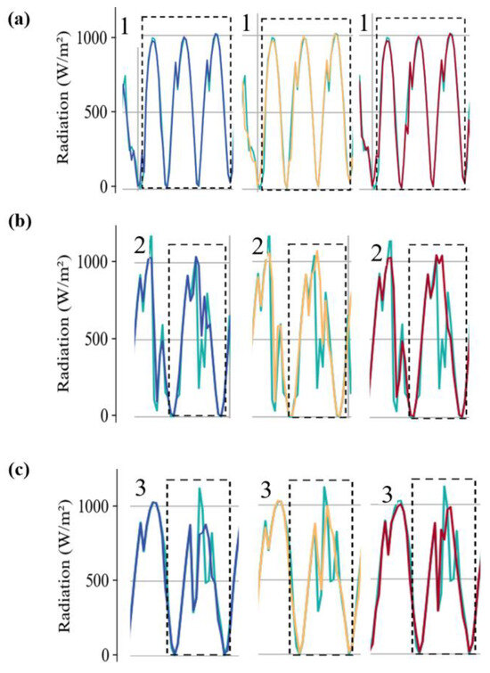
Figure A5.
Separate Figures Focusing on the Three Boxes. (a), (b), and (c) represent the details of the curves in Box 1, Box 2, and Box 3, respectively. From left to right are the predicted and actual radiation curves for the next 1 h, 2 h, and 3 h. The light green color represents the true value of radiation, while the blue, yellow, and red curves respectively represent the radiation prediction values for 1 h, 2 h, and 3 h in the future.
Appendix B
Appendix B.1
Specifically, we get the reference model prediction values using Equation (A1).
To determine the value of α, we use the last observation of COT in all cases of the training set to obtain the SSI estimation values using LighGBM for all 12 future time steps as the regular persistence (). The three-year (2020–2022) average SSI at the corresponding time points is used as the climatological values (). We then minimize the RMSE between the reference model prediction and the actual values to determine the value of α.
After determining α, we apply this formula to the testing set cases. For each case in the testing set, we use the last observation of COT to obtain the regular persistence from the LightGBM model and use the three-year average SSI at that time point as the climatological value. By plugging these values into the formula, we obtain the reference model’s SSI forecast values for each cases.
References
- Filonchyk, M.; Peterson, M.P.; Zhang, L.; Hurynovich, V.; He, Y. Greenhouse Gases Emissions and Global Climate Change: Examining the Influence of CO2, CH4, and N2O. Sci. Total Environ. 2024, 935, 173359. [Google Scholar] [CrossRef]
- International Energy Agency (IEA). Electricity 2025. Available online: https://www.iea.org/reports/electricity-2025 (accessed on 6 June 2025).
- Jacobson, M.Z.; Delucchi, M.A. Providing All Global Energy with Wind, Water, and Solar Power, Part I: Technologies, Energy Resources, Quantities and Areas of Infrastructure, and Materials. Energy Policy 2011, 39, 1154–1169. [Google Scholar] [CrossRef]
- Kosmopoulos, P.G.; Kazadzis, S.; Taylor, M.; Raptis, P.I.; Keramitsoglou, I.; Kiranoudis, C.; Bais, A.F. Assessment of Surface Solar Irradiance Derived from Real-Time Modelling Techniques and Verification with Ground-Based Measurements. Atmos. Meas. Tech. 2018, 11, 907–924. [Google Scholar] [CrossRef]
- Nanou, S.I.; Papakonstantinou, A.G.; Papathanassiou, S.A. A Generic Model of Two-Stage Grid-Connected PV Systems with Primary Frequency Response and Inertia Emulation. Electr. Power Syst. Res. 2015, 127, 186–196. [Google Scholar] [CrossRef]
- Shah, R.; Mithulananthan, N.; Bansal, R.C.; Ramachandaramurthy, V.K. A Review of Key Power System Stability Challenges for Large-Scale PV Integration. Renew. Sustain. Energy Rev. 2015, 41, 1423–1436. [Google Scholar] [CrossRef]
- Wang, F.; Zhen, Z.; Mi, Z.; Sun, H.; Su, S.; Yang, G. Solar Irradiance Feature Extraction and Support Vector Machines Based Weather Status Pattern Recognition Model for Short-Term Photovoltaic Power Forecasting. Energy Build. 2015, 86, 427–438. [Google Scholar] [CrossRef]
- Luo, X.; Zhang, D.; Zhu, X. Deep Learning Based Forecasting of Photovoltaic Power Generation by Incorporating Domain Knowledge. Energy 2021, 225, 120240. [Google Scholar] [CrossRef]
- Khan, J.; Arsalan, M.H. Solar Power Technologies for Sustainable Electricity Generation—A Review. Renew. Sustain. Energy Rev. 2016, 55, 414–425. [Google Scholar] [CrossRef]
- Markovics, D.; Mayer, M.J. Comparison of Machine Learning Methods for Photovoltaic Power Forecasting Based on Numerical Weather Prediction. Renew. Sustain. Energy Rev. 2022, 161, 112364. [Google Scholar] [CrossRef]
- Ma, W.; Wu, J.; Yan, P. Ultra-Short Term Solar Irradiance Prediction Considering Satellite Cloud Images. In Proceedings of the 2024 7th International Conference on Energy, Electrical and Power Engineering (CEEPE), Yangzhou, China, 26–28 April 2024; pp. 1371–1377. [Google Scholar]
- Zhang, Y.; Liang, S.; He, T. Estimation of Land Surface Downward Shortwave Radiation Using Spectral-Based Convolutional Neural Network Methods: A Case Study From the Visible Infrared Imaging Radiometer Suite Images. IEEE Trans. Geosci. Remote Sens. 2022, 60, 4414415. [Google Scholar] [CrossRef]
- Huang, G.; Li, Z.; Li, X.; Liang, S.; Yang, K.; Wang, D.; Zhang, Y. Estimating Surface Solar Irradiance from Satellites: Past, Present, and Future Perspectives. Remote Sens. Environ. 2019, 233, 111371. [Google Scholar] [CrossRef]
- Huang, G.; Ma, M.; Liang, S.; Liu, S.; Li, X. A LUT-Based Approach to Estimate Surface Solar Irradiance by Combining MODIS and MTSAT Data: Estimating SSI Combining MODIS and MTSAT. J. Geophys. Res. 2011, 116, D22201. [Google Scholar] [CrossRef]
- Mora-López, L.L.; Sidrach-de-Cardona, M. Multiplicative ARMA Models to Generate Hourly Series of Global Irradiation. Sol. Energy 1998, 63, 283–291. [Google Scholar] [CrossRef]
- Liu, Z.-F.; Li, L.-L.; Tseng, M.-L.; Lim, M.K. Prediction Short-Term Photovoltaic Power Using Improved Chicken Swarm Optimizer—Extreme Learning Machine Model. J. Clean. Prod. 2020, 248, 119272. [Google Scholar] [CrossRef]
- Huang, C.; Yang, M. Memory Long and Short Term Time Series Network for Ultra-Short-Term Photovoltaic Power Forecasting. Energy 2023, 279, 127961. [Google Scholar] [CrossRef]
- Xiao, X.; Mo, H.; Zhang, Y.; Shan, G. Meta-ANN—A Dynamic Artificial Neural Network Refined by Meta-Learning for Short-Term Load Forecasting. Energy 2022, 246, 123418. [Google Scholar] [CrossRef]
- Cao, J.C.; Cao, S.H. Study of Forecasting Solar Irradiance Using Neural Networks with Preprocessing Sample Data by Wavelet Analysis. Energy 2006, 31, 3435–3445. [Google Scholar] [CrossRef]
- Aprillia, H.; Yang, H.-T.; Huang, C.-M. Statistical Load Forecasting Using Optimal Quantile Regression Random Forest and Risk Assessment Index. IEEE Trans. Smart Grid 2021, 12, 1467–1480. [Google Scholar] [CrossRef]
- Hao, D.; Asrar, G.R.; Zeng, Y.; Zhu, Q.; Wen, J.; Xiao, Q.; Chen, M. Estimating Hourly Land Surface Downward Shortwave and Photosynthetically Active Radiation from DSCOVR/EPIC Observations. Remote Sens. Environ. 2019, 232, 111320. [Google Scholar] [CrossRef]
- Bae, K.Y.; Jang, H.S.; Sung, D.K. Hourly Solar Irradiance Prediction Based on Support Vector Machine and Its Error Analysis. IEEE Trans. Power Syst. 2016, 32, 935–945. [Google Scholar] [CrossRef]
- Liu, L.; Liu, F.; Zheng, Y. A Novel Ultra-Short-Term PV Power Forecasting Method Based on DBN-Based Takagi-Sugeno Fuzzy Model. Energies 2021, 14, 6447. [Google Scholar] [CrossRef]
- Caldas, M.; Alonso-Suárez, R. Very Short-Term Solar Irradiance Forecast Using All-Sky Imaging and Real-Time Irradiance Measurements. Renew. Energy 2019, 143, 1643–1658. [Google Scholar] [CrossRef]
- Yang, H.; Kurtz, B.; Nguyen, D.; Urquhart, B.; Chow, C.W.; Ghonima, M.; Kleissl, J. Solar Irradiance Forecasting Using a Ground-Based Sky Imager Developed at UC San Diego. Sol. Energy 2014, 103, 502–524. [Google Scholar] [CrossRef]
- Siddiqui, T.A.; Bharadwaj, S.; Kalyanaraman, S. A Deep Learning Approach to Solar-Irradiance Forecasting in Sky-Videos. In Proceedings of the 2019 IEEE Winter Conference on Applications of Computer Vision (WACV), Waikoloa Village, HI, USA, 7–9 January 2019; pp. 2166–2174. [Google Scholar]
- Kosmopoulos, P.; Kouroutsidis, D.; Papachristopoulou, K.; Raptis, P.I.; Masoom, A.; Saint-Drenan, Y.-M.; Blanc, P.; Kontoes, C.; Kazadzis, S. Short-Term Forecasting of Large-Scale Clouds Impact on Downwelling Surface Solar Irradiation. Energies 2020, 13, 6555. [Google Scholar] [CrossRef]
- Si, Z.; Yang, M.; Yu, Y.; Ding, T. Photovoltaic Power Forecast Based on Satellite Images Considering Effects of Solar Position. Appl. Energy 2021, 302, 117514. [Google Scholar] [CrossRef]
- Straub, N.; Karalus, S.; Herzberg, W.; Lorenz, E. Satellite-Based Solar Irradiance Forecasting: Replacing Cloud Motion Vectors by Deep Learning. Sol. RRL 2024, 8, 2400475. [Google Scholar] [CrossRef]
- Chiu, J.C.; Huang, C.; Marshak, A.; Slutsker, I.; Giles, D.M.; Holben, B.N.; Knyazikhin, Y.; Wiscombe, W.J. Cloud Optical Depth Retrievals from the Aerosol Robotic Network (AERONET) Cloud Mode Observations. J. Geophys. Res. 2010, 115, 2009JD013121. [Google Scholar] [CrossRef]
- Wang, Y.; Wu, H.; Zhang, J.; Gao, Z.; Wang, J.; Yu, P.S.; Long, M. PredRNN: A Recurrent Neural Network for Spatiotemporal Predictive Learning. IEEE Trans. Pattern Anal. Mach. Intell. 2023, 45, 2208–2225. [Google Scholar] [CrossRef]
- Michael, C. GOES-R Series Product Definition and Users’ Guide (PUG) Volume 5: Level 2+ Products. Available online: https://www.goes-r.gov/products/docs/PUG-L2+-vol5.pdf (accessed on 6 June 2025).
- Hasler, A.F.; Shenk, W.E.; Skillman, W.C. Wind Estimates from Cloud Motions: Results from Phases I, II and III of an In Situ Aircraft Verification Experiment. J. Appl. Meteorol. 1977, 16, 812–815. [Google Scholar] [CrossRef]
- Rossow, W.B.; Knapp, K.R.; Young, A.H. International Satellite Cloud Climatology Project: Extending the Record. J. Clim. 2022, 35, 141–158. [Google Scholar] [CrossRef]
- Ke, G.; Meng, Q.; Finley, T.; Wang, T.; Chen, W.; Ma, W.; Ye, Q.; Liu, T.-Y. LightGBM: A Highly Efficient Gradient Boosting Decision Tree. In Proceedings of the 31st International Conference on Neural Information Processing Systems; Long Beach, CA, USA, 4–9 December 2017, pp. 3149–3157.
- Gan, M.; Pan, S.; Chen, Y.; Cheng, C.; Pan, H.; Zhu, X. Application of the Machine Learning LightGBM Model to the Prediction of the Water Levels of the Lower Columbia River. J. Mar. Sci. Eng. 2021, 9, 496. [Google Scholar] [CrossRef]
- Wang, Y.; Wang, T. Application of Improved LightGBM Model in Blood Glucose Prediction. Appl. Sci. 2020, 10, 3227. [Google Scholar] [CrossRef]
- Zhao, X.; Liu, Y.; Zhao, Q. Improved LightGBM for Extremely Imbalanced Data and Application to Credit Card Fraud Detection. IEEE Access 2024, 12, 159316–159335. [Google Scholar] [CrossRef]
- Yang, D.; Alessandrini, S.; Antonanzas, J.; Antonanzas-Torres, F.; Badescu, V.; Beyer, H.G.; Blaga, R.; Boland, J.; Bright, J.M.; Coimbra, C.F.M.; et al. Verification of Deterministic Solar Forecasts. Sol. Energy 2020, 210, 20–37. [Google Scholar] [CrossRef]
- Marchesoni-Acland, F.; Herrera, A.; Mozo, F.; Camiruaga, I.; Castro, A.; Alonso-Suárez, R. Deep Learning Methods for Intra-Day Cloudiness Prediction Using Geostationary Satellite Images in a Solar Forecasting Framework. Sol. Energy 2023, 262, 111820. [Google Scholar] [CrossRef]
- Yang, D. Making Reference Solar Forecasts with Climatology, Persistence, and Their Optimal Convex Combination. Sol. Energsy 2019, 193, 981–985. [Google Scholar] [CrossRef]
- Platnick, S.; King, M.D.; Ackerman, S.A.; Menzel, W.P.; Baum, B.A.; Riedi, J.C.; Frey, R.A. The MODIS Cloud Products: Algorithms and Examples from Terra. IEEE Trans. Geosci. Remote Sens. 2003, 41, 459–473. [Google Scholar] [CrossRef]
- Su, X.; Li, T.; An, C.; Wang, G. Prediction of Short-Time Cloud Motion Using a Deep-Learning Model. Atmosphere 2020, 11, 1151. [Google Scholar] [CrossRef]
- Aicardi, D.; Musé, P.; Alonso-Suárez, R. A Comparison of Satellite Cloud Motion Vectors Techniques to Forecast Intra-Day Hourly Solar Global Horizontal Irradiation. Sol. Energy 2022, 233, 46–60. [Google Scholar] [CrossRef]
- Obiora, C.N.; Ali, A. Effective Implementation of Convolutional Long Short-Term Memory (ConvLSTM) Network in Forecasting Solar Irradiance. In Proceedings of the IECON 2021—47th Annual Conference of the IEEE Industrial Electronics Society, Toronto, ON, Canada, 13–16 October 2021; pp. 1–5. [Google Scholar]
- Farnebäck, G. Two-Frame Motion Estimation Based on Polynomial Expansion. In Image Analysis; Bigun, J., Gustavsson, T., Eds.; Lecture Notes in Computer Science; Springer: Berlin/Heidelberg, Germany, 2003; Volume 2749, pp. 363–370. ISBN 978-3-540-40601-3. [Google Scholar]
- Hasan, R.; Siddique, T.; Rahman, M.S.; Kabir, M.A. LSTM-Based Deep Learning Model for Solar Irradiance Prediction Across Diverse Climate Zones. In Proceedings of the 2025 IEEE Kansas Power and Energy Conference (KPEC), Manhattan, KS, USA, 24–25 April 2025; pp. 1–6. [Google Scholar]
Disclaimer/Publisher’s Note: The statements, opinions and data contained in all publications are solely those of the individual author(s) and contributor(s) and not of MDPI and/or the editor(s). MDPI and/or the editor(s) disclaim responsibility for any injury to people or property resulting from any ideas, methods, instructions or products referred to in the content. |
© 2025 by the authors. Licensee MDPI, Basel, Switzerland. This article is an open access article distributed under the terms and conditions of the Creative Commons Attribution (CC BY) license (https://creativecommons.org/licenses/by/4.0/).