Abstract
Simultaneous Localization and Mapping (SLAM) is a critical technology for robot intelligence. Compared to cameras, Light Detection and Ranging (LiDAR) sensors achieve higher accuracy and stability in indoor environments. However, LiDAR can only capture the geometric structure of the environment, and LiDAR-based SLAM often fails in scenarios with insufficient geometric features or highly similar structures. Furthermore, low-cost mechanical LiDARs, constrained by sparse point cloud density, are particularly prone to odometry drift along the Z-axis, especially in environments such as tunnels or long corridors. To address the localization issues in such scenarios, we propose a forward-enhanced SLAM algorithm. Utilizing a 16-line LiDAR and a monocular camera, we construct a dense colored point cloud input and apply an efficient multi-modal feature extraction algorithm based on centroid distance to extract a set of feature points with significant geometric and color features. These points are then optimized in the back end based on constraints from points, lines, and planes. We compare our method with several classic SLAM algorithms in terms of feature extraction, localization, and elevation constraint. Experimental results demonstrate that our method achieves high-precision real-time operation and exhibits excellent adaptability to indoor environments with similar structures.
1. Introduction
Robotics technology is advancing rapidly, with SLAM (Simultaneous Localization and Mapping) being the foundation for mobile robots to achieve global localization, map building, and path planning in unknown environments. As robot operating scenarios and tasks become increasingly complex, the joint operation of multiple sensors to provide more accurate localization and mapping results for robots is a direction of common research interest.
Currently, there are many sensors used in SLAM, mainly divided into active sensors and passive sensors. Active sensors mainly include LiDAR and cameras, while passive sensors include GNSS and UWB, etc. The Global Navigation Satellite System (GNSS) is widely used due to its ability to provide accurate positioning information [1]. However, current satellite signals cannot penetrate buildings, making GNSS unsuitable for indoor positioning [2]. Devices like Ultra-Wideband (UWB) have precise indoor positioning capabilities but require the installation of base stations, which are costly and complex to deploy [3]. LiDAR and cameras, as the two main self-contained sensors in SLAM, have imaging that aligns with human intuition and perform well indoors and outdoors. Therefore, these two sensors are currently the main research directions in the SLAM field.
However, LiDAR can only capture the geometric information of the environment, which may lead to positioning or mapping issues, especially in environments like tunnels or long corridors that lack a distinct geometric structure or have repeated geometric patterns. These similar geometric structures and their proximity in the map can lead to errors in the frame-to-frame matching and frame-to-map matching processes of LiDAR odometry, ultimately resulting in significant confusion in odometry estimation and rendering the map construction unusable. In these narrow environments, the close proximity of the sensor to the walls results in highly dense laser points on the walls. Many algorithms tend to ignore features that are too close, too dense, and structurally homogeneous to improve processing speed and stability. Moreover, operators following behind in narrow environments further exacerbate the errors in LiDAR odometry, preventing the full utilization of LiDAR’s 360° field of view and long-range detection advantages in such settings. Additionally, the 16-line LiDAR point cloud provides much sparser information in the vertical direction compared to the horizontal direction. This disparity causes many SLAM algorithms relying on LiDAR to exhibit good accuracy on the horizontal plane but significant vertical deviations, often resulting in odometry or mapping curling along the z-axis. In contrast, due to different principles of feature extraction, the forward-facing monocular cameras usually perform well in such environments. However, they also have inherent issues such as high computational load and scale ambiguity. Therefore, effectively integrating the advantages of both sensors to develop a lightweight LiDAR–vision fusion SLAM algorithm in narrow and structurally similar environments is a key focus of current research.
To address the above challenges, we propose a novel method for rapidly fusing 3D LiDAR and monocular camera information, achieving precise and robust localization in indoor long corridor environments with similar structures. Our design offers the following contributions:
- ①
- We design a forward-projection and interpolation strategy to construct dense colored point clouds from sparse 16-line LiDAR scans and monocular images. This enhancement improves vertical resolution and front-view coverage, enabling scan-to-map pose estimation and reducing z-axis drift in long narrow indoor scenes.
- ②
- We introduce a lightweight multi-modal feature extraction algorithm based on centroid distances, which jointly considers geometric and photometric saliency. A dynamic radius adjustment mechanism is incorporated to adapt neighborhood size according to the point’s distance from the LiDAR sensor, ensuring stable feature quality under varying point densities.
- ③
- We incorporate a feature reliability weighting strategy into the back-end joint optimization, assigning higher weights to original LiDAR points and lower weights to interpolated or color-enhanced points. The proposed system is validated in challenging indoor environments and demonstrates strong localization accuracy and robustness.
The rest of the article is organized as follows: Related work is reviewed in Section 2. The overview of the proposed system is presented in Section 3. Section 4 presents the detailed algorithm descriptions applied in our system, followed by experimental results in Section 5. Finally, Section 6 provides a summary of this paper.
2. Related Work
LiDAR odometry has undergone years of development. With its increasingly widespread application and diverse usage scenarios, there is a growing demand for the stability of LiDAR SLAM algorithms.
In the field of 3D LiDAR SLAM, LOAM (Lidar Odometry and Mapping in Real-Time) is one of the earliest breakthrough works [4]. Many current LiDAR SLAM algorithms have been developed based on LOAM, progressively establishing the fundamental processes of point cloud registration, front-end odometry, back-end optimization, and loop closure detection. LeGO-LOAM builds on this foundation by adding ground constraints, significantly reducing odometry and mapping errors in the vertical direction [5]. FLOAM simplifies motion correction and odometry optimization by directly using scan-to-map optimization, which markedly reduces computation time [6]. LOAM-Livox is the first to apply this method to solid-state LiDAR, implementing targeted optimizations for its unique scanning pattern [7].
In terms of LiDAR and IMU fusion, LIO-SAM is one of the most popular LiDAR-IMU fusion algorithms today [8], and it integrates edge and plane residual errors with IMU residual errors to construct a tightly-coupled pose graph optimization method. FAST-LIO [9] and FAST-LIO2 [10] have also successfully demonstrated the ability to achieve high-precision positioning by fusing LiDAR and IMU through filtering methods.
In the realm of LiDAR and visual fusion SLAM, methods like DEMO [11] and LIMO [12] leverage LiDAR points to provide depth information for RGB images, reducing scale uncertainty in visual odometry. Additionally, stereo vision systems [13,14] and RGB-D algorithms such as BAD-SLAM [15], GS-SLAM [16,17], and a photometric LiDAR/RGB-D bundle adjustment method [18] can generate dense colored point clouds, providing a rich combination of geometric and texture information. VLOAM [19], DVL-SLAM [20,21], and TVL-SAM [22] combine the laser odometry factor with the visual odometry factor or semantic information [23] to enhance system accuracy and robustness.
Deep learning has been widely adopted for LiDAR odometry and localization. LO-Net demonstrates end-to-end odometry learning with a mask-weighted geometric consistency constraint [24]. L3-Net advances learning-based LiDAR localization using cost-volume reasoning and temporal modeling [25]. CAE-LO further explores a fully unsupervised pipeline for interest-point detection and feature description [26]. DVLO integrates visual and LiDAR cues via local-to-global feature fusion and bi-directional structure alignment to improve robustness [27].
Currently, numerous works [28,29] have comprehensively reviewed the advancements and technical challenges in multi-sensor fusion methods involving LiDAR and other sensors, providing valuable insights and significant references for further exploration in this field. However, LiDAR still suffers from point cloud degradation in structurally similar environments. When numerous similar geometric structures are present, it significantly increases the uncertainty in pose estimation. Therefore, achieving precise localization in such scenes is a key challenge in LiDAR SLAM. In the field of pure LiDAR SLAM, the detection of point cloud degradation is commonly achieved by assessing the uncertainty of point cloud matching between two frames [30] and examining the geometric features of the point cloud [31,32]. In terms of fusion processing, LiDAR–IMU integration is a widely adopted approach, exemplified by methods such as FAST-LIO [9] and FAST-LIO2 [10]. FF-LINS [33] further improves frame-to-frame state estimation for solid-state LiDAR–inertial systems, enhancing consistency and accuracy. IMU trajectory estimation is not affected by the specific environment, making it an effective complement to compensate for LiDAR degradation. Nevertheless, compared to IMU, the fusion of LiDAR and cameras offers additional advantages by integrating both geometric and visual information, which provides richer scene interpretation and can further enhance localization accuracy. The input information from LiDAR and vision can complement each other, combining geometric and textural information, which is a common approach to solving localization problems in similar environments [34,35]. Recent work [36] has demonstrated the practical advantages and challenges of applying such fusion in large-scale indoor environments, particularly under low-texture and long-range conditions. Additionally, using the intensity information from the LiDAR itself as a new image input achieves the advantage of modal fusion when using only pure LiDAR data [37]. The addition of UWB can provide precise absolute positioning for LiDAR odometry [3], but its initial setup is cumbersome, making it difficult to use directly in unfamiliar environments. Some work integrates LiDAR, IMU, and camera in a tightly coupled manner to enhance system robustness and mapping consistency [38,39]. Building on this idea, LVIO-Fusion [40] directly fuses LiDAR and camera measurements with IMU data, achieving high accuracy and robustness in geometrically degenerate and texture-less environments. More recently, a detection-first tightly coupled LiDAR–visual–inertial SLAM framework prioritizes stable object detection before multi-sensor fusion, mitigating dynamic interference and geometric degeneracy to enhance localization robustness [41]. However, this also poses more challenges for the quality of front-end data. Other approaches focus on loop closure detection in similar scenes [42,43], using the combined information from multiple sensors to address matching errors in loop closure detection in similar scenes. This approach allows for the holistic optimization of odometry.
3. System Overview
The overall system structure is presented in Figure 1. The SLAM framework in this paper utilizes a 16-line LiDAR and a monocular camera as the core sensors for localization and mapping. By fusing the monocular camera with the LiDAR, the system achieves fast, robust, and stable localization in indoor environments with similar geometric features at low cost. The front-end input consists of hybrid dense point clouds generated from fused LiDAR and camera data, where both geometric and color information are considered for feature extraction. An improved centroid distance feature extraction method is employed to capture multimodal feature points. After applying joint constraints based on geometry and color, the back-end optimization utilizes a scan-to-map approach, ensuring accurate and real-time localization while fully integrating information from both sensors.
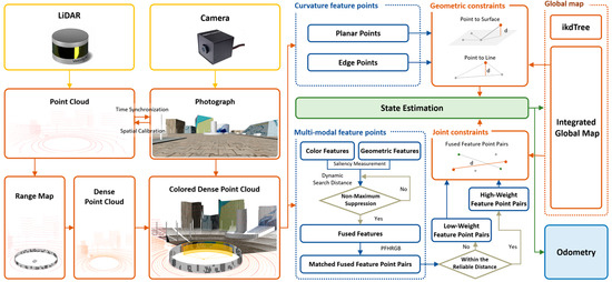
Figure 1.
System overview of the proposed method. This paper constructs a colored dense laser point cloud using inputs from a 16-line LiDAR and a monocular camera. We extract feature points by combining geometric and color characteristics and ultimately use scan-to-map joint optimization to obtain precise odometry information.
4. Methodology
4.1. Hybrid Dense Point Cloud Construction Based on Range Map
Laser point clouds are typically unordered. Traditional methods [4] assign indices to each laser beam based on their angular information to facilitate efficient search. In the proposed method, we utilize range maps generated from LiDAR scans to achieve point cloud densification and coloring. Taking the Velodyne 16-line LiDAR as an example, the resolution of the constructed strip range map is 16 × 1800. By leveraging the calibrated intrinsic and extrinsic parameters, we align the pixel data with the point cloud and employ spherical projection combined with interpolation to enhance density. This process results in the construction of a dense colored 128 × 1800 range map, which is ultimately transformed back into a dense colored point cloud for input, as illustrated in Figure 2.
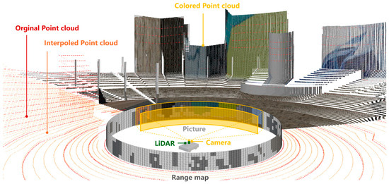
Figure 2.
The image illustrates the process of constructing a range map from the LiDAR point cloud and integrating it with a monocular camera to generate a dense colored point cloud. The red points represent the original LiDAR point cloud, while the orange points denote the interpolated LiDAR points. By overlaying the camera image, the LiDAR points within the camera’s field of view are assigned to the corresponding color at each position.
For each scanned point , where , we first convert it from Cartesian coordinates to spherical coordinates:
where denotes the range, is the azimuth, and represents the elevation component, and then map the spherical coordinates to image coordinates by the spherical projection function . The formula is as follows:
where and are the width and height of the range image, respectively. is the vertical field-of-view of the LiDAR sensor.
The next step is the densification of the point cloud, with a focus on solving localization challenges in indoor environments such as long corridors. Compared to complex and dynamic settings like urban outdoor roads, these long corridor scenarios are relatively straightforward and typically characterized by structured geometrically simple surfaces such as walls. In such environments, we adopt a direct bilinear interpolation approach to ensure real-time performance. This method enhances environmental information without imposing significant computational overhead. The formula for bilinear interpolation is as follows:
where is the distance function corresponding to the point, and are the four known points around the interpolation point.
Finally, for coloring the point cloud, precise calibration of both the LiDAR and monocular camera is conducted. In this paper, Zhang’s method [44] is employed to determine the intrinsic parameters of the camera, enabling the accurate rectification of camera images. Additionally, LiDAR–camera joint calibration [45] is conducted to establish the relative spatial alignment between the LiDAR and monocular camera, enabling data integration and point correspondence for coloring. The coloring and extrinsic transformation formulas are as follows:
where and are the rotation matrix and translation vector representing the extrinsic transformation from the LiDAR coordinate frame to the camera coordinate frame. are camera intrinsic parameters, are focal lengths, and are optical centers.
4.2. Search-Radius-Optimized Centroid-Based Feature Point Extraction
In LiDAR processing, a common approach to point cloud extraction involves computing the curvature of each point to distinguish between planar and edge features based on the curvature magnitude. However, in environments with high levels of repetition, purely geometric LiDAR odometry often leads to mismatches, causing confusion in localization and mapping. Current LiDAR–visual odometry fusion algorithms typically run LiDAR odometry and visual odometry independently before merging the two odometries into a final output. However, these methods not only require significant computational resources, but also fail to fully leverage the fusion of visual color features with LiDAR geometric features. Considering the incorporation of colored point clouds in the previous chapter, this paper proposes extracting mixed features containing both geometric and color information from dense colored point clouds.
First, we consider the geometric properties of a colored point cloud. For a point in a colored point cloud , includes geometric components and color components . For a given set of point cloud data in a specific coordinate system, the centroid of the point cloud remains invariant regardless of the rotation and translation of the point cloud [46]. The relative positions of all points in the point cloud with respect to the geometric center of the point cloud are also invariant.
Inspired by the method proposed by Teng et al. [46], When traversing each point in the colored point cloud, for a given point cloud set , for each query point , the query point searches the neighborhood point set within a spherical region defined by a search radius to calculate the geometric centroid of the spherical region:
where is the set of neighboring points in the spherical space around query point with a radius of , is the centroid of the point cloud , correspond to the geometric coordinates of each point, and is the distance from the query point to the point cloud centroid, serving as a measure of geometric saliency. As indicated in Figure 3, it can be observed that the farther the query point is from the centroid, the more likely it is to be a corner point with distinct geometric structures.
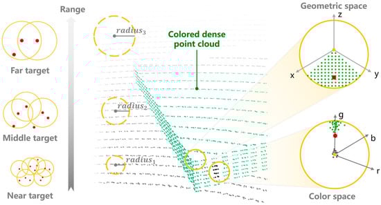
Figure 3.
A schematic diagram of feature point extraction based on centroid distance. The yellow point represents the current point, and the yellow circle represents the spherical search area with a search radius. The red point represents the centroid within the spherical search area. In the geometric space, the farther the search point is from the geometric centroid, the more likely it is an edge corner point; conversely, it is a planar point. In the color space, the farther the search point is from the color centroid, the more significant the color change at that point. As the distance increases, the LiDAR point cloud becomes increasingly sparse. By increasing the search radius according to the distance variation, the utilization of point cloud features can be effectively enhanced.
LiDAR point cloud density inherently decreases with increasing distance from the sensor, resulting in a non-uniform distribution of spatial information. Although densification techniques can alleviate this to some extent, point clouds at greater distances remain significantly sparser compared to those nearby. As a result, applying a fixed-radius neighborhood search across the entire range leads to suboptimal outcomes: a small radius may fail to capture sufficient context in distant regions, while a large radius near the sensor can introduce excessive and redundant neighbors, increasing computational cost without meaningful benefit.
To address this limitation, we integrate a dynamically adjustable search radius into the centroid-distance-based feature extraction framework. By scaling the radius according to each point’s distance from the LiDAR origin, the method effectively adapts to variations in point cloud density across different sensing ranges. Specifically, let denote a point in the point cloud, and represent its Euclidean distance to the LiDAR coordinate origin . The search radius is then defined as follows:
where and are empirically determined scaling and offset parameters. This formulation ensures that the search radius remains appropriately sized, being large enough for distant points to maintain sufficient neighborhood coverage, while remaining small enough for nearby points to prevent redundant computations. This linear model balances feature coverage and computational efficiency across varying point cloud densities.
To further constrain the search range and improve robustness, we apply lower and upper bounds to the radius, denoted as and . The final adaptive search radius is computed as follows.
This dynamic radius strategy allows the neighborhood size to adapt smoothly with distance, ensuring sufficient feature support in sparse long-range regions while maintaining efficiency in dense close-range areas.
Next, we extend our consideration to the color space of the colored point cloud. In the color space, treating the color coordinates equivalently to the geometric coordinates allows us to find the color centroid in a similar way to the geometric centroid in the above geometric corner point query method, as illustrated in the “color space” of Figure 3. We search for corner points with drastic color changes within a varying search radius along with the changing distance of the point cloud. The basic formula is as follows:
where is the color centroid of and is the color distance from the query point to the point cloud’s color centroid, serving as a measure of color saliency. The values , , denote the RGB color components of the query point , which are obtained from the fused dense colored point cloud constructed by aligning the LiDAR data with the monocular camera image. , , correspond to the RGB values of the color centroid, calculated as the average of the RGB values of all neighboring points in the local region. Since color values range from 0 to 255 as integers, we use the L1 norm to measure whether a point has significant color changes within its neighborhood. A point is considered to have drastic color changes when it is far from most points in color space.
Finally, appropriate feature point selection is performed. We choose a suitable geometric distance threshold and color distance threshold to remove feature points with insignificant geometric and color features. Among the remaining feature points, we select those with the best geometric and color characteristics based on saliency measurement. For example, on a flat floor, where geometric features are mostly planar, we would select texture points with distinct colors, such as brick joints. In cases where all points have similar colors, we prioritize geometric changes. By applying the nonlinear suppression algorithm to select the points with the highest combined saliency in the neighborhood, a multi-modal key point set can be obtained, as shown in Figure 4.
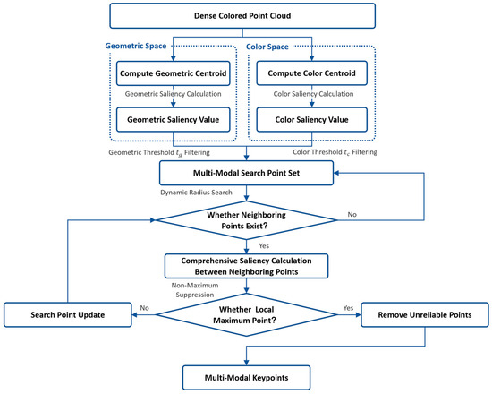
Figure 4.
Structure of multi-modal key point extraction.
Additionally, following the traditional point cloud feature extraction methods, unreliable points are removed. Points hidden behind objects can lead to incorrect edge point extraction. Points at the edge of the camera’s field of view (FoV) can also reduce the reliability of extracted features. When the incident angle is close to 0 or 180 degrees, the laser spot becomes larger, causing the laser beam’s ranging to be the average distance of all points within the spot, rather than the distance to a specific point. This leads to inaccurate ranging. Therefore, after removing these points, we obtain the final fused feature points.
4.3. Geometric and Color Joint Optimization
For each input of the dense colored point cloud scan, multimodal key points incorporating both color and geometric relationships are extracted using the centroid-distance-based method described in the previous section. For global localization optimization, we adopt a scan-to-map matching approach, aligning the current frame with the global map. The global feature map consists of a multimodal feature map and traditional edge-plane feature maps, which are updated and maintained separately. Key points are described using Point Feature Histogram RGB (PFHRGB) descriptors [47], and we use ikd-tree for nearest neighbor search to enhance search efficiency. Simultaneously, edge and plane features are extracted by calculating the curvature of each point. The extracted multimodal and geometric feature points then undergo joint iterative pose optimization, considering local smoothness, through scan-to-map operations to obtain the final pose.
To ensure robust feature matching in the re-colored dense point cloud, we incorporate a confidence-based weighting strategy that accounts for the reliability differences among feature points. After projecting the point cloud onto the range map and performing interpolation to densify it, we label whether each point originates from the original 16-line LiDAR scan or is generated through interpolation. For interpolated points, we further compute the minimum vertical distance to their nearest original scan points in the range map, using this as an indicator of proximity to true sensor measurements. Feature points that are closer to the original scan lines are considered more reliable, as they are directly observed rather than synthesized. These points are assigned higher weights during optimization to reflect their greater trustworthiness. In contrast, interpolated points that lie farther from the original data are assigned lower weights, as they may suffer from geometric or photometric distortions introduced during interpolation.
Let the set of hybrid feature points extracted from the current frame be , and the corresponding successfully matched feature points in the map be . The assigned weights based on reliability distance are represented as . Therefore, the residual calculation formula is as follows:
where and represent the rotation matrix and translation vector from the current frame to the global map, is the index of the current point, and is the total number of points in the current frame’s point cloud.
Secondly, edge points and planar points are considered. Edge features are extracted from the point cloud of the current frame and stored as , where . For each edge feature point, we search for five nearby edge points in the global edge map using ikd-tree. Based on the geometric center of these five points and eigenvalue decomposition, the center and direction vector of the global line are determined. We select two points on the line as and , where is the half-length offset along the line direction from the center point and is used to define reference points on the global line for distance computation. The residual function is then constructed based on the distance from the current frame point to the global line. The residual function can be formulated as follows.
Similar to the edge feature points, for a point in the planar feature set of the current frame, we search for five nearest points in the global planar map. Using these five nearest points, the normal vector of the constructed global plane is determined as . Based on the point-to-plane distance, the residual is then formulated as follows.
After obtaining the residual function for color and geometric constraints, we can formulate the entire optimization problem as follows:
where and represent the weights for different features, respectively, enabling the system to adapt flexibly to diverse environmental conditions. These parameters are empirically determined based on performance evaluations across multiple validation sequences and are chosen to achieve a balanced trade-off between robustness and accuracy by emphasizing the contribution of more reliable features. We then employ the Gaussian–Newton method to perform the optimization.
5. Experiment
5.1. Experiment Setup
To validate the reliability of our algorithm, we conducted experiments in both a simulation environment and on a public benchmark dataset. The simulation environment represents a comprehensive urban setting, modeled in Blender and imported into Gazebo. It features densely built street environments as well as long corridor environments characterized by geometric features. The simulated hardware setup consists of a Velodyne 16-line LiDAR operating at 10 Hz and a virtual monocular RGB camera with a resolution of 1980 × 800, also running at 10 Hz.
For real-world dataset validation, we utilized public benchmark datasets. Considering that our method focuses on addressing the practicality of low-cost hardware in challenging environments such as long indoor corridors, widely used datasets like KITTI lack corresponding indoor scenarios. Therefore, to evaluate the proposed method, we employed the publicly available S3E dataset [39]. S3E is a large-scale multimodal dataset collected by a fleet of unmanned ground vehicles following four specifically designed collaborative trajectory paradigms. It includes seven outdoor and five indoor sequences, each exceeding 200 s. For our experiments, we selected the temporally synchronized and spatially calibrated data from the Velodyne VLP-16 Puck LiDAR (Velodyne Lidar Inc., San Jose, CA, USA) and the HikRobot MV-CS050-10GC GigE left-eye camera (Hangzhou Hikrobot Technology Co., Ltd., Hangzhou, China). The camera resolution is 1224 × 1024, and both sensors operate at a frame rate of 10 Hz.
For the selection of scenarios from the public dataset, we chose specific scenes for comparison. Portions of the dataset corresponding to the Teaching Building, Laboratory, Library, and Square were selected, representing four experimental scenarios: long indoor corridor, indoor rooms, long-distance outdoor environment, and geometrically similar outdoor environment. Figure 5 illustrates the comparison between the simulation environment and the real-world environments from the S3E dataset. For LiDAR localization, environments with unclear geometric features pose significant challenges. Therefore, this paper focuses on fusion localization using visual assistance in narrow and structurally similar indoor environments. To make the experimental results more comparable, we limited the maximum scanning radius of the LiDAR. Additionally, experiments in outdoor environments validate the general applicability of the proposed algorithm. The following sections detail the experimental setup and methodology.
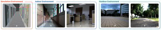
Figure 5.
Simulation environment and real dataset environment demonstration; (a) represents the simulation environment, which includes a 70 m long corridor to verify the reliability of our proposed algorithm in similar environments. Four groups of datasets were selected for the real-world environment, corresponding to different working conditions: long similar indoor environment (b), indoor rooms environment (c), long-distance outdoor environment (d), and similar outdoor environment (e).
5.2. Hybrid Dense Point Cloud Construction
The original LiDAR point cloud is 16-line, which provides sparse information for similar indoor environments. This is particularly true in the vertical direction, where the density of the point cloud is much lower than in the horizontal direction. As a result, many SLAM algorithms relying on LiDAR exhibit good accuracy on the plane but significant vertical deviations, often leading to odometry or mapping curling along the z-axis. Compared to outdoor environments, indoor environments are simpler in terms of both the number of obstacles and the geometric structure of the space. In closer proximity, dense point clouds can cover most of the space with fewer blind spots. Therefore, enhancing the information on the z-axis in indoor environments through point cloud interpolation is a rapid and stable method. Moreover, depth estimation using monocular cameras is currently complex and suffers from scale uncertainty. By using LiDAR coloring for point cloud depth estimation, we can complement the weaknesses of both sensors. The results of the interpolated and colored point cloud are shown in Figure 6. The colored dense point clouds provide more information compared to the sparse 16-line point clouds. The interpolated point cloud maintains the original LiDAR points’ layout, interpolating the 16-line points to a 128-line point cloud. This enhances the utilization of point cloud information and adds color information to the geometric data, increasing the reliability of localization in similar environments.
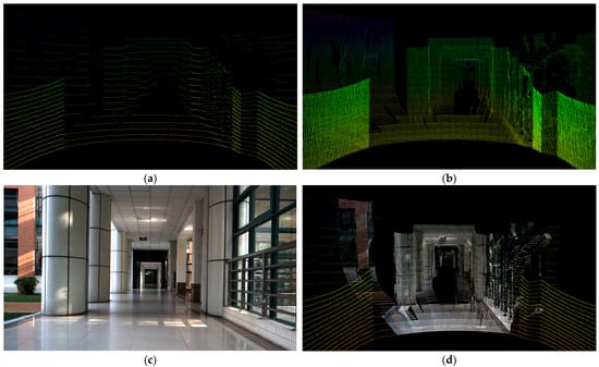
Figure 6.
LiDAR densification and coloring demonstration images: (a) is the original 16-line LiDAR point cloud, (b) is the densified point cloud, (c) is the original photograph from the monocular camera, and (d) is the densified and colored point cloud. The colored dense point cloud retains precise geometric and color features.
5.3. Results of Feature Point Extraction
To verify the effectiveness of the centroid distance feature extraction method with variable search distance in LiDAR, we selected several classic feature extraction algorithms for images or point clouds, such as the LOAM feature and ORB feature, for comparison. We chose scenes with clear geometry or color features and analyzed the performance of different algorithms in different environments. As shown in Figure 7, Figure 7a–c correspond to the same indoor scene, while Figure 7d–f correspond to the same long corridor scene. In the indoor environment where both geometric and texture features are well defined, LOAM’s point cloud features can identify a large number of plane feature points and edge points, especially accurately extracting edge points at corners. However, LOAM can only classify flat surfaces as plane points and does not effectively respond to patterns on boxes or seams on the floor. In contrast, ORB identifies salient points based on color differences in camera images, effectively recognizing areas with color inconsistencies as feature points. Our method combines the strengths of both approaches, extracting feature points that capture clear geometric structures and recognizing texture details. The LiDAR and vision fusion feature extraction algorithm used in this paper integrates the advantages of both geometric and color features. It can extract matching points based on color when the plane points are dense. Therefore, as shown in Figure 7f, the mixed feature points are primarily concentrated in areas with color variations and clear geometric structures, such as mural images, picture frames, columns, and floor tile seams. This provides accurate positional information in geometrically similar environments.
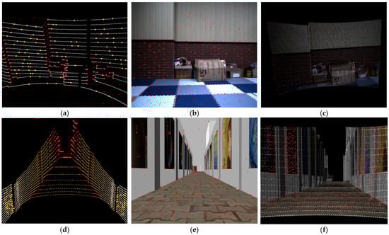
Figure 7.
The result of feature extraction: (a,d) show LOAM features extracted from 16-line point clouds, where red points represent edge features and yellow points represent plane features, (b,e) are camera frames with red points indicating ORB features, and (c,f) are mixed dense point clouds, with red points representing mixed features. Our feature extraction algorithm comprehensively considers both geometric and color information.
5.4. Localization Accuracy on the Simulation Dataset
To validate the odometry performance improvement of our proposed fusion algorithm compared to classical SLAM algorithms in similar indoor environments, we selected several algorithms for comparison. Among pure LiDAR SLAM algorithms, we chose LOAM, FLOAM, and LeGO-SLAM, while for monocular visual SLAM, we selected ORB-SLAM2. For LiDAR–vision-fusion-based localization, due to the limited availability of open-source options, we employed VLOAM, which combines a monocular camera with a mechanical LiDAR as a reference.
As shown in Figure 8, in the street area with clear scene hierarchy and abundant geometric features, the performance of the algorithms is generally consistent. At the starting point, the trajectories of the algorithms almost overlap, demonstrating good accuracy in the initial stage. However, once entering the long corridor area, the differences between the odometry algorithms become apparent. To further analyze their performance in this challenging environment, we extracted the planar trajectories from the long corridor region and presented a detailed comparison in Figure 9. Among them, FLOAM exhibits the most severe point cloud degradation, with the odometry in the tunnel measuring only half of the true value. This is related to its scan-to-map odometry matching approach and the sacrifice of some convergence iterations for computational efficiency. While it maintains good localization in the geometrically rich street environment, the reduced iteration speed becomes a disadvantage when geometric features decrease, resulting in significant degradation. LOAM and LeGO-LOAM perform better but still show noticeable degradation in the long corridor. Since this study only utilizes a monocular camera, the classical visual algorithm ORB-SLAM2 can only determine scale through the initial two-frame estimation from the monocular camera. As shown in the figure, while the odometry performs well in the long corridor area, there is a noticeable scale estimation error.
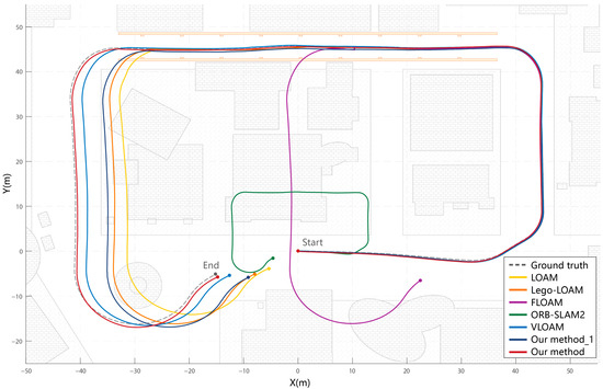
Figure 8.
Comparison of trajectory errors for simulation environment. “Our method_1” is the trajectory obtained by interpolating the point cloud without coloring at the front end. “Our method” is the complete algorithm proposed in this paper. The comparison between the two verifies the effectiveness of hybrid dense point cloud in this specific environment. Other comparison algorithms exhibit varying degrees of degradation, while the algorithm proposed in this paper can effectively overcome the degradation of point clouds caused by long-distance similar environments.
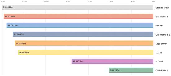
Figure 9.
Comparison of odometry performance in the long corridor region. The proposed method demonstrates the closest trajectory to the ground truth in tunnel distance estimation.
Among the compared methods, VLOAM demonstrated the best overall performance in general environments, benefiting from joint optimization of visual and LiDAR information. It achieved high localization accuracy in structured non-corridor areas. However, in the long corridor scenario evaluated in this study, VLOAM still exhibited noticeable odometry errors, particularly in elevation, due to the sparse vertical resolution of the LiDAR and the lack of robust constraints in repetitive structures. Our Method_1, which employs only LiDAR point cloud interpolation without incorporating color information, improved point density and offered partial stabilization. Nevertheless, it failed to eliminate the fundamental drift, confirming that increased spatial resolution alone is insufficient in repetitive environments. Its trajectory still showed substantial deviation in the XY plane, with no significant improvement over other LiDAR-only methods.
In contrast, the full version of our proposed method, which integrates both geometric and photometric cues, achieved the most accurate and robust trajectory. By incorporating texture information from the monocular camera, the distinctiveness of key points was enhanced, enabling more reliable data association even in geometrically ambiguous scenes. Moreover, vertical interpolation effectively mitigated elevation inconsistencies, resulting in overall superior performance in both horizontal and vertical localization.
These results confirm that the proposed fusion strategy significantly enhances SLAM robustness and accuracy in geometrically degenerate environments, particularly in long indoor corridors where traditional LiDAR- or vision-only systems are prone to drift and failure.
In the elevation variation graph for this scene, as shown in Figure 10, our proposed method also demonstrates an advantage. One primary reason that LiDAR SLAM systems experience z-axis curling during localization and mapping is the excessive sparsity of point clouds in the vertical direction. By increasing the information along the z-axis during point cloud interpolation, vertical deviations are better suppressed. Among the algorithms, LOAM exhibits significant z-axis estimation errors. LeGO-LOAM, with ground constraints, performs well but exhibits a maximum to minimum error range difference exceeding 3 m. VLOAM performs well overall; however, it experiences elevation jumps in the long corridor region, which is one of the contributing factors to odometry degradation observed in the planar trajectory results. Our proposed method increases the amount of information in the elevation direction, maintains the error range difference within 3 m even without ground constraints, and achieves superior z-axis localization performance compared to many LiDAR SLAM methods, with a significant improvement in computational efficiency.
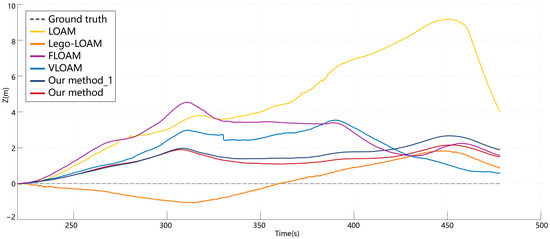
Figure 10.
Comparison of cumulative elevation errors in the simulation environment. Our proposed method shows significant improvement, with cumulative errors second only to LeGO-LOAM, which has ground constraints. In terms of absolute deviations between the maximum and minimum values, our method outperforms both LeGO-LOAM and VLOAM.
Table 1 presents the Absolute Errors of various SLAM algorithms in the simulation environment. For ORB-SLAM2, due to the scale uncertainty inherent in monocular vision, the evaluation results are obtained using scale alignment. Among the various compared odometry methods, including LiDAR-based, vision-based, and fusion-based approaches, our proposed method maintains a high level across multiple evaluation metrics.

Table 1.
Absolute Errors in simulation environment (m).
5.5. Runtime Evaluation on the Simulation Dataset
Table 2 shows the average processing time per frame for several odometry algorithms. The testing environment is based on ROS Noetic and Ubuntu 20.04, with the test computer equipped with an i5-8500 CPU. The processing time is measured from the initiation of data input to the output of the estimated odometry. As shown in the table, SLAM based on 16-line LiDAR runs faster than vision-based solutions. Although monocular vision is highly efficient in front-end feature extraction, its back-end SLAM processing, particularly the bundle adjustment, is more time-consuming. The proposed method combines both LiDAR and vision data inputs, yet the overall processing time is comparable to that of the purely vision-based ORB-SLAM2. This efficiency stems from the rapid extraction of central distance features and the streamlined frame-to-map matching process, offering a computational advantage over VLOAM. Experimental results in simulated environments demonstrate that the proposed approach enhances localization accuracy in structurally similar environments while preserving real-time performance.
Table 2.
Time consumption of different algorithms (ms).
5.6. Results of Public Benchmark Dataset in Indoor Environment
To validate the effectiveness of our proposed approach, we conducted experiments using the public benchmark dataset S3E, focusing on indoor scenarios such as long corridors and laboratory rooms. The planar trajectory and elevation comparisons are illustrated in Figure 11 and Figure 12. Due to the narrow and sharp-turning nature of these environments, the monocular visual odometry of ORB-SLAM2 often failed to maintain tracking and was, therefore, excluded from the final comparison.
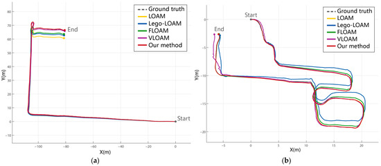
Figure 11.
Comparison of trajectory errors for real environments. Our proposed method maintains stability and achieves good results in two environments; especially in similar indoor environments (a), it can effectively solve the degradation problem. In the laboratory environment (b), our method remains consistently stable even when other classic algorithms exhibit noticeable drift.
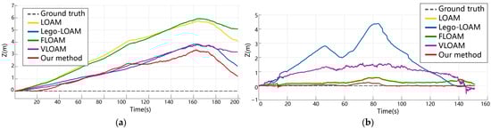
Figure 12.
Comparison of cumulative elevation errors in real environments. in similar indoor environments (a), our cumulative error is second only to LeGO-LOAM; but, in the indoor laboratory scene (b), LeGO-LOAM produced a large error, while our method still performed well.
In the long corridor scenario (Figure 11a and Figure 12a), characterized by repetitive geometric structures and minimal texture, all pure LiDAR-based algorithms (e.g., LOAM, LeGO-LOAM, FLOAM) exhibited varying degrees of drift or degradation, particularly in elevation. This is attributed to the reduced diversity in geometric features, which leads to unstable feature extraction and erroneous scan-to-map associations. Although LeGO-LOAM incorporates ground constraints to enhance z-axis accuracy, its performance still declined in the absence of distinct ground features. FLOAM suffered the most severe drift due to its reliance on sparse scan-to-map optimization. In contrast, VLOAM, which leverages camera information, achieved improved stability. However, its performance degraded in extended repetitive sections, particularly on the elevation axis. Our proposed method outperformed all competitors in both trajectory accuracy and elevation stability by leveraging dense colored point clouds and multimodal feature constraints. Notably, the integration of color-based features contributed to more reliable localization in geometrically ambiguous regions.
In the laboratory room scenario (Figure 11b and Figure 12b), all algorithms performed relatively well in the initial stages due to the presence of more diverse structures. However, LeGO-LOAM exhibited significant drift in the latter half, and VLOAM showed oscillatory behavior in the z-axis trajectory. This highlights their limitations in handling environments with occlusions and irregular geometry. In contrast, our method maintained trajectory consistency and demonstrated the smallest cumulative error, even without relying on loop closure. The robust performance across both structured corridors and cluttered rooms suggests that our method can adapt to a variety of indoor environments.
Overall, these comparative results highlight that, while traditional LiDAR and visual odometry methods perform adequately under certain conditions, their robustness is challenged in complex or repetitive indoor scenes. Our proposed fusion-based method achieves higher accuracy and stability across different types of indoor environments by effectively combining geometric and photometric information. The results also underscore the potential of the proposed approach in enhancing localization performance in scenarios where single-modality methods struggle.
Table 3 shows the results of the quantitative analysis of the absolute positional error. In indoor room environments, the RMSE differences among the various algorithms are relatively minor, with only LeGO-LOAM and VLOAM showing instability in the laboratory scene. In contrast, in the long indoor corridor scenario, which represents geometrically similar environments, the errors caused by point cloud degradation are more pronounced. The two algorithms incorporating visual information performed comparatively well. Our proposed method demonstrated the best performance across both indoor environments, showing a significant improvement over the other algorithms and proving the practical feasibility of the approach.
Table 3.
Absolute Errors (RMSE) in public benchmark dataset in indoor environment (m).
5.7. Results of Public Benchmark Dataset in Outdoor Environments
In outdoor environments, the openness of the scenes and the complexity of features present certain limitations for the dense LiDAR algorithm proposed in this paper, resulting in generally moderate depth estimation accuracy.
In the outdoor building environment (Figure 13a and Figure 14a), the presence of clear structural features resulted in generally consistent planar trajectory accuracy across all algorithms during the initial stage. However, given the larger scene scale and longer trajectories in outdoor settings, differences became apparent after two turns. VLOAM, which incorporates constraints from both LiDAR and camera measurements, achieved slightly better performance in the xy-plane compared with pure LiDAR-based algorithms. In terms of elevation accuracy, LOAM exhibited the largest drift. Although LeGO-LOAM benefited from ground constraints, providing a certain advantage, its cumulative elevation error over a long run of more than 400 m remained at the 10 m level, showing no significant gap from VLOAM or our method. While the proposed approach did not yield notable accuracy improvements in this outdoor environment due to its inherent limitations, the use of dense colored point clouds still contributed to better z-axis constraints.
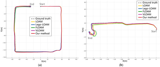
Figure 13.
Comparison of trajectory errors for real outdoor environments. In the outdoor building environment (a), all algorithms performed similarly at this scale. In the outdoor path environment (b), LOAM and FLOAM exhibited notable errors. Although our method did not achieve the best performance, it maintained a competitive level in both outdoor scenarios, demonstrating its general applicability.
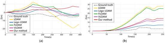
Figure 14.
Comparison of cumulative elevation errors in real outdoor environments. In the outdoor building environment (a), LOAM exhibited large errors. In the outdoor path environment (b), LeGO-LOAM achieved the best performance, followed by VLOAM and our method, while FLOAM and LOAM showed the largest cumulative errors. Leveraging its ground constraints, LeGO-LOAM demonstrated clear advantages in both scenarios, whereas VLOAM and our method performed significantly better than the purely LiDAR-based LOAM and FLOAM.
In the outdoor tree-lined path environment (Figure 13b and Figure 14b), more pronounced trajectory differences were observed. For planar accuracy, LOAM and FLOAM performed the worst, showing substantial deviations from the other three algorithms at the endpoint. The elevation results exhibited even larger disparities: LeGO-LOAM, aided by ground constraints, achieved the best performance and VLOAM and our method ranked next, whereas LOAM and FLOAM accumulated elevation errors exceeding 25 m over a 200 m trajectory, indicating a significant reduction in reliability in large-scale long-distance scenarios.
Table 4 presents the quantitative analysis of absolute positional errors in outdoor environments. The results are consistent with our trajectory analysis, further supporting this observation. In the building environment, considering both planar and elevation accuracy over long-distance runs, VLOAM achieved the lowest RMSE. In the path environment, LeGO-LOAM delivered excellent performance in both planar and elevation accuracy, attaining the best RMSE as expected. Although the proposed method has not been specifically optimized for open outdoor environments, it still outperformed purely LiDAR-based algorithms, demonstrating a certain degree of generalization capability in outdoor scenarios.
Table 4.
Absolute Errors (RMSE) in public benchmark dataset in outdoor environment (m).
6. Conclusions
In this paper, we address the issue of inaccurate LiDAR localization in indoor environments with similar structures by proposing a forward-enhanced SLAM algorithm that fuses LiDAR and monocular vision. For point cloud registration, we combine LiDAR and camera data to construct a hybrid dense point cloud, effectively constraining vertical deviations while increasing the information content of the input data. For feature extraction, we use a centroid-distance-based method to accurately and efficiently extract feature points that represent combined saliency in both geometric and color spaces from the colorized point cloud, employing dynamic search distances based on LiDAR characteristics. In the optimization part, we use three types of feature matching—points, lines, and planes—and enhance LiDAR odometry performance significantly in geometrically similar regions through fast scan-to-map optimization.
In future work, we plan to improve the LiDAR interpolation algorithm to enhance the accuracy of front-end data and incorporate LiDAR bundle adjustment into the back-end optimization to establish more reliable constraints. To further improve adaptability and robustness, especially in complex outdoor environments, we also intend to develop adaptive weighting mechanisms that adjust the contributions of geometric and color features based on scene characteristics or feature confidence.
Author Contributions
Conceptualization, Z.Z. and W.J.; methodology, C.G.; software, Z.Z. and Y.L.; validation, Z.Z., Y.L. and X.Z.; formal analysis, Z.Z.; investigation, Y.L. and X.Z.; resources, W.J. and C.G.; data curation, Z.Z.; writing—original draft preparation, Z.Z.; writing—review and editing, C.G. and W.J.; visualization, Z.Z. and X.Z.; supervision, C.G. and W.J.; project administration, Z.Z.; funding acquisition, C.G. and W.J. All authors have read and agreed to the published version of the manuscript.
Funding
This research is supported and funded by the Major Program (JD) of Hubei Province (No.2023BAA025), the Major Science and Technology Program for Hubei Province (No. 2022AAA002), and the Major Science and Technology Program for Hubei Province (No. 2022AAA009).
Data Availability Statement
The raw data supporting the conclusions of this article will be made available by the authors on request.
Conflicts of Interest
The authors declare no conflicts of interest.
References
- Jiang, W.; Liu, T.; Chen, H.; Song, C.; Chen, Q.; Geng, T. Multi-Frequency Phase Observable-Specific Signal Bias Estimation and Its Application in the Precise Point Positioning with Ambiguity Resolution. GPS Solut. 2023, 27, 4. [Google Scholar] [CrossRef]
- Jiang, W.; Chen, Y.; Chen, Q.; Chen, H.; Pan, Y.; Liu, X.; Liu, T. High Precision Deformation Monitoring with Integrated GNSS and Ground Range Observations in Harsh Environment. Measurement 2022, 204, 112179. [Google Scholar] [CrossRef]
- Zhou, H.; Yao, Z.; Lu, M. Lidar/UWB Fusion Based SLAM With Anti-Degeneration Capability. IEEE Trans. Veh. Technol. 2021, 70, 820–830. [Google Scholar] [CrossRef]
- Zhang, J.; Singh, S. LOAM: Lidar Odometry and Mapping in Real-Time. In Proceedings of the Robotics: Science and Systems X, Robotics: Science and Systems Foundation, Berkeley, CA, USA, 12–16 July 2014. [Google Scholar]
- Shan, T.; Englot, B. LeGO-LOAM: Lightweight and Ground-Optimized Lidar Odometry and Mapping on Variable Terrain. In Proceedings of the 2018 IEEE/RSJ International Conference on Intelligent Robots and Systems (IROS), Madrid, Spain, 1–5 October 2018; pp. 4758–4765. [Google Scholar]
- Wang, H.; Wang, C.; Chen, C.-L.; Xie, L. F-LOAM: Fast LiDAR Odometry and Mapping. In Proceedings of the 2021 IEEE/RSJ International Conference on Intelligent Robots and Systems (IROS), Prague, Czech Republic, 27 September–1 October 2021; pp. 4390–4396. [Google Scholar]
- Lin, J.; Zhang, F. Loam_livox: A Fast, Robust, High-Precision LiDAR Odometry and Mapping Package for LiDARs of Small FoV. In Proceedings of the 2020 IEEE International Conference on Robotics and Automation (ICRA), Paris, France, 31 May–31 August 2020. [Google Scholar]
- Shan, T.; Englot, B.; Meyers, D.; Wang, W.; Ratti, C.; Rus, D. LIO-SAM: Tightly-Coupled Lidar Inertial Odometry via Smoothing and Mapping. In Proceedings of the 2020 IEEE/RSJ International Conference on Intelligent Robots and Systems (IROS), Las Vegas, NV, USA, 25–29 October 2020; pp. 5135–5142. [Google Scholar]
- Xu, W.; Zhang, F. FAST-LIO: A Fast, Robust LiDAR-Inertial Odometry Package by Tightly-Coupled Iterated Kalman Filter. IEEE Robot. Autom. Lett. 2021, 6, 3317–3324. [Google Scholar] [CrossRef]
- Xu, W.; Cai, Y.; He, D.; Lin, J.; Zhang, F. FAST-LIO2: Fast Direct LiDAR-Inertial Odometry. IEEE Trans. Robot. 2022, 38, 2053–2073. [Google Scholar] [CrossRef]
- Zhang, J.; Kaess, M.; Singh, S. A Real-Time Method for Depth Enhanced Visual Odometry. Auton. Robot. 2017, 41, 31–43. [Google Scholar] [CrossRef]
- Graeter, J.; Wilczynski, A.; Lauer, M. LIMO: Lidar-Monocular Visual Odometry. In Proceedings of the 2018 IEEE/RSJ International Conference on Intelligent Robots and Systems (IROS), Madrid, Spain, 1–5 October 2018. [Google Scholar]
- Campos, C.; Elvira, R.; Rodríguez, J.J.G.; Montiel, J.M.; Tardós, J.D. ORB-SLAM3: An Accurate Open-Source Library for Visual, Visual–Inertial, and Multimap SLAM. IEEE Trans. Robot. 2021, 37, 1874–1890. [Google Scholar] [CrossRef]
- Pire, T.; Baravalle, R.; D’Alessandro, A.; Civera, J. Real-Time Dense Map Fusion for Stereo SLAM. Robotica 2018, 36, 1510–1526. [Google Scholar] [CrossRef]
- Schops, T.; Sattler, T.; Pollefeys, M. BAD SLAM: Bundle Adjusted Direct RGB-D SLAM. In Proceedings of the 2019 IEEE/CVF Conference on Computer Vision and Pattern Recognition (CVPR), Long Beach, CA, USA, 15–20 June 2019; pp. 134–144. [Google Scholar]
- Yan, C.; Qu, D.; Xu, D.; Zhao, B.; Wang, Z.; Wang, D.; Li, X. GS-SLAM: Dense Visual SLAM with 3D Gaussian Splatting. In Proceedings of the IEEE/CVF Conference on Computer Vision and Pattern Recognition 2024, Seattle, WA, USA, 16–22 June 2024. [Google Scholar]
- Zhao, H.; Guan, W.; Lu, P. LVI-GS: Tightly Coupled LiDAR–Visual–Inertial SLAM Using 3-D Gaussian Splatting. IEEE Trans. Instrum. Meas. 2025, 74, 7504810. [Google Scholar] [CrossRef]
- Di Giammarino, L.; Giacomini, E.; Brizi, L.; Salem, O.; Grisetti, G. Photometric LiDAR and RGB-D Bundle Adjustment. IEEE Robot. Autom. Lett. 2023, 8, 4362–4369. [Google Scholar] [CrossRef]
- Zhang, J.; Singh, S. Visual-Lidar Odometry and Mapping: Low-Drift, Robust, and Fast. In Proceedings of the 2015 IEEE International Conference on Robotics and Automation (ICRA), Seattle, WA, USA, 26–30 May 2015; pp. 2174–2181. [Google Scholar]
- Shin, Y.-S.; Park, Y.S.; Kim, A. DVL-SLAM: Sparse Depth Enhanced Direct Visual-LiDAR SLAM. Auton. Robot. 2020, 44, 115–130. [Google Scholar] [CrossRef]
- Shin, Y.-S.; Park, Y.S.; Kim, A. Direct Visual SLAM Using Sparse Depth for Camera-LiDAR System. In Proceedings of the 2018 IEEE International Conference on Robotics and Automation (ICRA), Brisbane, QLD, Australia, 21–25 May 2018; pp. 5144–5151. [Google Scholar]
- Chou, C.-C.; Chou, C.-F. Efficient and Accurate Tightly-Coupled Visual-Lidar SLAM. IEEE Trans. Intell. Transp. Syst. 2022, 23, 14509–14523. [Google Scholar] [CrossRef]
- Chen, W.; Shang, G.; Ji, A.; Zhou, C.; Wang, X.; Xu, C.; Li, Z.; Hu, K. An Overview on Visual SLAM: From Tradition to Semantic. Remote Sens. 2022, 14, 3010. [Google Scholar] [CrossRef]
- Li, Q.; Chen, S.; Wang, C.; Li, X.; Wen, C.; Cheng, M.; Li, J. LO-Net: Deep Real-Time Lidar Odometry. In Proceedings of the IEEE/CVF Conference on Computer Vision and Pattern Recognition 2019, Long Beach, CA, USA, 15–20 June 2019; pp. 8473–8482. [Google Scholar]
- Lu, W.; Zhou, Y.; Wan, G.; Hou, S.; Song, S. L3-Net: Towards Learning Based LiDAR Localization for Autonomous Driving. In Proceedings of the IEEE/CVF Conference on Computer Vision and Pattern Recognition 2019, Long Beach, CA, USA, 15–20 June 2019; pp. 6389–6398. [Google Scholar]
- Yin, D.; Zhang, Q.; Liu, J.; Liang, X.; Wang, Y.; Maanpää, J.; Ma, H.; Hyyppä, J.; Chen, R. CAE-LO: LiDAR Odometry Leveraging Fully Unsupervised Convolutional Auto-Encoder for Interest Point Detection and Feature Description. arXiv 2020, arXiv:2001.01354. [Google Scholar]
- Liu, J.; Zhuo, D.; Feng, Z.; Zhu, S.; Peng, C.; Liu, Z.; Wang, H. DVLO: Deep Visual-LiDAR Odometry with Local-to-Global Feature Fusion and Bi-Directional Structure Alignment. In European Conference on Computer Vision; Springer Nature: Cham, Switzerland, 2024. [Google Scholar]
- Zhu, J.; Li, H.; Zhang, T. Camera, LiDAR, and IMU Based Multi-Sensor Fusion SLAM: A Survey. Tsinghua Sci. Technol. 2024, 29, 415–429. [Google Scholar] [CrossRef]
- Zhang, Y.; Shi, P.; Li, J. 3D LiDAR SLAM: A Survey. Photogramm. Rec. 2024, 39, 457–517. [Google Scholar] [CrossRef]
- Tuna, T.; Nubert, J.; Nava, Y.; Khattak, S.; Hutter, M. X-ICP: Localizability-Aware LiDAR Registration for Robust Localization in Extreme Environments. IEEE Trans. Robot. 2024, 40, 452–471. [Google Scholar] [CrossRef]
- Gao, H.; Zhang, X.; Fang, Y.; Yuan, J. A Line Segment Extraction Algorithm Using Laser Data Based on Seeded Region Growing. Int. J. Adv. Robot. Syst. 2018, 15, 172988141875524. [Google Scholar] [CrossRef]
- Ji, M.; Shi, W.; Cui, Y.; Liu, C.; Chen, Q. Adaptive Denoising-Enhanced LiDAR Odometry for Degeneration Resilience in Diverse Terrains. IEEE Trans. Instrum. Meas. 2024, 73, 8501715. [Google Scholar] [CrossRef]
- Tang, H.; Zhang, T.; Niu, X.; Wang, L.; Wei, L.; Liu, J. FF-LINS: A Consistent Frame-to-Frame Solid-State-LiDAR-Inertial State Estimator. IEEE Robot. Autom. Lett. 2023, 8, 8525–8532. [Google Scholar] [CrossRef]
- Lin, J.; Zhang, F. R3LIVE: A Robust, Real-Time, RGB-Colored, LiDAR-Inertial-Visual Tightly-Coupled State Estimation and Mapping Package. In Proceedings of the 2022 International Conference on Robotics and Automation (ICRA), Philadelphia, PA, USA, 23–27 May 2022; pp. 10672–10678. [Google Scholar]
- Huang, S.-S.; Ma, Z.-Y.; Mu, T.-J.; Fu, H.; Hu, S.-M. Lidar-Monocular Visual Odometry Using Point and Line Features. In Proceedings of the 2020 IEEE International Conference on Robotics and Automation (ICRA), Paris, France, 31 May–31 August 2020; pp. 1091–1097. [Google Scholar]
- Ress, V.; Zhang, W.; Skuddis, D.; Haala, N.; Soergel, U. SLAM for Indoor Mapping of Wide Area Construction Environments. arXiv 2024, arXiv:2404.17215. [Google Scholar] [CrossRef]
- Du, W.; Beltrame, G. Real-Time Simultaneous Localization and Mapping with LiDAR Intensity. arXiv 2023, arXiv:2301.09257. [Google Scholar]
- Boche, S.; Laina, S.B.; Leutenegger, S. Tightly-Coupled LiDAR-Visual-Inertial SLAM and Large-Scale Volumetric Occupancy Mapping. In Proceedings of the 2024 IEEE International Conference on Robotics and Automation (ICRA), Yokohama, Japan, 13–17 May 2024. [Google Scholar]
- Wen, T.; Fang, Y.; Lu, B.; Zhang, X.; Tang, C. LIVER: A Tightly Coupled LiDAR-Inertial-Visual State Estimator With High Robustness for Underground Environments. IEEE Robot. Autom. Lett. 2024, 9, 2399–2406. [Google Scholar] [CrossRef]
- Zhang, H.; Du, L.; Bao, S.; Yuan, J.; Ma, S. LVIO-Fusion:Tightly-Coupled LiDAR-Visual-Inertial Odometry and Mapping in Degenerate Environments. IEEE Robot. Autom. Lett. 2024, 9, 3783–3790. [Google Scholar] [CrossRef]
- Xu, X.; Hu, J.; Zhang, L.; Cao, C.; Yang, J.; Ran, Y.; Tan, Z.; Xu, L.; Luo, M. Detection-First Tightly-Coupled LiDAR-Visual-Inertial SLAM in Dynamic Environments. Measurement 2025, 239, 115506. [Google Scholar] [CrossRef]
- Zhou, Z.; Guo, C.; Pan, Y.; Li, X.; Jiang, W. A 2-D LiDAR-SLAM Algorithm for Indoor Similar Environment With Deep Visual Loop Closure. IEEE Sens. J. 2023, 23, 14650–14661. [Google Scholar] [CrossRef]
- Wang, X.; Zheng, S.; Lin, X.; Zhang, Q.; Liu, X. Robust Loop Closure Detection and Relocalization with Semantic-Line Graph Matching Constraints in Indoor Environments. Int. J. Appl. Earth Obs. Geoinf. 2024, 129, 103844. [Google Scholar] [CrossRef]
- Zhang, Z. A Flexible New Technique for Camera Calibration. IEEE Trans. Pattern Anal. Mach. Intell. 2000, 22, 1330–1334. [Google Scholar] [CrossRef]
- Zhou, L.; Li, Z.; Kaess, M. Automatic Extrinsic Calibration of a Camera and a 3D LiDAR Using Line and Plane Correspondences. In Proceedings of the 2018 IEEE/RSJ International Conference on Intelligent Robots and Systems (IROS), Madrid, Spain, 1–5 October 2018; pp. 5562–5569. [Google Scholar]
- Teng, H.; Chatziparaschis, D.; Kan, X.; Roy-Chowdhury, A.K.; Karydis, K. Centroid Distance Keypoint Detector for Colored Point Clouds. In Proceedings of the 2023 IEEE/CVF Winter Conference on Applications of Computer Vision (WACV), Waikoloa, HI, USA, 2–7 January 2023; pp. 1196–1205. [Google Scholar]
- Alexandre, L.A. Set Distance Functions for 3D Object Recognition. In Progress in Pattern Recognition, Image Analysis, Computer Vision, and Applications; Ruiz-Shulcloper, J., Sanniti Di Baja, G., Eds.; Lecture Notes in Computer Science; Springer: Berlin/Heidelberg, Germany, 2013; Volume 8258, pp. 57–64. ISBN 978-3-642-41821-1. [Google Scholar]
Disclaimer/Publisher’s Note: The statements, opinions and data contained in all publications are solely those of the individual author(s) and contributor(s) and not of MDPI and/or the editor(s). MDPI and/or the editor(s) disclaim responsibility for any injury to people or property resulting from any ideas, methods, instructions or products referred to in the content. |
© 2025 by the authors. Licensee MDPI, Basel, Switzerland. This article is an open access article distributed under the terms and conditions of the Creative Commons Attribution (CC BY) license (https://creativecommons.org/licenses/by/4.0/).