Abstract
Monitoring salt marsh vegetation in the Yellow River Delta (YRD) wetland is the basis of wetland research, which is of great significance for the further protection and restoration of wetland ecological functions. In the existing remote sensing technologies for wetland salt marsh vegetation classification, the object-oriented classification method effectively produces landscape patches similar to wetland vegetation and improves the spatial consistency and accuracy of the classification. However, the vegetation classes of the YRD are mixed with uneven distribution, irregular texture, and significant color variation. In order to solve the problem, this study proposes a fine-scale classification of dominant vegetation communities using color-enhanced aerial images. The color information is used to extract the color features of the image. Various features including spectral features, texture features and vegetation features are extracted from the image objects and used as inputs for four machine learning classifiers: random forest (RF), support vector machine (SVM), k-nearest neighbor (KNN) and maximum likelihood (MLC). The results showed that the accuracy of the four classifiers in classifying vegetation communities was significantly improved by adding color features. RF had the highest OA and Kappa coefficients of 96.69% and 0.9603. This shows that the classification method based on color enhancement can effectively distinguish between vegetation and non-vegetation and extract each vegetation type, which provides an effective technical route for wetland vegetation classification in aerial imagery.
1. Introduction
Coastal wetlands are an important type of wetland and are a natural transition from land to sea; they are one of the most productive and dynamic ecosystems on the planet due to the strong interaction between terrestrial rivers and coastal oceans [1,2]. They play an irreplaceable and important role in protecting the ecological environment, regulating climate, controlling soil erosion, and developing the economy and society [3,4,5]. However, coastal wetlands are under intense pressure from rising sea levels [6], coastal erosion [7], land reclamation [8], invasive species [9], and reduced sediment discharges from major rivers [10]. In developing countries such as China, many anthropogenic activities and environmental factors associated with rapid population growth and economic development have threatened coastal wetlands [11,12,13]. As the main primary producer and the main body of ecosystem functions, vegetation is the most active part of wetland biological components and plays an important role in water conservation, climate regulation, biodiversity maintenance.
The Yellow River Delta (YRD) has the most complete, extensive and youngest estuarine wetland ecosystem in China, and it has created about 5400 km2 of land since it was incorporated into the Bohai Sea in 1855 [14,15]. In the wetlands of the YRD, communities such as Suaeda salsa (S.s), Phragmites australis (P.a) and Tamarix chinensis (T.c) are the most typical vegetation communities [16]. The classification of wetland salt marsh vegetation can provide a scientific basis for the protection and restoration of wetland ecological functions in the YRD. First, there are significant differences in the carbon sequestration benefits of different salt marsh vegetation classes. Second, different vegetation classes have varying efficiencies in improving saline-alkali soils. Additionally, the habitat selection of endangered species is closely related to the structure of specific vegetation communities. Finally, the competitive dynamics between Spartina alterniflora and native vegetation in recent years also require sub-meter resolution imagery monitoring. Historical studies on vegetation classification in the Yellow River Delta have primarily focused on broad-scale or coarse-resolution classifications of salt marsh vegetation, primarily constrained by the spatial resolution of remote sensing imagery. Therefore, there is an urgent need for sub-meter resolution classification studies of vegetation communities in the Yellow River Delta to meet the current demand for refined ecological research. However, the vegetation classes of the YRD are mixed with uneven distribution and irregular texture, and it is not easy to distinguish them.
The original vegetation classification relies on manual field investigation, which not only consumes manpower and a lot of resources but also has low coverage. Due to poor wetland traffic conditions, it is difficult to go deep in field work and ensure personal safety. With the rapid evolution of earth observation systems and the continuous development of classification algorithms, remote sensing has become an important monitoring method in agriculture and forestry due to the improvement of temporal and spatial resolution [17]. Due to the long history of development of Landsat satellites and the fact that they are freely available, they show the unmatched availability of data in terms of region and time [18,19]. Therefore, large-scale and long-term wetland cover maps are often produced using Landsat imagery [20]. However, it cannot meet the requirements of more detailed vegetation mapping due to the low resolution. With the launch of the Sentinel satellite, more and more scholars have been using satellite imagery due to its short revisit period and high spatial resolution. Time-series Sentinel images provide important data support for vegetation phenology monitoring with a resolution of 10 m [21,22,23]. In order to monitor vegetation on a large scale and with higher accuracy, some scholars have also used meter-level images to classify vegetation [24,25]. However, many satellite images are limited by severe weather influence, low resolution, and fixed orbits, which cannot meet the requirements of high-resolution wetland vegetation extraction.
With the development of aerial vehicle technology, sub-meter remote sensing classification of wetlands has been widely used. In high spatial resolution, there is less mixed feature information in each raster, which increases the discrimination of ground objects. Zweig et al. used 0.5 m images to classify nine vegetation communities in the wetland landscape of Florida Water Source Reserve, which demonstrated the feasibility of high-resolution remote sensing for vegetation community classification [26]. Li et al. used 10 cm imagery to classify four vegetation communities with an overall accuracy of 95% [16].
The classification of wetland vegetation, that is, the accurate identification of vegetation types, is the main analytical means for the investigation of the current status and change process of wetlands, as well as the ecological restoration and management of wetlands [27,28,29]. Classification is usually divided into two types of analysis: pixel-based and object-oriented/object-based [30]. Pixel-based classification mainly uses the spectral features of a single pixel for classification, but this process does not effectively use the spatial structure relationship and contextual semantic information features. The object of the object-oriented classification approach makes use of not only the spectral information of the image but also the spatial information, where the object is composed of multiple pixels with correlated associations rather than a single raster. Previous studies have shown that in the remote sensing monitoring of coastal wetlands, with the improvement of spatial resolution, the object-oriented method can produce landscape patches similar to wetland vegetation, so as to improve the accuracy of remote sensing classification [31,32]. Object-oriented classification first divides similar image elements into separate objects and then classifies them through algorithms to derive the final classification. Deep learning has been widely used for classification in recent years and the classification accuracy has improved, but it requires a large number of label samples for convolution and pooling and it takes a lot of time to train [33]. Liu et al. classified wetland vegetation on 6.5 cm images in an area of size 677 m × 518 m in Florida and found that some deep learning methods underperform traditional classifiers when the training samples are small [34]. At present, machine learning is mainly used to refine the classification of vegetation. For example, Zhang et al. used random forests to map salt marsh vegetation distribution in the YRD wetlands [35]. Feng et al. used the random forest method to classify vegetation communities in the Momoge Ramsar wetland site in China and obtained an overall accuracy of 91.3% and a Kappa coefficient of 0.9 [21]. Chang et al. found the support vector machine (SVM) classifier performed better than random forest and maximum likelihood methods when classifying wetland vegetation types [36].
In vegetation fine classification, high-resolution multispectral data are usually used to extract classification features before constructing classification models. In addition to the direct use of reflectance in multispectral bands for classification, various vegetation features, texture features, color features, temporal features and other types of features are used for classification modeling to make up for the disadvantage of low spectral resolution of multispectral data. For example, Ke et al. found that temporal features can effectively improve the overall classification accuracy of the random forest when mapping coastal wetlands at Liaohe Estuary Reserve [22]. Color features have been frequently used in segmentation and classification of various vegetation. Wan et al. used color features and the K-means clustering algorithm to classify images of rapeseed field flowers, which has the potential to estimate the number of rapeseed flowers [37]. Yamina et al. used four typical color features for segmentation of crops, and the average accuracy was as high as 97.10% on the classification of the seven-class dataset [38]. But classification methods for coastal wetland vegetation often start from focusing on vegetation features, water features and texture features, with insufficient exploration of color features.
In this study, two typical vegetation areas of the YRD were selected as the study areas, the aerial remote sensing platform was used to obtain high-resolution image data, and different classification methods were used to extract various characteristics of the images to classify and identify vegetation types. The objectives of this study were as follows: (1) to explore the contribution of color features to the classification of salt marsh vegetation; (2) to compare the performance of the random forest, support vector machine, k-nearest neighbor algorithm and maximum likelihood methods in vegetation classification; and (3) to obtain an efficient classification method for salt marsh vegetation through comparison and analysis of the classification methods, which provided feasible and effective technical support for the classification of typical vegetation in the YRD.
2. Materials and Methods
2.1. Study Areas
The YRD Nature Reserve, located at the mouth of the Yellow River, is on the shore of the Bohai Sea and is an important habitat for terrestrial wildlife. The nature reserve can be divided into three areas: the Yellow River Ancient Estuary 102 in the north, the current Yellow River estuary Dawenliu, and the Yellow River estuary in the south. The wetland at the mouth of the Yellow River is one of the largest in China. Due to the abundant water source, abundant vegetation, unique hydrological conditions, confluence of sea and fresh water, and abundant organic matter content, a large number of salt marsh plants have grown. As is shown in Figure 1, the most common vegetation types are S.s, P.a, T.c, etc. It also provides a habitable place for birds to live and breed; therefore, it has rich wildlife ecological resources and unique ecosystems. Simultaneously, the area is rich in marine resources, and the salt and fishing industries are thriving, carrying the history and culture of the Chinese nation. To improve the classification accuracy of salt marsh vegetation, this study combined field wetland surveys with considerations of the complexity of salt marsh vegetation growth. Two distinct areas, A and B, were selected within the YRD Nature Reserve for experimentation. Due to significant differences in salt marsh vegetation distribution, Area A is a typical mixed vegetation zone located on tidal flats, with uneven vegetation distribution. The closer to the northern side of the tidal flats, the more S.s and T.c grow. In Area B, vegetation communities are uniformly distributed, with flooded P.a in ponds, extensive S.s patches on tidal flats, Imperata cylindrica (I.c) along roadside edges, and T.c growing along pond margins. The locations of the study area are shown in Figure 2.
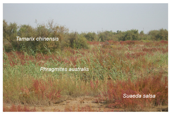
Figure 1.
Photo of community P.a, S.s, and T.c.
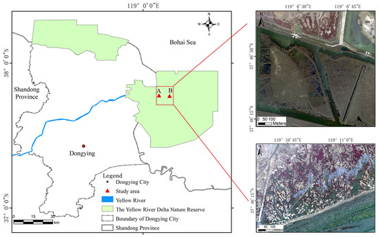
Figure 2.
The geographic location and aerial images of the study areas. The image in the upper right corner represents area A, and the image in the lower right corner represents area B.
2.2. Study Data
In this study, the image data of the YRD reservoir were obtained from the Cessna 208 B turboprop aircraft manufactured by CESSNA, Wichita, KS, USA, using a trilinear optical camera with a spatial resolution of 0.2 m. The sizes of the two images are 823 m × 611 m and 936 m × 900 m, respectively. And the acquisition time is in early October during the vegetation growth period. In this study, there are no strict requirements for the position and band range of the center wavelength of each band; therefore, the images obtained do not need to be strictly radiometrically calibrated. The images contained four bands: red (R), green (G), blue (B), and near-infrared (NIR). The coordinate system was WGS84, and the projection was the UTM. To unify the scale of the image data and eliminate dimensional differences between different features, the data of the four original bands were normalized.
2.3. Method
In this study, we used object-oriented classification methods based on color enhancement for fine classification of vegetation. The Technical flowchart is shown in Figure 3. First, we used the local variance of the ESP tool to determine the optimal segmentation scale, and second, the optimal shape factor and compactness factor were determined by experimental comparison. At the same time, color features are used to enhance the differentiation between different vegetation in the image. Based on multi-resolution segmentation, we use random forest (RF) [39], support vector machine (SVM) [40], k-nearest neighbor (KNN) [41] and maximum likelihood classifiers (MLC) [42] to classify the spectral features, texture features and vegetation features of the images. Color features are not only used as an auxiliary layer for object segmentation but also for optimal classification. Then, the confusion matrix calculation is used to evaluate the classification accuracy. Finally, the fine classification map of vegetation using the object-oriented classification based on color enhancement is visualized.
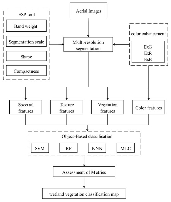
Figure 3.
Technical flowchart.
2.3.1. Image Color Characteristics
The color index is mainly used for 24-bit color images, and the red, green, and blue components of each pixel need to be calculated [43]. The R, G, and B channel data were divided by the maximum value of the image pixels for normalization. For 8-bit R, G, and B channels, the value is 255. Then, the color space is normalized to obtain the color components of the spectrum R, G, and B, and finally the color index is generated [44]. However, the color index can also be generated in other ways [45]; for example, for multispectral images, the value of the RGB color channel is changed depending on the hardware of the image acquisition camera, and some scholars directly use it to calculate the color index, but some studies have shown that an index using the normalized color channel may be more robust [46]. According to the interpretation signs, the color of the vegetation in the YRD has obvious differences. In the image, S.s is dark red, P.a is light yellow, and T.c is dark green. I.c does not stand out like these three typical vegetation types and appears bright green. The visible spectrum is normalized according to the method of processing 24-bit color images, and then the color space is normalized to obtain three color components to generate color features to improve the classification accuracy. The color space normalization formula is as follows:
In this study, the Excess green index (ExG) [47], Excess red index (ExR) [48] and Excess red index (ExB) [49] were used to strengthen the distinction of vegetation objects. The ExG, ExR, and ExB indices are commonly used as color features in vegetation analysis, agricultural remote sensing, or image processing, particularly in high-precision drone-based vegetation monitoring. Green vegetation strongly reflects green light, so ExG enhances the contrast between vegetation and backgrounds such as soil or bare land. ExR is sensitive to red objects and can effectively identify red salt marsh plants. ExB reflects strongly in water bodies, making it useful for distinguishing vegetation from other objects. They are calculated as follows:
ExG = 2g − r − b
ExR = 1.4r − g
ExB = 1.4b − g
2.3.2. Multi-Resolution Segmentation
Multi-resolution segmentation is based on object-oriented classification. Multi-resolution segmentation is used to generate homogeneous objects, which minimizes their average heterogeneity and maximizes their respective homogeneity, which is a necessary prerequisite for classification recognition and information extraction. This method allows for the continuous merging of pixels or objects and is a top-down segmentation based on the two-region merging technique. In the process of multi-resolution segmentation, there are four parameters that need to be set: band weight, segmentation scale, shape factor, and compactness.
In this paper, when segmenting the image, the weight value of all bands of the image is set to 1. First, four scales are used to set the split scale, and the rest are default values to determine the approximate range of the split scale. The experiment was carried out with 50 as the initial value and 50 as the step size, and the segmentation scales were 50, 100, 150 and 200, respectively. The segmentation effect is shown in Figure 4.
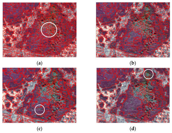
Figure 4.
Local segmentation results of different scales: (a) scale 50, (b) scale 100, (c) scale 150, (d) scale 200. The white circles are used to emphasize over-segmentation and under-segmentation areas.
The types of wetlands are complex, and the vegetation is unevenly distributed. This study mainly focuses on vegetation classification, so multi-resolution segmentation should take vegetation boundaries as an important reference. The white circles in the figure indicate the phenomenon of over-segmentation and under-segmentation. As can be seen from the figure, when the segmentation scale is 50, the segmentation is very fragmented, and the same type of feature is divided into multiple pieces. The whole segmentation effect is messy and blurry. When the scales are 150 and 200, the segmentation is incomplete, and the categories of objects are easily divided into one piece and merged into one object. When the scale is 100, the segmentation effect of various types of features is better. Therefore, 50–150 is used as a reasonable split range. The Estimation of Scale Parameter (ESP) tool based on the eCognition 8.9 software was used to assist in the selection of the optimal scale. The ESP tool works by calculating the mean of the local variance (LV) of different objects across multiple bands and, at the same time, measuring the rate of change (ROC) value of the LV [50]. The formula for calculating ROC is as follows:
where Ln is the local variance of the target layer and L(n−1) is the local variance of the next layer of the target layer. If the segmentation scale is larger than the target object, the correlation between most of the segmented objects will be greater, and the measurement of local variance will be lower. If the segmentation scale approximates the size of the target object, the variability between the objects increases and the local variance increases. In terms of the local variance on different segmentation scales, with the increase in the segmentation scale, the local variance will increase, until it matches the real features; then, the local variance will reach the maximum, and at this time the ROC reaches its maximum—that is, the optimal segmentation scale is obtained. ESP is not the only optimal scale, because the segmentation scale of vegetation is between 50 and 150, so after several trials we can find the optimal parameter.
First, the shape was selected as 0.1, and the compactness was 0.1, 0.3, 0.5, 0.7, and 0.9; the segmentation effect was the best when the compactness was 0.9. The compactness was determined to be 0.9, and the shape was set to 0.1, 0.3, 0.5, 0.7, and 0.9 for experimentation; the segmentation effect was found to be the best when the shape was 0.3. Therefore, the compactness was determined to be 0.9 and the shape factor was 0.3 after permutation and combination, as the segmentation effect was the best.
2.3.3. Vegetation Classification
In this study, the KNN, RF, SVM, and MLC were used for classification learning. All four are typical machine learning algorithms. Based on field surveys and visual interpretation, at least 150 sample points were randomly selected for each feature to evaluate the accuracy of the different classifiers. We will select the method with the highest accuracy to obtain the final vegetation map and assess the importance of its features.
Two sets of experiments were designed and each group of experiments was classified using four classifiers. The first set of experiments involved object-oriented classification, without using color features for segmentation optimization. The second group of experiments used object-oriented classification with color enhancement. In this way, we can verify the improvement effect of segmentation and classification optimized by color features and compare the advantages and disadvantages of different machine classifications to select the best classification method for future wetland vegetation classification mapping.
For both sets of experiments, we selected the exponential features listed in Table 1 for the classification. These include the spectral features, texture features, and vegetation index of the four original bands. Color features will not only be used to assist in the scale segmentation of the third set of experiments but will also be used to enhance the effect of color features. When using object-oriented classification, we calculate the mean and variance because an object contains multiple pixels.

Table 1.
The features used in all classifications.
In the texture analysis, five second-order statistics with small redundancy, namely, angular second moment (GLCM_A), correlation (GLCM_Cor), contrast (GLCM_Con), entropy (GLCM_E), and variance (GLCM_V), were selected for quantitative analysis of the images. The calculation methods are as follows:
In the above five equations, i represents the row, j represents the column, μi and μj represent the mean, σi and σj represent the variance, and P(i, j) represents the pixel value of the matrix (i, j). In order to avoid too many statistical components being generated during texture analysis of images, resulting in data redundancy and increasing the difficulty of calculation and extraction, the texture feature information was obtained after principal component analysis of the original image. Principal component analysis (PCA), also known as K-L Transform, is used in remote sensing images to calculate orthogonal linear transformations of features across multiple bands. Principal component analysis ensures that the mean square error is minimized and is often used to highlight certain features in remote sensing images. By transforming the four bands of the original image, principal component analysis concentrates the important information in the four bands in the first few principal components [51]. In the two study areas, the total contribution rates of the first two principal components were 96.83% and 98.68%, respectively. So the texture features were obtained by using these two principal components.
In order to enhance and distinguish between vegetation, water and bare land, four commonly used indices were applied to the vegetation index, namely the Normalized Difference Vegetation Index (NDVI) [52], Normalized Difference Water Index (NDWI) [28] and Soil Adjusted Vegetation Index (SAVI) [53]. The Equation is shown as follows:
2.3.4. Accuracy Evaluation Metrics
We used the OA, kappa coefficient, user precision, and producer precision to measure the accuracy and reliability of the results [35]. The OA and kappa coefficient represent the overall classification effect of the model. The user accuracy (UA) represents the probability that a pixel is classified into a given category that represents the real situation of the ground, and the producer accuracy (PA) represents the probability that the pixel is correctly classified.
3. Results
3.1. Image Segment Results
The segmentation of objects is a particularly important step in object classification, which is related to the accuracy of classification. Using the ESP tool, the optimal segmentation scale was determined to be 77, and the optimal scale was used to segment the study area. Because of the dark red S.s, light yellow P.a, dark green T.c and bright green I.c, the segmentation results can be optimized according to color features, and the types of vegetation can be better distinguished. The undivided area was refined to further divide the different targets, and the over-segmented targets were combined into the same object.
As shown in Figure 5, the object in (a) was too large, mixing P.a and T.c into one object. In (b), S.s was divided into two objects. However, optimized images (b) and (d) can effectively reduce the occurrence of this phenomenon. Because S.s is often a large area with a dense shape, the mixed phenomenon of P.a and T.c in the image is more obvious, and the distribution is relatively fragmented. Usually, the segmentation effect is based on the ability to distinguish the smallest shape of the ground. Therefore, S.s will still have over-segmentation.
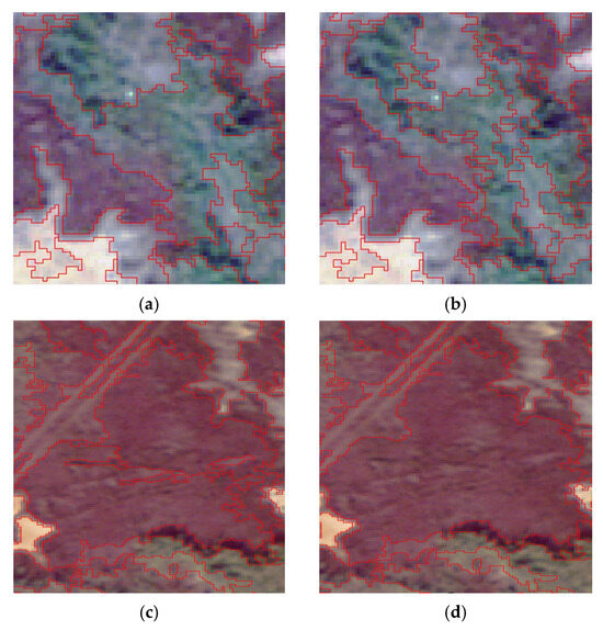
Figure 5.
Detailed comparison of vegetation segmentation before (a,c) and after (b,d) refinement of ill-segmented objects.
3.2. Results of Classification
Two sets of experiments were designed and each group of experiments was classified using four classifiers. The first set of experiments involved object-oriented classification, without using color features for segmentation optimization. The second set of experiments involved object-oriented classification with color features applied to refine classification accuracy through optimized color space transformation. In this way, we can verify the improvement effect of segmentation and classification optimized by color features and compare the advantages and disadvantages of different machine classifications to select the best classification method for future wetland vegetation classification mapping.
As shown in Table 2, RF and SVM can effectively extract each class of vegetation from 20 cm aerial images, with fewer misclassifications than MLC and KNN. RF achieved performance greater than 95% in both groups and was the optimal method. SVM follows closely behind, but in both groups, the UA for S.s and the PA for T.c are both below 90%, with some misclassifications and errors. MLC and KNN have lower accuracy, particularly in S.s and T.c. KNN had the lowest accuracy in both groups. Bare land, water, and I.c exhibit high PA and UA, maintaining stable accuracy across all methods in each group, indicating that these classes are relatively easy to distinguish. The classification results for I.c were particularly good, with PA and UA both exceeding 95%. Overall, these four classifiers are suitable for vegetation classification, with OA above 90% and Kappa greater than 0.9. RF and SVM have higher OA and Kappa than MLC and KNN, performing better in vegetation classification. Among them, RF has the highest OA and Kappa values, at 96.69% and 0.9603, respectively.
Table 2.
The comparison of classification accuracies.
The classification accuracy of the standardized confusion matrix is shown in Figure 6 to visually compare the classification results of the first and second groups. It can be found that after using color information, the accuracy of each method is improved to different degrees, and the misclassification is reduced to different degrees. The OA of the second group improved by 0.82–1.45% compared to that of the first group. The OA of RF improved the most by 1.45%, followed by MLC with an improvement of 1.25% and SVM with an improvement of 0.93%. The OA of KNN improved the least by 0.82%. In RF, using color information to optimize segmentation and classification reduced misclassification between the six classes (Figure 7). This was particularly evident in the misclassification between T.c and S.s. The misclassification of T.c as S.s decreased from 6.45% to 3.23%, while the misclassification of S.s as T.c decreased from 4.38% to 2.50%. This was a key factor in improving OA. The OA of SVM improved only slightly, by 0.93%, but it can be seen that misclassifications of S.s as P.a or bare land and misclassifications of T.c as S.s, have decreased. In MLC and KNN, the accuracies of the different classes exhibit different degrees of improvement. This indicates that this method can improve segmentation quality and classification accuracy. Ultimately, we chose to use the RF method optimized with color information for vegetation classification (Figure 8).
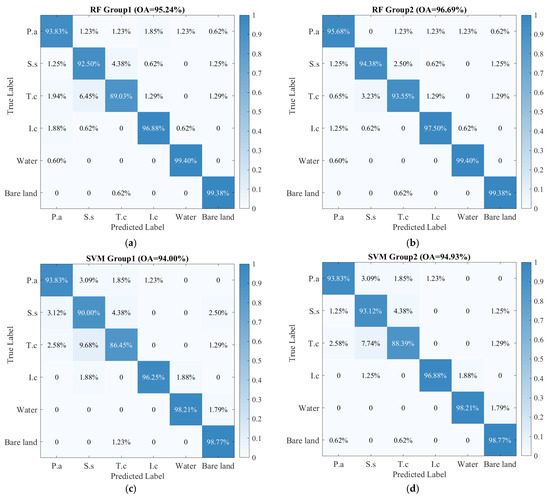
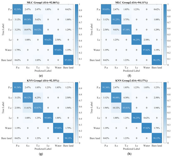
Figure 6.
Normalized confusion matrices of classification using RF (a,b), SVM (c,d), MLC (e,f), and KNN (g,h), in which (a,c,e,g) used color information. In contrast, (b,d,f,h) did not use color information.
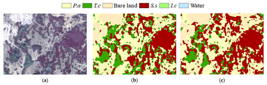
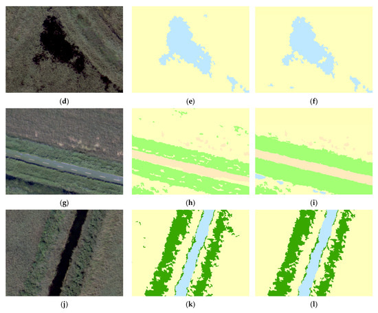
Figure 7.
The RGB true color composite imagery (a,d,g,j) in study areas. (b,e,h,k) did not use color information. In contrast, (c,f,i,l) use color information.
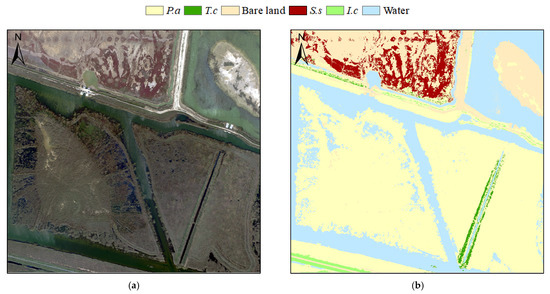
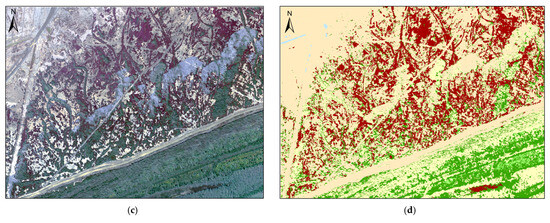
Figure 8.
The RGB true color composite imagery in study Area A (a) and study Area B (c) and distribution of vegetation in study Area A (b) and study Area B (d).
To quantify the importance of color features and other features in classification, we calculated feature importance. As shown in Figure 9, the red bars represent color features, the yellow bars represent the original band, the green bars represent vegetation features, and the gray bars represent texture features. Among them, three color features are in the top five. Feature ExB has an importance of 17% and ranks first, with ExB importance greater than the B band, ExG importance greater than the G band, and ExR importance greater than the R band. The ten texture features are at the bottom and all below 1.5%, indicating that texture features have a minor influence. This may also suggest that the boundaries of vegetation distribution are blurred, with no clear or fixed texture. Except for SAVI, which has a relatively low importance, the importance of other vegetation features and original bands is all greater than 5%, indicating that they also have some influence in classification. In summary, color features indeed play a significant role in extracting salt marsh vegetation in YRD, further validating that color features contribute to the improvement in OA.
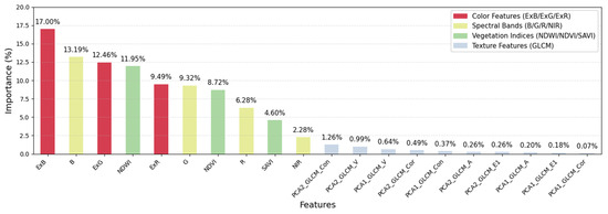
Figure 9.
The distribution of feature importance. PCA1_GLCM_V is the angular second moment of the first principal component, PCA2_GLCM_V is the angular second moment of the second principal component, and so on.
4. Discussion
A large number of studies have used remote sensing data to classify coastal vegetation. It is worth noting that most of these studies have used a spatial resolution of ten-meter or meter level [23,54,55,56]. Although this resolution allows for analysis of vegetation as a whole or at the level of vegetation communities, in-depth detection can promote understanding of land–vegetation coordination mechanisms. The importance of mapping coastal vegetation using high-resolution data has been emphasized in many studies that have used sub-meter spatial resolution to obtain location-specific characteristics and precise information on vegetation communities [57,58,59,60,61].
Pixel-based methods can lead to the “salt and pepper phenomenon”, which is mainly related to the misdetection of individuals within a community. Object-oriented methods can show distinct landscape patches. The most critical part of object-oriented classification is image segmentation. The segmentation results will directly affect the accuracy of vegetation classification. In image segmentation, the scale of segmentation determines the size of the segmentation object, which has a significant impact on the segmentation quality. The ESP tool calculates the rate of change of local variance through stepwise segmentation and automatically extracts three scale levels [62]. Shape and compactness are the other two factors that need to be set, which are the composition of the homogeneity criterion as implemented in the multi-resolution segmentation. The optimal values are also obtained through experimental comparison.
Many classifications are optimized by using temporal features or vegetation phenology features [23]. However, it is necessary to obtain multitemporal high-resolution aerial images, which are sometimes not available due to weather or short-term monitoring. Spectral features, temporal features, and texture features have been commonly used to classify coastal vegetation [13,61,63]. Although color features have been shown to be of great significance in fine agriculture, there is little literature discussing the role of color features in classifying wetland vegetation. The vegetation communities in the YRD exhibit distinct visual color differences, particularly the S.s, which is dark red. To compensate for the limitations of aerial imagery, which has few spectral bands and lacks long-term phenological characteristics, we incorporated color features of the YRD’s vegetation communities into image segmentation and classification features. This aims to enhance inter-class distinguishability under high-resolution aerial imagery and improve the distinguishability between vegetation and other classes, as well as among vegetation classes. Therefore, we used color features in both image segmentation and classification features.
In this study, color features are added to enhance segmentation, improve the accuracy of segmentation, and reduce over-segmentation and under-segmentation. However, the segmentation scale of each type of class in the study area is inconsistent, and this paper takes smaller features as the benchmark in the local area to make the classification more accurate. Therefore, S.s and bare land will still be over-segmented. For larger and more complex research areas, where there are abundant types of classes, a multi-level segmentation and classification system can be constructed according to different objects, so as to avoid a single scale affecting the classification efficiency and accuracy. At the same time, we believe that the method should theoretically be used in good weather with sufficient light. In cloudy weather or low light conditions, the color enhancement effect may be reduced but still effective. This is because the lack of light or environmental factors may cause the vegetation color to change, but it does not change the fact that the differences in color characteristics between vegetation classes still exist. It is more important to address the problem of large intra-class differences in the images obtained from uneven lighting, and it is best to perform a homogenization process before preprocessing.
The object features represent the relevant information of the objects and the spatial relationships between the objects. We calculate the mean and variance of each object’s features, and then we can distinguish different classes based on their differences. Spectral features, texture features, and vegetation features were integrated as classification feature sets, while color features were also involved in classification. Our study shows that RF outperforms SVM, KNN, and MLC in classification results, and this conclusion is consistent with many findings [64]. The basic unit of RF is the decision tree, and RF is essentially an ensemble learning of multiple decision trees. The number of decision trees involved in classification is consistent with the number of classification results, and the RF integrates all the classification results to determine the best sample class. Many results have proved that RF has high classification accuracy, fast efficiency and good stability [65]. Although SVM is also commonly used for classification, its effectiveness is slightly lower than that of RF. In two typical vegetation growth areas of salt marsh vegetation, KNN and MLC were not as good as RF and SVM in this classification result, but they could also effectively classify vegetation.
The classification model using color enhancement showed high accuracy in this study area, but the performance may be different in other wetland areas due to differences in image acquisition conditions, vegetation phenology and spectral characteristics. Although the results of the study indicate the potential of the color enhancement method in fine-scale wetland vegetation classification in the YRD, the study focused on the dominant communities in this area, which may vary due to differences in vegetation communities in other wetland areas. Therefore, wider validation could be carried out in multiple regions and ecological zones in the future.
Monitoring salt marsh vegetation in coastal wetlands is the basis of wetland research. In this study, aerial images of coastal wetlands in the YRD in Dongying City were taken as research objects. In this study, an object-oriented classification method based on color feature enhancement was proposed to classify wetland salt marsh vegetation. Spectral, texture, and vegetation features were used as inputs for the four machine learning classifiers. To verify the classification accuracy of the method, an object-based method without color feature enhancement was used to compare the classification results when the classifier was the same. We compared OA, kappa, PA, and UA of these methods. Based on the above studies, the following conclusions can be drawn:
(1) This study demonstrated the feasibility of using high-resolution aerial images for wetland vegetation classification. An object-oriented classification method based on color feature enhancement has also been explored.
(2) This study confirms that in the mixed areas and homogeneous zones of salt marsh vegetation, four machine learning methods can effectively classify vegetation according to the classification map and accuracy evaluation, among which the accuracy of SVM and RF is higher than that of MLC and KNN, and RF has the highest accuracy.
(3) In scale segmentation, color features are added to assist optimization and classification simultaneously, and the accuracy of the four classifiers is significantly improved. Owing to the large color difference in the image representation of wetland vegetation in the YRD, the addition of color features can better distinguish various types of vegetation, which is the key to distinguishing wetland vegetation in this study.
5. Conclusions
In this study, we proposed a method based on color enhancement to classify wet-land vegetation with 20 cm aerial imagery. We distinguished the mixed vegetation areas of salt marshes in the YRD of China and compared the classification accuracies of four classifiers: RF, SVM, KNN, and MLC. The results show that RF shows better accuracy in classification mapping, and it is also found that adding color features for segmentation and classification can better distinguish various types of classes in the YRD. To contribute to the conservation and restoration of vegetation, this study provides an effective method for fine classification of vegetation in the YRD from high-resolution aerial images.
Author Contributions
Conceptualization, Y.L. and Q.L.; methodology, Y.L.; software, Q.L.; validation, Y.Z.; formal analysis, Y.P.; investigation, C.C.; resources, X.Z.; data curation, Z.L.; writing—original draft preparation, Y.L. and Y.Z.; writing—review and editing, X.Z., Q.L., C.H. and H.L.; visualization, Y.L.; supervision, Q.L.; project administration, X.Z.; funding acquisition, Q.L. and X.Z. All authors have read and agreed to the published version of the manuscript.
Funding
This research was funded by the National Key Research and Development Program of China, grant number 2021YFB3901305; the Qilu Research Institute, grant number QLZB76-2023-000059; and the Key Laboratory of Natural Resource Coupling Process and Effects, grant number 2023KFKTB003.
Data Availability Statement
Data is unavailable due to privacy or ethical restrictions.
Conflicts of Interest
The authors declare no conflicts of interest.
References
- Guo, M.; Li, J.; Sheng, C.L.; Xu, J.W.; Wu, L. A Review of Wetland Remote Sensing. Sensors 2017, 17, 777. [Google Scholar] [CrossRef]
- Vehmaa, A.; Lanari, M.; Jutila, H.; Mussaari, M.; Pätsch, R.; Telenius, A.; Banta, G.; Eklöf, J.; Jensen, K.; Krause-Jensen, D.; et al. Harmonization of Nordic coastal marsh habitat classification benefits conservation and management. Ocean Coast. Manage 2024, 252, 107104. [Google Scholar] [CrossRef]
- Dutkiewicz, S.; Hickman, A.E.; Jahn, O.; Henson, S.; Beaulieu, C.; Monier, E. Ocean colour signature of climate change. Nat. Commun. 2019, 10, 578. [Google Scholar] [CrossRef] [PubMed]
- Nienhuis, J.H.; Ashton, A.D.; Edmonds, D.A.; Hoitink, A.J.F.; Kettner, A.J.; Rowland, J.C.; Tornqvist, T.E. Global-scale human impact on delta morphology has led to net land area gain. Nature 2020, 577, 514–518. [Google Scholar] [CrossRef]
- Wang, X.X.; Xiao, X.M.; Xu, X.; Zou, Z.H.; Chen, B.Q.; Qin, Y.W.; Zhang, X.; Dong, J.W.; Liu, D.Y.; Pan, L.H.; et al. Rebound in China’s coastal wetlands following conservation and restoration. Nat. Sustain. 2021, 4, 1076–1083. [Google Scholar] [CrossRef]
- Murray, N.J.; Phinn, S.R.; DeWitt, M.; Ferrari, R.; Johnston, R.; Lyons, M.B.; Clinton, N.; Thau, D.; Fuller, R.A. The global distribution and trajectory of tidal flats. Nature 2019, 565, 222–225. [Google Scholar] [CrossRef] [PubMed]
- Blum, M.D.; Roberts, H.H. Drowning of the Mississippi Delta due to insufficient sediment supply and global sea-level rise. Nat. Geosci. 2009, 2, 488–491. [Google Scholar] [CrossRef]
- Murray, N.J.; Clemens, R.S.; Phinn, S.R.; Possingham, H.P.; Fuller, R.A. Tracking the rapid loss of tidal wetlands in the Yellow Sea. Front. Ecol. Environ. 2014, 12, 267–272. [Google Scholar] [CrossRef]
- Gedan, K.B.; Silliman, B.R.; Bertness, M.D. Centuries of Human-Driven Change in Salt Marsh Ecosystems. Annu. Rev. Mar. Sci. 2009, 1, 117–141. [Google Scholar] [CrossRef]
- Syvitski, J.P.M.; Vörösmarty, C.J.; Kettner, A.J.; Green, P. Impact of humans on the flux of terrestrial sediment to the global coastal ocean. Science 2005, 308, 376–380. [Google Scholar] [CrossRef]
- Cui, B.S.; He, Q.; Gu, B.H.; Bai, J.H.; Liu, X.H. China’s Coastal Wetlands: Understanding Environmental Changes and Human Impacts for Management and Conservation. Wetlands 2016, 36, S1–S9. [Google Scholar] [CrossRef]
- He, X.H.; Hörmann, G.; Strehmel, A.; Guo, H.L.; Fohrer, N. Natural and Anthropogenic Causes of Vegetation Changes in Riparian Wetlands Along the Lower Reaches of the Yellow River, China. Wetlands 2015, 35, 391–399. [Google Scholar] [CrossRef]
- Deng, T.F.; Fu, B.L.; Liu, M.; He, H.C.; Fan, D.L.; Li, L.L.; Huang, L.K.; Gao, E.T. Comparison of multi-class and fusion of multiple single-class SegNet model for mapping karst wetland vegetation using UAV images. Sci. Rep. 2022, 12, 13270. [Google Scholar] [CrossRef] [PubMed]
- Nicholls, R.J. Coastal flooding and wetland loss in the 21st century: Changes under the SRES climate and socio-economic scenarios. Glob. Environ. Change 2004, 14, 69–86. [Google Scholar] [CrossRef]
- Jiang, C.; Chen, S.L.; Pan, S.Q.; Fan, Y.S.; Ji, H.Y. Geomorphic evolution of the Yellow River Delta: Quantification of basin scale natural and anthropogenic impacts. Catena 2018, 163, 361–377. [Google Scholar] [CrossRef]
- Li, H.; Liu, Q.S.; Huang, C.; Zhang, X.; Wang, S.X.; Wu, W.; Shi, L. Variation in Vegetation Composition and Structure across Mudflat Areas in the Yellow River Delta, China. Remote Sens. 2024, 16, 3495. [Google Scholar] [CrossRef]
- Mahdavi, S.; Salehi, B.; Granger, J.; Amani, M.; Brisco, B.; Huang, W.M. Remote sensing for wetland classification: A comprehensive review. Gisci. Remote Sens. 2018, 55, 623–658. [Google Scholar] [CrossRef]
- Wulder, M.A.; Roy, D.P.; Radeloff, V.C.; Loveland, T.R.; Anderson, M.C.; Johnson, D.M.; Healey, S.; Zhu, Z.; Scambos, T.A.; Pahlevan, N.; et al. Fifty years of Landsat science and impacts. Remote Sens. Environ. 2022, 280, 113195. [Google Scholar] [CrossRef]
- Sá, C.; Grieco, J. Open Data for Science, Policy, and the Public Good. Rev. Policy Res. 2016, 33, 526–543. [Google Scholar] [CrossRef]
- Zhu, W.Q.; Ren, G.B.; Wang, J.P.; Wang, J.B.; Hu, Y.B.; Lin, Z.Y.; Li, W.; Zhao, Y.J.; Li, S.B.; Wang, N. Monitoring the Invasive Plant in Jiangsu Coastal Wetland Using MRCNN and Long-Time Series Landsat Data. Remote Sens. 2022, 14, 2630. [Google Scholar] [CrossRef]
- Feng, K.D.; Mao, D.H.; Qiu, Z.Q.; Zhao, Y.X.; Wang, Z.M. Can time-series Sentinel images be used to properly identify wetland plant communities? Gisci. Remote Sens. 2022, 59, 2202–2216. [Google Scholar] [CrossRef]
- Ke, L.A.; Lu, Y.; Tan, Q.; Zhao, Y.; Wang, Q.M. Precise mapping of coastal wetlands using time-series remote sensing images and deep learning model. Front. Glob. Change 2024, 7, 1409985. [Google Scholar] [CrossRef]
- Li, H.Y.; Wan, J.H.; Liu, S.W.; Sheng, H.; Xu, M.M. Wetland Vegetation Classification through Multi-Dimensional Feature Time Series Remote Sensing Images Using Mahalanobis Distance-Based Dynamic Time Warping. Remote Sens. 2022, 14, 501. [Google Scholar] [CrossRef]
- Li, C.; Cui, H.W.; Tian, X.L. A Novel CA-RegNet Model for Macau Wetlands Auto Segmentation Based on GF-2 Remote Sensing Images. Appl. Sci. 2023, 13, 12178. [Google Scholar] [CrossRef]
- Liu, Q.S.; Huang, C.; Liu, G.H.; Yu, B.W. Comparison of CBERS-04, GF-1, and GF-2 Satellite Panchromatic Images for Mapping Quasi-Circular Vegetation Patches in the Yellow River Delta, China. Sensors 2018, 18, 2733. [Google Scholar] [CrossRef] [PubMed]
- Zweig, C.L.; Burgess, M.A.; Percival, H.F.; Kitchens, W.M. Use of Unmanned Aircraft Systems to Delineate Fine-Scale Wetland Vegetation Communities. Wetlands 2015, 35, 303–309. [Google Scholar] [CrossRef]
- González, E.; Sher, A.A.; Tabacchi, E.; Masip, A.; Poulin, M. Restoration of riparian vegetation: A global review of implementation and evaluation approaches in the international, peer-reviewed literature. J. Environ. Manag. 2015, 158, 85–94. [Google Scholar] [CrossRef]
- Fan, Y.S.; Yu, S.B.; Wang, J.H.; Li, P.; Chen, S.L.; Ji, H.Y.; Li, P.; Dou, S.T. Changes of Inundation Frequency in the Yellow River Delta and Its Response to Wetland Vegetation. Land 2022, 11, 1647. [Google Scholar] [CrossRef]
- Dronova, I.; Kislik, C.; Dinh, Z.; Kelly, M. A Review of Unoccupied Aerial Vehicle Use in Wetland Applications: Emerging Opportunities in Approach, Technology, and Data. Drones 2021, 5, 45. [Google Scholar] [CrossRef]
- Dronova, I. Object-Based Image Analysis in Wetland Research: A Review. Remote Sens. 2015, 7, 6380–6413. [Google Scholar] [CrossRef]
- Zheng, J.Y.; Hao, Y.Y.; Wang, Y.C.; Zhou, S.Q.; Wu, W.B.; Yuan, Q.; Gao, Y.; Guo, H.Q.; Cai, X.X.; Zhao, B. Coastal Wetland Vegetation Classification Using Pixel-Based, Object-Based and Deep Learning Methods Based on RGB-UAV. Land 2022, 11, 2039. [Google Scholar] [CrossRef]
- Zaabar, N.; Niculescu, S.; Kamel, M.M. Application of Convolutional Neural Networks With Object-Based Image Analysis for Land Cover and Land Use Mapping in Coastal Areas: A Case Study in Ain Temouchent, Algeria. IEEE J. Sel. Top. Appl. Earth Obs. Remote Sens. 2022, 15, 5177–5189. [Google Scholar] [CrossRef]
- Mahdianpari, M.; Salehi, B.; Rezaee, M.; Mohammadimanesh, F.; Zhang, Y. Very Deep Convolutional Neural Networks for Complex Land Cover Mapping Using Multispectral Remote Sensing Imagery. Remote Sens. 2018, 10, 1119. [Google Scholar] [CrossRef]
- Liu, T.; Abd-Elrahman, A.; Morton, J.; Wilhelm, V.L. Comparing fully convolutional networks, random forest, support vector machine, and patch-based deep convolutional neural networks for object-based wetland mapping using images from small unmanned aircraft system. Gisci. Remote Sens. 2018, 55, 243–264. [Google Scholar] [CrossRef]
- Zhang, C.; Gong, Z.N.; Qiu, H.C.; Zhang, Y.; Zhou, D.M. Mapping typical salt-marsh species in the Yellow River Delta wetland supported by temporal-spatial-spectral multidimensional features. Sci. Total Environ. 2021, 783, 147061. [Google Scholar] [CrossRef]
- Chang, D.; Wang, Z.Y.; Ning, X.G.; Li, Z.J.; Zhang, L.; Liu, X.T. Vegetation changes in Yellow River Delta wetlands from 2018 to 2020 using PIE-Engine and short time series Sentinel-2 images. Front. Mar. Sci. 2022, 9, 77050. [Google Scholar] [CrossRef]
- Wan, L.; Li, Y.J.; Cen, H.Y.; Zhu, J.P.; Yin, W.X.; Wu, W.K.; Zhu, H.Y.; Sun, D.W.; Zhou, W.J.; He, Y. Combining UAV-Based Vegetation Indices and Image Classification to Estimate Flower Number in Oilseed Rape. Remote Sens. 2018, 10, 1484. [Google Scholar] [CrossRef]
- Boutiche, Y.; Abdesselam, A.; Chetih, N.; Khorchef, M.; Ramou, N. Robust vegetation segmentation under field conditions using new adaptive weights for hybrid multichannel images based on the Chan-Vese model. Ecol. Inform. 2022, 72, 101850. [Google Scholar] [CrossRef]
- Ho, T.K. The random subspace method for constructing decision forests. IEEE Trans. Pattern Anal. Mach. Intell. 1998, 20, 832–844. [Google Scholar] [CrossRef]
- Cortes, C.; Vapnik, V. Support-Vector Networks. Mach. Learn. 1995, 20, 273–297. [Google Scholar] [CrossRef]
- Fix, E.; Hodges, J.L. Nonparametric Discrimination: Small-Sample Performance in Normal Populations. Ann. Math. Stat. 1951, 22, 487. [Google Scholar]
- Bruzzone, L.; Prieto, D.F. Unsupervised retraining of a maximum-likelihood classifier for the analysis of multitemporal remote-sensing images. In Proceedings of the SPIE Image and Signal Processing for Remote Sensing V, Florence, Italy, 20–24 September 1999; Volume 3871, pp. 169–174. [Google Scholar] [CrossRef]
- Hamuda, E.; Glavin, M.; Jones, E. A survey of image processing techniques for plant extraction and segmentation in the field. Comput. Electron. Agric. 2016, 125, 184–199. [Google Scholar] [CrossRef]
- Meyer, G.E.; Neto, J.C. Verification of color vegetation indices for automated crop imaging applications. Comput. Electron. Agric. 2008, 63, 282–293. [Google Scholar] [CrossRef]
- Mardanisamani, S.; Eramian, M. Segmentation of vegetation and microplots in aerial agriculture images: A survey. Plant Phenome J. 2022, 5, e20042. [Google Scholar] [CrossRef]
- Lee, M.K.; Golzarian, M.R.; Kim, I. A new color index for vegetation segmentation and classification. Precis. Agric. 2021, 22, 179–204. [Google Scholar] [CrossRef]
- Woebbecke, D.M.; Meyer, G.E.; Vonbargen, K.; Mortensen, D.A. Color Indexes for Weed Identification under Various Soil, Residue, and Lighting Conditions. Trans. Am. Soc. Agric. Biol. Eng. 1995, 38, 259–269. [Google Scholar] [CrossRef]
- Meyer, G.E.; Hindman, T.; Laksmi, K. Machine vision detection parameters for plant species identification. In Proceedings of the SPIE Precision Agriculture and Biological Quality, Boston, MA, USA, 1–6 November 1998; Volume 3543, pp. 327–335. [Google Scholar] [CrossRef]
- Guijarro, M.; Pajares, G.; Riomoros, I.; Herrera, P.J.; Burgos-Artizzu, X.P.; Ribeiro, A. Automatic segmentation of relevant textures in agricultural images. Comput. Electron. Agric. 2011, 75, 75–83. [Google Scholar] [CrossRef]
- Dragut, L.; Tiede, D.; Levick, S.R. ESP: A tool to estimate scale parameter for multiresolution image segmentation of remotely sensed data. Int. J. Geogr. Inf. Sci. 2010, 24, 859–871. [Google Scholar] [CrossRef]
- Li, Y.R.; Yu, X.; Zhang, J.H.; Zhang, S.C.; Wang, X.P.; Kong, D.L.; Yao, L.L.; Lu, H. Improved Classification of Coastal Wetlands in Yellow River Delta of China Using ResNet Combined with Feature-Preferred Bands Based on Attention Mechanism. Remote Sens. 2024, 16, 1860. [Google Scholar] [CrossRef]
- Ba, Q.; Wang, B.D.; Zhu, L.B.; Fu, Z.M.; Wu, X.; Wang, H.J.; Bi, N.S. Rapid change of vegetation cover in the Huanghe (Yellow River) mouth wetland and its biogeomorphological feedbacks. CATENA 2024, 238, 107875. [Google Scholar] [CrossRef]
- Huete, A.R. A Soil-Adjusted Vegetation Index (Savi). Remote Sens. Environ. 1988, 25, 295–309. [Google Scholar] [CrossRef]
- Peng, K.F.; Jiang, W.G.; Hou, P.; Wu, Z.F.; Ling, Z.Y.; Wang, X.Y.; Niu, Z.G.; Mao, D.H. Continental-scale wetland mapping: A novel algorithm for detailed wetland types classification based on time series Sentinel-1/2 images. Ecol. Indic. 2023, 148, 110113. [Google Scholar] [CrossRef]
- Han, Y.F.; Chi, H.; Huang, J.L.; Shi, X.M.; Qiu, J.; Shao, Q.H.; Li, Y.F.; Cheng, C.; Ling, F. Long-term wetland mapping at 10 m resolution using super-resolution and hierarchical classification—A case study in Jianghan Plain, China. Int. J. Digit. Earth 2025, 18, 2498605. [Google Scholar] [CrossRef]
- Liu, Q.S.; Huang, C.; Li, H. Mapping plant communities within quasi-circular vegetation patches using tasseled cap brightness, greenness, and topsoil grain size index derived from GF-1 imagery. Earth Sci. Inform. 2021, 14, 975–984. [Google Scholar] [CrossRef]
- Cruz, C.; O’Connell, J.; McGuinness, K.; Martin, J.R.; Perrin, P.M.; Connolly, J. Assessing the effectiveness of UAV data for accurate coastal dune habitat mapping. Eur. J. Remote Sens. 2023, 56, 2191870. [Google Scholar] [CrossRef]
- Zheng, B.; Shi, Y.S.; Wang, Q.; Zheng, J.W.; Lu, J. Fine Classification of Vegetation Under Complex Surface Cover Conditions with Hyperspectral and High-Spatial Resolution: A Case Study of the Xisha Area, Chongming District, Shanghai. J. Indian Soc. Remote Sens. 2025, 53, 1615–1626. [Google Scholar] [CrossRef]
- Bhatnagar, S.; Gill, L.; Regan, S.; Waldren, S.; Ghosh, B. A nested drone-satellite approach to monitoring the ecological conditions of wetlands. ISPRS J. Photogramm. Remote Sens. 2021, 174, 151–165. [Google Scholar] [CrossRef]
- Steenvoorden, J.; Bartholomeus, H.; Limpens, J. Less is more: Optimizing vegetation mapping in peatlands using unmanned aerial vehicles (UAVs). Int. J. Appl. Earth Obs. Geoinf. 2023, 117, 103220. [Google Scholar] [CrossRef]
- Fu, B.L.; Liu, M.; He, H.C.; Lan, F.W.; He, X.; Liu, L.L.; Huang, L.K.; Fan, D.L.; Zhao, M.; Jia, Z.L. Comparison of optimized object-based RF-DT algorithm and SegNet algorithm for classifying Karst wetland vegetation communities using ultra-high spatial resolution UAV data. Int. J. Appl. Earth Obs. Geoinf. 2021, 104, 102553. [Google Scholar] [CrossRef]
- Dragut, L.; Eisank, C. Automated object-based classification of topography from SRTM data. Geomorphology 2012, 141, 21–33. [Google Scholar] [CrossRef]
- Belcore, E.; Latella, M.; Piras, M.; Camporeale, C. Enhancing precision in coastal dunes vegetation mapping: Ultra-high resolution hierarchical classification at the individual plant level. Int. J. Remote Sens. 2024, 45, 4527–4552. [Google Scholar] [CrossRef]
- Sheykhmousa, M.; Mahdianpari, M.; Ghanbari, H.; Mohammadimanesh, F.; Ghamisi, P.; Homayouni, S. Support Vector Machine Versus Random Forest for Remote Sensing Image Classification: A Meta-Analysis and Systematic Review. IEEE J. Sel. Top. Appl. Earth Obs. Remote Sens. 2020, 13, 6308–6325. [Google Scholar] [CrossRef]
- Belgiu, M.; Dragut, L. Random forest in remote sensing: A review of applications and future directions. ISPRS J. Photogramm. Remote Sens. 2016, 114, 24–31. [Google Scholar] [CrossRef]
Disclaimer/Publisher’s Note: The statements, opinions and data contained in all publications are solely those of the individual author(s) and contributor(s) and not of MDPI and/or the editor(s). MDPI and/or the editor(s) disclaim responsibility for any injury to people or property resulting from any ideas, methods, instructions or products referred to in the content. |
© 2025 by the authors. Licensee MDPI, Basel, Switzerland. This article is an open access article distributed under the terms and conditions of the Creative Commons Attribution (CC BY) license (https://creativecommons.org/licenses/by/4.0/).