Article

Tree Type Classification from ALS Data: A Comparative Analysis of 1D, 2D, and 3D Representations Using ML and DL Models

1
Remote Sensing and Geoinformation, Institute for Digital Technologie, JOANNEUM RESEARCH Forschungsgesellschaft mbHs, 8010 Graz, Austria
2
Institute of Geodesy, Graz University of Technology, 8010 Graz, Austria
*
Author to whom correspondence should be addressed.
Remote Sens. 2025, 17(16), 2847; https://doi.org/10.3390/rs17162847
Submission received: 30 June 2025 / Revised: 8 August 2025 / Accepted: 11 August 2025 / Published: 15 August 2025
(This article belongs to the Section Forest Remote Sensing)

Abstract

Accurate classification of individual tree types is a key component in forest inventory, biodiversity monitoring, and ecological modeling. This study evaluates and compares multiple Machine Learning (ML) and Deep Learning (DL) approaches for tree type classification based on Airborne Laser Scanning (ALS) data. A mixed-species forest in southeastern Austria, Europe, served as the test site, with spruce, pine, and a grouped class of broadleaf species as target categories. To examine the impact of data representation, ALS point clouds were transformed into four distinct structures: 1D feature vectors, 2D raster profiles, 3D voxel grids, and unstructured 3D point clouds. A comprehensive dataset, combining field measurements and manually annotated aerial data, was used to train and validate 45 ML and DL models. Results show that DL models based on 3D point clouds achieved the highest overall accuracy (up to 88.1%), followed by multi-view 2D raster and voxel-based methods. Traditional ML models performed well on 1D data but struggled with high-dimensional inputs. Spruce trees were classified most reliably, while confusion between pine and broadleaf species remained challenging across methods. The study highlights the importance of selecting suitable data structures and model types for operational tree classification and outlines potential directions for improving accuracy through multimodal and temporal data fusion.

1. Introduction

Forests are essential ecosystems that provide a broad range of ecological, economic, and social functions. Globally, they represent the largest terrestrial biomass reservoir and are the second-most important carbon sink after the oceans. Beyond carbon storage, forests support biodiversity, regulate water cycles, offer recreational spaces, and supply renewable resources such as timber. Approximately two-thirds of all known terrestrial species (animals and plants) depend on forested habitats, making forests critical for global biodiversity conservation [1,2]. In light of climate change and increasing land-use pressure, the demand for accurate, large-scale, and repeatable forest monitoring continues to grow.
Modern forest inventories aim to quantify parameters such as forest structure [3,4], biomass [5], timber volume [6,7], species composition [8], and regeneration dynamics [9]. Historically, these tasks relied on extensive ground-based surveys [10], but such methods are time-consuming, labor-intensive, and spatially limited. Consequently, airborne remote sensing technologies, especially Airborne Laser Scanning (ALS), have emerged as indispensable tools for operational forest monitoring and ecological research [11,12].
ALS systems provide detailed 3D information on forest canopy structure by actively emitting laser pulses and recording their echoes. Unlike passive optical sensors, ALS systems are independent of illumination conditions and can operate in both leaf-on and leaf-off seasons. Advances in sensor technology now allow for multiple returns per pulse, full-waveform recording, and even multi-wavelength scanning, resulting in rich datasets capable of describing vertical vegetation profiles with high precision [13,14,15]. The integration of ALS with high-resolution aerial imagery, e.g., Red–Green–Blue (RGB), Near-Infrared (NIR) or hyperspectral, further enhances the potential for extracting biophysical forest parameters and classifying tree species at individual tree level [16,17].

1.1. Related Work

Individual Tree-Based Classification
This study employs a tree-based classification approach. Individual Tree Detection (ITD) and classification have become increasingly relevant for high-resolution forest analysis [4,18,19,20,21]. Unlike area-based approaches [22], ITD allows for species identification and parameter estimation at the level of single trees, enabling fine-grained forest modeling.
Numerous ITD methods have been proposed in the literature, broadly categorized into crown segmentation-based [23,24,25,26] and tree-top detection [27,28,29] approaches. In the first category, individual tree crowns are segmented first, from which the tree positions are then derived. In the second, the tree tops are detected directly. While classical rule-based methods still serve as baselines, Machine Learning (ML)- and Deep Learning (DL)-based approaches have shown improved robustness in complex forest conditions [30,31,32,33].
However, accurate tree classification following ITD remains challenging. The structural similarity between species can lead to classification ambiguity. Moreover, factors such as forest density, stand condition, crown overlap, acquisition conditions (e.g., leaf-on vs. leaf-off), and occlusion introduce significant variability into ALS data [34,35]. High point density (>5 pts/m2) has been identified as a prerequisite for reliable classification in structurally heterogeneous forests [36].
Features and Data Representations
Traditionally, tree classification from ALS data has relied on handcrafted features that describe geometric, radiometric, or waveform properties of the point cloud [37]. Geometric features, such as tree height percentiles (Hp), crown dimensions, point distribution metrics, and vertical structure indices, have been used to infer species-specific structural traits [4,38,39]. Radiometric features, including intensity statistics and echo ratios, provide information about surface reflectivity and have been shown to improve classification when combined with geometric descriptors [35,39,40,41].
Full-waveform Light Detection And Ranging (LiDAR) adds further classification potential by capturing the complete echo profile, enabling the extraction of metrics like waveform extent, number of peaks, and height of median energy [34,42,43,44]. While these features offer a more detailed characterization of tree structure, their extraction and interpretation require higher processing complexity.
More recently, data representations have moved beyond fixed descriptors toward holistic models that exploit the full structure of the tree crown. These include:
  • 1D feature vectors, summarizing handcrafted features derived from ALS data, including vertical (e.g., height percentiles), horizontal (e.g., crown width, base height), intensity-based, and structural distribution metrics [6,39].
  • 2D or 2.5D projections, such as rasterized crown profiles or canopy height maps [30,45,46].
  • 3D voxel grids, encoding local point densities [42].
  • 3D point cloud representations, which preserve the highest amount of structural detail [16,47].
1D feature vectors encode pre-defined structural summaries of individual trees, often categorized into geometric, radiometric, and waveform-based descriptors [37,38]. These handcrafted features are computationally efficient and interpretable, making them suitable for conventional ML models. Depending on the feature design, they can capture traits like crown asymmetry, base height, canopy density or signal return complexity, parameters that have shown relevance for species classification [18,48]. However, by compressing complex 3D crown architecture into summary statistics, such representations risk losing species-specific structural nuances, especially in morphologically similar taxa.
2D projections (e.g., Canopy Height Models, CHMs) rasterize the 3D point cloud into structured grids, allowing compatibility with standard Convolutional Neural Networks (CNN) architectures [22,30,49]. These representations are computationally efficient and work well for large-scale applications using image-based deep learning. However, rasterization results in the loss of volumetric context and internal crown detail, which limits their effectiveness in complex, multilayered canopies. As shown in multiple studies, important features like point distribution within the crown or penetration depth, crucial for species differentiation, are not well preserved in 2D formats [37]. Depending on the projection type (e.g., vertical profiles or horizontal slices), 2D representations may retain some structural aspects, but they still offer only a partial view of the canopy’s 3D architecture [22,30,45].
3D representations, such as voxel grids or unstructured point clouds, preserve the full spatial structure of trees (within the level of structural detail that ALS data can realistically capture) and offer more comprehensive information than lower-dimensional formats, enabling analysis of both external crown shape and internal vertical distribution. Voxel-based methods allow regular input for 3D CNNs but may smooth fine details and require dense point clouds for reliable results [42]. 3D point cloud-based models like PointNet++ [50] and PointCNN [51] operate directly on unstructured data and maintain high fidelity, especially in species with subtle structural differences [47,52]. However, these methods require high-quality training data and are computationally demanding.
Thus, dimensionality imposes a clear trade-off: 1D features are efficient but reductive, 2D projections are CNN-compatible but lossy, and 3D representations preserve structure but at higher computational cost. Selection of representation should therefore consider data availability, forest complexity, and operational constraints.
Machine Learning and Deep Learning Approaches
Various ML techniques have been employed for tree species classification using ALS-derived features. Algorithms such as Random Forest (RF), Support Vector Machines (SVM), k-Nearest Neighbors (k-NN), and Linear Discriminant Analysis (LDA) have shown reasonable performance when sufficient and well-designed features are available [13,18,53,54,55,56,57]. These methods require manual feature engineering and tend to plateau in performance when confronted with structurally similar species or noisy data.
In contrast, DL methods, especially CNNs and transformer-based models, allow for end-to-end learning of feature hierarchies from raw or minimally processed data. DL architectures have achieved outstanding results in image classification and are increasingly adapted for remote sensing applications, including tree detection and classification [30,31,45,46,47].
Early adaptations used Canopy Height Model (CHM) and normalized Digital Surface Model (nDSM) as CNN input, treating tree classification as a 2D image classification problem [22,30,45,46]. More advanced approaches, such as PointCNN [51] and Point Transformer [58], directly process unordered point clouds without requiring rasterization or voxelization, enabling end-to-end learning for tree species classification [47]. These methods preserve 3D structural information and have demonstrated higher classification accuracy, particularly in mixed and multilayered forests.
Yet, DL methods also pose practical challenges: they require large, annotated training datasets, are computationally intensive, and often lack interpretability. Especially in forestry contexts, where labeled data are limited and domain knowledge is essential, these factors constrain their operational use.

1.2. Research Gap and Contribution

Despite the considerable progress in tree species classification using ALS data, key methodological challenges remain, particularly regarding the impact of data representation on classification performance and generalizability. Existing studies often focus on specific model types or handcrafted features, but lack a systematic evaluation across different input structures. As a result, there is limited understanding of how model complexity, data preprocessing effort, and classification accuracy interact across varying representation strategies.
This study addresses this gap by conducting a comprehensive comparison of classification approaches based solely on geometric information from ALS data: 1D feature vectors, 2D rasterized images, 3D voxel grids, and 3D point cloud-based representations. Intensity was deliberately excluded in order to isolate the contribution of geometric structure alone. In doing so, it highlights trade-offs between feature engineering requirements and classification accuracy. The results offer practical guidance for the design of ALS-based classification workflows and contribute to the development of scalable, operationally feasible approaches for high-resolution forest monitoring. The presented findings are a focused selection from a broader research project carried out within the scope of the first author’s doctoral work.

1.3. Outline

After a short introduction to the topic and objectives of this study, the remainder of this paper is organized as follows: Section 2 introduces the study site, the available ALS and aerial image data, and the procedures used to collect training data. Section 3 describes the methods, including the preprocessing steps and classification approaches using four different data representations: 1D feature vectors, 2D raster data, 3D voxel data, and 3D point clouds. Section 4 presents the results, including validation methods and both quantitative and illustrative outcomes. Section 5 discusses the findings in terms of model behavior, reliability, and performance improvements, and provides implications for future applications. Section 6 concludes the paper and outlines potential future directions.

2. Materials

2.1. Study Site

Location and Geographical Description: The study site is situated in southeastern Austria, within the state of Styria, near Burgau (see Figure 1). It spans an elevation range from 260 to 370 m above sea level. The landscape is distinguished by its gentle hills, vineyards, and expansive forests. Notably, the area once contained several fishing ponds, which have since been largely overtaken by forest [59].
Fauna: The forests are crisscrossed with numerous hiking trails and serve as a habitat for a diverse range of plant and animal species. The study site is approximately 2 km wide and 8 km long, hosting various tree species. Predominant species include spruce, pine, larch, birch, beech, oak, ash and alder. This rich mix makes the area particularly challenging for individual tree detection and classification. Tree composition varies significantly based on soil conditions and moisture levels. Along creeks and former ponds, ash and alder trees are prevalent, while drier areas are dominated by a combination of spruce, pine, and oak [59]. The forest is largely a naturally regrow area but has been subject to partial management.
Climate: The regional climate is temperate, characterized by warm summers and relatively mild winters. This climatic condition contributes to the area’s diverse biological composition.

2.2. Data

Extensive research activities in the region have led to the availability of various datasets, including satellite and aerial imagery, ALS data, and field-based measurements. For this study, aerial images and ALS data are of particular relevance and will be described in the following subsections.

2.2.1. ALS Data

The ALS dataset used in this study was acquired on 1 September 2016, during a leaf-on condition in late summer. The survey was conducted using an ultralight aircraft flying at approximately 800 m above ground level. A RIEGL VQ-580 laser scanner (RIEGL, Horn, Austria) was employed, operating at a wavelength of 1064 nm, and capable of recording up to six echoes per laser pulse. This capability was particularly beneficial for capturing vertical vegetation structure in multi-layered forests.
The average point density of the dataset was approximately 16 points per square meter, providing a detailed representation of the forest canopy and upper structural layers.
The scan pattern was slightly forward-slanted, resulting in a uniform point distribution both along the flight direction and across-track. A total of eight flight strips, six in longitudinal and two in transverse direction, were recorded, with relatively strong overlap (estimated between 50% and 70%), ensuring sufficient point coverage and minimizing occlusion effects in dense or complex canopy structures.
Direct georeferencing was performed using a NovAtel SPAN-FSAS GPS/IMU system (Hexagon, Stockholm, Sweden), providing precise positioning and orientation of the sensor platform. In addition to ALS data, co-registered RGB and NIR aerial imagery was collected during the same flight campaign and is described in detail in the following section.

2.2.2. Aerial Images

The utilization of aerial images alongside ALS datasets significantly enhanced the comprehensiveness of the analysis. While the ALS data were directly used for classification, the aerial images were not used for automated classification but supported the collection of ground truth data and offered a broader perspective on forest structure and species composition. This was complemented by the high-resolution nature of the images, which allowed for detailed observations of individual tree groups or trees. The true orthophotos were generated from stereo images using Agisoft MetaShape software Version 1.2.5 (https://www.agisoft.com, accessed on 30 June 2025) as part of the photogrammetric processing workflow. Georeferencing was performed based on tie points derived from the ALS datasets. During the generation of true orthophotos, a deliberate emphasis was placed on achieving the highest possible geometric resolution. This approach occasionally resulted in minor artifacts in areas with significant height variations, such as the transition from ground level to the canopy at the edges of tall trees. However, this trade-off was deemed acceptable to obtain enhanced resolution of the tree crowns, thereby facilitating a more detailed structural analysis.
The study employed two distinct sets of aerial images, each contributing uniquely to the overall analysis:
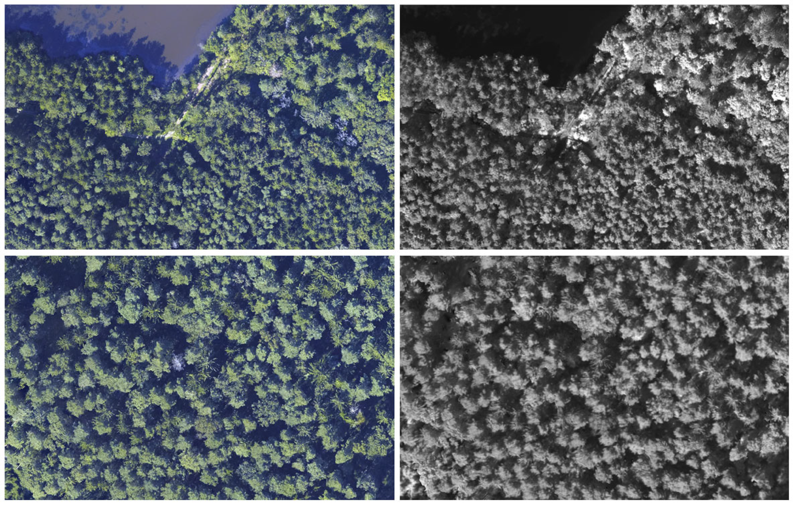
RGB Aerial Images (2016): These images, taken alongside with the ALS 2016 data, were processed in various resolutions (50, 25, 15 and 9 cm). The 9 cm resolution images were especially significant for deriving detailed information about tree crown structures and species. Two small examples are visualized in Figure 2 left.
NIR Aerial Images (2016): The Near-Infrared (NIR) Aerial Images were processed to match the 9 cm geometric resolution characteristic of the RGB true orthophotos. The NIR images, shown in Figure 2 right, were important in expanding the spectral data pool. The enrichment of spectral information from the NIR dataset—in combination with the RGB imagery—played a fundamental role in the manual acquisition of “ground truth” data on the computer (collection process is described in next sections). This aspect was particularly relevant in instances where the identification of tree species/types was ambiguous or unclear in other datasets, such as ALS or RGB. The enhanced spectral differentiation capabilities of the NIR imagery significantly facilitated the classification and distinction of various tree species/types, thereby improving the overall accuracy (OA) and reliability of ground truth data collection.

2.3. Training Data Collection

To train and evaluate the supervised classification models, two complementary strategies for reference data collection were employed: field-based surveys and manual annotation using ALS and high-resolution aerial imagery. These two approaches were chosen to balance data precision and dataset size. While field data provide highly accurate, ground-verified information, they are limited in quantity due to the resource-intensive nature of collection. In contrast, ALS and imagery data allow for the efficient labeling of a much larger number of samples across wider spatial extents, albeit with less direct ground truth. The combination of both sources was essential to generate a robust dataset that fulfills the high quantity and variability requirements of DL models.
While no formal consistency analysis was conducted between field-collected and manually annotated samples, both data sources were used exclusively to label dominant, co-dominant, and intermediate trees that are clearly visible in ALS and aerial imagery. For this specific task, species classification at the crown level, annotation consistency is considered high when performed by trained analysts, and species-level agreement between both sources is expected to be reliable. Most differences between the sources relate to the localization and detectability of suppressed trees, which are often not visible in ALS or aerial imagery and were excluded from manual annotation. However, these discrepancies are relevant mainly in stem mapping or completeness evaluations and do not affect the classification task addressed in this study.
The tree species considered in this study were grouped into three main classes for classification purposes: spruce, pine, and a third class referred to as broadleaf, which includes multiple broadleaf species such as beech, birch, oak, ash, and alder. Throughout this study, these three species groups are collectively referred to as tree types.
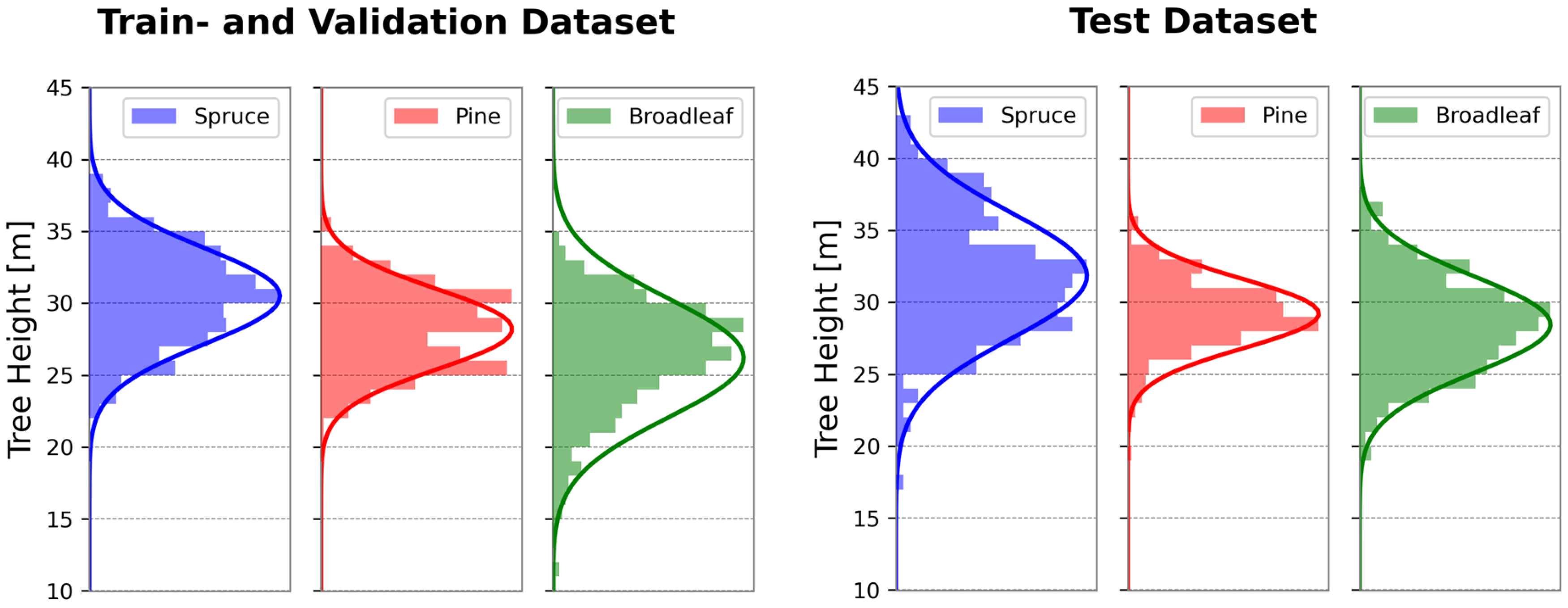
The final reference dataset integrates both field-collected and remotely derived samples and includes only trees from the dominant, co-dominant, and intermediate canopy layers, which are clearly visible in ALS and aerial imagery. Figure 3 illustrates the resulting tree height distributions for spruce, pine, and broadleaf classes, separately for the training/validation and independent test datasets. The class-specific height distribution across the datasets was consistent and reflected the study’s focus on upper canopy trees. Most trees were between 20 and 40 m tall, with a peak around 30 m. This dominance-oriented sampling directly influences how the models behave in application and is considered in later analysis.
The following subsections describe the data acquisition and processing methods in detail.

2.3.1. Ground Truth Data Collection in the Field

Field data collection was conducted across ten circular sample plots, each ranging in diameter from 25 to 55 m and distributed throughout the study area. Within these plots, data were gathered on tree location, height, species, and dominance. While only location and species are strictly necessary for classification tasks, additional parameters were also recorded and will be further discussed in subsequent sections.
Trees were included in the sample if they exceeded 7 m in height and had a Diameter at Breast Height (DBH) greater than 8 cm. The location of each tree was determined at approximately 1.3 m above ground level, using a combination of Leica Global Positioning System (GPS) and a total station system.
To ensure accurate and consistent data collection, a structured and reliable workflow was implemented. Each tree within a plot was assigned a unique Identifier (ID) (see Figure 4). These IDs were affixed to the trees facing the direction of the total station, allowing for pre-determination of the total number of trees to be recorded (i.e., based on the last ID used).
Tree locations were digitally recorded via the total station, while all attributes and metadata were documented in specially prepared field tables. After all trees were measured and documented, the ID tags were removed and checked for completeness. This method proved to be both efficient and reliable, incorporating automated verification steps to minimize errors or omissions.
Since the apex of a tree often does not align vertically with the measured stem location, a correction was needed to better align field data with ALS-visible tree top. Literature indicates that the horizontal offset between stem and apex varies significantly among species, on average 0.88 m for conifers and 1.54 m for broadleaf trees [60]. In some cases, such as oak and beech trees, the offset can reach up to 2.2–2.7 m [61]. The direction of this deviation is highly variable and influenced by local factors such as light competition and topography, making standardization impossible. Therefore, a manual correction was performed to adjust stem locations to the corresponding tree tops for alignment with ALS data. This correction was only feasible for dominant, co-dominant, and intermediate trees, which are visible in ALS and aerial imagery data. Suppressed trees, being smaller and typically obscured by canopy layers, were poorly or not visible in ALS data and thus excluded from correction, especially since they were not the focus of this study.
Tree height was measured using the Vertex IV system (https://haglofsweden.com/project/vertex-5, accessed on 30 June 2025). Before measurement, the device was acclimatized and calibrated. Calibration involved aligning a measuring tape on a flat surface (e.g., a road) to a fixed length (e.g., 10 m), placing the device at 0 m and the transponder at the end point. Calibration was triggered and completed within seconds, indicated by an auditory signal. Because temperature changes can affect the accuracy, calibration was repeated several times throughout the day to reduce potential errors.
Tree species were recorded in the field and categorized into ten groups: spruce, pine, oak, birch, larch, alder, maple, ash, beech, and “other”, the latter including rare broadleaf species grouped due to their low occurrence.
Tree dominance was also recorded (dominant, co-dominant, intermediate, and suppressed) to help identify suppressed trees, which are not visible in ALS or aerial imagery.
Diameter at Breast Height (DBH) was also recorded during fieldwork; however, this parameter was not used for classification in the present study.
In total, 793 trees across 10 species classes were recorded in the field. However, this dataset was insufficient for training DL models, which require significantly more data than traditional ML methods (e.g., RF, k-NN). The amount of data required for DL depends on factors such as model architecture, task complexity, data variability, class balance, and quality. Techniques like data augmentation [62] can help optimize performance when working with limited data, but their effect is restricted when the base dataset is very small. Approximately one-third of the field-collected trees were suppressed and not visible in ALS imagery; thus, they were excluded. Furthermore, the dataset showed imbalances between species classes. Given the high costs of field data collection, it was necessary to explore alternative, more resource-efficient strategies, such as deriving reference data from aerial imagery and ALS data.

2.3.2. Collection of Data from Aerial Imagery and ALS Data

To supplement the limited field data, additional training data were generated manually using existing ALS data and high-resolution RGB and NIR/CIR aerial imagery with a ground resolution of 9 cm. These sources enabled the identification and labeling of additional reference trees directly on-screen. Using this method, a set of automatically detected tree tops was manually assigned to one of three classes: spruce, pine, and broadleaf trees.
This on-screen generated dataset, combined with the field-collected data, consisted of 500 trees per class and was split into an 80/20% training/validation ratio. An independent test dataset of 261 trees per class was separately prepared and not used during training or hyperparameter tuning. This test set was specifically designed for objective evaluation:
  • About a quarter of the trees originated from the same area as the training data;
  • Another quarter came from nearby forests with similar structural and species characteristics;
  • The remaining half came from adjacent forests that differed in density, species mixture, and crown structure of broadleaf trees.
Together, the field-collected and aerial/ALS-derived datasets provided a robust foundation for the supervised classification tasks undertaken in this study. Figure 3 illustrates the distribution of tree heights across the compiled datasets.

3. Methods

The accurate classification of tree types based on ALS data requires a carefully designed processing and analysis pipeline. This study explores and compares four fundamentally different data representation approaches—1D vector-based, 2D raster-based, 3D voxel-based, and 3D point cloud-based methods—each offering distinct advantages and limitations in terms of data structure, feature extraction, and computational efficiency.
A central motivation for this multi-representational approach is the question of how much structural and semantic information is preserved, or potentially lost, when transforming the raw 3D point cloud into lower-dimensional forms. The ability to retain meaningful spatial patterns is particularly critical in tree type classification, where structural traits such as crown shape, branching, and height distribution play a key role. By systematically evaluating these representations, the study aims to identify the most effective and efficient format for maintaining classification accuracy.
Beyond information preservation, the use of 2D representations is motivated by the proven efficiency of CNNs in image analysis. Along with transformer-based vision models, CNNs benefit from standardized, dense input formats such as raster images. These models are well-established, hardware-optimized, and supported by a wide range of architectures and training strategies. Meanwhile, 3D voxel and point cloud-based models allow for the direct processing of spatial relationships in their native form, at the cost of increased complexity and computational demand. 1D vector-based methods, on the other hand, offer a compact and interpretable representation derived from handcrafted or semi-automated feature extraction processes.
This chapter outlines the entire classification pipeline, beginning with the general pre-processing of the ALS point cloud data (Section 3.1), followed by detailed descriptions of the methods used for each representation: 1D vector-based (Section 3.2), 2D raster-based (Section 3.3), 3D voxel-based (Section 3.4), and 3D point cloud-based approaches (Section 3.5).

3.1. Pre-Processing and Preparation of Data for ML- and DL-Based Tree Type Classification

Before applying the classification methods presented in the following sections (1D, 2D, and 3D approaches), the ALS point cloud data had to be carefully pre-processed through a series of custom tailored steps (see Figure 5). The processing begins with the raw ALS point cloud, from which an nDSM is derived. This forms the basis for further steps such as segmentation, filtering, and the derivation of features tailored to different data representations (e.g., 1D vectors, 2D rasters, 3D voxels, and point clouds; see Section 3.2.1, Section 3.3.1 and Section 3.4.1) that are suitable for ML and DL techniques. Each of these steps is described in more detail in the following subsections, with a focus on how they support the respective classification approaches.

3.1.1. Individual Tree Detection (ITD)

Since the classification is performed at the individual tree level, a reliable ITD process is required as a first step. Several of the ITD methods discussed in Section 1.1 were tested in this study and automatically compared [63,64]. The evaluation revealed that none of the methods were able to accurately detect all trees in the middle and upper canopy layers. Some trees were entirely missed, while others were detected multiple times. This observation aligns with findings from previous literature, which report varying detection accuracies depending not only on the algorithm but also on factors such as ALS point density, tree height, tree species, forest structure (single- or multi-layered), and forest type (e.g., mixed or coniferous) [64,65].
Since the subsequent classification relies on the output of the ITD process, it was crucial to ensure that all relevant trees were captured. To achieve a comprehensive detection of middle- and upper-layer trees, the parameters of the ITD methods (e.g., minimum crown size, smoothing radius) were adjusted to maximize the number of correctly identified tree crowns. As a result, some trees, especially broadleaf trees, were detected more than once. This can occur because broadleaf crowns often lack a clear apex, unlike conifers with a distinct peak. The algorithm may then interpret multiple local maxima within a single crown as separate trees. However, this was considered acceptable, as capturing all trees was prioritized. In cases of multiple detections, the affected trees were classified repeatedly. Importantly, results showed that such trees were mostly assigned the same class across all detections. Therefore, duplicate detections are less critical in this context than they would be, e.g., in applications requiring an exact tree count.

3.1.2. Extraction of Tree Crown

As mentioned previously, some ITD methods directly provide crown segments, which could in principle be used for further processing. However, tree crown segmentation is a non-trivial task, and numerous methods have been proposed in the literature [7,31,66,67,68,69,70,71]. Each of these methods introduces specific segmentation errors, which may negatively affect the subsequent classification. To avoid such compounding inaccuracies, this study deliberately refrains from using automated crown segmentation and instead adopts a simplified, geometry-based approach: a fixed-radius cylindrical extraction.
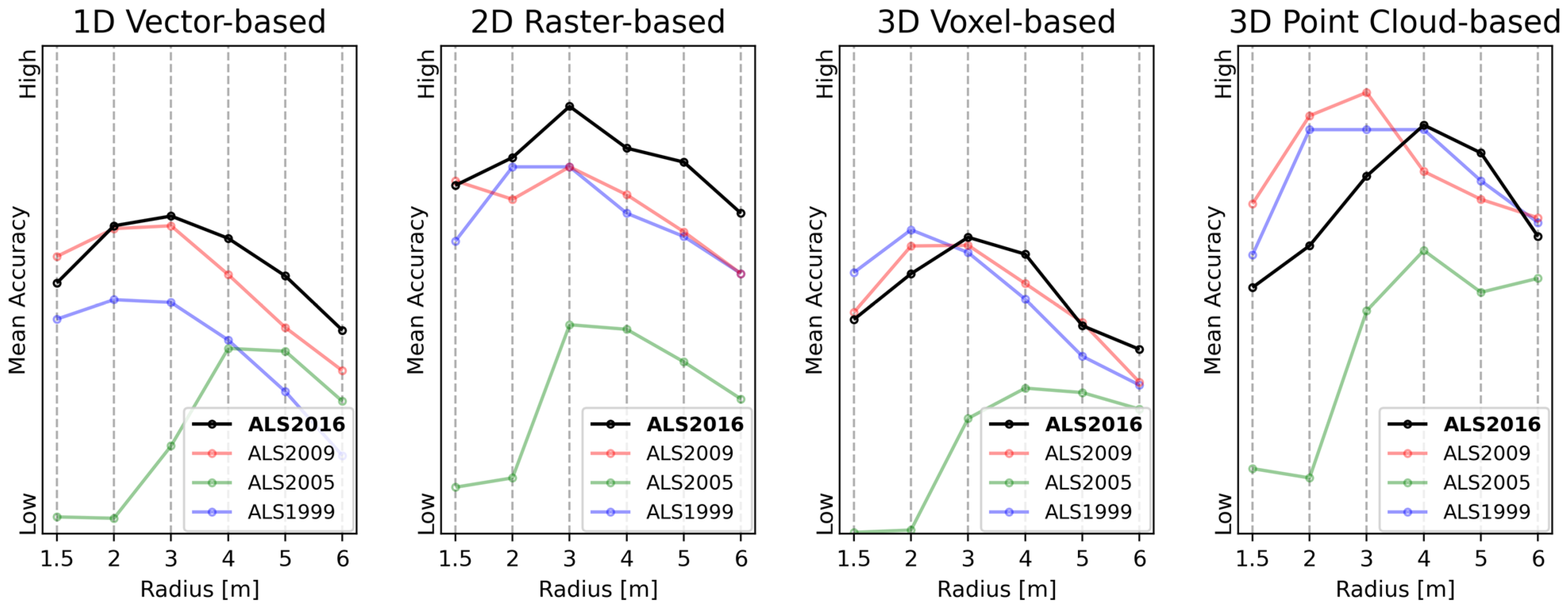
In this method, a cylinder with a predefined radius (R) is centered on each automatically detected tree top to define the spatial extent of the tree segment for classification (see Figure 5, lower right). The assumption behind this approach is that the neural network will learn to focus on the most relevant areas within the cylinder. This method ensures a uniform and consistent input structure across all trees. While small crowns may include data from neighboring trees and large crowns may not be fully captured, the central question in this context is how to determine the optimal radius. If the radius is too small, the model may lack sufficient information for accurate classification. If it is too large, data from neighboring trees may dominate, leading to classification errors. To identify a suitable balance, multiple radii (1.5, 2.0, 3.0, 4.0, 5.0, and 6.0 m) were empirically tested.
Although the main classification experiments in this study were conducted using the ALS dataset from 2016 (see Section 2.2.1), additional ALS datasets from 1999, 2005, and 2009 were included specifically for the analysis of the optimal crown extraction radius. These supplementary datasets vary in terms of point density and acquisition conditions, providing a broader empirical basis for evaluating the segmentation radius. This multi-temporal analysis ensures that the chosen radius of 3 m is not biased toward a single dataset, but instead reflects a robust and generalizable choice suitable for different ALS conditions.
As illustrated in Figure 6, a radius of 3 m produced the highest classification accuracies in most cases (except for ALS2005 dataset, which had a very low point density of only 2 points/m2) and showed the best average performance overall across all four data representations: 1D vector-based, 2D raster-based, 3D voxel-based, and 3D point cloud-based. This comparison allows for an evaluation of the influence of extraction radius across varying data structures and ALS data (in our case, four different acquisition years). The depicted values reflect mean accuracies across different algorithmic approaches in an early exploratory phase, in which no hyperparameter tuning was applied due to the high computational effort required for optimizing each model individually. The goal of this analysis is not the comparison of absolute accuracies (hence no numerical values on the Y-axis), but rather the identification of a robust radius value with stable performance across datasets. For all four data types, the results show a consistent trend: very small radii lack sufficient information, while large radii increasingly include neighboring tree data—both leading to reduced classification accuracy.
While combinations of multiple radii were also tested to potentially enhance model performance, these yielded either marginal or no improvements in accuracy. Moreover, they significantly increased computational complexity. For this reason, a single-radius approach was preferred.
By applying this cylinder-based crown extraction method with a fixed 3 m radius, a strong and consistent foundation for all further tree type classification tasks was established.

3.1.3. Computation of Normals and Curvature

For some classification approaches, the calculation of point cloud normals and curvature was included as part of the pre-processing pipeline. These geometric features capture local surface orientation and shape characteristics, which can reflect internal crown structure, branch orientation, and overall canopy complexity, information that can improve the differentiation between tree types.
These geometric descriptors were computed based on the nearest eight neighboring points. The choice of this number was empirically determined through ALS data analysis. Specifically, different neighborhood sizes were evaluated by examining both total and maximum distances between points within local neighborhoods. This process allowed for the identification of a median neighborhood size that likely captured only truly adjacent points—such as those belonging to the same tree branch—while excluding more distant points from neighboring trees. Although this method cannot guarantee perfect separation in all cases, it ensures that, for the majority of points, the computed normals and curvature values reflect local tree structure accurately and consistently.

3.1.4. Normalization of Data

In the next pre-processing step, all extracted crown segments were normalized, serving several important purposes. Most notably, normalization ensured that absolute tree height did not bias the classification process. Each tree segment was therefore scaled to a range of [−1, +1]. This range was chosen instead of [0, +1] to better suit the requirements of most neural networks, which tend to perform more reliably and accurately with inputs centered around zero.
To further enhance the generalization capability of the models, random scaling augmentation [62] was applied during normalization. This technique introduced variability by randomly adjusting the scale of tree segments by up to ±10% along the X, Y, and Z axes, increasing the diversity of the training data.
Figure 7 presents the normalized point distribution for reference data across the three tree types: spruce, pine, and broadleaf. To improve interpretability, all labeled reference segments (see Section 2.3) were aggregated by tree class before computing the vertical distribution, allowing consistent visualization of general structural differences. The x-axis reflects normalized point density, not absolute point counts or physical units, and is intended to illustrate the typical vertical distribution pattern of ALS returns across tree types. The y-axis shows normalized tree height, ranging from −1 (Ground) to +1 (Tree Top). The graph reveals class-specific differences in the vertical distribution of ALS returns, particularly concentrated in the upper third of the crowns. This pattern reflects the nature of Airborne Laser Scanning, where most laser pulses are returned from the upper canopy layers, with fewer reaching deeper crown regions. The insights gained from this distribution are fundamental for feature extraction. For example, the ratios of vertical point density can serve as powerful features for classification. In Figure 7 (right side), vertical layer 11 contains notably more points in spruce compared to pine and broadleaf. Such differences are later incorporated into the feature design, particularly in Section 3.2, which introduces 1D vector-based classification approaches.
The vertical point distribution shown in Figure 7 not only offers valuable insights into species-specific structural characteristics but also highlights the importance of tailored data representations for classification. These observations directly inform the design of features and input formats used in the subsequent classification methods.
Building on this foundational analysis and the preceding pre-processing steps, the data is now ready for method-specific transformations into 1D, 2D, or 3D structures. These method-specific steps are described in detail in Section 3.2 (1D vector-based), Section 3.3 (2D raster-based), and Section 3.4 and Section 3.5 (3D point cloud and voxel-based approaches).

3.2. 1D Vector-Based Methods

ALS data provides detailed three-dimensional information on vegetation structure, which can be effectively exploited through 1D feature extraction for tree type classification. These features, typically derived from vertical tree profiles, offer valuable insights into structural differences among tree species, such as variations in height, crown shape, and growth patterns. Numerous features have been proposed in the literature (see Section 1), and several of these were adopted, tested, and expanded upon in this study, either individually or in combination.
The following section presents the specific 1D features developed or adapted to fit the structure and resolution of the ALS data used in this work.

3.2.1. 1D Specific Data Preparation

As outlined in Section 1, some features capture general characteristics of the tree crown, such as mean height (Hmean), while others describe the vertical distribution of points, such as height percentiles (Hp). Literature indicates that classification can be effectively achieved using either selected individual features or their combinations [72].
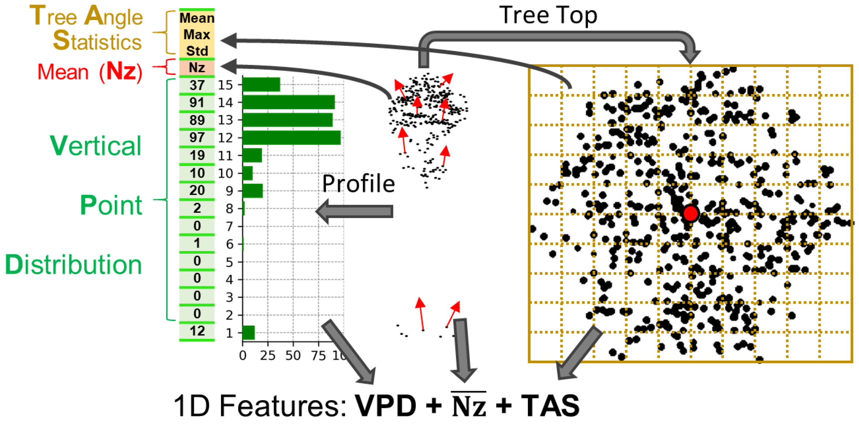
In addition to standard percentile-based features, this study identified the Vertical Point Distribution (VPD) as a particularly effective descriptor. Here, the vertical extent of each crown segment is divided into 15 equally spaced height layers, and the point density in each layer is computed (see Figure 8 left). This number of layers was determined based on experimental evaluation, where various configurations (5, 10, 15, 20, 30, 50 layers) were tested. The setup with 15 layers offered the best balance between resolution and classification accuracy.
Although this method is simple to implement, a review of the literature showed that such layer-based features are rarely used. Most studies rely on selected percentiles (e.g., 90th percentile) or fixed percentile intervals. While related, these approaches differ in information content. In this work, VPD features outperformed percentile-based ones and were therefore defined as a primary feature set.
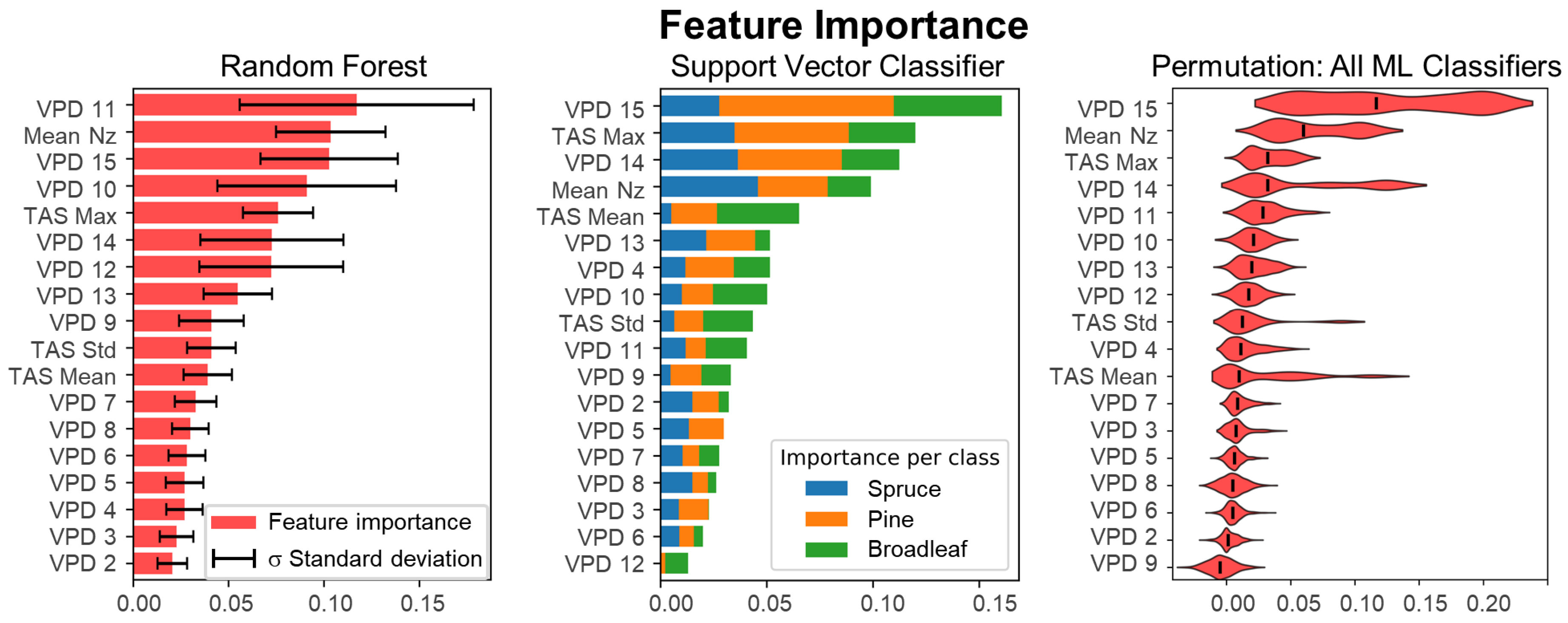
To account for horizontal structure, various statistical descriptors along the x, y, and z axes were tested. However, they did not improve classification performance and were thus excluded from further analysis. A more promising horizontal descriptor was found in the z-component of the surface normals (Nz), as illustrated in Figure 8 middle. When combined with VPD, this feature led to a slight improvement in accuracy. The hypothesis is that Nz captures differences in branch orientation: spruces and pines tend to have more uniformly horizontal branching compared to the more irregular crowns of broadleaf trees.
Taken together, VPD and Nz capture key vertical and horizontal geometric traits of tree crowns. Figure 7 (previous section) also highlights inter-species differences at the tree top level, for instance, conical shapes in spruces, rounded (hyperbolic) tops in broadleaf trees, and intermediate forms in pines.
To statistically represent these shape differences, an additional feature group was developed: Tree Angle Statistics (TAS). As shown in Figure 8 right, a 2D grid was overlaid on each tree segment. For each grid cell containing points, the angle between the tree top (marked as a red point) and the highest point in the cell was computed. From these values, the mean, median, and standard deviation of the angles were derived. These metrics, collectively referred to as TAS, provided a quantitative summary of crown shape and contributed to improved classification performance.
In summary, the 1D feature set includes Vertical Point Distribution (VPD), the z-component of the surface normals (Nz), and Tree Angle Statistics (TAS). Together, these features capture essential aspects of the vertical structure, horizontal orientation, and overall crown shape, providing a compact and effective representation for tree type classification.

3.2.2. ML Algorithms

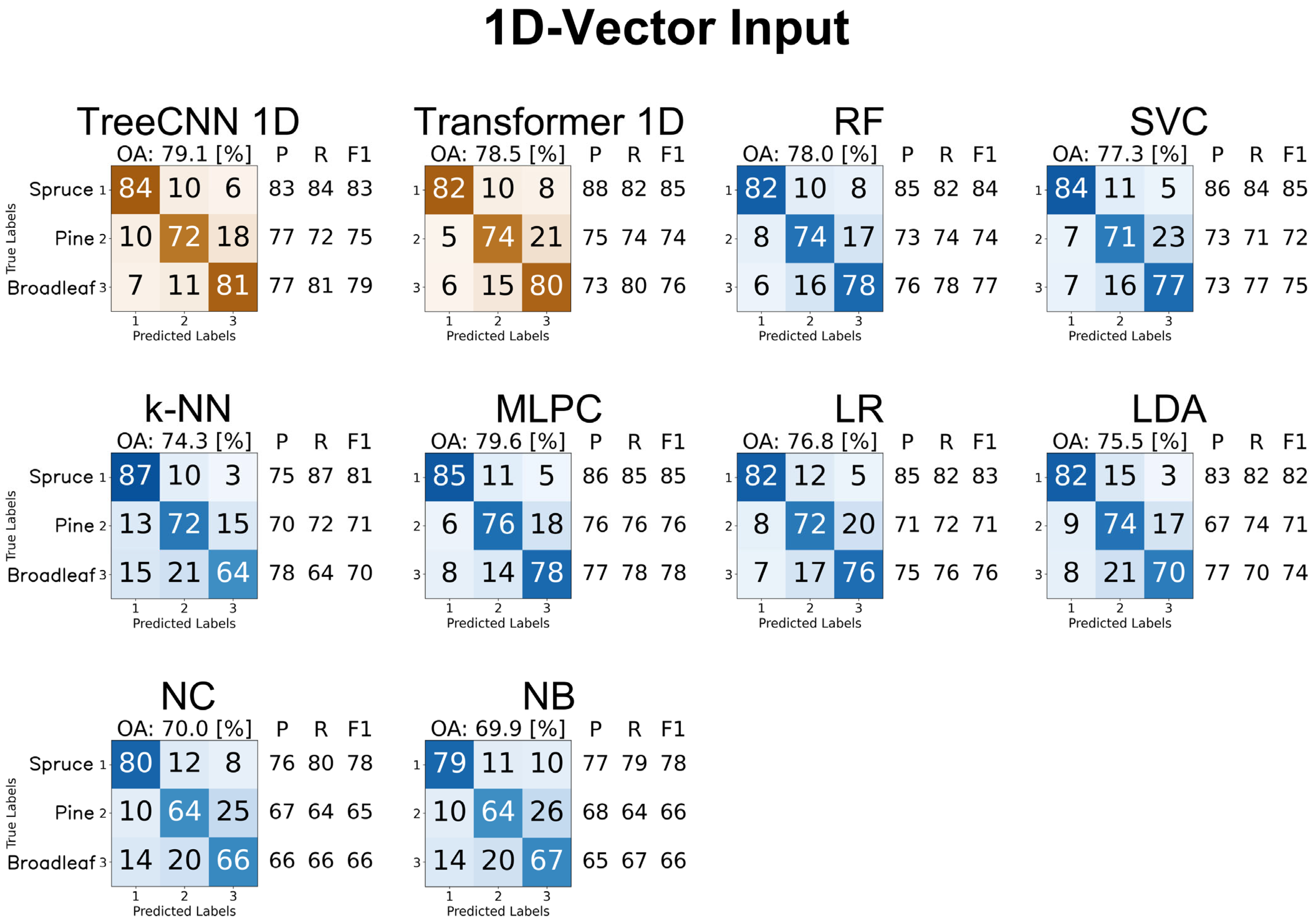
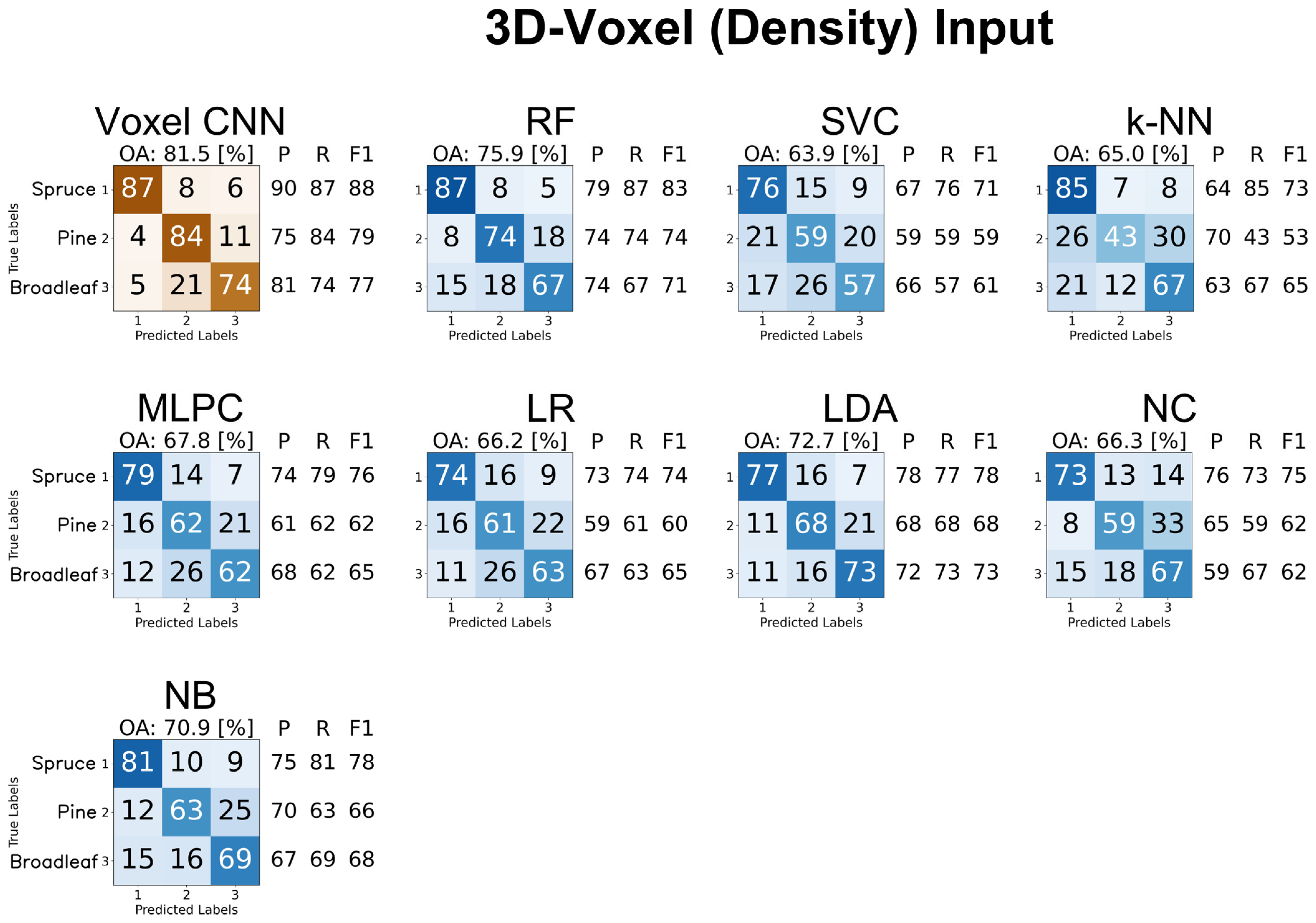
In this study, several commonly used ML algorithms were applied not only to 1D feature representations but also to the 2D and 3D classification approaches (see Table 1).
All ML models were implemented using the scikit-learn library (Version 1.2.2) in Python (Version 3.9.7) (https://scikit-learn.org, accessed on 30 June 2025). While each algorithm provides a set of default parameters optimized for general use, further performance improvements can often be achieved through hyperparameter tuning.
To systematically identify optimal settings, a GridSearch approach was used (https://scikit-learn.org/stable/modules/generated/sklearn.model_selection.GridSearchCV.html, accessed on 30 June 2025). This method evaluates a predefined set of hyperparameter combinations to identify the configuration that maximizes model performance. Only the most influential parameters were adjusted; all others remained at their default values. The selected hyperparameters and their final settings for each algorithm are listed in Table 1.

3.2.3. DL Algorithms

To classify tree types based on the previously extracted 1D features, two Deep Neural Networks (DNNs) were developed: TreeCNN (1D) and Transformer (1D). Both were specifically designed to process low-dimensional feature vectors and optimized for efficient training and inference on standard hardware.
TreeCNN (1D)
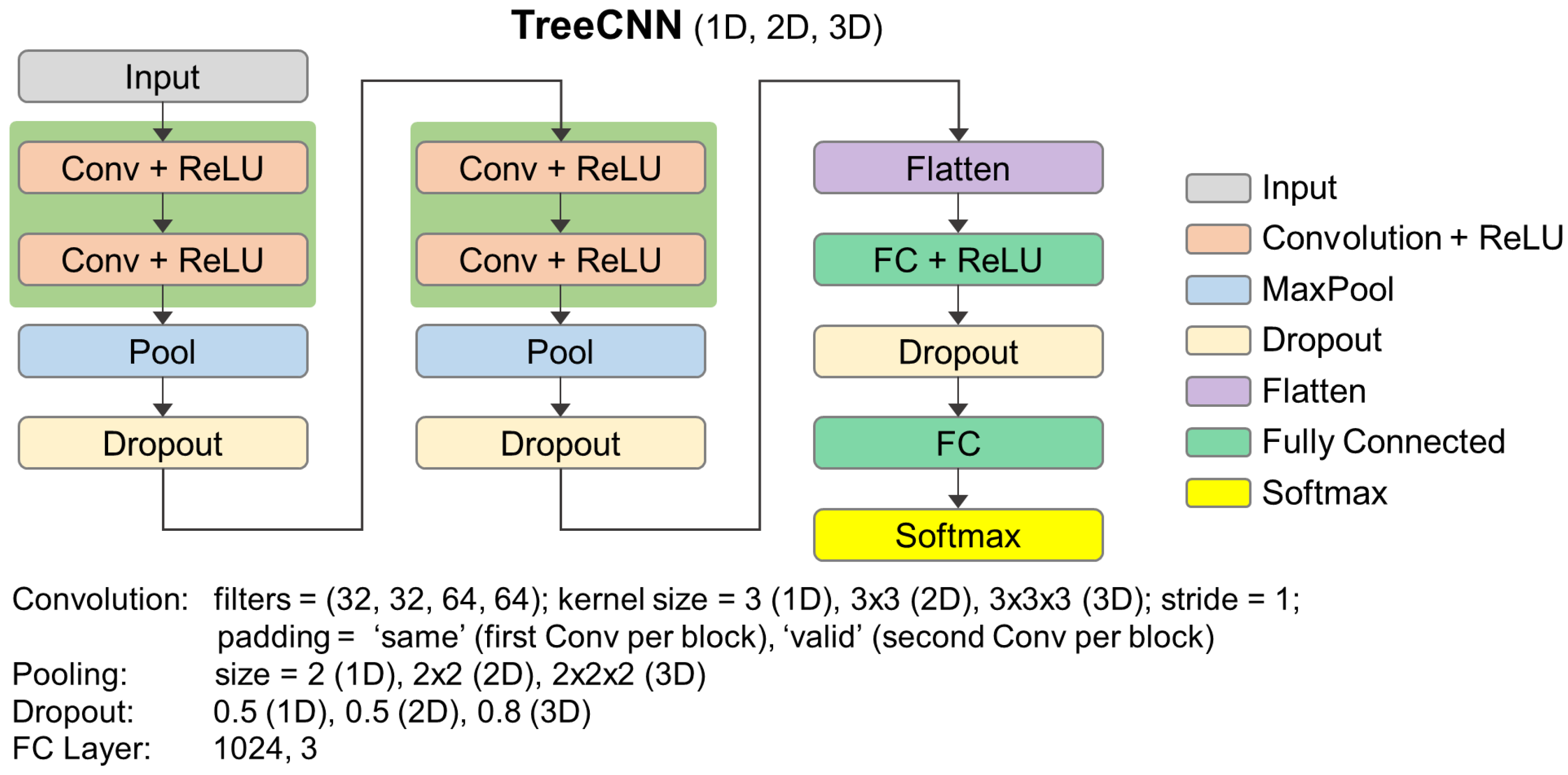
The first model, TreeCNN, is a lightweight 1D CNN (see Figure 9) that shares its core architecture with variants for 2D and 3D data. Only the convolutional and pooling layers are adapted to the respective input dimensionality (e.g., 1D, 2D, 3D), while the overall structure remains unchanged. To reflect this, the network is referred to as TreeCNN_1D, TreeCNN_2D, etc.
The architecture comprises two convolutional blocks, each containing two convolutional layers with Rectified Linear Unit (ReLU) activations. The first block uses 32 filters per layer, the second uses 64. Each block is followed by a max-pooling layer (pool size: 2) and dropout (rate: 0.5). The output is flattened and passed through a Fully Connected (FC) layer with 1024 neurons and ReLU activation, followed by another dropout layer (0.5) and a final FC layer with 3 neurons, corresponding to the tree classes. A softmax layer produces the class probabilities.
TreeCNN_1D was trained using the Root Mean Square Propagation (RMSProp) optimizer (Tensorflow, version 2.6.0) (learning rate: 0.0001, weight decay: 0.00001), with categorical cross-entropy as the loss function and accuracy as the evaluation metric. Models were trained for 2000 epochs with a batch size of 128, using validation-based model checkpointing to retain the best-performing version. Despite its compact architecture (91,000 to nearly 1,000,000 parameters depending on input), TreeCNN_1D achieved competitive accuracy and was designed to run efficiently on Central Processing Unit (CPU)-only systems.
Transformer for 1D Features
The second approach, Transformer (1D), adapts the Transformer architecture—originally developed for natural language processing—to the 1D feature space. Given that the feature vector can be interpreted as a sequence, the self-attention mechanism central to Transformers is well suited to capture complex inter-feature relationships.
Unlike Natural Language Processing (NLP) models, no tokenization or position encoding is needed, as the input features are already numerical and ordered. The Transformer block (Figure 10) consists of Multi-Head Attention (5 heads), followed by dropout (0.1) and Layer Normalization. A Feed-Forward Network (FFN) with a FC layer (dimension = number of input features and ReLU activation) introduces non-linearity. A second dropout (0.1) and another normalization layer complete the block. Residual connections are included to enhance stability and generalization.
The full network begins with a reshape layer to match the required input format, followed by the Transformer block. This is succeeded by a Global Average Pooling layer, dropout (0.15), a FC layer with 20 neurons, another dropout (0.1), and a final FC layer with 3 output neurons and softmax activation.
Training was conducted using the Adam optimizer (Tensorflow, version 2.6.0) (learning rate: 0.0001, beta1 = 0.9, beta2 = 0.999, weight decay = 0.00001), employing the AMSGrad variant for improved convergence stability. The loss function was sparse categorical cross-entropy, with accuracy as the evaluation metric. Models were trained for 2000 epochs with a batch size of 128. Although overfitting was occasionally observed after 800–1000 epochs, extended training sometimes led to stabilization and accuracy gains. Therefore, model checkpoints were again used to retain the best model per run.
Depending on the input size, Transformer (1D) contains between 4300 and 400,000 trainable parameters. Despite its relatively small size, the model achieved strong classification performance, benefiting from the self-attention mechanism’s ability to model complex relationships within the feature space.

3.3. 2D Raster-Based Methods

Although ALS data is inherently three-dimensional, transforming point clouds into 2D raster representations has become a widely used approach. This allows the application of well-established and efficient deep learning methods developed for image data, including both convolutional and transformer-based architectures.
The question arises: What is the most effective method to accurately transform ALS point cloud data of individual tree crown segments into a 2D format? The following section provides a detailed description of the process used to convert the 3D point cloud into a 2D image representation suitable for subsequent deep learning-based classification.

3.3.1. 2D Specific Data Preparation

In many existing approaches, 2D views are generated from point clouds of man-made objects, which can then be fed into neural networks as raster images. This is a relatively simple and effective solution for man-made objects because the surfaces of such 3D objects often follow certain structures, shapes, and regularities.
However, tree crowns generally do not exhibit clear structures and shapes in ALS data, particularly when dealing with medium or low point density ALS data, as is the case in this study. With higher point density, individual branches of a tree are captured in greater detail, which helps to better define the overall structure. When generating a 2D view from a tree, the outer contours of the tree might be recognizable, but the inner structure of the crown and branching patterns are often lost. However, to differentiate between various tree types, it is crucial to preserve the inner tree structure as much as possible in the 2D view. Additionally, all vertical and horizontal properties and relationships within the crown should be maintained to the greatest extent possible.
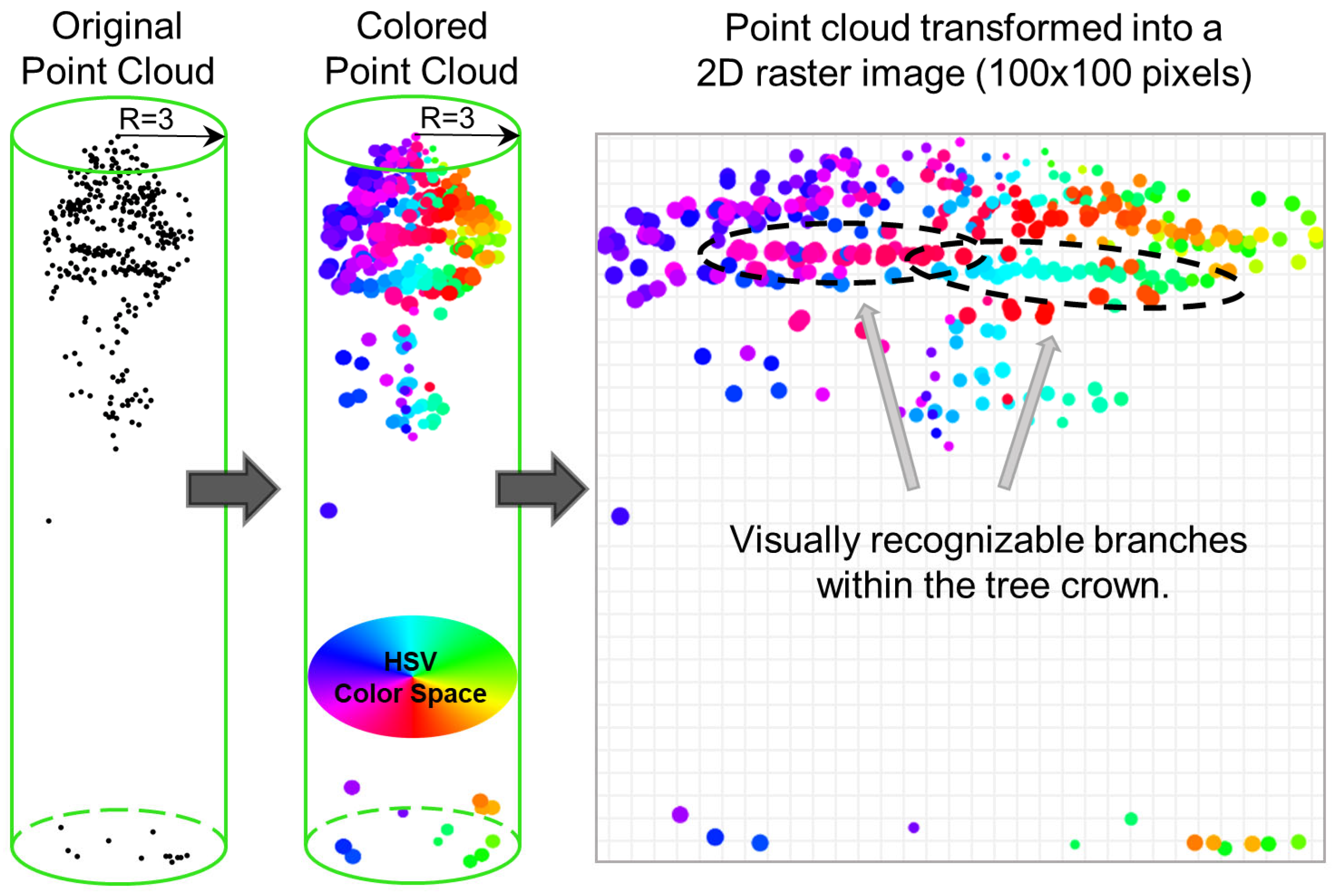
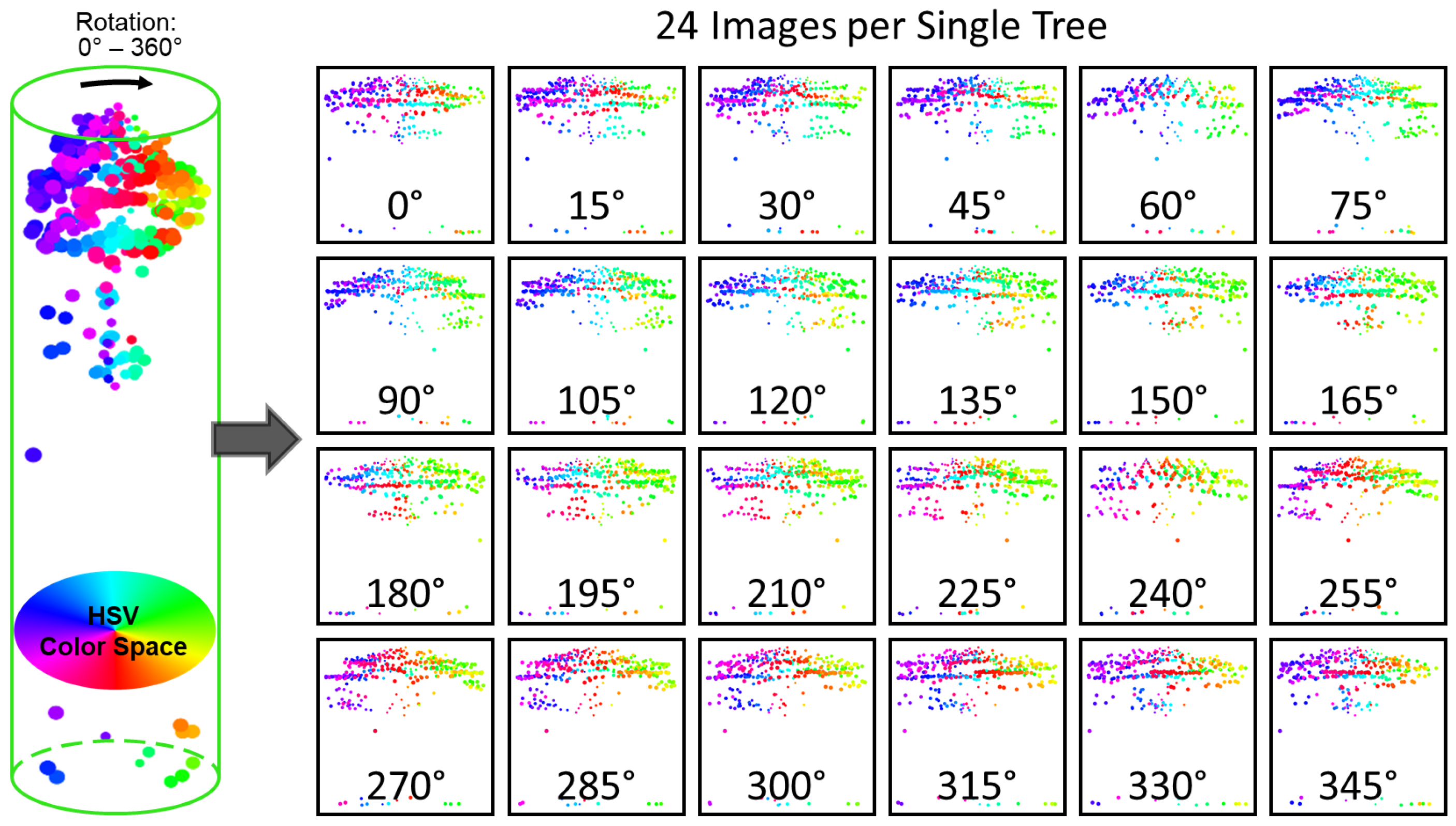
To achieve this, a specialized method for converting tree crown point clouds into 2D views was developed. This specific 2D raster view (Figure 11) is referred to as the “Colored Profile” (CP).
In creating CPs, the 3D points of a tree crown are represented as a type of profile view using symbols (small circles) color-coded in the Hue–Saturation–Value (HSV) color space. While the global orientation of each tree is randomly defined, the color is assigned based on the local orientation of each point relative to the tree top. This color assignment is intended to describe specific branching patterns and forms within the tree crown, from which the model automatically extracts and learns features for classification. Without this color coding, it is difficult to distinguish individual branches or to determine whether a branch is in the foreground or background. All this information is retained in the CP, as shown in Figure 11.
In addition to color variation, the size of the symbols (small circles) also varies. Inner points of a tree crown are depicted slightly smaller compared to outer points. The size of the points is calculated based on their distance (in the xy-plane) in relation to the tree top. This variation in point size prevents excessive overlap of points in the center of the crown, thereby preserving most structures (points are drawn in no particular order, so in the case of overlapping, the color of the last processed point is retained for a given pixel). Experimental results demonstrated that this approach leads to improved classification accuracy due to its ability to capture finer structural details. CPs generated in this manner are saved as square images of 100 × 100 pixel. The decision to use this resolution was based on experimental investigations in which square image resolutions of 5, 10, 20, 50, 100, 150, 225, and 300 pixel were tested. These experiments showed that the chosen resolution offers an optimal balance between detail representation and computational efficiency. Since the trees are much taller relative to the segment width (in this case, a radius of 3 m, as described in Section 3.1.2), the tree crown is effectively “stretched” when transformed into a square image. This effect (see Figure 11) has a positive impact, as horizontally oriented tree structures are represented over a larger area in the image, thus better preserving them.

3.3.2. ML Algorithms

In this section, traditional ML algorithms, as previously described in the 1D vector Section 3.2.2, are utilized for the classification of tree types using 2D CP images. Therefore, the detailed descriptions of the ML algorithms are not repeated here; readers are referred to Section 3.2.2.
To apply these traditional ML algorithms to 2D images, it is necessary to preprocess the images by converting them into 1D feature vectors. This transformation involves flattening the 2D images into a 1D vector by treating each pixel as a separate feature. For instance, a 2D image with dimensions 100 × 100 pixels and 3 color channels (RGB) results in a 1D vector containing 30,000 features.
Typically, in classification tasks involving everyday images, feature identification and extraction are performed manually. Since this has already been accomplished in the 1D vector Section 3.2, this part of the study focuses on evaluating the performance of traditional ML algorithms in classifying tree types using only the previously described CP images and comparing the results to those obtained using DL methods.

3.3.3. DL Algorithms

For the classification based on the previously generated Colored Profiles (CPs), a total of seven DNN architectures were tested, as summarized in Table 2. These networks represent a diverse selection of state-of-the-art models commonly used in computer vision tasks.
The tested DNNs can be categorized into two main groups: convolutional and transformer-based models. The convolutional models include TreeCNN_2D, InceptionV3, Xception, and EfficientNet, all of which are well-established for their efficiency in image classification. In addition, three transformer-based networks—ViT (Vision Transformer), CCT (Compact Convolutional Transformer), and SwinT (Swin Transformer)—were employed. While all three are based on the transformer paradigm, each implements it differently to process 2D visual data.
For all transformer-based models (ViT, CCT, SwinT), standard architecture configurations were used, consistent with the original publications and open-source implementations. The ViT divided the 96 × 96 input images (resized from 100 × 100) into non-overlapping patches of size 6 × 6, resulting in 256 tokens per image. The model used 8 transformer layers, each with 128-dimensional embeddings, 8 attention heads, and an MLP head with two layers of sizes 2048 and 1024. The CCT applied two initial convolutional layers for local feature extraction before passing the representations to 2 transformer blocks with 4 attention heads, embedding dimension 128, and a stochastic depth rate of 0.1. The SwinT used a hierarchical structure with shifted windows, patch size 4 × 4, embedding dimension 128, 8 attention heads, and a lightweight MLP of size 256. These configurations were chosen to reflect a balance between model capacity and computational efficiency, and align with common default setups used in vision-related transformer applications.
Several training parameters were kept consistent across all models, including:
  • Number of training epochs: 50;
  • Batch size: 16;
  • Checkpointing: Best model saved after each epoch.
The optimizer, learning rate, and weight decay values varied slightly depending on the model (see Table 2).
To improve the generalization of the models, various augmentation techniques [62] were tested. The following two augmentation techniques were found to be effective in achieving good generalization and mitigating overfitting:
  • Random zoom adjustments of the input images up to ±10%;
  • Randomly masking 25% of each image by setting the corresponding pixels to white.
The second augmentation technique proved to be particularly useful, as it forced the model during training to achieve optimal classification using the remaining 75% of the image.

3.4. 3D Voxel-Based Methods

In 3D voxel-based methods, unordered point clouds are transformed into an organized voxel structure. This transformation enables more efficient processing and analysis of 3D data, as voxels act as three-dimensional pixels, mapping a space into a grid of discrete units. Each voxel represents a subregion of the studied space and can store various attributes such as density, color, or intensity, depending on the application requirements. By converting to a voxel structure, algorithms for 3D processing tasks can be made more efficient. Compared to methods that operate directly on point clouds, voxel-based techniques ensure uniform data distribution, simplifying calculations. Voxel-based methods particularly facilitate the implementation of ML and DL algorithms by providing a standardized input format.
For tree type classification, point cloud data were converted into two different voxel structures. To process these different voxel structures, specialized neural networks were developed. These networks can recognize and interpret spatial relationships within the voxel structures. Data preparation, design and implementation of these neural networks are discussed in following sections.

3.4.1. 3D Specific Data Preparation

Various approaches have been investigated to effectively transform 3D point clouds into voxel structures. The aim of these efforts was to identify optimal 3D structure to represent unstructured point cloud data. Two voxel structures emerged as particularly promising from these investigations: “Point Density Voxels” and “Binary Voxels”.
Point Density Voxels
The development of this voxel structure involved splitting the point cloud of the tree segment into individual voxels (see Figure 12 left). For each voxel, the point density within the voxel is determined. This parameter is intended to capture the tree structure by describing the distribution of ALS points within the tree canopy. Through careful analysis and experimental investigations, it was found that dividing the tree segment into voxels with dimensions of 4 × 4 × 20 per tree segment provides optimal accuracy for tree type classification. Transforming a tree segment with a radius of 3 m into a voxel structure of 4 × 4 × 20 voxels results in each voxel in the xy-plane representing a division of 1.5 m per voxel. Assuming an average tree height of 30 m, which is evenly divided into 20 layers along the z-axis, this results in a height division of 1.5 m per voxel. Thus, each voxel represents a volume of approximately 1.5 × 1.5 × 1.5 cubic meters of the tree canopy. Although the 4 × 4 × 20 “resolution” is relatively low, it appears to capture the essential details for successful tree type classification. Additionally, it ensures very efficient processing and analysis of the data for both traditional ML and DL.
Binary Voxels
The second method for transforming ALS point clouds into voxel structures, named “Binary Voxels”, aims to capture the distribution of points within the tree canopy as detailed as possible. The core of this method involves dividing the tree canopy into numerous height layers and generating voxels for each of these layers (see Figure 12 right). In contrast to the previous voxel structure, this method defines a much finer voxel structure. These voxels are utilized to store binary information, specifically indicating whether a voxel contains ALS points or not.
Compared to the “Point Density Voxels” structure, the “Binary Voxels” method significantly increases the voxel resolution to 24 × 24 × 50 voxels. With this fine resolution, each voxel represents a volume of approximately 0.25 × 0.25 × 0.60 cubic meters, based on a horizontal division of 0.25 m (for a segment radius of 3 m) and a vertical division of 0.6 m, assuming an average tree height of 30 m. The fine division and small size of the voxels enable a more precise representation of the spatial structure of the tree canopy. This facilitates a comprehensive analysis of the tree canopy and consequently improves tree type classification.
Key Conceptual Difference
The key difference between Point Density Voxels and Binary Voxels goes beyond voxel resolution and lies in how information is represented within each voxel. Point Density Voxels store continuous values that represent the local density of ALS points in each voxel, thereby capturing the internal distribution of points within the tree canopy. In contrast, Binary Voxels encode only the presence or absence of ALS points, using binary values (0 or 1), which reduces the information per voxel but allows for a finer spatial representation of canopy structure. These two voxel types thus represent different trade-offs between data richness and spatial detail, which may influence how effectively various machine learning models can interpret structural patterns in the data.
To account for potential resolution effects, multiple voxel grid configurations were systematically evaluated for both methods, ranging from coarse (e.g., 2 × 2 × 5) to high-resolution setups (e.g., 50 × 50 × 100). In each case, the resolution that yielded the highest classification accuracy was selected. Therefore, the performance of both voxel-based models reflects the representational characteristics of their respective methods, rather than limitations in voxel resolution.

3.4.2. ML Algorithms

In the context of classification using traditional ML methods, the voxel data were directly used as feature lists without extracting specific features. The 3D voxel data were transformed into a one-dimensional structure to serve as input for ML algorithms. This approach, which does not involve further specific feature extraction, is not necessarily optimal for traditional ML methods due to the high number of features. The chosen strategy allows for the evaluation of the effectiveness of traditional ML compared to more advanced DL techniques under comparable conditions. However, due to the suboptimal nature of directly applying high-dimensional voxel data in traditional ML models, it is expected that these models will perform significantly worse.
The same ML algorithms that were employed for 1D and 2D data-based methods were used for 3D voxel-based classification.

3.4.3. DL Algorithms

As part of this study, two DNNs were specifically developed to process the voxel structures resulting from the previous transformation steps, namely “Point Density Voxels” and “Binary Voxels”. These networks, named “VoxelCNN” and “TreeCNN_3D”, were fine tuned to the individualities of their respective data structures. Despite their relatively small size, they are highly efficient and can remarkably operate without the support of Graphics Processing Unit (GPU). This makes the networks particularly resource efficient. Despite their compactness and the ability to operate without specialized hardware, both models achieve notable accuracy in tree type classification due to their careful adaptation to their respective data structures.
VoxelCNN (Figure 12 left) is a compact 3D convolutional neural network developed specifically for processing “Point Density Voxel” representations with input dimensions of 4 × 4 × 20. The architecture is composed of a 3D convolutional layer with 256 filters (3 × 3 × 3, same padding), followed by batch normalization, 3D max pooling, and aggressive regularization through high dropout rates of 0.7. These measures were necessary to counteract overfitting caused by the small input size and limited training data. After feature extraction, the network flattens the spatial data and processes it through a fully connected layer with 1024 neurons before classification via a softmax output layer. VoxelCNN was trained using the Adam optimizer (learning rate: 0.0001, weight decay: 0.00001), with categorical cross-entropy as the loss function and accuracy as the evaluation metric. Although convergence typically occurred within the first 500 of the 1500 training epochs, checkpoints were used to preserve the best-performing model. Despite its minimal size and CPU-efficient design, VoxelCNN achieves strong classification performance due to its targeted design and robust training setup.
TreeCNN_3D (Figure 12 right) is a 3D neural network optimized for the “Binary Voxel” representation and adapted from a previously established 2D architecture. Its extension into the 3D domain involved modifying the convolutional and pooling layers to handle volumetric input while maintaining the simplicity and effectiveness of the original design. To counteract overfitting, a high dropout rate of 0.8 was applied throughout the network (for architectural details and layer parameters, see Figure 9). In addition, a targeted data augmentation strategy was used in which 25% of the input voxels were randomly zeroed out, emulating a 3D “crop out” effect, to further improve model generalization. The network was trained using the AMSGrad variant of the Adam optimizer (learning rate: 0.0001, weight decay: 0.00001) with categorical cross-entropy as the loss function and accuracy as the performance metric. Training was conducted over 150 epochs with a batch size of 16. As with VoxelCNN, a checkpoint mechanism was used to preserve the best-performing model across epochs. Despite the limited dataset and compact design, TreeCNN_3D demonstrates robust classification performance, benefitting from effective regularization and targeted architectural adaptation.

3.5. 3D Point Cloud-Based Methods

For the methods employed in this study, only minimal additional processing is required beyond the basic data preparation outlined in Section 3.1. Therefore, a separate section dedicated to specific data preparation is not needed. Additionally, since traditional ML algorithms cannot directly process point cloud data, only DL algorithms are used in the 3D point cloud-based methods.
A key step in the data preparation involves standardizing the number of points per tree segment. Since most DL algorithms require a uniform number of points per tree segment, the data were processed to standardize the point count across all segments. By calculating the mean and median point counts across all tree segments, an average value of approximately 500 points per segment (by a radius of 3 m) was determined. Based on this insight, datasets with different point densities (384, 512, 1024 points) were prepared. To ensure a consistent number of points across tree segments, randomly selected points were duplicated in segments with fewer points. Equally, if more points were present, a random predefined number of points were selected. This ensured that each dataset had a uniform number of points. Although random sampling could also be performed dynamically during data loading, the preprocessing approach was chosen to ensure consistency and reproducibility across experiments. The conducted investigation showed that point densities of 512 and 1024 yielded the highest accuracies.
During the basic data preparation, the data were already normalized to a range of [−1, +1], eliminating the need for additional preparations. The prepared data in such a way was used for further classification.

DL Algorithms

To classify tree types, two advanced DNNs were employed: PointCNN [51] and the Point Cloud Transformer (PCT) [58]. The adaptation of the PointCNN and PCT architectures for tree type classification involved targeted optimization of model-specific hyperparameters to fully leverage their respective strengths. Both networks were fine-tuned to ensure robust generalization and high classification accuracy, with adjustments made to optimizers, learning rate strategies, and data augmentation techniques.
PointCNN was trained using the Adam optimizer with an ε value of 0.02, which allowed for stable and precise updates of the model weights throughout training. A learning rate scheduling strategy was employed, starting with a base learning rate of 0.01, decaying by a factor of 0.5 every 4000 steps, and incorporating a minimum learning rate threshold. This setup ensured a balanced trade-off between fast initial learning and stable convergence. The core X-Convolution [51] configuration of the original architecture remained unchanged, as empirical tests across 600 training epochs (batch size: 32) confirmed its suitability for the task.
To enhance the model’s robustness and generalization to unseen data, two augmentation techniques were applied: jitter (±0.1) and scaling range (±10% in all three axes). Jitter introduced small random displacements in point positions, while scaling simulated variation in object size. These augmentations, applied to the training data, helped reduce sensitivity to positional noise and structural variation, ultimately improving the model’s ability to handle real-world data variability.
PCT was optimized using the Stochastic Gradient Descent (SGD) optimizer, configured with a learning rate of 0.01, momentum of 0.9, and a weight decay of 0.0005. This combination facilitated efficient convergence while mitigating the risk of overfitting through controlled model complexity. A dropout rate of 0.4 was added to further regularize training.
Additionally, a randomized point selection strategy was applied during training: for each epoch, 75% of the points within each input segment were randomly sampled. This approach, similar to dropout at the input level, prevented over-reliance on specific spatial patterns and improved the model’s generalization capability. PCT was trained over 300 epochs with a batch size of 32, and the best-performing model was retained via checkpointing based on validation performance.

4. Results

The main findings of the classification experiments are presented in three parts. First, the applied validation strategies and evaluation metrics provide the methodological foundation for interpreting model performance. Second, selected visual examples are shown to give an impression of the classification output produced by the Xception model using the 2D data representation. Finally, the quantitative results are analyzed in detail, with a particular focus on systematic comparisons across different input data structures, specifically 1D, 2D, and 3D features, as well as between ML and DL approaches within each structure type. Where appropriate, results are discussed in context to highlight relevant patterns, methodological implications, and practical limitations.

4.1. Validation Methods

To ensure an objective and reliable evaluation of model performance, two widely used validation strategies were applied: a training–validation–test split and K-Fold cross-validation. These approaches assess how well the models generalize to unseen data and help identify potential overfitting.
The training-validation-test strategy involved a fixed partitioning of the data, as described in Section 2.3, and served as the primary method for model evaluation throughout this study.
In addition, K-Fold cross-validation with K values of 5 and 10 was carried out for selected classifiers to verify the reliability of the training-validation-test split used in the main evaluation. This method divides the dataset into K equally sized subsets, training and validating the model K times—each time using a different fold for validation and the remaining folds for training. Averaging the results across folds reduces the variance caused by any single random split and makes efficient use of all available data.
The differences between K-Fold and the fixed split results were small, with only slight increases in overall accuracy (OA) (e.g., 0.32% for K = 5 and 0.54% for K = 10) and moderate increases in standard deviation (1.07% for K = 5 and 1.64% for K = 10). These minor deviations confirm the stability and robustness of the fixed split strategy for the given dataset and task.
Given the marginal performance differences and the substantial computational demands, especially for DL models that require full retraining and hyperparameter optimization for each fold, K-Fold cross-validation was not applied to the complete set of experiments. All further evaluations in this study are therefore based on the training-validation-test split.
To account for variability due to random initialization and training dynamics, all models were trained and evaluated in three independent runs. For consistency and comparability, the run with median overall accuracy was selected to represent each model in the main analysis. This approach reduces the influence of outlier runs while keeping computational demands manageable, particularly for deep learning models.
Model performance was assessed using standard classification metrics: overall accuracy, precision, recall, F1-score, and confusion matrices. These complementary metrics provide a detailed view of classification performance and help identify potential strengths, weaknesses, and misclassification tendencies.

4.2. Illustrative Results

Before presenting the quantitative evaluation, selected visual results are shown to qualitatively illustrate the classification performance and model behavior in a representative test area.
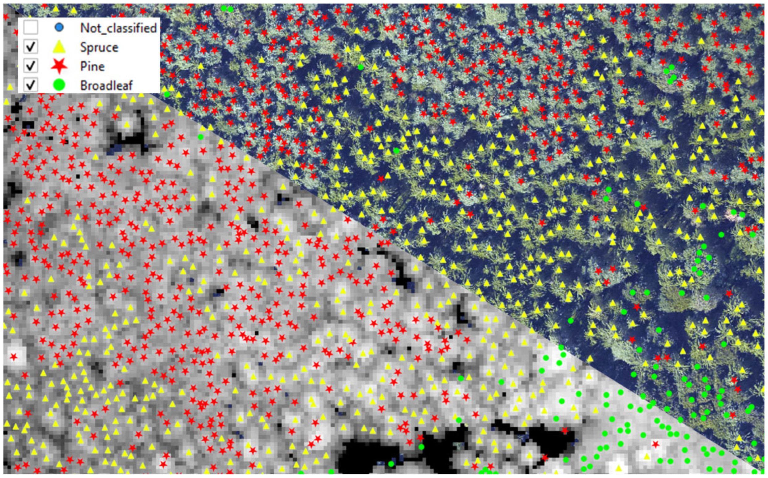
Figure 13 displays a segment of the classification results for spruce, pine, and broadleaf trees, with classified trees shown using distinct symbols and colors. The background is split diagonally: the upper half is overlaid on aerial imagery, while the lower half is shown on a canopy height model derived from ALS data. This dual representation enhances interpretability and supports spatial orientation.
A visual inspection reveals that the majority of trees are successfully detected and accurately classified. This holds true for both isolated trees surrounded by different species as well as for homogeneous clusters. The spatial distribution and classification patterns appear consistent across both types, underlining the robustness of the classification process.
Notably, a concentration of broadleaf trees is visible in the lower right portion of the figure. A closer look reveals a tendency toward over-detection in this class. As discussed previously in Section 3.1.1, this behavior stems from the deliberate tuning of the detection algorithm to minimize false negatives, even at the cost of increased false positives. While this results in multiple detections for some individual broadleaf trees, the correct species label is still assigned in most cases. As such, the over-detection has a negligible impact on classification quality, particularly when aggregating results at larger spatial scales. This is especially true for applications where the total crown area per class is of greater interest than the exact number of individual trees, as long as sub-segments are classified correctly.

4.3. Quantitative Results

To enable a clear and structured comparison across a large number of classification experiments, the results were visualized using a standardized bar chart format. Given the broad variety of tested classifiers (ML and DL), as well as different data structures (1D, 2D, and 3D), an efficient and interpretable form of presentation was essential.
Rather than displaying dozens of individual confusion matrices, each of which provides detailed but isolated insight, the key performance metrics were summarized in comparative bar plots that emphasize the OA of each model (Figure 14). In addition, class-specific accuracies are visualized as smaller sub-bars below each main bar, offering insight into per-class performance without overwhelming the reader.
To enhance readability and facilitate comparison, ML and DL results are clearly differentiated using consistent color schemes and labeling conventions: ML classifiers are represented by fixed acronyms, while DL results are numbered sequentially. This dual labeling approach allows for intuitive navigation both within and across data types and remains effective even in black-and-white print. The graphical grouping of bars reflects the underlying data structure used (e.g., 1D, 2D, or 3D), enabling structured analysis of input-level effects.
This visualization strategy enables direct, side-by-side comparison of dozens of models, allowing trends, strengths, and outliers to be identified at a glance. It is particularly well-suited for classification tasks involving a limited number of classes, as in this study, where three classes were used. The approach remains visually effective for up to approximately five classes; beyond that, readability and interpretability may decrease due to increasing visual complexity.
Figure 14 provides an overview of the classification performance of all tested ML and DL models across the different input data structures and serves as the basis for the following result interpretation. For readers seeking more detailed insights, the full confusion matrices as well as class-wise Precision, Recall, and F1-scores for all models are provided in the Appendix A. These matrices allow for in-depth examination of misclassification patterns and are color-coded to distinguish between ML models (blue-toned) and DL models (red-toned), supporting clear differentiation even in dense result sets.

4.3.1. 1D Feature Vectors

Using handcrafted 1D features, both ML and DL models achieved similar performance. The highest overall accuracy (79.6%) was achieved by MLPC (ML), followed closely by TreeCNN_1D and Transformer_1D (DL). Several other ML algorithms, including RF, SVC, and LR, showed competitive results with only marginal differences.
As shown in Figure 14 (lower part of the graph), spruce trees were classified with the highest accuracy across almost all models. Among the three classes, pine and broadleaf trees were most frequently misclassified as each other, likely due to their similar structural characteristics. This pattern is clearly visible in the confusion matrices provided in Appendix A.

4.3.2. 2D Raster Profiles

When using 2D rasterized tree profiles, DL models clearly outperformed traditional ML methods. The CNN-based model Xception achieved the highest accuracy (85.7%), followed by InceptionV3 and TreeCNN_2D. Transformer-based DL models performed notably worse, suggesting that the 2D profile structure benefits more from localized spatial encoding than from global attention mechanisms.
ML classifiers were limited by the high dimensionality of the input and pixel redundancy. As visible in Figure 14, k-NN performed poorly (approx. 60%) and showed large intra-class variability, again with lower accuracy for broadleaf trees.

4.3.3. 3D Voxel Representations

In voxel-based formats, the DL model VoxelCNN achieved an accuracy of 81.5% using point density voxels. TreeCNN_3D reached just above 79% with binary voxel input. Among the ML models, RF achieved the highest accuracy but remained clearly behind the performance of DL approaches across both voxel types. As shown in Figure 14, DL models—particularly VoxelCNN—benefited substantially from the richer voxel-level information provided by the point density format. To ensure that this advantage was not simply due to differences in voxel resolution, a range of grid configurations was tested for both voxel types, as described in Section 3.4.1, and the reported results are based on the best-performing resolution in each case. While some ML models showed marginal improvement with binary voxel input, their overall performance was consistently and significantly lower than that of DL models. Spruce was once again the most accurately classified class, confirming previous patterns across data structures.

4.3.4. 3D Point Clouds

Direct classification on 3D point clouds yielded the highest overall accuracies (Figure 14). PointCNN achieved 88.1%, followed by PCT with 86.1%. These models directly process unstructured 3D data and thus preserve the full spatial complexity of tree crowns, an advantage not present in voxelized or rasterized formats.
Although all three classes were classified with high accuracy, broadleaf trees showed slightly lower performance compared to spruce and pine, consistent with previous data structures and reflective of their less distinct structural characteristics.

4.3.5. Summary of Results

The results demonstrate that classification performance strongly depends on the chosen data structure and the applied algorithm type. While 1D feature inputs allow both ML and DL models to achieve competitive results, more complex data representations—such as 2D raster, 3D voxel, and 3D point cloud—consistently favor deep learning approaches.
DL models outperformed ML algorithms across all non-1D data structures, with particularly large margins for 2D and 3D inputs. The highest overall accuracy was achieved by point cloud–based models, confirming that minimal preprocessing and full spatial context offer the greatest benefit for tree type classification. The choice of data structure should therefore be aligned with the intended balance between classification performance, model complexity, and computational resources.
Across all data structures and models, spruce trees were classified with the highest reliability, while pine and broadleaf trees exhibited higher confusion rates—particularly with each other—due to structural similarities.

5. Discussion

The classification results presented in the previous section reveal clear dependencies between data structure, model type, and classification performance. In this discussion, we interpret these findings with respect to model behavior, representational choices, and practical applicability. Additionally, we reflect on the limitations of the current study and propose directions for future research.

5.1. Model Behavior and Interpretation

5.1.1. Feature Importance for 1D Data Structure

To gain deeper insights into model behavior on 1D input structures, a feature importance analysis was conducted across all applied ML classifiers. The goal was to identify which handcrafted features contributed most to tree type classification accuracy and whether specific vertical or geometric traits were particularly discriminative.
Feature importance quantifies the contribution of each input variable to the model’s prediction performance. For traditional ML models, this can be assessed using various approaches, including model-intrinsic metrics (e.g., impurity reduction in Random Forests), coefficient magnitudes (in linear models), and permutation-based techniques.
As shown in Figure 15, three complementary methods were applied to assess feature importance: Random Forest importance scores (left), class-specific sensitivity analysis using a Support Vector Classifier (center), and permutation importance across all ML classifiers (right). The permutation results are visualized as violin plots, representing the distribution of importance values for each feature across different models, thereby highlighting consistency and variability in their relevance.
The evaluated 1D feature set consisted of 15 Vertical Point Distribution (VPD) layers, the average z-component of surface Normals (Nz), and three Tree Angle Statistics (TAS), as described in Section 3.2.1. The following patterns summarize consistent findings across all three feature importance analyses:
  • VPD upper layers (especially layers 10–15) had the highest discriminative power across all classifiers. These layers capture structural characteristics near the top of the crown, where ALS point density is highest and species-specific shapes are most distinct.
  • Nz (normal z-component) emerged as a highly informative horizontal descriptor, likely reflecting branching orientation differences, e.g., the uniform horizontal layering in spruce and pine vs. the irregular crowns of broadleaf species.
  • TAS metrics (mean, median, standard deviation of crown surface angles) added complementary geometric information, improving classification, particularly when combined with VPD.
Class-specific patterns were also observed. For example, in the SVC-based classification, the topmost VPD layers were particularly important for distinguishing pine and broadleaf trees, while spruce trees were better characterized by slightly lower layers (VPD 12–13). This aligns with known morphological differences: spruces tend to have more conical, vertically layered crowns, whereas broadleaf and pine crowns are flatter or more irregular.
Interestingly, features from the lower crown layers contributed little to the overall model performance. This is consistent with ALS acquisition geometry: most laser returns originate from the upper canopy layers, and deeper crown regions are often occluded, especially under leaf-on conditions.
While feature importance analysis is relatively straightforward for traditional ML algorithms, its application in DL models is substantially more complex due to the hierarchical and distributed nature of feature representations. Advanced interpretability techniques, such as permutation importance [88], gradient-based saliency methods [89], random forest–based explanation frameworks [90], or local surrogate models like Local Interpretable Model-agnostic Explanations (LIME) [91]—have been developed to address this challenge. However, these methods often involve high computational costs and limited interpretability. Due to these limitations and resource considerations, feature importance analysis in this study was deliberately restricted to 1D feature-based ML classifiers. No equivalent analysis was conducted for 2D or 3D DL models. Nonetheless, the patterns and rankings derived from ML-based importance scores remain highly relevant: since DL classifiers were trained on the same 1D input vectors, it is reasonable to assume that they also rely on similar structural features.

5.1.2. Limitations of ML on 2D-Raster and 3D-Voxel Data Structures

The classification results revealed a consistent pattern: traditional ML algorithms performed significantly worse than DL methods when applied to both 2D raster-based and 3D voxel-based input representations. This performance gap is rooted in how classical ML models interact with high-dimensional and structurally complex data formats.
In the case of 2D Colored Profile (CP) images, the transformation from a structured raster into a flat 1D feature vector results in a dramatic increase in input dimensionality. A single 100 × 100 pixel RGB image produces 30,000 individual features per sample. However, a substantial portion of these pixels correspond to background (i.e., white, empty space), which carries no structural information about the tree crown. The result is a sparse and highly redundant feature space, in which meaningful signals are diluted by non-informative data.
Similarly, 3D voxel structures, especially in fine-resolution formats like the 24 × 24 × 50 binary voxel grids used in this study, lead to thousands of input features per sample when flattened for use in ML algorithms. As with 2D raster data, many of these voxels represent empty space or sparse regions, further exacerbating the problem of irrelevant or redundant features.
In typical ML pipelines, such issues are addressed using dimensionality reduction techniques, such as Principal Component Analysis (PCA) or Linear Discriminant Analysis (LDA) [79,92], to compress the input space and eliminate noise. However, in the present study, dimensionality reduction was deliberately omitted to allow a direct and fair comparison with DL models, which process the full high-dimensional input. This ensured that all approaches were evaluated under identical data conditions.
The consequence of this design choice was that ML models, lacking inductive biases such as spatial locality, translational invariance, or hierarchical abstraction, struggled to extract meaningful patterns from the unfiltered, high-dimensional inputs. Classifiers like k-NN, LR, and even RF performed poorly, particularly for broadleaf trees where crown structure is less distinctive.
In contrast, DL architectures (e.g., CNNs for 2D inputs and VoxelCNN for 3D inputs) are inherently designed to learn localized patterns and hierarchical features, making them vastly more effective in parsing complex spatial representations. These models utilize convolutional operations to focus on structurally relevant regions while ignoring redundant background, leading to improved classification accuracy and better generalization.

5.1.3. Reliability and Probabilistic Confidence

In addition to classification accuracy, the reliability of predicted class probabilities is a critical factor in evaluating model performance. These probabilities reflect how confidently a model assigns a tree to a specific class and are particularly relevant in applications where uncertainty must be quantified or managed.
To explore this aspect, Figure 16 presents violin plots of the predicted probability distributions for the three tree classes (spruce, pine, and broadleaf) across a selection of models. The figure includes seven 2D-based models and two 3D-based models, enabling a direct comparison across input structures. Each violin represents the density of predicted probabilities for a given class and model; narrow, peaked distributions near 1.0 indicate high confidence, while broader or flatter shapes reflect lower certainty or greater variability.
The plotted results reveal several notable patterns:
  • TreeCNN (2D) shows high reliability for spruce, with probabilities clustered near 1.0. However, predictions for pine and broadleaf are more dispersed, indicating lower confidence and greater uncertainty in these classes.
  • The InceptionV3, Xception, and PointCNN (3D) models exhibit very narrow distributions near 1.0 for all three classes. These models provide consistently high prediction confidence.
  • CCT (2D) and SVC (2D) demonstrate moderate confidence, with predicted probabilities typically ranging from 0.6 to 0.9. Notably, SVC exhibits slightly broader distributions for pine and broadleaf, suggesting more variability and lower certainty for these more ambiguous classes.
  • ViT (2D) and PCT (3D) fall into an intermediate range. Both show peaked but wider distributions, particularly for pine, reflecting moderate confidence in predictions. Between the two, PCT tends to produce slightly higher median probabilities, particularly for spruce.
  • RF (2D) displays the least reliable outputs, with all three classes showing broad, flat distributions and the lowest median probabilities. This suggests a general tendency toward low certainty and less discriminative output compared to DL models.
Overall, the figure underscores a consistent trend: DL models, especially CNN-based architectures and 3D point cloud methods, produce more confident and better-calibrated predictions than traditional ML classifiers. Among them, InceptionV3, Xception, and PointCNN stand out for their high confidence and low variability across all classes.
These results also highlight the inherent uncertainty in classifying pine and broadleaf trees, which tend to exhibit overlapping structural characteristics. Even well-performing models show slightly broader distributions for these classes compared to spruce, which remains the most reliably classified across all models.

5.2. Ensemble Modeling

Ensemble methods are widely used in machine learning to improve classification accuracy by combining the outputs of multiple models. In this study, two ensemble strategies were evaluated:
  • Intra-structure ensembles, combining models of the same data type (e.g., multiple 2D-based models);
  • Cross-structure ensembles, combining models across different data representations (e.g., 1D, 2D, and 3D).
For both strategies, soft voting (averaging class probabilities) and hard voting (majority class selection) were tested. However, the results showed that these approaches yield only marginal improvements, typically no more than 1–2% in overall accuracy. Importantly, accuracy gains were observed only when top-performing models were carefully selected. Including lower-performing models in the ensemble often led to no improvement or even a decrease in accuracy, highlighting the risk of combining heterogeneous or suboptimal classifiers without additional selection criteria.
To further investigate ensemble potential, an alternative approach was tested: instead of relying on voting, a meta-model was trained to predict the final class based on the class probabilities produced by individual models. This method, essentially a stacked ensemble, aimed to learn which models are most reliable under specific conditions. While conceptually promising, this approach also resulted in only slight and inconsistent improvements, performing similarly to soft voting and, in most cases, not surpassing the accuracy of the best single model in the ensemble.
These findings indicate that the limited impact of ensemble methods may stem from several interacting factors. First, although different data structures were used, the individual models appear to converge on similar decision boundaries, suggesting limited model diversity. Second, the limited improvement suggests that many of the misclassifications were shared across models reducing the benefit of combining their predictions. Third, ALS-based representations may inherently lack the class-specific separability needed to fully exploit ensemble learning. Taken together, these factors suggest that performance ceilings were not primarily due to the ensemble strategy itself, but rather to the representational capacity of the ALS data and the nature of the classification task.

5.3. Accuracy Improvement Using Multi-View Profiles (MVPs) of a Single Tree

The results presented so far for 2D data structures were based on using a single profile view per tree crown during inference. This raises the question whether classification accuracy can be further improved by systematically incorporating multiple views of the same tree. The idea behind this approach—referred to as Multi-View Profiles (MVPs)—is to enhance structural representation by rotating the tree crown and generating additional 2D perspectives (see Figure 17).
In this study, 24 profile views per tree were generated at 15° rotation intervals. Although all views were used for data augmentation during training, inference in the main experiments relied only on a single profile per tree. To explore the benefit of aggregating multiple views during prediction, an additional experiment was conducted in which the predicted class probabilities from multiple views were combined via soft voting—averaging the probabilities across all selected views to determine the final class label.
The impact of this approach is summarized in Figure 18, which shows accuracy improvements for several representative models. The results indicate consistent performance gains across all tested models, with improvements ranging from 1.8% to over 6%, depending on the model architecture and number of views used.
The observed accuracy improvements follow a consistent pattern across models:
  • The largest gains occurred when combining the first few additional views. On average, adding just one more profile led to a 1–3% accuracy increase.
  • After approximately eight views, the improvement curve began to flatten, suggesting that the most relevant structural information is captured within the first 8 orientations.
  • Transformer-based DL models (e.g., ViT, CCT) exhibited the highest relative gains (4–6.5%), supporting the hypothesis that they benefit more from larger and more diverse input distributions, possibly compensating for limited training data.
  • CNN-based models (e.g., Xception, TreeCNN) and traditional ML classifiers (e.g., RF, SVC) also benefited, though with smaller relative gains (1.5–3.5%).
These findings demonstrate that MVPs effectively function as a form of ensemble learning, where multiple weaker predictions are aggregated into a more robust final decision. Notably, the Xception model achieved 85.7% accuracy with a single profile, and 88.1% when using eight profiles, matching the performance of point cloud–based models such as PointCNN.
This convergence suggests that 2D CNN models can achieve comparable accuracy to PCL methods, but only if multiple MVPs are used during inference. However, this advantage comes with trade-offs: although 2D models are architecturally simpler and require less memory, the need to process multiple inputs per tree significantly increases inference time. In practice, using eight profiles per tree can offset the runtime advantage and may even render 2D approaches slower than well-optimized PCL-based methods. Therefore, the choice between 2D + MVP and native 3D approaches should be based not only on classification accuracy, but also on available hardware, computational efficiency, and specific application requirements.

5.4. Implications for Application and Method Selection

The results of this study provide clear guidance for selecting suitable methods depending on the specific application context. When computational resources are limited or model transparency is prioritized, traditional ML models using 1D handcrafted features offer acceptable performance with low complexity. In contrast, DL models trained on 3D point clouds achieve the highest accuracy and are better suited for precision-critical applications such as ecological monitoring or inventory systems.
Intermediate representations (e.g., 2D raster images or 3D voxels) may offer a trade-off between accuracy, interpretability, and computational demand. For use cases where per-tree predictions are required at scale, 2D models combined with MVP-based inference present a viable alternative, albeit with longer inference times.
Spruce trees were consistently easier to classify due to their distinct structural properties, while pine and broadleaf classes showed more overlap, highlighting the importance of species-specific modeling strategies.

5.5. Limitations and Future Directions

One major limitation of this study is its focus on a geographically and compositionally restricted dataset, covering only three tree types within a single forest region. Although the dataset was standardized and balanced to ensure fair model comparisons, the results cannot be directly generalized to more diverse forest types, stand structures, or ecological conditions. This consequently limits the transferability of the trained models and affects how the reported classification accuracies should be interpreted. Additionally, the reliance on manually annotated training data limits scalability and may introduce subjective bias in class definitions and labeling consistency.
To improve generalizability and reduce annotation overhead, future work should explore semi-automatic labeling strategies, active learning, or weak supervision frameworks. These approaches can help expand dataset size and diversity while minimizing manual effort.
Basic data augmentation techniques such as geometric transformations (e.g., cropping, scaling, jittering) and multi-view sampling (see Section 5.3) were already applied during training to introduce structural variation and improve model robustness. However, there remains substantial untapped potential for augmentation to enhance model transferability across different regions and forest types. Looking ahead, more advanced augmentation strategies could be explored to further enhance generalizability and transferability. For instance, guided augmentation based on species-specific crown shapes (e.g., conical for spruce vs. rounded for broadleaf), branching patterns, or vertical crown profiles could help simulate variability across different regions, forest compositions, and stand densities. Additionally, synthetic crown generation using generative models could replicate structurally diverse trees from different ecological conditions. While such techniques cannot fully replace external validation, they represent a practical and scalable means of improving model robustness and mitigating the effects of regional variability in deep learning-based forest classification.
Another promising direction is the use of multi-temporal ALS data, which has the potential to capture phenological variation and subtle structural changes over time. Such temporal dynamics could improve classification robustness, particularly for classes with overlapping static structures, such as pine and broadleaf trees.
Beyond the use of purely geometric information, the integration of spectral attributes from LiDAR systems themselves presents a promising direction. Even conventional ALS systems provide intensity values that reflect surface reflectance properties at the laser wavelength, offering valuable information beyond 3D structure. More advanced multispectral LiDAR systems extend this by capturing wavelength-dependent reflectance across multiple channels, potentially enabling more nuanced species differentiation. In this context, combining different input modalities directly at the data level, for example, by concatenating geometric and spectral features into a joint representation, offers a simple yet effective fusion strategy. This form of early fusion requires minimal architectural adaptation and can be easily applied across various model types.
Preliminary results indicate that combining ALS data with either multi-temporal information or intensity data can lead to consistent improvements in classification accuracy across different data structures and model types. These findings highlight the potential of integrating complementary data sources and suggest that further research should focus on systematic multimodal and temporal fusion, particularly through straightforward strategies such as feature-level combination, to enhance model robustness in operational forest classification tasks.

6. Conclusions

This study systematically investigated the classification of individual tree types using ALS data in a structurally complex and ecologically diverse Central European forest. By comparing multiple data representations—from handcrafted 1D feature vectors to 2D rasterized profiles and 3D voxel and point cloud structures—and evaluating both traditional Machine Learning (ML) and Deep Learning (DL) models, we were able to provide a comprehensive assessment of the effectiveness of different approaches.
The results clearly demonstrate that DL models consistently outperform classical ML methods when applied to 2D and 3D data structures. Highest classification accuracy was achieved using 3D point cloud data in combination with DL models (e.g., PointCNN), highlighting the advantages of preserving the full geometric complexity of individual tree crowns. While handcrafted 1D features still yielded competitive results, particularly when using well-designed vertical descriptors, their performance reached a limit when compared to higher-dimensional representations, especially in distinguishing structurally similar classes such as pine and broadleaf trees.
2D raster-based methods, particularly when enhanced with Multiple View Profiles (MVPs), also proved effective, achieving classification accuracies comparable to 3D models. However, this came at the cost of increased inference time and complexity. Voxel-based models, while less accurate than 3D point cloud-based methods, offered a valuable compromise between data regularization and spatial resolution.
Across all methods, classification accuracy was highest for spruce trees, likely due to their distinct, vertically structured crowns. Confusion between pine and broadleaf trees remained a challenge across representations and models, underlining the limitations of structural ALS data alone in separating morphologically similar species groups.
From a practical standpoint, the choice of data representation and model should be guided by the specific constraints and goals of the application. In resource-limited scenarios, 1D ML approaches remain viable. For high-precision applications, DL models based on 3D point clouds or MVP-enhanced 2D profiles are recommended.
Future work should extend this analysis to more diverse forest types, integrate additional data sources (e.g., multi-temporal ALS or intensity information), and explore multimodal fusion strategies to improve robustness and scalability. Particularly promising are methods that combine structural and spectral information at the feature level, which can be applied flexibly across different model architectures.
In summary, this study provides a detailed comparison of methods for tree type classification using ALS data and highlights the trade-offs between data complexity, computational cost, and classification performance. The findings offer both methodological insights and practical recommendations for operational forest mapping and ecological monitoring.

Author Contributions

Conceptualization, S.M. and M.S.; methodology, S.M.; software, S.M.; validation, S.M.; formal analysis, S.M.; investigation, S.M.; resources, S.M. and M.S.; data curation, S.M. and M.S.; writing—original draft preparation, S.M.; writing—review and editing, M.S. and R.P.; visualization, S.M.; supervision, M.S. and R.P.; project administration, M.S.; funding acquisition, M.S. All authors have read and agreed to the published version of the manuscript.

Funding

This research received no external funding.

Data Availability Statement

The datasets presented in this article are not readily available because they belong to companies.

Acknowledgments

The test data used in this study stem from JOANNEUM RESEARCH and AeroMap. During the preparation of this manuscript, the authors used ChatGPT (GPT-4o) for the purposes of translations. The authors have reviewed and edited the output and take full responsibility for the content of this publication.

Conflicts of Interest

Authors Sead Mustafić and Roland Perko was employed by the company JOANNEUM RESEARCH Forschungsgesellschaft mbH. The remaining authors declare that the research was conducted in the absence of any commercial or financial relationships that could be construed as a potential conflict of interest.

Abbreviations

The following abbreviations are used in this manuscript:
ALSAirborne Laser Scanning
CCTCompact Convolutional Transformer
CHMCanopy Height Model
CIRColor-Infrared
CNNConvolutional Neural Network
CPColored Profile
CPUCentral Processing Unit
DBHDiameter at Breast Height
DLDeep Learning
DNNDeep Neural Network
FCFully Connected
FFNFeed-Forward Network
GPSGlobal Positioning System
GPUGraphics Processing Unit
Hmeanmean Height
HpHeight percentiles
HSVHue–Saturation–Value
IDIdentifier
ITDIndividual Tree Detection
k-NNk-Nearest Neighbors
LDALinear Discriminant Analysis
LiDARLight Detection And Ranging
LIMELocal Interpretable Model-agnostic Explanations
LRLogistic Regression
MLMachine Learning
MLPCMultilayer Perceptron Classifier
MVPMulti-View Profiles
NBNaive Bayes Classifier
NCNearest Centroid
nDSMnormalized Digital Surface Model
NIRNear-Infrared
NLPNatural Language Processing
NzNormal vector component in the z-direction
OAOverall Accuracy
PCAPrincipal Component Analysis
PCTPoint Cloud Transformer
ReLURectified Linear Unit
RFRandom Forest
RGBRed–Green–Blue
RMSPropRoot Mean Square Propagation
SGDStochastic Gradient Descent
SVCSupport Vector Classifier
SVMSupport Vector Machines
SwinTSwin Transformer
TASTree Angle Statistic
ViTVision Transformer
VPDVertical Point Distribution

Appendix A

Figure A1. Confusion matrices for tree type classification based on 1D feature vectors derived from ALS data. The figure compares ten models: two deep learning approaches (TreeCNN, Transformer—shown in reddish color) and eight machine learning classifiers (Random Forest, SVC, k-NN, MLPC, Logistic Regression, Linear Discriminant Analysis, Nearest Centroid, Naive Bayes—shown in blue tones). Overall accuracy (OA), precision (P), recall (R), and F1-score are reported for each class (1 = Spruce, 2 = Pine, 3 = Broadleaf).
Remotesensing 17 02847 g0a1
Figure A2. Confusion matrices for tree type classification based on 2D rasterized crown profiles derived from ALS data. The figure compares fifteen models: seven deep learning approaches (TreeCNN, InceptionV3, Xception, EfficientNet, ViT, CCT, SwinT—shown in reddish color) and eight machine learning classifiers (Random Forest, SVC, k-NN, MLPC, Logistic Regression, Linear Discriminant Analysis, Nearest Centroid, Naive Bayes—shown in blue tones). Overall accuracy (OA), precision (P), recall (R), and F1-score are reported for each class (1 = Spruce, 2 = Pine, 3 = Broadleaf).
Remotesensing 17 02847 g0a2
Figure A3. Confusion matrices for tree type classification based on 3D voxelized density representations derived from ALS data. The figure compares nine models: one deep learning approach (Voxel CNN—shown in reddish color) and eight machine learning classifiers (Random Forest, SVC, k-NN, MLPC, Logistic Regression, Linear Discriminant Analysis, Nearest Centroid, Naive Bayes—shown in blue tones). Overall accuracy (OA), precision (P), recall (R), and F1-score are reported for each class (1 = Spruce, 2 = Pine, 3 = Broadleaf).
Remotesensing 17 02847 g0a3
Figure A4. Confusion matrices for tree type classification based on 3D binary voxel representations derived from ALS data. The figure compares nine models: one deep learning approach (TreeCNN—shown in reddish color) and eight machine learning classifiers (Random Forest, SVC, k-NN, MLPC, Logistic Regression, Linear Discriminant Analysis, Nearest Centroid, Naive Bayes—shown in blue tones). Overall accuracy (OA), precision (P), recall (R), and F1-score are reported for each class (1 = Spruce, 2 = Pine, 3 = Broadleaf).
Remotesensing 17 02847 g0a4
Figure A5. Confusion matrices for tree type classification based on 3D point cloud data. The figure shows results for two deep learning models (PointCNN and PCTformer—both shown in reddish color), applied directly to segmented individual tree point clouds. Overall accuracy (OA), precision (P), recall (R), and F1-score are reported for each class (1 = Spruce, 2 = Pine, 3 = Broadleaf). Traditional machine learning classifiers are not shown here, as they cannot be applied directly to unstructured point cloud data without prior feature extraction or voxelization steps, which were already evaluated in previous representations.
Remotesensing 17 02847 g0a5

References

  1. Leuschner, C.; Homeier, J. Global Forest Biodiversity: Current State, Trends, and Threats. In Progress in Botany; Lüttge, U., Cánovas, F.M., Risueño, M.-C., Leuschner, C., Pretzsch, H., Eds.; Springer International Publishing: Cham, Switzerland, 2023; Volume 83, pp. 125–159. ISBN 978-3-031-12782-3. [Google Scholar]
  2. Merritt, M.; Maldaner, M.E.; de Almeida, A.M.R. What Are Biodiversity Hotspots? Front. Young Minds 2019, 7, 29. [Google Scholar] [CrossRef]
  3. Hyde, P.; Dubayah, R.; Peterson, B.; Blair, J.B.; Hofton, M.; Hunsaker, C.; Knox, R.; Walker, W. Mapping Forest Structure for Wildlife Habitat Analysis Using Waveform Lidar: Validation of Montane Ecosystems. Remote Sens. Environ. 2005, 96, 427–437. [Google Scholar] [CrossRef]
  4. Li, J.; Hu, B.; Noland, T.L. Classification of Tree Species Based on Structural Features Derived from High Density LiDAR Data. Agric. For. Meteorol. 2013, 171–172, 104–114. [Google Scholar] [CrossRef]
  5. Luo, S.; Wang, C.; Xi, X.; Nie, S.; Fan, X.; Chen, H.; Ma, D.; Liu, J.; Zou, J.; Lin, Y.; et al. Estimating Forest Aboveground Biomass Using Small-Footprint Full-Waveform Airborne LiDAR Data. Int. J. Appl. Earth Obs. Geoinf. 2019, 83, 101922. [Google Scholar] [CrossRef]
  6. Yao, W.; Krzystek, P.; Heurich, M. Tree Species Classification and Estimation of Stem Volume and DBH Based on Single Tree Extraction by Exploiting Airborne Full-Waveform LiDAR Data. Remote Sens. Environ. 2012, 123, 368–380. [Google Scholar] [CrossRef]
  7. Hyyppa, J.; Kelle, O.; Lehikoinen, M.; Inkinen, M. A Segmentation-Based Method to Retrieve Stem Volume Estimates from 3-D Tree Height Models Produced by Laser Scanners. IEEE Trans. Geosci. Remote Sens. 2001, 39, 969–975. [Google Scholar] [CrossRef]
  8. Leutner, B.F.; Reineking, B.; Müller, J.; Bachmann, M.; Beierkuhnlein, C.; Dech, S.; Wegmann, M. Modelling Forest α-Diversity and Floristic Composition—On the Added Value of LiDAR plus Hyperspectral Remote Sensing. Remote Sens. 2012, 4, 2818–2845. [Google Scholar] [CrossRef]
  9. Amiri, N.; Yao, W.; Heurich, M.; Krzystek, P.; Skidmore, A.K. Estimation of Regeneration Coverage in a Temperate Forest by 3D Segmentation Using Airborne Laser Scanning Data. Int. J. Appl. Earth Obs. Geoinf. 2016, 52, 252–262. [Google Scholar] [CrossRef]
  10. Hasenauer, H. Ein Einzelbaumwachstumssimulator für Ungleichaltrige Fichten-, Kiefern- und Buchen-Fichtenmischbestände; Forstliche Schriftenreihe Universität für Bodenkultur: Vienna, Austria; Österr. Ges. für Waldökosystemforschung und Experimentelle Baumforschung: Vienna, Austria, 1994; ISBN 978-3-900865-07-8. [Google Scholar]
  11. Kraus, K. Photogrammetrie: Geometrische Informationen Aus Photographien Und Laserscanneraufnahmen; De Gruyter Lehrbuch, De Gruyter: Berlin, Germany, 2012; ISBN 978-3-11-090803-9. [Google Scholar]
  12. Næsset, E. Effects of Different Sensors, Flying Altitudes, and Pulse Repetition Frequencies on Forest Canopy Metrics and Biophysical Stand Properties Derived from Small-Footprint Airborne Laser Data. Remote Sens. Environ. 2009, 113, 148–159. [Google Scholar] [CrossRef]
  13. Budei, B.C.; St-Onge, B.; Hopkinson, C.; Audet, F.-A. Identifying the Genus or Species of Individual Trees Using a Three-Wavelength Airborne Lidar System. Remote Sens. Environ. 2018, 204, 632–647. [Google Scholar] [CrossRef]
  14. Lindberg, E.; Briese, C.; Doneus, M.; Hollaus, M.; Schroiff, A.; Pfeifer, N. Multi-Wavelength Airborne Laser Scanning for Characterization of Tree Species. In Proceedings of the SilviLaser 2015: 14th Conference on Lidar Applications for Assessing and Managing Forest Ecosystems, La Grande Motte, France, 28–30 September 2015. [Google Scholar]
  15. Yu, X.; Hyyppä, J.; Litkey, P.; Kaartinen, H.; Vastaranta, M.; Holopainen, M. Single-Sensor Solution to Tree Species Classification Using Multispectral Airborne Laser Scanning. Remote Sens. 2017, 9, 108. [Google Scholar] [CrossRef]
  16. Briechle, S.; Krzystek, P.; Vosselman, G. Classification of Tree Species and Standing Dead Trees by Fusing UAV-Based Lidar Data and Multispectral Imagery in the 3D Deep Neural Network Pointnet++. ISPRS Ann. Photogramm. Remote Sens. Spat. Inf. Sci. 2020, V-2–2020, 203–210. [Google Scholar] [CrossRef]
  17. Zhang, C.; Qiu, F. Mapping Individual Tree Species in an Urban Forest Using Airborne Lidar Data and Hyperspectral Imagery. Photogramm. Eng. Remote Sens. 2012, 78, 1079–1087. [Google Scholar] [CrossRef]
  18. Holmgren, J.; Persson, Å. Identifying Species of Individual Trees Using Airborne Laser Scanner. Remote Sens. Environ. 2004, 90, 415–423. [Google Scholar] [CrossRef]
  19. Vaughn, N.R.; Moskal, L.M.; Turnblom, E.C. Tree Species Detection Accuracies Using Discrete Point Lidar and Airborne Waveform Lidar. Remote Sens. 2012, 4, 377–403. [Google Scholar] [CrossRef]
  20. Yu, X.; Litkey, P.; Hyyppä, J.; Holopainen, M.; Vastaranta, M. Assessment of Low Density Full-Waveform Airborne Laser Scanning for Individual Tree Detection and Tree Species Classification. Forests 2014, 5, 1011–1031. [Google Scholar] [CrossRef]
  21. Zhang, C.; Zhou, J.; Wang, H.; Tan, T.; Cui, M.; Huang, Z.; Wang, P.; Zhang, L. Multi-Species Individual Tree Segmentation and Identification Based on Improved Mask R-CNN and UAV Imagery in Mixed Forests. Remote Sens. 2022, 14, 874. [Google Scholar] [CrossRef]
  22. Vermeer, M.; Hay, J.A.; Völgyes, D.; Koma, Z.; Breidenbach, J.; Fantin, D.S.M. Lidar-Based Norwegian Tree Species Detection Using Deep Learning. arXiv 2023, arXiv:2311.06066. [Google Scholar] [CrossRef]
  23. Zhao, K.; Popescu, S. Hierarchical Watershed Segmentation of Canopy Height Model for Multi-Scale Forest Inventory. In Proceedings of the ISPRS Workshop on Laser Scanning, Espoo, Finland, 12–14 September 2007; pp. 12–14. [Google Scholar]
  24. Wang, Y.; Weinacker, H.; Koch, B.; Sterenczak, K. Lidar Point Cloud Based Fully Automatic 3D Single Tree Modelling in Forest and Evaluations of the Procedure. Int. Arch. Photogramm. Remote Sens. Spat. Inf. Sci. 2008, 37, 45–51. [Google Scholar]
  25. Harikumar, A.; Bovolo, F.; Bruzzone, L. A Local Projection-Based Approach to Individual Tree Detection and 3-D Crown Delineation in Multistoried Coniferous Forests Using High-Density Airborne LiDAR Data. IEEE Trans. Geosci. Remote Sens. 2019, 57, 1168–1182. [Google Scholar] [CrossRef]
  26. Williams, J.; Schönlieb, C.-B.; Swinfield, T.; Lee, J.; Cai, X.; Qie, L.; Coomes, D.A. 3D Segmentation of Trees Through a Flexible Multiclass Graph Cut Algorithm. IEEE Trans. Geosci. Remote Sens. 2020, 58, 754–776. [Google Scholar] [CrossRef]
  27. Wack, R.; Schardt, M.; Lohr, U.; Barrucho, L.; Oliveira, T. Forest Inventory for Eucalyptus Plantations Based on Airborne Laserscanner Data. In Proceedings of the ISPRS Workshop 3-D Reconstruction from Airborne Laserscanner and InSAR Data, Dresden, Germany, 8–10 October 2003; pp. 40–46. [Google Scholar]
  28. Wack, R.; Stelzl, H. Assessment of Forest Stand Parameters from Laserscanner Data in Mixed Forests. Proc. For. 2005, 56–60. [Google Scholar]
  29. Persson, Å.; Holmgren, J.; Söderman, U. Detecting and Measuring Individual Trees Using an Airborne Laser Scanner. Photogramm. Eng. Remote Sens. 2002, 68, 925–932. [Google Scholar]
  30. Hamraz, H.; Jacobs, N.B.; Contreras, M.A.; Clark, C.H. Deep Learning for Conifer/Deciduous Classification of Airborne LiDAR 3D Point Clouds Representing Individual Trees. ISPRS J. Photogramm. Remote Sens. 2019, 158, 219–230. [Google Scholar] [CrossRef]
  31. Braga, J.R.G.; Peripato, V.; Dalagnol, R.; Ferreira, M.P.; Tarabalka, Y.; Aragão, L.E.O.C.; Velho, H.F.d.C.; Shiguemori, E.H.; Wagner, F.H. Tree Crown Delineation Algorithm Based on a Convolutional Neural Network. Remote Sens. 2020, 12, 1288. [Google Scholar] [CrossRef]
  32. Wang, Z.; Li, P.; Cui, Y.; Lei, S.; Kang, Z. Automatic Detection of Individual Trees in Forests Based on Airborne LiDAR Data with a Tree Region-Based Convolutional Neural Network (RCNN). Remote Sens. 2023, 15, 1024. [Google Scholar] [CrossRef]
  33. Zhao, H.; Morgenroth, J.; Pearse, G.; Schindler, J. A Systematic Review of Individual Tree Crown Detection and Delineation with Convolutional Neural Networks (CNN). Curr. For. Rep. 2023, 9, 149–170. [Google Scholar] [CrossRef]
  34. Reitberger, J.; Krzystek, P.; Stilla, U. Analysis of Full Waveform LIDAR Data for the Classification of Deciduous and Coniferous Trees. Int. J. Remote Sens. 2008, 29, 1407–1431. [Google Scholar] [CrossRef]
  35. Shi, Y.; Wang, T.; Skidmore, A.K.; Heurich, M. Important LiDAR Metrics for Discriminating Forest Tree Species in Central Europe. ISPRS J. Photogramm. Remote Sens. 2018, 137, 163–174. [Google Scholar] [CrossRef]
  36. Höfle, B.; Hollaus, M.; Hagenauer, J. Urban Vegetation Detection Using Radiometrically Calibrated Small-Footprint Full-Waveform Airborne LiDAR Data. ISPRS J. Photogramm. Remote Sens. 2012, 67, 134–147. [Google Scholar] [CrossRef]
  37. Koenig, K.; Höfle, B. Full-Waveform Airborne Laser Scanning in Vegetation Studies—A Review of Point Cloud and Waveform Features for Tree Species Classification. Forests 2016, 7, 198. [Google Scholar] [CrossRef]
  38. Amiri, N.; Heurich, M.; Krzystek, P.; Skidmore, A.K. Feature Relevance Assessment of Multispectral Airborne Lidar Data for Tree Species Classification. Int. Arch. Photogramm. Remote Sens. Spat. Inf. Sci. 2018, 42, 31–34. [Google Scholar] [CrossRef]
  39. Axelsson, A.; Lindberg, E.; Olsson, H. Exploring Multispectral ALS Data for Tree Species Classification. Remote Sens. 2018, 10, 183. [Google Scholar] [CrossRef]
  40. Lin, Y.; Hyyppä, J. A Comprehensive but Efficient Framework of Proposing and Validating Feature Parameters from Airborne LiDAR Data for Tree Species Classification. Int. J. Appl. Earth Obs. Geoinf. 2016, 46, 45–55. [Google Scholar] [CrossRef]
  41. You, H.T.; Lei, P.; Li, M.S.; Ruan, F.Q. Forest Species Classification Based on Three-Dimensional Coordinate and Intensity Information of Airborne Lidar Data with Random Forest Method. Int. Arch. Photogramm. Remote Sens. Spat. Inf. Sci. 2020, XLII-3/W10, 117–123. [Google Scholar] [CrossRef]
  42. Cao, L.; Coops, N.C.; Innes, J.L.; Dai, J.; Ruan, H.; She, G. Tree Species Classification in Subtropical Forests Using Small-Footprint Full-Waveform LiDAR Data. Int. J. Appl. Earth Obs. Geoinf. 2016, 49, 39–51. [Google Scholar] [CrossRef]
  43. Duong, V. Processing and Application of ICESat Large Footprint Full Waveform Laser Range Data. Ph.D. Thesis, Delft University of Technology, Delft, The Netherlands, 2010. [Google Scholar]
  44. Heinzel, J.; Koch, B. Exploring Full-Waveform LiDAR Parameters for Tree Species Classification. Int. J. Appl. Earth Obs. Geoinf. 2011, 13, 152–160. [Google Scholar] [CrossRef]
  45. Mustafic, S.; Schardt, M. Deep Learning-Basierte Baumartenklassifizierung auf Basis von ALS-Daten; Dreiländertagung 2019, Photogrammetrie, Fernerkundung und Geoinformation, OVG–DGPF–SGPF; Publikationen der DGPF: Vienna, Austria, 2019; Volume 28, pp. 527–536. [Google Scholar]
  46. Mustafic, S.; Schardt, M. Deep-Learning-basierte Baumartenklassifizierung auf Basis von multitemporalen ALS-Daten. Agit. J. Angew. Geoinformatik 2019, 5, 329–337. [Google Scholar]
  47. Hell, M.; Brandmeier, M.; Briechle, S.; Krzystek, P. Classification of Tree Species and Standing Dead Trees with Lidar Point Clouds Using Two Deep Neural Networks: PointCNN and 3DmFV-Net. PFG–J. Photogramm. Remote Sens. Geoinf. Sci. 2022, 90, 103–121. [Google Scholar] [CrossRef]
  48. Ørka, H.O.; Næsset, E.; Bollandsås, O.M. Utilizing Airborne Laser Intensity for Tree Species Classification. In Proceedings of the ISPRS Workshop on Laser Scanning 2007 and SilviLaser 2007, Espoo, Finland, 12–14 September 2007. [Google Scholar]
  49. Briechle, S.; Krzystek, P.; Vosselman, G. Silvi-Net–A Dual-CNN Approach for Combined Classification of Tree Species and Standing Dead Trees from Remote Sensing Data. Int. J. Appl. Earth Obs. Geoinf. 2021, 98, 102292. [Google Scholar] [CrossRef]
  50. Qi, C.R.; Yi, L.; Su, H.; Guibas, L.J. PointNet++: Deep Hierarchical Feature Learning on Point Sets in a Metric Space. In Proceedings of the 31st International Conference on Neural Information Processing Systems, Auckland, New Zealand, 2–6 December 2024; Curran Associates Inc.: New York, NY, USA, 2017; pp. 5105–5114. [Google Scholar]
  51. Li, Y.; Bu, R.; Sun, M.; Wu, W.; Di, X.; Chen, B. PointCNN: Convolution on X-Transformed Points. In Proceedings of the Neural Information Processing Systems, Montréal, QC, Canada, 2–8 December 2018. [Google Scholar]
  52. Briechle, S.; Krzystek, P.; Vosselman, G. Semantic Labeling of ALS Point Clouds for Tree Species Mapping Using the Deep Neural Network Pointnet++. Int. Arch. Photogramm. Remote Sens. Spat. Inf. Sci. 2019, XLII-2/W13, 951–955. [Google Scholar] [CrossRef]
  53. Korpela, I.; Ørka, H.O.; Maltamo, M.; Tokola, T.; Hyyppä, J. Tree Species Classification Using Airborne LiDAR–Effects of Stand and Tree Parameters, Downsizing of Training Set, Intensity Normalization, and Sensor Type. Silva Fenn. 2010, 44, 319–339. [Google Scholar] [CrossRef]
  54. Yang, G.; Zhao, Y.; Li, B.; Ma, Y.; Li, R.; Jing, J.; Dian, Y. Tree Species Classification by Employing Multiple Features Acquired from Integrated Sensors. J. Sens. 2019, 2019, 3247946. [Google Scholar] [CrossRef]
  55. Ba, A.; Dufour, S.; Laslier, M.; Hubert-Moy, L. Riparian Trees Genera Identification Based on Leaf-on/Leaf-off Airborne Laser Scanner Data and Machine Learning Classifiers in Northern France. Int. J. Remote Sens. 2020, 41, 1645–1667. [Google Scholar] [CrossRef]
  56. Jones, T.G.; Coops, N.C.; Sharma, T. Assessing the Utility of Airborne Hyperspectral and LiDAR Data for Species Distribution Mapping in the Coastal Pacific Northwest, Canada. Remote Sens. Environ. 2010, 114, 2841–2852. [Google Scholar] [CrossRef]
  57. Nguyen, H.M.; Demir, B.; Dalponte, M. Weighted Support Vector Machines for Tree Species Classification Using Lidar Data. In Proceedings of the IGARSS 2019-2019 IEEE International Geoscience and Remote Sensing Symposium, Yokohama, Japan, 28 July–2 August 2019; pp. 6740–6743. [Google Scholar]
  58. Guo, M.-H.; Cai, J.; Liu, Z.-N.; Mu, T.-J.; Martin, R.R.; Hu, S. PCT: Point Cloud Transformer. Comput. Vis. Media 2020, 7, 187–199. [Google Scholar] [CrossRef]
  59. Hirschmugl, M. Derivation of Forest Parameters from UltracamD Data. Ph.D. Thesis, Graz University of Technology, Graz, Austria, 2008. [Google Scholar]
  60. Heurich, M.; Schneider, T.; Kennel, E. Laser Scanning for Identification of Forest Structures in the Bavarian Forest National Park; European Association of Remote Sensing Laboratories: Paris, France, 2003. [Google Scholar]
  61. Hans-Jörg, F. Methodische Ansätze Zur Erfassung von Waldbäumen Mittels Digitaler Luftbildauswertung; Georg-August Universität: Gottingen, Germany, 2004. [Google Scholar]
  62. Buslaev, A.; Iglovikov, V.I.; Khvedchenya, E.; Parinov, A.; Druzhinin, M.; Kalinin, A.A. Albumentations: Fast and Flexible Image Augmentations. Information 2020, 11, 125. [Google Scholar] [CrossRef]
  63. Mustafic, S.; Schardt, M. Methode Für Die Automatische Verifizierung Der Ergebnisse Der Einzelbaumdetektion, Baumartenklassifizierung Und Baumkronengrenzen Aus LiDAR-Daten. AGIT J. Angew. Geoinform. 2016, 2, 600–605. [Google Scholar]
  64. Eysn, L.; Hollaus, M.; Lindberg, E.; Berger, F.; Monnet, J.-M.; Dalponte, M.; Kobal, M.; Pellegrini, M.; Lingua, E.; Mongus, D.; et al. A Benchmark of Lidar-Based Single Tree Detection Methods Using Heterogeneous Forest Data from the Alpine Space. Forests 2015, 6, 1721–1747. [Google Scholar] [CrossRef]
  65. Dalponte, M.; Reyes, F.; Kandare, K.; Gianelle, D. Delineation of Individual Tree Crowns from ALS and Hyperspectral Data: A Comparison among Four Methods. Eur. J. Remote Sens. 2015, 48, 365–382. [Google Scholar] [CrossRef]
  66. Lu, D.; Chen, Q.; Wang, G.; Liu, L.; Li, G.; Moran, E. A Survey of Remote Sensing-Based Aboveground Biomass Estimation Methods in Forest Ecosystems. Int. J. Digit. Earth 2016, 9, 63–105. [Google Scholar] [CrossRef]
  67. Ke, Y.; Quackenbush, L.J. A Review of Methods for Automatic Individual Tree-Crown Detection and Delineation from Passive Remote Sensing. Int. J. Remote Sens. 2011, 32, 4725–4747. [Google Scholar] [CrossRef]
  68. Dalponte, M.; Coomes, D.A. Tree-Centric Mapping of Forest Carbon Density from Airborne Laser Scanning and Hyperspectral Data. Methods Ecol. Evol. 2016, 7, 1236–1245. [Google Scholar] [CrossRef] [PubMed]
  69. Koch, B.; Heyder, U.; Weinacker, H. Detection of Individual Tree Crowns in Airborne Lidar Data. Photogramm. Eng. Remote Sens. 2006, 72, 357–363. [Google Scholar] [CrossRef]
  70. Reitberger, J. 3D-Segmentierung von Einzelbäumen und Baumartenklassifikation Aus Daten Flugzeuggetragener Full Waveform Laserscanner. Ph.D. Thesis, Technische Universität München, Munich, Germany, 2010. [Google Scholar]
  71. Dersch, S.; Heurich, M.; Krueger, N.; Krzystek, P. Combining Graph-Cut Clustering with Object-Based Stem Detection for Tree Segmentation in Highly Dense Airborne Lidar Point Clouds. ISPRS J. Photogramm. Remote Sens. 2021, 172, 207–222. [Google Scholar] [CrossRef]
  72. Kamińska, A.; Lisiewicz, M.; Stereńczak, K. Single Tree Classification Using Multi-Temporal ALS Data and CIR Imagery in Mixed Old-Growth Forest in Poland. Remote Sens. 2021, 13, 5101. [Google Scholar] [CrossRef]
  73. Breiman, L. Random Forests. Mach. Learn. 2001, 45, 5–32. [Google Scholar] [CrossRef]
  74. Breiman, L.; Friedman, J.; Olshen, R.A.; Stone, C.J. Classification and Regression Trees, 1st ed.; Chapman and Hall/CRC: Boca Raton, FL, USA, 1984. [Google Scholar]
  75. Cortes, C.; Vapnik, V. Support-Vector Networks. Mach. Learn. 1995, 20, 273–297. [Google Scholar] [CrossRef]
  76. Rumelhart, D.E.; Hinton, G.E.; Williams, R.J. Learning Representations by Back-Propagating Errors. Nature 1986, 323, 533–536. [Google Scholar] [CrossRef]
  77. Cover, T.; Hart, P. Nearest Neighbor Pattern Classification. IEEE Trans. Inf. Theory 1967, 13, 21–27. [Google Scholar] [CrossRef]
  78. Walker, S.H.; Duncan, D.B. Estimation of the Probability of an Event as a Function of Several Independent Variables. Biometrika 1967, 54, 167. [Google Scholar] [CrossRef]
  79. Fisher, R.A. The Use of Multiple Measurements in Taxonomic Problems. Ann. Eugen. 1936, 7, 179–188. [Google Scholar] [CrossRef]
  80. Rocchio, J.J. Relevance Feedback in Information Retrieval. In The Smart Retrieval System-Experiments in Automatic Document Processing; Prentice Hall: Hoboken, NJ, USA, 1971. [Google Scholar]
  81. Friedman, N.; Geiger, D.; Goldszmidt, M. Bayesian Network Classifiers. Mach. Learn. 1997, 29, 131–163. [Google Scholar] [CrossRef]
  82. Szegedy, C.; Vanhoucke, V.; Ioffe, S.; Shlens, J.; Wojna, Z. Rethinking the Inception Architecture for Computer Vision. In Proceedings of the 2016 IEEE Conference on Computer Vision and Pattern Recognition (CVPR), Nashville, TN, USA, 27–30 June 2016; pp. 2818–2826. [Google Scholar]
  83. Chollet, F. Xception: Deep Learning with Depthwise Separable Convolutions. In Proceedings of the 2017 IEEE Conference on Computer Vision and Pattern Recognition (CVPR), Honolulu, HI, USA, 21–26 July 2017; pp. 1800–1807. [Google Scholar]
  84. Tan, M.; Le, Q. EfficientNetV2: Smaller Models and Faster Training. In Proceedings of the 38th International Conference on Machine Learning, Vienna, Austria, 18–24 July 2021; Volume 139, pp. 10096–10106. [Google Scholar]
  85. Dosovitskiy, A.; Beyer, L.; Kolesnikov, A.; Weissenborn, D.; Zhai, X.; Unterthiner, T.; Dehghani, M.; Minderer, M.; Heigold, G.; Gelly, S.; et al. An Image Is Worth 16x16 Words: Transformers for Image Recognition at Scale. arXiv 2020, arXiv:2010.11929. [Google Scholar]
  86. Hassani, A.; Walton, S.; Shah, N.; Abuduweili, A.; Li, J.; Shi, H. Escaping the Big Data Paradigm with Compact Transformers. arXiv 2021, arXiv:2104.05704. [Google Scholar]
  87. Liu, Z.; Lin, Y.; Cao, Y.; Hu, H.; Wei, Y.; Zhang, Z.; Lin, S.; Guo, B. Swin Transformer: Hierarchical Vision Transformer Using Shifted Windows. In Proceedings of the 2021 IEEE/CVF International Conference on Computer Vision (ICCV), Montreal, QC, Canada, 10–17 October 2021; pp. 9992–10002. [Google Scholar]
  88. Altmann, A.; Toloşi, L.; Sander, O.; Lengauer, T. Permutation Importance: A Corrected Feature Importance Measure. Bioinformatics 2010, 26, 1340–1347. [Google Scholar] [CrossRef]
  89. Azmat, M.; Alessio, A.M. Feature Importance Estimation Using Gradient Based Method for Multimodal Fused Neural Networks. In Proceedings of the 2022 IEEE Nuclear Science Symposium and Medical Imaging Conference (NSS/MIC), Milano, Italy, 5–12 November 2022; pp. 1–5. [Google Scholar]
  90. Iranzad, R.; Liu, X. A Review of Random Forest-Based Feature Selection Methods for Data Science Education and Applications. Int. J. Data Sci. Anal. 2024, 1–15. [Google Scholar] [CrossRef]
  91. Ribeiro, M.T.; Singh, S.; Guestrin, C. “Why Should I Trust You?”: Explaining the Predictions of Any Classifier. In Proceedings of the 22nd ACM SIGKDD International Conference on Knowledge Discovery and Data Mining, San Francisco, CA, USA, 13–17 August 2016; pp. 1135–1144. [Google Scholar]
  92. Martinez, A.M.; Kak, A.C. PCA versus LDA. IEEE Trans. Pattern Anal. Mach. Intell. 2001, 23, 228–233. [Google Scholar] [CrossRef]
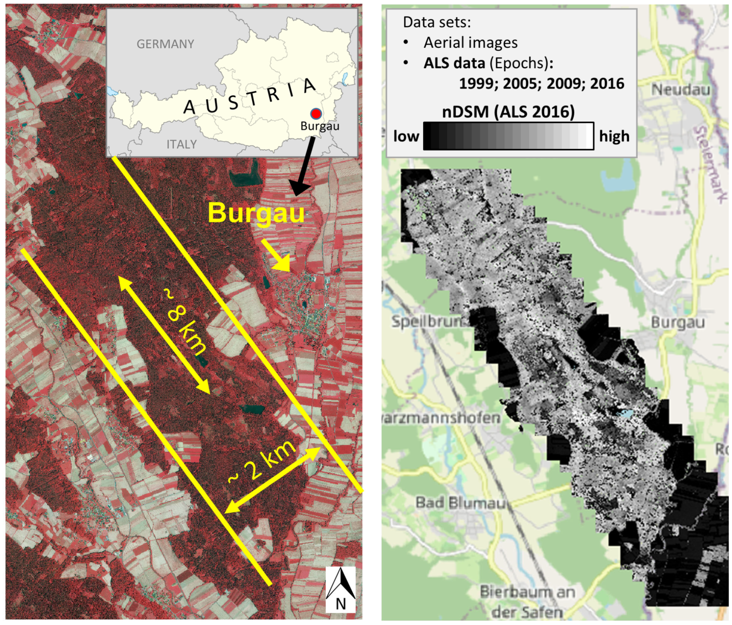
Figure 1. Study area and datasets NIR/color-infrared (CIR) (left) and ALS/nDSM (right).
Remotesensing 17 02847 g001
Figure 2. Aerial imagery used in this study: RGB (left) and near-infrared (NIR, (right)) images acquired in 2016, both with a spatial resolution of 9 cm.
Remotesensing 17 02847 g002
Figure 3. Tree height distributions for spruce, pine, and broadleaf trees in the training/validation dataset (left) and the independent test dataset (right).
Remotesensing 17 02847 g003
Figure 4. Field data acquisition: georeferencing of individual trees using a total station and recording of tree-specific parameters. The inset shows numbered ID tags used for tree identification in the field.
Remotesensing 17 02847 g004
Figure 5. General ALS data pre-processing workflow applied across all approaches (1D, 2D, 3D Voxel and PC). Trees are color coded by their height.
Remotesensing 17 02847 g005
Figure 6. Selection of optimal tree crown extraction radius for classification across four ALS datasets (2016, 2009, 2005, 1999) and four data representations: 1D vector, 2D raster, 3D voxel, and 3D point cloud. Results show mean accuracies from an early exploratory phase without hyperparameter tuning. A 3 m radius yielded the most consistent and robust performance across configurations. Y-axis values are omitted as the accuracies represent averages across radii, data types, and algorithms, rather than absolute performance metrics.
Remotesensing 17 02847 g006
Figure 7. Vertical point density profiles of normalized tree segments for broadleaf, pine, and spruce trees. Based on labeled reference data (see Section 2.3), the figure shows aggregated normalized point density (color scale) along normalized tree height, revealing characteristic differences in crown shape and vertical structure among tree types.
Remotesensing 17 02847 g007
Figure 8. Extraction of 1D features for tree type classification: (left)—Vertical Point Distribution (VPD), (middle)—mean of the normal component of the z-axis (Nz), and (right)—Tree Top Angle Statistics (TAS).
Remotesensing 17 02847 g008
Figure 9. Basic architecture of the neural network for tree type classification using 1D, 2D, or 3D data inputs.
Remotesensing 17 02847 g009
Figure 10. Transformer architecture for tree type classification based on 1D-features.
Remotesensing 17 02847 g010
Figure 11. Transformation of a point cloud into a 2D colored raster image (Colored Profile—CP).
Remotesensing 17 02847 g011
Figure 12. Visualization of the transformation process of unordered point cloud to ordered Point Density Voxels (left) and Binary Voxels (right) along with the corresponding DL architectures. * Layer parameters for TreeCNN_3D are provided in Figure 9.
Remotesensing 17 02847 g012
Figure 13. Tree type classification result based on ALS data. Trees labeled as “Not_classified” are those below 5 m in height and are not included in this visualisation.
Remotesensing 17 02847 g013
Figure 14. Comparison of classification results across various ML and DL models applied to different input data structures (1D vector, 2D raster, 3D voxel, and point cloud representations). The upper section shows overall OA per model, with vertical lines marking the range of class-specific accuracies. ML models are labeled with capital-letter acronyms, DL models with sequential numbers. The lower section visualizes the class-wise deviation from OA for spruce, pine, and broadleaf, effectively summarizing confusion matrix patterns using color-coded bars. For additional details on per-class performance, including confusion matrices, F1-scores, precision, and recall, see Appendix A.
Remotesensing 17 02847 g014
Figure 15. Feature importance analysis for 1D-data structure and ML classifiers.
Remotesensing 17 02847 g015
Figure 16. The probability distributions of the predictions spruce, pine, and broadleaf tree across selected models.
Remotesensing 17 02847 g016
Figure 17. Multi-View approach: rotation of a point cloud to generate 24 colored images per individual tree at 15° intervals (covering 0° to 360°).
Remotesensing 17 02847 g017
Figure 18. Effect of combining multiple Multi-View Profiles (MVPs) on classification accuracy across different 2D models. Results are based on 500 random combinations of 24 input images per tree to account for the influence of view order. The red shaded area indicates the standard deviation across simulations, reflecting the varying contribution of individual views.
Remotesensing 17 02847 g018
Table 1. Overview of traditional ML algorithms used in this study and the corresponding modified hyperparameters. All unspecified parameters remained at their default values as defined in scikit-learn (v1.2.2).
ML AlgorithmModified ParameterValue/Name
Random Forest (RF) [73,74] Number of trees:500
Split criterion:Entropy
Support Vector Classifier (SVC) [75]Regularization strength (C):100
Gamma:Auto (1/n_features)
Multilayer Perceptron Classifier (MLPC) [76]Hidden layers:2 (200 neurons each)
Optimizer:Lbfgs
Learning rate:Invscaling
Max. training epochs:1000
k-Nearest Neighbors (k-NN) [77]Number of neighbors (k):10
Logistic Regression (LR) [78]Extension:Multinomial
Regularization (C):0.2
Max. training epochs:2000
Linear Discriminant Analysis (LDA) [79]Optimizer:Lsqt
Shrinkage:Auto
Nearest Centroid/Min. Distance (NC) [80](Default parameters)---
Naive Bayes Classifier (NB) [81](Default parameters)---
Table 2. DNN, optimizer type, learning rate, and weight decay settings used for training the deep neural network models applied to the 2D raster-based tree classification. Unless stated otherwise, default parameters were used for all other hyperparameters.
Deep Neural Network (DNN)OptimizerLearning RateWeight Decay
Tree CNN_2D (see Section 3.2.3)RMSprop1 × 10−41 × 10−5
InceptionV3 [82]RMSprop1 × 10−41 × 10−5
Xception [83]RMSprop1 × 10−41 × 10−5
EfficientNet [84]RMSprop1 × 10−41 × 10−5
Vision Transformer (ViT) [85]AdamW1 × 10−31 × 10−4
Compact Convolutional Transformer (CCT) [86] AdamW1 × 10−31 × 10−4
Swin Transformer (SwinT) [87]AdamW with label smoothing of 0.11 × 10−31 × 10−4
Disclaimer/Publisher’s Note: The statements, opinions and data contained in all publications are solely those of the individual author(s) and contributor(s) and not of MDPI and/or the editor(s). MDPI and/or the editor(s) disclaim responsibility for any injury to people or property resulting from any ideas, methods, instructions or products referred to in the content.