Article

UAV-LiDAR-Based Study on AGB Response to Stand Structure and Its Estimation in Cunninghamia Lanceolata Plantations

1
Key Laboratory of Carbon Sequestration and Emission Reduction in Agriculture and Forestry of Zhejiang Province, Zhejiang A&F University, Hangzhou 311300, China
2
School of Environmental and Resources Science, Zhejiang A&F University, Hangzhou 311300, China
3
Jiande Forest Farm, Jiande 311604, China
*
Author to whom correspondence should be addressed.
Remote Sens. 2025, 17(16), 2842; https://doi.org/10.3390/rs17162842
Submission received: 4 June 2025 / Revised: 10 August 2025 / Accepted: 13 August 2025 / Published: 15 August 2025

Abstract

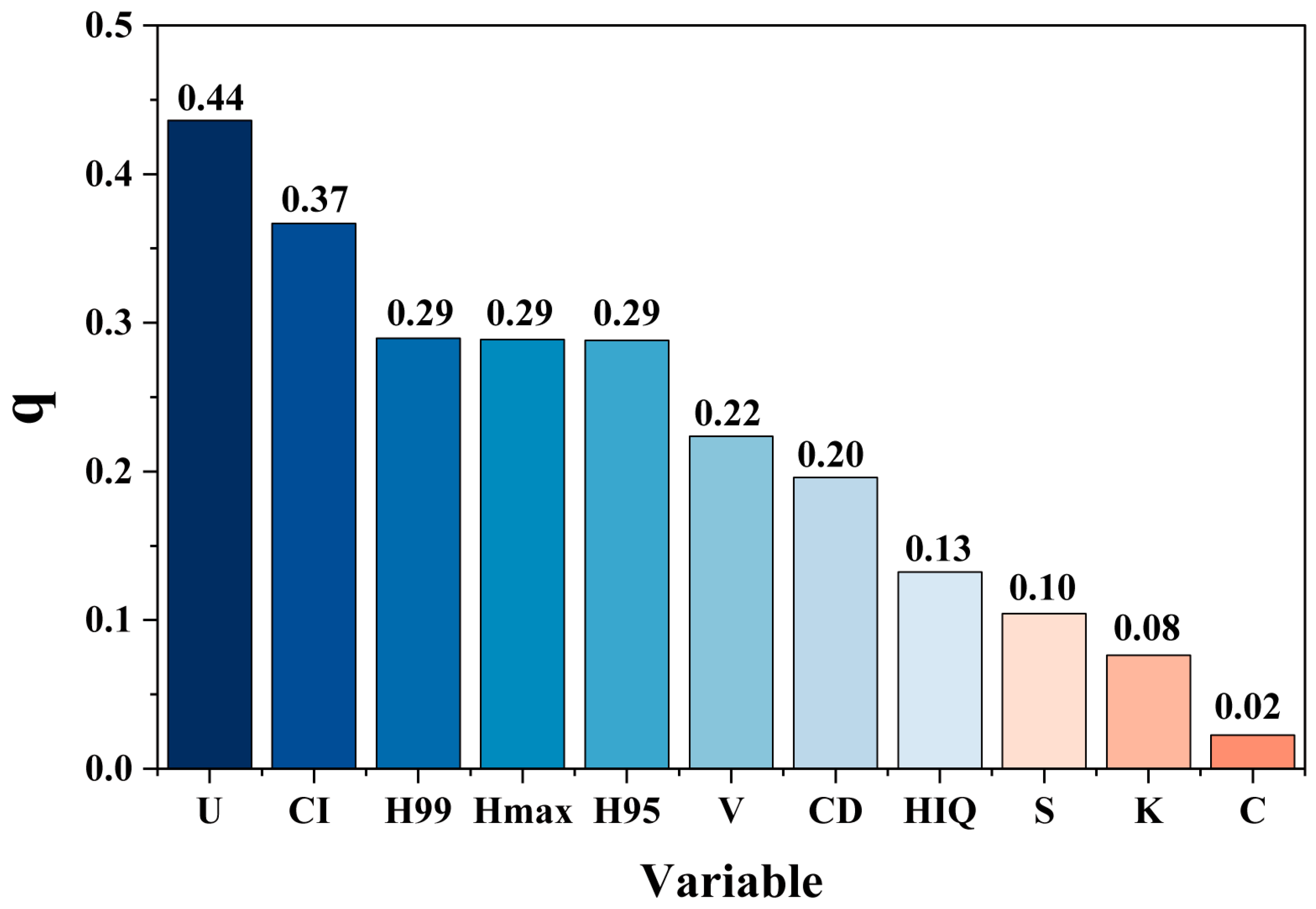
Forest spatial structure is of significant importance for studying forest biomass accumulation and management. However, above-ground biomass (AGB) estimation based on satellite remote sensing struggles to capture forest spatial structure information, which to some extent affects the accuracy of AGB estimation. To address this issue, this study focused on Chinese fir (Cunninghamia lanceolata) plantations in Zhejiang Province. Using UAV-LiDAR (unmanned aerial vehicle light detection and ranging) data and a seed-point-based individual tree segmentation algorithm, information on individual fir trees was obtained. Building on this foundation, structural parameters such as neighborhood comparison (U), crowding degree (C), uniform angle index (W), competition index (CI), and canopy openness (K) were calculated, and their distribution characteristics analyzed. Finally, these parameters were integrated with UAV-LiDAR point cloud features to build machine learning models, and a geographical detector was used to quantify their contribution to AGB estimation. The research findings indicate the following: (1) The studied stands exhibited a random spatial pattern, moderate competition, and sufficient growing space. (2) A significant correlation existed between the U and AGB (r > 0.6), followed by CI. The optimal stand structure for AGB accumulation was C = 0.25, U < 0.5, CI in (0, 0.8], and K > 0.3. (3) The four machine learning models constructed by coupling spatial structure with point cloud features all improved the accuracy of AGB estimation for the fir forest to some extent. Among them, the XGBoost model performed best, achieving a model accuracy (R2) of 0.92 and a relatively low error (RMSE = 14.02 kg). (4) Geographical detector analysis indicated that U and CI contributed most to AGB estimation, with q-values of 0.44 and 0.37, respectively.

1. Introduction

Forest spatial structure describes the spatial distribution and relationships among trees and their attributes [1,2,3,4], directly influencing light utilization efficiency, resource competition, and biomass accumulation. Key spatial structure indices, such as neighborhood comparison (U), crowding degree (C), uniform angular scale (W), aggregation index (R), competition index (CI), and openness (K), reflect both horizontal and vertical stand patterns and growth conditions [3,5,6,7,8]. The horizontal structure (e.g., tree distribution, density, crown overlap) and vertical structure (e.g., canopy stratification, tree height variation) not only determine forest growth potential but also significantly affect the spatial and temporal distribution of above-ground biomass (AGB) [9,10,11]. Therefore, understanding the role of spatial structure in AGB estimation can not only improve prediction accuracy but can also provide a scientific basis for biomass assessment and forest management optimization.
Traditional AGB estimation models often rely only on single variables like tree height and DBH. These models cannot fully capture how forest structure regulates photosynthesis and biomass formation. With the development of UAV-based LiDAR, it is now possible to represent forest spatial structure in three dimensions. This provides a solid foundation for studying the relationship between structure and AGB. Previous studies have shown that optimizing spatial structure is crucial for improving forest AGB and productivity [12,13]. Some researchers have explored how structural indices such as CI and C relate to AGB [13,14]. Others have identified stand structures with the highest management potential and ecological benefits [15]. In addition, some studies have examined canopy structure and its impact on AGB. Results show that canopy characteristics play an important role in boosting forest productivity [16]. For example, Xu et al. (2024) studied canopy heterogeneity and found that spatial structural diversity is closely linked to stand productivity [17].
Although previous studies have shown that forest spatial structure influences AGB accumulation to some extent [18,19], the underlying mechanisms involving multiple structural parameters remain unclear. In particular, strong interactions and coupling effects often exist among different spatial indices within a stand, and their combined impact on AGB has not been fully understood [20]. Moreover, the relative importance of various structural factors in contributing to AGB has yet to be quantified, limiting our understanding of the key drivers of carbon accumulation. Identifying the optimal range of spatial structure for AGB growth is also of practical significance, as it can inform silvicultural strategies and enhance forest carbon sink capacity [21]. Therefore, investigating the effects of spatial structure parameters on AGB and determining their optimal configurations can provide valuable scientific support for improving forest carbon sequestration and guiding ecological forest management.
Accurate acquisition of forest attributes and individual tree locations is essential for calculating spatial structure parameters. Most of the traditional methods for obtaining forest stand structure rely on manual field surveys, which are inefficient and costly [22]. As an active remote sensing technology, UAV-LiDAR (light detection and ranging) measures the distance between the sensor and objects by analyzing emitted and returned laser pulses [22,23]. This enables precise individual tree segmentation and retrieval of spatial location, tree height, crown width, and other key metrics [16,24,25,26]. Studies have shown that LiDAR provides high accuracy in estimating forest parameters such as tree height and volume. For instance, Fu et al. demonstrated high accuracy in LiDAR-derived tree height and biomass [27]; Cao et al. confirmed its reliability in predicting tree volume [28]; and Xu et al. found that LiDAR performs well in estimating DBH in complex stands [29]. These capabilities make LiDAR a powerful tool for analyzing the relationship between forest structure and ecological functions such as biomass and carbon storage [26,30,31].
Chinese fir (Cunninghamia lanceolata) is a key plantation species in southern China, playing an important role in carbon sequestration, timber production, and ecosystem services. Its stand structure is complex and highly sensitive to management practices, and structural information significantly influences the accuracy of above-ground biomass (AGB) estimation. This study takes Chinese fir plantations in Jiande Forest Farm, Zhejiang Province as the research object. First, individual tree attributes, such as diameter at breast height (DBH), tree height, crown width, spatial position, and point cloud features, were extracted using UAV-LiDAR and field plot data. Second, six spatial structure indices—neighborhood comparison (U), crowding degree (C), uniform angular scale (W), competition index (CI), and openness (K)—were calculated using the four nearest-neighbor method. Third, AGB was estimated by coupling spatial structure parameters and point cloud features in machine learning models. Finally, a geographic detector was used to assess the influence of spatial structure parameters on the spatial distribution of AGB. The main objectives of this study are to (1) analyze the effects of spatial structure parameters on AGB and identify optimal structural configurations; (2) evaluate how spatial structure influences the accuracy of AGB estimation models; and (3) identify the dominant structural factors driving the spatial variation of AGB.

2. Materials and Methods

2.1. Overview of the Study Area

As shown in Figure 1, the study area is located in Jiande Forest (119°56′E, 30°05′N~119°77′E, 30°10′N), Zhejiang Province. The study area is dominated by low hills, with the terrain high in the east and low in the west, and the elevation ranges from 100 to 500 m above sea level; it has a subtropical monsoon climate, with four distinct seasons and a mild and humid climate; the average annual temperature ranges from about 16 °C to 18 °C, with an extreme minimum of 6.6 °C and an extreme maximum of 30.4 °C. The annual precipitation ranges from 1400 mm to 1800 mm, and the highest precipitation season is summer. The main tree species in the study area is Chinese fir trees, with a forest cover of 77.92%.

2.2. Data Acquisition and Processing

2.2.1. UAV-LiDAR Data

The UAV-LiDAR point cloud data were acquired in August 2023 using a LiDAR system mounted on a DJI Matrice 350 hexacopter UAV. The system integrates a Velodyne Puck LITE laser scanner (sensor parameters are shown in Table 1), a GNSS receiver, and an IMU inertial navigation system, and the related equipment and composition are shown in Figure 1b. For data acquisition, the UAV flew at an altitude of 60 m, a flight speed of 8 m/s, a course spacing of 25 m, and a side-by-side overlap rate of 50% for data sampling, resulting in an average point cloud density of 400 points/m2.
After removing the noise from the original point cloud recorded by the LiDAR system [32], according to the improved progressive TIN densification (IPTD) encryption filtering algorithm proposed by Zhao et al. [33], the denoised LiDAR point cloud for ground point classification and the ground points therein were interpolated using triangulated irregular network (TIN) to obtain a digital elevation model (DEM) with a resolution of 0.5 m, and the DEM was subsequently used to normalized LiDAR data [28,34]. Meanwhile, in order to avoid the point cloud of low vegetation, such as weeds on the ground, from affecting the analysis of the mono-tree segmentation results, all laser points within 2 m from the ground point were removed [35,36].

2.2.2. Ground Survey Data

In August 2023, field measurements and positioning of individual trees were conducted in Jiande Forest Farm, Jiande City, Zhejiang Province, concurrently with the acquisition of UAV LiDAR data. A total of 1117 trees were surveyed, including Chinese fir and a few other species such as Masson pine, broadleaf trees, cypress, nanmu, and yew. Twenty 30 × 30 m sample plots were established within the study area, each surrounded by a 5 m buffer zone. Tree measurements included obtaining each tree’s position using Huace Intelligent RTK (accuracy better than 0.5 cm) and measuring the diameter at 1.3 m height with a diameter tape. Non-Chinese fir trees were removed during data processing. The statistical characteristics of the field survey data are presented in Table 2:

2.2.3. LiDAR Data Matching with Field Data

Field data were first filtered to exclude minor tree species as well as Chinese fir trees with a DBH less than 5 cm or a height less than 5 m. The filtered data were then further refined by removing outliers using the two-standard-deviation method. In this study, the individual tree coordinate data obtained from field surveys were treated as reference (ground truth) coordinates. The segmented individual trees derived from LiDAR data were then matched to the field data. Specifically, the coordinates from field surveys were matched with those from LiDAR-based individual tree segmentation, and field-measured DBH values were matched with tree height and crown width extracted from the LiDAR data. This process allowed the accurate identification of segmented trees and the retrieval of their corresponding attributes, including tree height, DBH, and crown width.

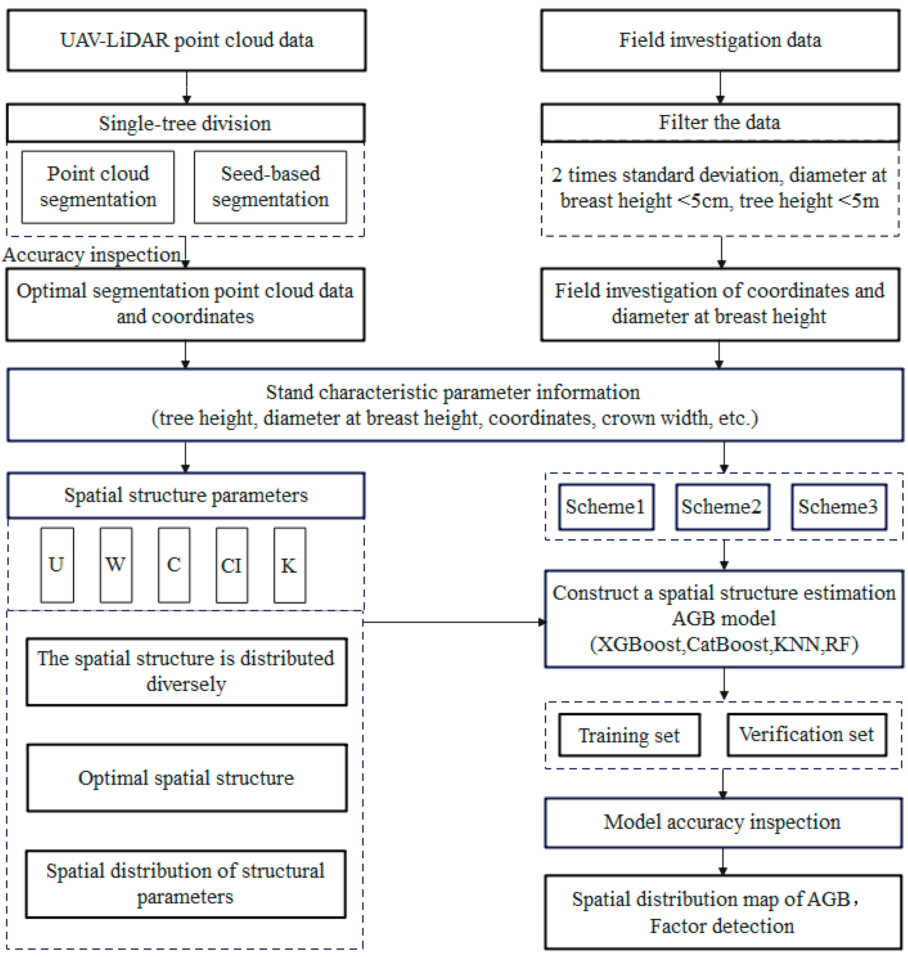
2.3. Technical Roadmap in the Paper

The flowchart of this study is shown in Figure 2. First, LiDAR data are preprocessed, individual trees are segmented, and point cloud feature variables are extracted. The coordinates and feature information of individual trees are then matched with field survey data. Second, spatial structural parameters are calculated, spatial distribution maps of forest structure are constructed, and forest stand spatial structural characteristics are analyzed. Next, AGB is calculated, and the relationship between forest spatial structure and AGB is examined. Finally, the accuracy of AGB estimation is compared across three schemes and four models, the spatial distribution of AGB is constructed, and factor detection is performed.

2.4. Segmentation and Evaluation of UAV Lidar Single Woods

Currently, UAV-LiDAR single-tree segmentation methods mainly include two approaches: segmentation based on canopy height models (CHMs) generated from LiDAR point cloud data [37,38], and segmentation based on point cloud distance thresholds [39,40]. The point cloud distance threshold-based segmentation method uses normalized point cloud data (often stored in LAS format) and distinguishes between different point clouds by analyzing spatial structure characteristics and applying a reasonable threshold to facilitate individual tree identification [41,42]. However, this method may encounter difficulties in extracting individual trees and reduced accuracy in densely forested stands [43]. Segmentation based on the point cloud CHM (canopy height model) effectively addresses these issues. CHM is created by classifying LiDAR point cloud data into ground and non-ground points, generating a digital terrain model (DTM) and a digital surface model (DSM) separately. The CHM is then obtained by subtracting the DTM from the DSM, producing raster data that clearly show the height distribution of the vegetation canopy top relative to the ground [44]. In contrast, CHM-based segmentation methods can effectively overcome these challenges. CHM-based methods include direct segmentation and seed-point-based individual tree segmentation. In this study, LiDAR360 software 5.2.2 was used to compare the accuracy of point cloud segmentation and seed-point-based segmentation. The optimal segmentation result was selected for extracting stand structure information. To evaluate the accuracy of individual tree segmentation, three metrics were adopted: crown detection rate (r), crown detection precision (p), and overall accuracy (F), as defined in Formulas (1)–(3) [22].
r = N t N t + N o
p = N t N t + N c
F = 2 r × p r + p
where N t is the number of correctly segmented singletons, N o is the number of missed singletons (the number of singletons that were actually present but not identified), and N c is the number of singletons that were segmented but were not present in the measured data.

2.5. Methods for Calculating Stand Spatial Structure Parameters

The stand spatial structure unit serves as the basis for calculating spatial structure parameters and evaluating the internal spatial characteristics of a forest stand. This study used the widely applied four-nearest-neighbor method to obtain stand spatial structure units. In this method, one tree is taken as the reference tree, and the four closest trees are considered its competitors, together forming a spatial structure unit [45,46]. To avoid errors caused by edge effects, a 5 m buffer zone was established along the edges of each sample plot. Trees located within this buffer zone were only considered as competitor trees for reference trees and were not used as reference trees themselves [36,47]. Based on the defined spatial structure units and buffer zones, and combined with the results of individual tree segmentation, five spatial structure parameters were calculated: neighborhood comparison (U), crowding degree (C), uniform angular scale (W), Hegyi competition index (CI), and openness index (K). The calculation methods are detailed in Table 3.
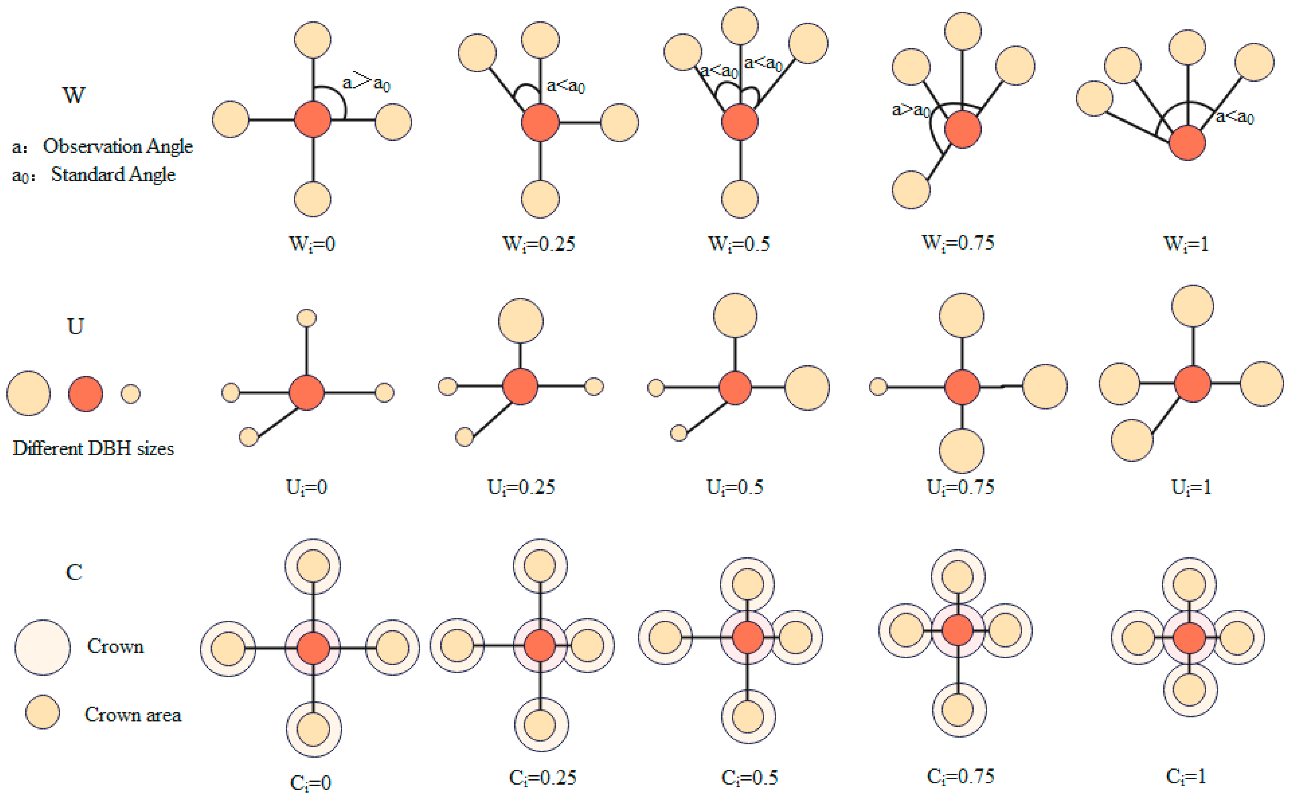
As shown in Figure 3, among the five spatial structure parameters, the neighborhood comparison (U), crowding degree (C), and uniform angular scale (W) can describe the spatial structure characteristics of forest stands from different levels and perspectives. Specifically, crowding degree (C) is calculated by taking each tree’s coordinates as the center and using the canopy area obtained from LiDAR data to form a circular area. According to the “telescope method” for interpreting forest spatial structure [50], the relationship between different combinations of structural parameters can be revealed through vertical projection-based dimensionality reduction and marginal probability distribution functions, thus providing a more comprehensive expression of the multivariate distribution characteristics. This study uses the correlation coefficient R to evaluate the relationship between structural parameters and AGB. The calculation formula is shown below:
R = 1     i = 1 n x ^ i x i 2 i = 1 n x i     x ¯ 2
In the formula, n is the number of samples, xi is the observed value of individual tree biomass, x ¯ is the mean of the observed biomass, and x ^ i is the predicted value of individual tree biomass.

2.6. Calculation of AGB for Single Wood in Ground Sample Plots

In this study, above-ground biomass (AGB) of individual Chinese fir trees was calculated based on an allometric growth equation, using tree height extracted from LiDAR-based individual tree segmentation and corresponding field-measured DBH values. The allometric growth equation for Chinese fir used in this study is as follows [51]:
W = 0.086 D 1.979 H 0.419
where D is the diameter at breast height of the stand, H is the height of the stand, and W is the biomass of a single stand.

2.7. Extraction of LiDAR-Derived Feature Variables

Feature variables derived from LiDAR data can be used to estimate forest structural parameters. Notably, point cloud features extracted from the first returns are significantly correlated with tree height, making them more suitable for estimating forest structure parameters [16,52,53]. To minimize the impact of ground vegetation and low-lying plants, all LiDAR points within 2 m of the ground were removed [35,36].
In this study, the LiDAR-derived feature variables include height metrics, density-based metrics, and canopy structure metrics. These encompass height percentiles and statistical measures of height. Density-based metrics (DB) describe the return density of the canopy and represent the proportion of point returns at specific height percentiles relative to the total number of points. Among the canopy structure metrics (CS), crown diameter is defined as the average of the east–west and north–south crown diameters; crown area (S) is calculated as the projected area of the crown point cloud using a 2D convex hull algorithm; and crown volume (V) is computed as the spatial volume occupied by the crown point cloud using a 3D convex hull algorithm. A detailed description of the point cloud feature variables is provided in Table 4 below.

2.8. AGB Estimation Model Schemes and Evaluation

In this study, based on the calculated stand spatial structure parameters and the extracted LiDAR-derived feature variables, four models—XGBoost, CatBoost, KNN, and random forest (RF)—were employed to construct AGB estimation models, and their accuracies were compared. To investigate the capability and applicability of stand structural parameters in estimating AGB, three modeling schemes were designed: scheme 1 includes only spatial structure parameters and is referred to as “Scheme 1”; scheme 2 uses only LiDAR-derived feature variables and is referred to as “Scheme 2”; scheme 3 combines both structure parameters and LiDAR features and is referred to as “Scheme 3”.
XGBoost, or extreme gradient boosting, is a boosting-based ensemble learning algorithm that enhances weak learners into strong learners [59,60]. It continuously adds CART (classification and regression tree) decision trees to the model, using each new tree to fit the residuals of previous predictions. The final prediction is obtained by summing the outputs of all trees [61]. XGBoost has demonstrated excellent predictive performance in biomass estimation and can achieve more accurate predictions of AGB [62]. CatBoost is a machine learning algorithm based on gradient boosting, known for its ability to reduce prediction bias and prevent overfitting [63]. The K-nearest neighbors (KNN) algorithm is a non-parametric method that predicts the class or value of a target sample based on the K nearest samples in the feature space [64]. The random forest (RF) model is a commonly used machine learning model. It is a non-parametric modeling method based on an improved version of decision trees. The model uses the bootstrap sampling method, which involves randomly sampling with replacement from the original dataset to select n samples for constructing multiple decision trees, which are then used for prediction. The advantages of the random forest model include ease of implementation, strong noise resistance, and fast computation speed [65].
During the modeling process, the dataset was split into training and testing sets in an 8:2 ratio, with 80% of the samples used for training and the remaining 20% as independent test samples to validate AGB estimation accuracy. Model performance was evaluated using the coefficient of determination (R2), root mean square error (RMSE), and relative root mean square error (rRMSE). A higher R2 and lower RMSE and rRMSE indicate better model performance. The formulas for calculating R2, RMSE, and rRMSE are as follows:
R 2 = 1     i = 1 n x ^ i     x i 2 i = 1 n x i     x ¯ i 2
R M S E = 1 n i = 1 n ( x i x ^ i ) 2
r R M S E = R M S E x ¯ × 100 %
where n is the number of samples, x i is the measured value of single tree biomass, x ¯ is the mean value of single tree biomass, and x ^ i is the predicted value of single tree biomass.

2.9. Geographical Detector Factor Analysis

The geographical detector model OPGD (optimal parameters-based geographical detector model) is an improved method developed from the traditional geographical detector model. It systematically explores the optimal combination of parameters such as spatial scale, spatial data discretization methods, and the number of spatial partitions, aiming to enhance the model’s applicability and accuracy in detecting spatial heterogeneity [66]. In this study, the factor detector component of the OPGD model is primarily used to analyze the driving forces of influencing factors. The factor detector evaluates the explanatory power of a single factor on the spatial heterogeneity of the dependent variable, thereby determining which factors play significant roles in the spatial distribution of geographical phenomena. This method provides an effective approach for quantifying the importance of factors and helps identify the key elements driving changes in geographical processes. In this study, the importance of each factor is quantified using the q-value, which ranges from 0 to 1. A higher q-value indicates a stronger explanatory power of the factor. The calculation formula for the q-value is as follows:
q = 1     h = 1 L N h σ h 2 N σ 2
In the formula, q represents the explanatory power of each variable on AGB variation—the larger the value, the stronger the explanatory ability of the independent variable on AGB. h is the number of categories (or strata) of the independent variable; Nₕ and N are the number of samples in category h and the total number of samples in the study area, respectively; σh2 and σ2 are the variance of the dependent variable within category h and the total variance of the dependent variable, respectively.

3. Results

3.1. Individual Tree Segmentation Based on UAV-LiDAR

The individual tree segmentation accuracy of Chinese fir plantations based on UAV-LiDAR is shown in Table 5. As can be seen from Table 5, the point cloud segmentation method correctly segmented 430 trees, with 123 trees missed and 91 trees incorrectly segmented. The detection rate (r) for the entire plot was 78%, the precision (p) was 82%, and the overall accuracy (F) was 80%. In contrast, the seed point-based segmentation method correctly segmented 521 trees, with 64 missed and 59 incorrectly segmented, achieving a detection rate of 89%, a precision of 90%, and an overall accuracy of 89%. These results indicate that the seed point-based method provides higher accuracy in individual tree segmentation. Figure 4a shows the segmentation results of Chinese fir plantations based on UAV-LiDAR. Figure 4b,c compare the local segmentation performance of the seed point-based and point cloud-based methods. It is evident that the point cloud segmentation method exhibits greater errors in delineating individual trees. Therefore, the seed point-based method, due to its higher accuracy in segmenting Chinese fir trees, was adopted in this study for individual tree segmentation and structural information extraction.

3.2. Multivariate Spatial Distribution Characteristics of Chinese Fir Forest Structure

Based on the individual tree segmentation, this study calculated and analyzed the spatial structural parameters of Chinese fir plantations using the formulas and methods as shown in Table 3 and Figure 2.

3.2.1. Univariate Distribution

The univariate distributions of Chinese fir C, W, U, and frequency are shown in Figure 5a. The cumulative frequency is highest at a density of C = 0.5, with a relative frequency of 25%, indicating that most tree crowns in the forest overlap with the crowns of at least two neighboring trees. The frequency gradually decreases on both sides of 0.5, showing an overall trend of a normal distribution. The frequency distributions of density C at 0.25 and 0.75 are 20% and 21%, respectively, indicating that a certain number of tree crowns are in sparse to medium–high density conditions. The angular scale W has the highest cumulative frequency at the level W = 0.5, with a relative frequency of 45%. The frequency decreases gradually on both sides of W = 0.5, with the least frequency at W = 1. This overall normal distribution of angular scale frequency indicates that most trees are randomly distributed. The diameter size ratio U is evenly distributed across all levels, with an average frequency around 20% for each level, suggesting relatively low competition pressure among trees and a balanced growth status.
The frequency distributions of the Chinese fir CI and K are shown in Figure 5b. It can be seen that the relative frequency distributions of both CI and K generally follow a normal distribution. The CI frequencies are mainly concentrated between (0.2, 0.8] and (0.8, 1.4]. A higher competition index indicates greater competitive pressure on the subject tree from neighboring trees. The competition pressure among Chinese firs in the plot is moderate to low, which is beneficial for the overall healthy growth of the stand. The frequency distribution of K is lower at the extreme ends and mainly concentrated in the intervals (0.2, 0.3] and (0.3, 0.4], with the relative frequency in the (0.2, 0.3] interval reaching 50%. This suggests that most trees in the stand have ample growing space.

3.2.2. Bivariate Distribution

The bivariate distributions of three structural parameters of Chinese fir—W, C, and U—are shown in Figure 6. Figure 6a presents the combination of W and U. It can be observed that when the W is fixed, the U is distributed relatively evenly across all levels, with an average frequency of 20%. Trees that are both randomly distributed and in a moderate growth state (W = 0.5, U = 0.5) account for 10%, indicating balanced tree growth. Figure 6b shows the combination of W and C. When W is at a certain level, the cumulative frequencies of C are highest at C = 0.5 and C = 0.75, with 25% and 21%, respectively. Among them, trees that are randomly distributed and at moderate density (W = 0.5, C = 0.5) account for 11%. Figure 6c illustrates the combination of U and C. It can be seen that trees in a moderate growth state with medium density canopy (U = 0.5, C = 0.5) account for 6%. More than half of the trees have a C greater than 0.5, indicating that the Chinese fir plantations are generally at medium to high density levels.

3.2.3. Trivariate Distribution

The combination of three structural parameters of Chinese fir—W, C, and U—constitutes the trivariate distribution, as shown in Figure 7. From Figure 7, it can be seen that when the U is fixed, the frequency distribution of the W is highest at W = 0.5. Trees in a moderate growth state and medium density (W = 0.5, U = 0.5, C = 0.5) account for 4%. Cases where tree crowns overlap with those of three to four surrounding trees (C = 0.75, C = 1) account for 17%, indicating that crown connectivity with neighboring trees is common. The W follows an overall normal distribution, with W = 0 and W = 1 together accounting for 4%. The diameter size ratio U is evenly distributed across levels. Among them, trees that are very evenly distributed, dominant in growth, and at high density (W = 0, U = 0, C = 1) account for only 1%, while trees that are extremely unevenly distributed, dominant in growth, and have sparse crowns (W = 1, U = 0, C = 0) also account for only 1%. When W and U are fixed, the C mainly concentrates around C = 0.5. This further indicates that most trees in the Chinese fir plantations are randomly distributed, with moderate growth, and crowns exhibiting medium density. Trees showing extremely unreasonable distributions across all three parameters account for a very small proportion.

3.3. Correlation Analysis Between Stand Structure and AGB

Based on a thorough understanding of the stand’s spatial structure, the correlation analysis between structural parameters and AGB is shown in Figure 8. As shown in Figure 8a, there is a significant negative correlation between U and AGB, with a correlation coefficient R of −0.66 (p ≤ 0.001). The smaller the U, the fewer the neighboring trees with a larger diameter than the reference tree [67]. In other words, when U is smaller, the neighboring trees around the target tree have smaller diameters, resulting in greater AGB for the target tree. According to the multivariate distribution, the U of Chinese fir mainly concentrates around levels 0.5 and 0.75, indicating that smaller U in the study area are more favorable for AGB accumulation. Figure 8b shows a weak negative correlation between C and AGB. Although the correlation is low, it still suggests that a less dense environment is more conducive to biomass growth. There is no significant correlation between W and AGB (Figure 8c). Figure 8d,e indicate that both CI and K have significant correlations with AGB. Specifically, CI and AGB show a significant negative correlation with a coefficient of −0.61 (Figure 8d), implying that lower competition pressure on trees favors biomass growth. The correlation coefficient between K and AGB is 0.26 (Figure 8e), indicating that more available growing space within the stand benefits biomass increase.
In summary, the spatial structure of Chinese fir, especially U, CI, and K, shows significant correlations with AGB. When tree crowns overlap less with neighboring competitors and trees have sufficient growing space with reduced competition, the trees can accumulate more biomass under better growth conditions.
This study, based on the multivariate distribution of structural parameters shown in Figure 2, randomly combined the levels of four spatial structure parameters—U, C, CI, and K—and calculated the average AGB of single Chinese fir trees under different combinations to further analyze the influence of spatial structure on AGB, as shown in Figure 9. The points with different colors in the figure represent different CI-K level combinations. Analysis of Figure 9 reveals that the AGB of Chinese fir decreases as C and U levels increase, reaching its highest value when C = 0.25 and U < 0.5. Meanwhile, when CI is in the range (0, 0.8] and K is in the range (0.3, ∞), the AGB is at its maximum. Therefore, the favorable spatial structure for AGB accumulation in Chinese fir plantations is characterized by C = 0.25, U < 0.5, CI in (0, 0.8], and K in (0.3, ∞).
Figure 9 also employs an importance analysis method to further evaluate the influence of U, C, CI, and K on Chinese fir AGB. It shows that U accounts for 63.13% of the importance, having the greatest effect on biomass. CI ranks second with 19.16%, while K and C contribute relatively less, at 10.10% and 7.62%, respectively. This indicates that increasing openness, reducing competition among trees, and cultivating large-diameter trees are key management practices to optimize Chinese fir plantation structure and enhance AGB.

3.4. Construction of AGB Estimation Model and Accuracy Comparison

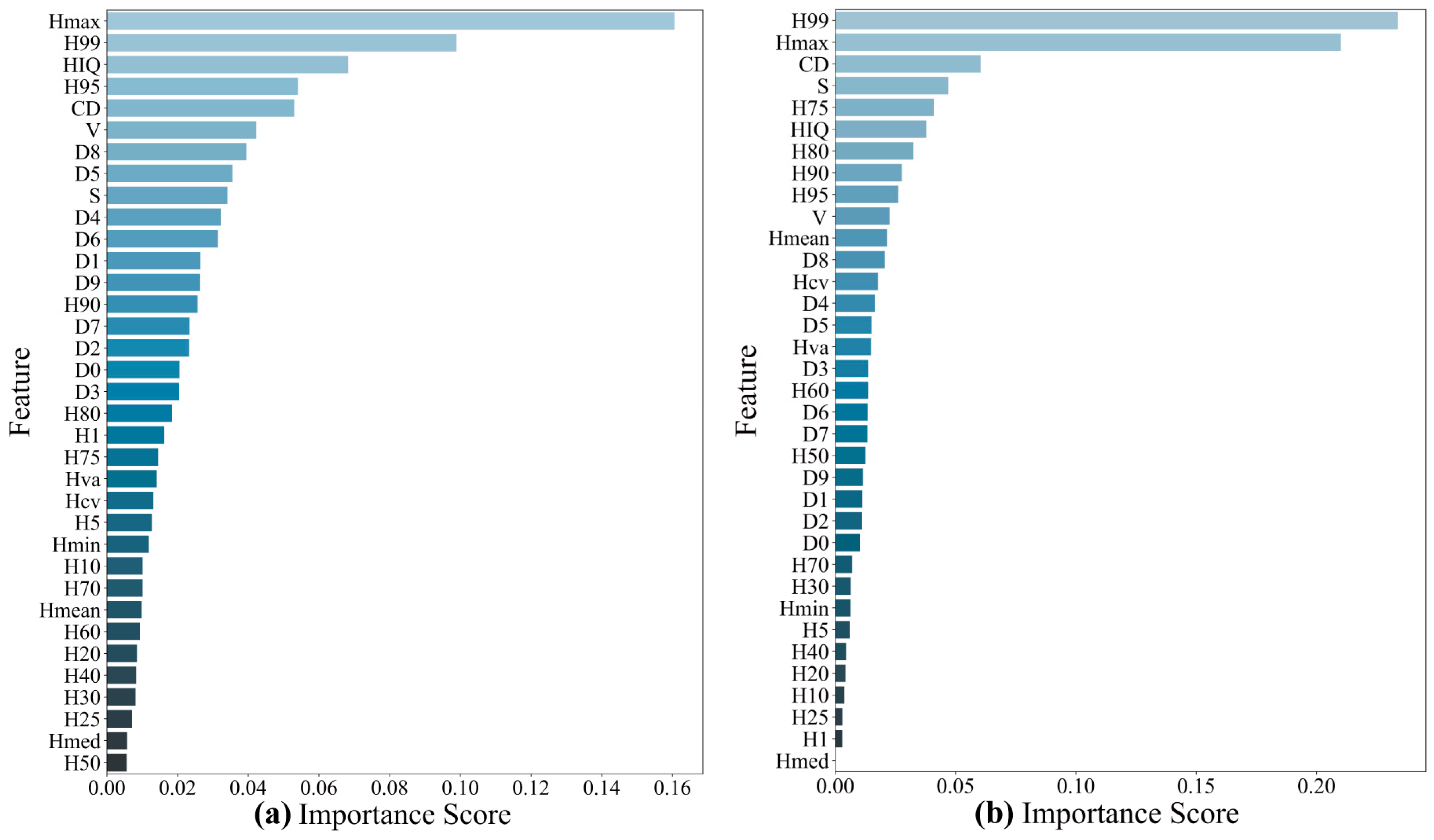
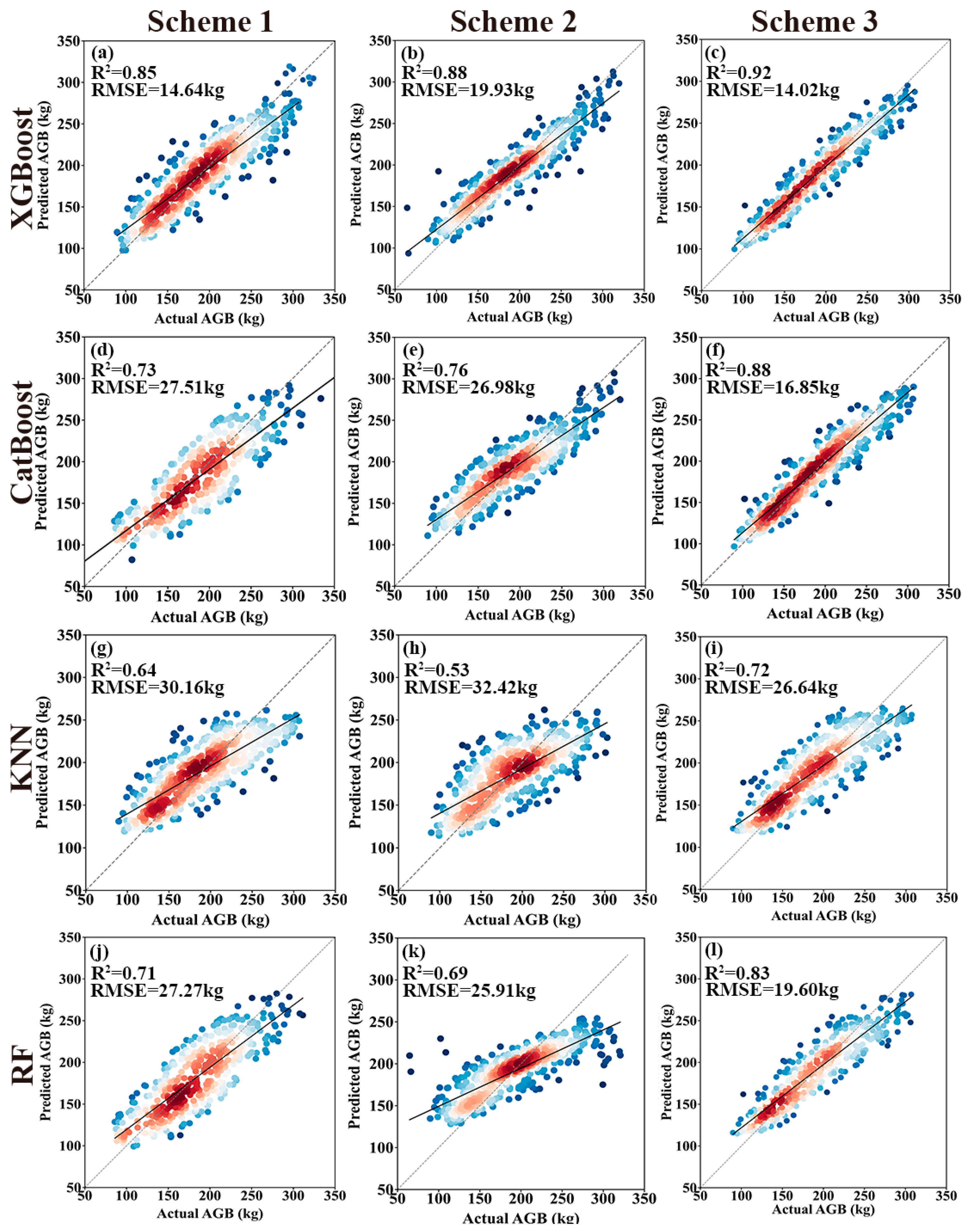
This study conducts an importance analysis of the feature variables of single-tree point clouds obtained based on unmanned aerial vehicle lidar. Figure 10 is a bar chart of feature importance based on the RF model and the XGBoost model. As can be seen from Figure 10, the top ten variables in terms of importance for both models include Hmax, H99, H95, HIQ, CD, S, and V. Therefore, based on the analysis of their importance, these seven characteristic variables were selected. Four models, namely XGBoost, CatBoost, KNN, and RF, were respectively used to estimate AGB modeling for the characteristic variables of Scheme 1, Scheme 2, and Scheme 3. The total accuracy results are shown in Figure 11. As can be seen from the figure, the XGBoost model has the highest accuracy in estimating AGB among the three schemes. It can be seen from Figure 11a,b,d,e,g,h,j,k that the accuracy results of estimating AGB by Scheme 1 and Scheme 2 in the four models are comparable, and when based on the KNN and RF models, the accuracy of Scheme 1 is higher than that of Scheme 2. Scheme 3 performed the best among the four models. When using the XGBoost model, the accuracy R2 was 0.92 (Figure 11c), which was 8.24% higher than that of Scheme 1 R2, with RMSE reduced by 0.62 kg, and 4.55% higher than that of Scheme 2 R2, with RMSE reduced by 5.91 kg. When using the CatBoost model, the accuracy R2 = 0.88 (Figure 11f), which is 20.55% higher than that in Scheme 1′s R2, and the RMSE decreases by 10.66 kg. Compared with Scheme 2′s R2, it is 15.79 higher, and the RMSE decreases by 10.13 kg. When using the KNN model, the accuracy R2 = 0.72 (Figure 11i), which is 12.5% higher than that in Scheme 1’s R2, and the RMSE decreases by 3.52 kg. Compared with Scheme 2’s R2, it is 35.85% higher, and the RMSE decreases by 5.78 kg. When using the RF model, the accuracy R2 = 0.83 (Figure 11l), which is 16.9% higher than that in Scheme 1’s R2, with RMSE decreasing by 7.67 kg, and 20.29% higher than that in Scheme 2’s R2, with RMSE decreasing by 6.31 kg.

3.5. Spatial Distribution of AGB in Chinese Fir

The spatial distribution of structural parameters in the study area is shown in Figure 12. It can be observed that the spatial distribution of U is relatively uniform across the area. The parameter C is mainly concentrated in three levels: 0.5, 0.75, and 1. The CI is primarily distributed within the range of (0.3, 0.8], while the K is mostly concentrated in the range of (0.4, ∞). The tree AGB ranges from 86.9 kg to 396.1 kg, with an average AGB of 197.4 kg. It can be concluded that areas with lower U and C levels and lower K values tend to have higher AGB. Overall, the spatial distribution of structural parameters aligns with the optimal structure identified in Section 3.3.
The above analysis reveals that, except for the W, which shows no significant correlation with the AGB of Chinese fir, the U, C, CI, and K all exhibit a clear correlation with AGB. Among all the models, the XGBoost model performs the best. Therefore, we selected structural parameter schemes 1, 2, and 3 as input variables and used the XGBoost machine learning algorithm to build AGB prediction models and analyze AGB spatial distribution in the study area. As shown in Figure 13, Figure 14 and Figure 15, AGB estimates under schemes 1, 2, and 3 are most frequently distributed within the 150–250 kg range, accounting for over 35% of the total. Scheme 1 achieved an estimation accuracy of R2 = 0.85 and RMSE = 14.64 kg (Figure 13b). The spatial and frequency distributions are shown in Figure 13a,c,d. Scheme 2 yielded a slightly higher accuracy with R2 = 0.88 and RMSE = 19.93 kg (Figure 14b), though its training and test datasets showed fewer samples in the AGB < 150 kg and AGB > 300 kg ranges compared to scheme 1. Scheme 3 produced the highest accuracy, with R2 = 0.92 and the lowest RMSE of 14.02 kg (Figure 15b). Moreover, it had a greater number of samples with AGB > 300 kg in both the training and test sets compared to schemes 1 and 2.
Overall, scheme 1′s accuracy is only slightly lower than schemes 2 and 3, and the integration of point cloud features with structural parameters has led to noticeable improvement in model performance. Scheme 3′s spatial AGB distribution (Figure 15a) also closely aligns with that of Scheme 1, showing minimal distribution error.
Furthermore, the factor detector from the geographic detector framework was employed to assess the explanatory power of individual factors on AGB. Figure 16 presents the results of each factor’s independent influence on AGB in scheme 3. A higher q-value indicates a stronger explanatory power of the independent variable on AGB. As shown in the figure, among the spatial structural parameters, U exhibits the highest discriminative power for AGB prediction (q = 0.44, p < 0.001). The CI (q = 0.37), as well as the high-order percentile parameters H99 (q = 0.29), Hmax (q = 0.29), and H95 (q = 0.29), also demonstrate relatively high explanatory power, all of which are statistically significant at the p < 0.001 level. This indicates that spatial structural parameters play a more critical role in predicting AGB.
In conclusion, the AGB estimation model constructed using stand structural parameters directly extracted from UAV LiDAR data can accurately estimate the AGB and its spatial distribution for Chinese fir forests.

4. Discussion

LiDAR technology has been widely applied in studies of forest structure and ecological functions due to its ability to capture high-precision, tree-level structural information [68]. In this study, UAV-LiDAR point cloud data were used to compare two individual tree segmentation methods: seed point-based and point cloud-based approaches. Many studies have found that point cloud-based segmentation offers higher accuracy and broader applicability. For example, Li et al. (2018) tested several algorithms in subtropical plantations in southeastern China and found that point cloud-based methods performed best in complex stands [37]. However, segmentation accuracy is affected by various factors, such as tree species, stand structure, canopy cover, and algorithm design [69]. In our study, the seed point-based method showed better accuracy, with lower omission and commission rates. This result differs from that of Li et al. [37]. One possible reason is the site conditions. Our study area has medium to high stand density, dense understory vegetation, and complex terrain. These factors can cause overlapping canopy heights during point cloud normalization, making it difficult to detect crown boundaries. In contrast, the seed point-based method relies on local maxima detection, which makes it more robust under conditions of canopy overlap and terrain variation.
Building on this, the study further extracted spatial structure parameters of Chinese fir plantations. Univariate distribution analysis showed that the proportions of trees with “highly uniform” or “highly clustered” angular scale (W) were low, indicating that the stand tended toward a moderate structural state under management disturbance [70,71]. Results from competition index (CI), stand density (C), and openness (K) revealed moderate overall density but significant crown overlap. This may reduce light availability in the understory, hinder vegetation regeneration, and negatively affect sustainable forest management. However, univariate indicators reflect only a single aspect of structure and cannot fully assess overall spatial rationality [49]. Therefore, this study introduced multivariate distribution analysis, including bivariate and trivariate structural distributions, to evaluate tree isolation, crowding, and spatial coherence [72,73]. The results showed that only 9% and 4% of trees had structurally unreasonable positions under bivariate and trivariate analysis, respectively, suggesting good overall structure with some room for local improvement. Based on this, we recommend applying structure-oriented thinning. By removing individuals with highly unreasonable spatial positions, the stand layout can be optimized, thereby improving AGB in Chinese fir plantations.
To quantify the relationship between spatial structure parameters and AGB, this study analyzed the correlations between key structural indices and AGB. The results showed that dominance index (U) and competition index (CI) were significantly negatively correlated with AGB (U: r = –0.66; CI: r = –0.61), while openness (K) was positively correlated (r = 0.26). This suggests that lower competition pressure and greater spatial isolation promote tree growth and AGB accumulation. Stand density (C) showed a weak negative correlation with AGB (r = –0.10), which differs from the findings of Khan et al. [74]. This discrepancy may be due to the moderate stand density in the study area, which does not reach a threshold that imposes strong competition. These results align with the trade-off relationship between maximum DBH and relative growth rate reported by Protazio et al. [75] and are consistent with studies by Tang et al. [13] and Qiu et al. [76], which found that low competition intensity enhances biomass accumulation. The optimal spatial structure for AGB (C = 0.25, U < 0.5, CI ∈ (0, 0.8], K > 0.3) indicates that a moderately sparse, low-competition, and open stand structure is most favorable for carbon accumulation. This finding highlights the importance of spatial structure regulation in forest management and provides a reference for structural optimization [10,77].
To further evaluate the impact of spatial structure on improving AGB estimation accuracy, this study designed three modeling schemes: using only spatial structure parameters (scheme 1), only point cloud features (scheme 2), and a combination of both (scheme 3). Four algorithms—XGBoost, CatBoost, KNN, and RF—were applied. Results showed that XGBoost consistently outperformed the others, with the highest accuracy and lowest RMSE, demonstrating its strength in handling nonlinear relationships and complex variables [78,79]. Scheme 3 outperformed both scheme 1 and scheme 2, with predictions closer to observed values and fewer outliers, indicating that integrating spatial structure with point cloud features significantly enhances the robustness and adaptability of AGB estimation [44].
To further explore the relative contribution of each variable to AGB estimation, this study applied geographic detector analysis. Results showed that spatial structure parameters (especially size ratio (U) and competition index (CI)) contributed more to AGB than point cloud features. This supports the findings of Dong et al. [10]., who reported that spatial structure features are more sensitive to biomass variation than traditional LiDAR height metrics, such as CHM. The study also found that AGB tends to accumulate more easily when stands are randomly distributed, trees are in dominant or intermediate positions, crown overlap is moderate, spacing between individuals is reasonable, and competition intensity is balanced [80].
In summary, forest spatial structure has a significant impact on AGB, with structural parameters—especially size ratio (U) and competition index (CI)—providing more accurate explanations of AGB variation. Integrating point cloud features with spatial structure data improves estimation accuracy and shows strong practical potential. This study deepens the understanding of the spatial structure–AGB relationship and offers a feasible approach to enhancing carbon storage, optimizing forest structure, and promoting sustainable forest management. Future research should expand to include diverse forest types, landforms, and climate zones, aiming to develop more adaptable structure–function models for high-precision AGB monitoring and sustainable management guided by spatial structure.

5. Conclusions

This study, based on UAV LiDAR and field survey data, analyzed the effects of spatial structure parameters (including size ratio (U), density (C), angle index (W), competition index (CI), and openness (K)) on the AGB of Chinese fir plantations. Results showed that U had the greatest impact on AGB, followed by CI, both showing negative correlations. The optimal spatial structure for AGB accumulation was identified as U < 0.5, CI between 0 and 0.8, C = 0.25, and K > 0.3. Models combining spatial structure and point cloud features achieved significantly higher AGB estimation accuracy than using either alone, with improvements ranging from 4.55% to 35.85%. Among all variables, U had the strongest explanatory power for AGB according to the geographic detector analysis, followed by CI. This highlights the dominant role of individual tree growth traits in AGB formation. The findings suggest that enhancing AGB prediction and forest carbon management should prioritize adjusting diameter structure, supported by optimizing competition patterns to achieve greater carbon gain.

Author Contributions

Y.C., writing—original draft, validation, methodology, formal analysis, data curation; Y.Z., data curation; J.X. (Jiuen Xu), data curation; Q.F., investigation; J.X. (Jie Xuan), data curation; L.H., data curation; X.L., funding acquisition, writing—review and editing; F.M., formal analysis, writing—review and editing; Y.S., data curation; H.D., writing—review and editing, funding acquisition, supervision, project administration, conceptualization. All authors have read and agreed to the published version of the manuscript.

Funding

This research was supported by the Leading Goose Project of Science Technology Department of Zhejiang Province (No. 2023C02035) and the National Natural Science Foundation (No. 32171785, 32201553). We further thank all editors and anonymous reviewers for spending their time working on the manuscript.

Data Availability Statement

The original contributions presented in the study are included in the article, further inquiries can be directed to the corresponding author.

Conflicts of Interest

The authors declare that they have no known competing financial interests or personal relationships that could have appeared to influence the work reported in this paper.

References

  1. Tang, M. Advances in study of forest spatial structure. Sci. Silvae Sin. 2010, 46, 117–122. [Google Scholar]
  2. Tang, M.; Tang, S.; Lei, X.; Li, X. Study on spatial structure optimizing model of stand selection cutting. Sci. Silvae Sin. 2004, 40, 25–31. [Google Scholar]
  3. Huang, T.; Ou, G.; Xu, H.; Zhang, X.; Wu, Y.; Liu, Z.; Zou, F.; Zhang, C.; Xu, C. Comparing Algorithms for Estimation of Aboveground Biomass in Pinus yunnanensis. Forests 2023, 14, 1742. [Google Scholar] [CrossRef]
  4. Chen, Y.; Yang, H.; Ma, S.; Ren, M. Spatial structure diversity of semi-natural and plantation stands of larix gmelini in Changbai Mountains, northeastern China. J. Beijing For. Univ. 2015, 37, 48–58. [Google Scholar]
  5. Clark, P.J.; Evans, F.C. Distance to nearest neighbor as a measure of spatial relationships in populations. Ecology 1954, 35, 445–453. [Google Scholar] [CrossRef]
  6. Heggi, F. A simulation models for managing jack pine stands, Growth models for tree and stand simulation. For. Res. 1974, 1, 74–90. [Google Scholar]
  7. Li, Y.; Hui, G.; Wang, H.; Zhang, G.; Ye, S. Selection priority for harvested trees according to stand structural indices. iForest-Biogeosci. For. 2017, 10, 561–566. [Google Scholar] [CrossRef]
  8. Aguirre, O.; Hui, G.; von Gadow, K.; Jiménez, J. An analysis of spatial forest structure using neighbourhood-based variables. For. Ecol. Manag. 2003, 183, 137–145. [Google Scholar] [CrossRef]
  9. Zhao, C.; Wang, J.; Zhou, G.; Yu, L.; Gong, X.; Meng, J. Logging Simulation of Natural Mixed Forest in Jinpen Mountain Based on Optimization of Spatial Structure. J. Southwest For. Univ. 2022, 42, 126–133. [Google Scholar]
  10. Dong, L.; Bettinger, P.; Liu, Z. Optimizing neighborhood-based stand spatial structure: Four cases of boreal forests. For. Ecol. Manag. 2022, 506, 119965. [Google Scholar] [CrossRef]
  11. Hui, G.; Hu, Y. Measuring Species Spatial Isolation in Mixed Forests. For. Res. 2001, 14, 23–27. [Google Scholar]
  12. Chen, A.; Xu, C.; Zhang, M.; Guo, J.; Xing, X.; Yang, D.; Xu, B.; Yang, X. Cross-scale mapping of above-ground biomass and shrub dominance by integrating UAV and satellite data in temperate grassland. Remote Sens. Environ. 2024, 304, 114024. [Google Scholar] [CrossRef]
  13. Tang, M.; Xu, W.; Chen, Y.; Deng, Y.; Zhao, M. Relationship between spatial structure and biomass of a close-to-nature Phyllostachys edulis stand in Tianmu Mountain. Sci. Silvae Sin. 2011, 47, 1–6. [Google Scholar]
  14. Li, Q.; Liu, Z.; Jin, G. Impacts of stand density on tree crown structure and biomass: A global meta-analysis. Agric. For. Meteorol. 2022, 326, 109181. [Google Scholar] [CrossRef]
  15. Yang, S.; Mao, K.; Yang, H.; Wang, Y.; Feng, Q.; Wang, S.; Miao, N. Stand characteristics and ecological benefits of Chinese Fir, Chinese Cedar, and mixed plantations in the mountainous areas of the Sichuan Basin. For. Ecol. Manag. 2023, 544, 121168. [Google Scholar] [CrossRef]
  16. Cao, L.; Coops, N.C.; Sun, Y.; Ruan, H.; Wang, G.; Dai, J.; She, G. Estimating canopy structure and biomass in bamboo forests using airborne LiDAR data. ISPRS J. Photogramm. Remote Sens. 2019, 148, 114–129. [Google Scholar] [CrossRef]
  17. Xu, Y.; Chen, H.Y.; Qiao, X.; Zhang, Y.; Jiang, M. The control of external and internal canopy structural heterogeneity on diversity and productivity relationship in a subtropical forest. For. Ecosyst. 2024, 11, 100246. [Google Scholar] [CrossRef]
  18. Liu, L.; Zeng, F.; Song, T.; Wang, K.; Du, H. Stand structure and abiotic factors modulate karst forest biomass in Southwest China. Forests 2020, 11, 443. [Google Scholar] [CrossRef]
  19. Saatchi, S.; Marlier, M.; Chazdon, R.L.; Clark, D.B.; Russell, A.E. Impact of spatial variability of tropical forest structure on radar estimation of aboveground biomass. Remote Sens. Environ. 2011, 115, 2836–2849. [Google Scholar] [CrossRef]
  20. Häbel, H.; Kuronen, M.; Henttonen, H.M.; Kangas, A.; Myllymäki, M. The effect of spatial structure of forests on the precision and costs of plot-level forest resource estimation. For. Ecosyst. 2019, 6, 8. [Google Scholar] [CrossRef]
  21. Yang, B.; Ma, R.; Zhai, J.; Du, J.; Bai, J.; Zhang, W. Stand spatial structure is more important than species diversity in enhancing the carbon sink of fragile natural secondary forest. Ecol. Indic. 2024, 158, 111449. [Google Scholar] [CrossRef]
  22. Zhang, B.; Li, X.; Du, H.; Zhou, G.; Mao, F.; Huang, Z.; Zhou, L.; Xuan, J.; Gong, Y.; Chen, C. Estimation of urban forest characteristic parameters using UAV-Lidar coupled with canopy volume. Remote Sens. 2022, 14, 6375. [Google Scholar] [CrossRef]
  23. Chen, C.; Zhou, L.; Li, X.; Zhao, Y.; Yu, J.; Lv, L.; Du, H. Optimizing the Spatial Structure of Metasequoia Plantation Forest Based on UAV-LiDAR and Backpack-LiDAR. Remote Sens. 2023, 15, 4090. [Google Scholar] [CrossRef]
  24. Almeida, D.R.A.d.; Stark, S.C.; Chazdon, R.; Nelson, B.W.; César, R.G.; Meli, P.; Gorgens, E.; Duarte, M.M.; Valbuena, R.; Moreno, V.S.; et al. The effectiveness of lidar remote sensing for monitoring forest cover attributes and landscape restoration. For. Ecol. Manag. 2019, 438, 34–43. [Google Scholar] [CrossRef]
  25. Wang, W.; Pang, Y.; Du, L.; Zhang, Z.; Liang, X. Individual tree segmentation for airborne LiDAR point cloud data using spectral clustering and supervoxel-based algorithm. Natl. Remote Sens. Bull. 2022, 26, 1650–1661. [Google Scholar] [CrossRef]
  26. Zhang, L.; Zhao, Y.; Chen, C.; Li, X.; Mao, F.; Lv, L.; Yu, J.; Song, M.; Huang, L.; Chen, J.; et al. UAV-LiDAR Integration with Sentinel-2 Enhances Precision in AGB Estimation for Bamboo Forests. Remote Sens. 2024, 16, 705. [Google Scholar] [CrossRef]
  27. Fu, T.; Pang, Y.; Huang, Q.; Liu, Q.; Xu, G. Prediction of subtropical forest parameters using airborne laser scanner. J. Remote Sens. 2011, 15, 1092–1104. [Google Scholar]
  28. Cao, L.; Zhang, Z.; Yun, T.; Wang, G.; Ruan, H.; She, G. Estimating tree volume distributions in subtropical forests using airborne LiDAR data. Remote Sens. 2019, 11, 97. [Google Scholar] [CrossRef]
  29. Xu, J.; Zhao, Y.; Li, X.; Lv, L.; Yu, J.; Song, M.; Huang, L.; Mao, F.; Du, H. Improving Chinese Fir Plantations DBH Inversion Accuracy Using Ensemble Learning Models Base on UAV-LiDAR. IEEE J. Sel. Top. Appl. Earth Obs. Remote Sens. 2025, 18, 10846–10863. [Google Scholar] [CrossRef]
  30. Chen, J.; Li, X.; Huang, Z.; Xuan, J.; Chen, C.; Hu, M.; Tan, C.; Zhou, Y.; Zhao, Y.; Yu, J.; et al. Forest age estimation using UAV-LiDAR and Sentinel-2 data with machine learning algorithms-a case study of Masson pine (Pinus massoniana). Geo-Spat. Inf. Sci. 2024, 28, 1051–1071. [Google Scholar] [CrossRef]
  31. Li, Z.; Liu, Q.; Pang, Y. Review on forest parameters inversion using LiDAR. J. Remote Sens. 2016, 20, 1138–1150. [Google Scholar]
  32. Qin, H.; Zhou, W.; Yao, Y.; Wang, W. Individual tree segmentation and tree species classification in subtropical broadleaf forests using UAV-based LiDAR, hyperspectral, and ultrahigh-resolution RGB data. Remote Sens. Environ. 2022, 280, 113143. [Google Scholar] [CrossRef]
  33. Zhao, X.; Guo, Q.; Su, Y.; Xue, B. Improved progressive TIN densification filtering algorithm for airborne LiDAR data in forested areas. ISPRS J. Photogramm. Remote Sens. 2016, 117, 79–91. [Google Scholar] [CrossRef]
  34. Cao, L.; Dai, J.-s.; Xu, J.-x.; Xu, Z.-q.; She, G.-h. Optimized extraction of forest parameters in subtropical forests based on airborne small footprint LiDAR technology. J. Beijing For. Univ. 2014, 36, 13–21. [Google Scholar]
  35. Næsset, E.; Bjerknes, K.-O. Estimating tree heights and number of stems in young forest stands using airborne laser scanner data. Remote Sens. Environ. 2001, 78, 328–340. [Google Scholar] [CrossRef]
  36. De Pauw, K.; Depauw, L.; Calders, K.; Caluwaerts, S.; Cousins, S.A.; De Lombaerde, E.; Diekmann, M.; Frey, D.; Lenoir, J.; Meeussen, C.; et al. Urban forest microclimates across temperate Europe are shaped by deep edge effects and forest structure. Agric. For. Meteorol. 2023, 341, 109632. [Google Scholar] [CrossRef]
  37. Li, P.; Shen, X.; Dai, J.; Cao, L. Comparisons and accuracy assessments of LiDAR-based tree segmentation approaches in planted forests. Sci. Silvae Sin. 2018, 54, 127–136. [Google Scholar]
  38. Yu, X.; Hyyppä, J.; Vastaranta, M.; Holopainen, M.; Viitala, R. Predicting individual tree attributes from airborne laser point clouds based on the random forests technique. ISPRS J. Photogramm. Remote Sens. 2011, 66, 28–37. [Google Scholar] [CrossRef]
  39. Li, W.; Guo, Q.; Jakubowski, M.K.; Kelly, M. A new method for segmenting individual trees from the lidar point cloud. Photogramm. Eng. Remote Sens. 2012, 78, 75–84. [Google Scholar] [CrossRef]
  40. Wu, X.; Shen, X.; Zhang, Z.; Cao, F.; She, G.; Cao, L. An Advanced Framework for Multi-Scale Forest Structural Parameter Estimations Based on UAS-LiDAR and Sentinel-2 Satellite Imagery in Forest Plantations of Northern China. Remote Sens. 2022, 14, 3023. [Google Scholar] [CrossRef]
  41. Lu, X.; Guo, Q.; Li, W.; Flanagan, J. A bottom-up approach to segment individual deciduous trees using leaf-off lidar point cloud data. ISPRS J. Photogramm. Remote Sens. 2014, 94, 1–12. [Google Scholar] [CrossRef]
  42. Alexander, C. Delineating tree crowns from airborne laser scanning point cloud data using Delaunay triangulation. Int. J. Remote Sens. 2009, 30, 3843–3848. [Google Scholar] [CrossRef]
  43. Zhu, B.-d.; Luo, H.-b.; Jin, J.; Yue, C.-r. Optimization of individual tree segmentation methods for high canopy density plantation based on UAV LiDAR. Sci. Silvae Sin. 2022, 58, 48–59. [Google Scholar]
  44. Dong, P.; Chen, Q. Principles of LiDAR Remote Sensing; CRC Press: Boca Raton, FL, USA, 2017. [Google Scholar]
  45. Wang, H.; Zhang, G.; Hui, G.; Li, Y.; Hu, Y.; Zhao, Z. The influence of sampling unit size and spatial arrangement patterns on neighborhood-based spatial structure analyses of forest stands. For. Syst. 2016, 25, e056. [Google Scholar] [CrossRef]
  46. Cui, R.; Qi, S.; Wu, B.; Zhang, D.; Zhang, L.; Zhou, P.; Ma, N.; Huang, X. The influence of stand structure on understory herbaceous plants species diversity of platycladus orientalis plantations in Beijing, China. Forests 2022, 13, 1921. [Google Scholar] [CrossRef]
  47. Wang, Z.; Li, Y.; Meng, Y.; Li, C.; Zhang, Z. Thinning effects on stand structure and carbon content of secondary forests. Forests 2022, 13, 512. [Google Scholar] [CrossRef]
  48. Hui, G.; Gadow, K. Quantitative Analysis of Forest Spatial Structure; Science and Technology Press: Beijing, China, 2003; pp. 16–18. [Google Scholar]
  49. Wang, P.; Jia, L.-m.; Wei, S.-p.; Wang, Q.-f. Analysis of stand spatial structure of Platycladus orientalis recreational forest based on Voronoi diagram method. J. Beijing For. Univ. 2013, 35, 39–44. [Google Scholar]
  50. Zhang, G.; Hui, G.; Zhang, G.; Zhao, Z.; Hu, Y. Telescope method for characterizing the spatial structure of a pine-oak mixed forest in the Xiaolong Mountains, China. Scand. J. For. Res. 2019, 34, 751–762. [Google Scholar] [CrossRef]
  51. Qin, L.; Zhang, M.; Zhong, S.; Yu, X. Model uncertainty in forest biomass estimation. Acta Ecol. Sin. 2017, 37, 7912–7919. [Google Scholar] [CrossRef]
  52. Kim, Y.; Yang, Z.; Cohen, W.B.; Pflugmacher, D.; Lauver, C.L.; Vankat, J.L. Distinguishing between live and dead standing tree biomass on the North Rim of Grand Canyon National Park, USA using small-footprint lidar data. Remote Sens. Environ. 2009, 113, 2499–2510. [Google Scholar] [CrossRef]
  53. Lu, D.; Chen, Q.; Wang, G.; Moran, E.; Batistella, M.; Zhang, M.; Vaglio Laurin, G.; Saah, D. Aboveground forest biomass estimation with Landsat and LiDAR data and uncertainty analysis of the estimates. Int. J. For. Res. 2012, 2012, 436537. [Google Scholar] [CrossRef]
  54. Camarretta, N.; Ehbrecht, M.; Seidel, D.; Wenzel, A.; Zuhdi, M.; Merk, M.S.; Schlund, M.; Erasmi, S.; Knohl, A. Using airborne laser scanning to characterize land-use systems in a tropical landscape based on vegetation structural metrics. Remote Sens. 2021, 13, 4794. [Google Scholar] [CrossRef]
  55. de Almeida, C.T.; Galvao, L.S.; Aragão, L.E.d.O.C.e.; Ometto, J.P.H.B.; Jacon, A.D.; de Souza Pereira, F.R.; Sato, L.Y.; Lopes, A.P.; de Alencastro Graça, P.M.L.; de Jesus Silva, C.V.; et al. Combining LiDAR and hyperspectral data for aboveground biomass modeling in the Brazilian Amazon using different regression algorithms. Remote Sens. Environ. 2019, 232, 111323. [Google Scholar] [CrossRef]
  56. Liu, K.; Shen, X.; Cao, L.; Wang, G.; Cao, F. Estimating forest structural attributes using UAV-LiDAR data in Ginkgo plantations. ISPRS J. Photogramm. Remote Sens. 2018, 146, 465–482. [Google Scholar] [CrossRef]
  57. Michałowska, M.; Rapiński, J. A review of tree species classification based on airborne LiDAR data and applied classifiers. Remote Sens. 2021, 13, 353. [Google Scholar] [CrossRef]
  58. Liu, H.; Fan, W.; Xu, Y.; Lin, W. Single tree biomass estimation based on UAV LiDAR point cloud. J. Cent. South Univ. For. Technol 2021, 41, 92–99. [Google Scholar]
  59. Xu, Y.; Zhen, J.; Jiang, X.; Wang, J. Mangrove species classification with UAV-based remote sensing data and XGBoost. Natl. Remote Sens. Bull. 2021, 25, 737–752. [Google Scholar] [CrossRef]
  60. Liu, Y.; Liu, K.; Cao, J. Classification of coastal wetlands in the Pearl River Estuary using Zhuhai-1 hyperspectral imagery and XGBoost algorithm. Bull. Surv. Mapp. 2023, 12, 136–141. [Google Scholar]
  61. Chen, T.; Guestrin, C. Xgboost: A scalable tree boosting system. In Proceedings of the 22nd ACM SIGKDD International Conference on Knowledge Discovery and Data Mining, San Francisco, CA, USA, 13–17 August 2016; pp. 785–794. [Google Scholar]
  62. Wang, X.; Yang, X.; Zhao, F.; An, B.; Huang, X. Estimation of Aboveground Biomass in the Arid Oasis Based on the Machine Learning Algorithm. Ecol. Environ. 2023, 32, 1007–1015. [Google Scholar]
  63. Luo, M.; Wang, Y.; Xie, Y.; Zhou, L.; Qiao, J.; Qiu, S.; Sun, Y. Combination of feature selection and catboost for prediction: The first application to the estimation of aboveground biomass. Forests 2021, 12, 216. [Google Scholar] [CrossRef]
  64. Zhang, C.; Ju, W.; Chen, J.M.; Li, D.; Wang, X.; Fan, W.; Li, M.; Zan, M. Mapping forest stand age in China using remotely sensed forest height and observation data. J. Geophys. Res. Biogeosci. 2014, 119, 1163–1179. [Google Scholar] [CrossRef]
  65. Breiman, L. Random forests. Mach. Learn. 2001, 45, 5–32. [Google Scholar] [CrossRef]
  66. Wang, J.-F.; Zhang, T.-L.; Fu, B.-J. A measure of spatial stratified heterogeneity. Ecol. Indic. 2016, 67, 250–256. [Google Scholar] [CrossRef]
  67. Hui, G. A new parameter for stand spatial structure-neighbourhood comparison. For. Res. 1999, 12, 4–9. [Google Scholar]
  68. Geng, L.; Li, M.; Fan, W.; Wang, B. Individual tree structure parameters and effective crown of the stand extraction base on airborn LiDAR data. Sci. Silvae Sin. 2018, 54, 62–72. [Google Scholar]
  69. Yang, Q.; Su, Y.; Jin, S.; Kelly, M.; Hu, T.; Ma, Q.; Li, Y.; Song, S.; Zhang, J.; Xu, G.; et al. The influence of vegetation characteristics on individual tree segmentation methods with airborne LiDAR data. Remote Sens. 2019, 11, 2880. [Google Scholar] [CrossRef]
  70. Huang, L.; Zhen, Z.; Yinghui, Z. Stand spatial structure characterization of broad-leaved Pinus koraiensis forest based on multi-source LiDAR data. J. Cent. South Univ. For. Technol. 2023, 43, 36–50. [Google Scholar]
  71. Hui, G.-y.; Hu, Y.-b.; Zhao, Z.-h. Research Progress of Structure-based Forest Management. For. Res. 2018, 31, 85–93. [Google Scholar]
  72. Wu, D.-Y.; Dou, X.-W.; Tang, M.-P. Relationship between carbon stock and the structure of coniferous and broad-leaved mixed forest in Tianmu Mountains, China. J. Appl. Ecol. 2023, 34, 2029–2038. [Google Scholar]
  73. He, J.; Wang, X.; Wang, K.; Guo, W.; Liu, L.; Wang, F. Multivariate distribution of spatial structure parameters of Populus davidiana-Betula platyphylla secondary forest. J. Beijing For. Univ. 2021, 43, 22–33. [Google Scholar]
  74. Khan, M.N.I.; Shil, M.C.; Azad, M.S.; Sadath, M.N.; Feroz, S.; Mollick, A.S. Allometric relationships of stem volume and stand level carbon stocks at varying stand density in Swietenia macrophylla King plantations, Bangladesh. For. Ecol. Manag. 2018, 430, 639–648. [Google Scholar] [CrossRef]
  75. Protazio, J.M.B.; Souza, M.A.; Hernández-Díaz, J.C.; Escobar-Flores, J.G.; López-Sánchez, C.A.; Carrillo-Parra, A.; Wehenkel, C. A dynamical model based on the Chapman–Richards growth equation for fitting growth curves for four pine species in Northern Mexico. Forests 2022, 13, 1866. [Google Scholar] [CrossRef]
  76. Qiu, H.; Zhang, H.; Lei, K.; Hu, X.; Yang, T.; Jiang, X. A New Tree-Level Multi-Objective Forest Harvest Model (MO-PSO): Integrating Neighborhood Indices and PSO Algorithm to Improve the Optimization Effect of Spatial Structure. Forests 2023, 14, 441. [Google Scholar] [CrossRef]
  77. Lu, D.; Batistella, M.; Moran, E. Satellite estimation of aboveground biomass and impacts of forest stand structure. Photogramm. Eng. Remote Sens. 2005, 71, 967–974. [Google Scholar] [CrossRef]
  78. Li, Y.; Li, C.; Li, M.; Liu, Z. Influence of variable selection and forest type on forest aboveground biomass estimation using machine learning algorithms. Forests 2019, 10, 1073. [Google Scholar] [CrossRef]
  79. Chen, T.; He, T.; Benesty, M.; Khotilovich, V.; Tang, Y.; Cho, H.; Chen, K.; Mitchell, R.; Cano, I.; Zhou, T. Xgboost: Extreme Gradient Boosting; R Package Version 0.4-2. 2015, Volume 1, pp. 1–4. Available online: https://CRAN.R-project.org/package=xgboost (accessed on 3 June 2025).
  80. Huang, L.; Huang, Z.; Zhou, W.; Wu, S.; Li, X.; Mao, F.; Song, M.; Zhao, Y.; Lv, L.; Yu, J.; et al. Landsat-based spatiotemporal estimation of subtropical forest aboveground carbon storage using machine learning algorithms with hyperparameter tuning. Front. Plant Sci. 2024, 15, 1421567. [Google Scholar] [CrossRef]
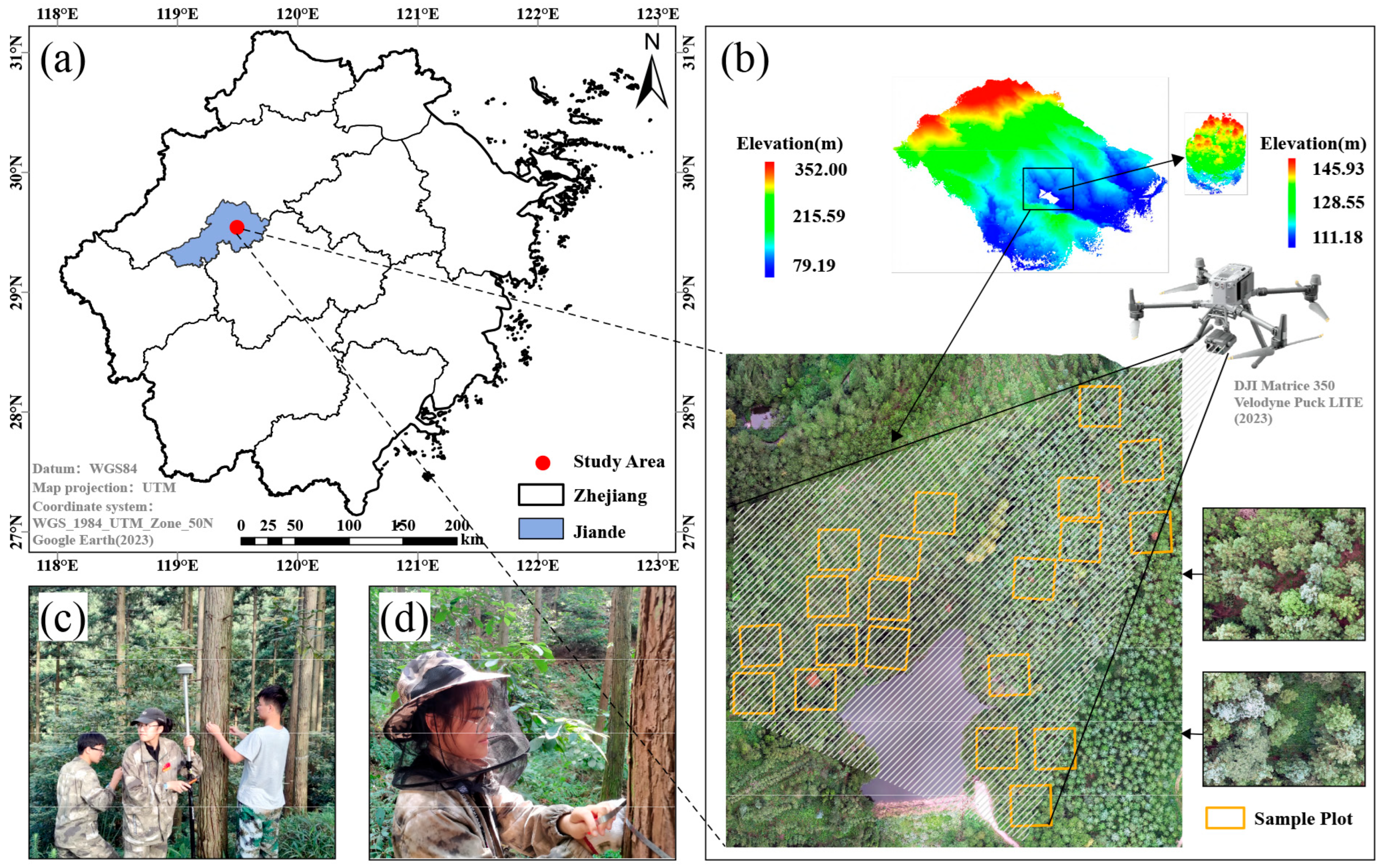
Figure 1. Overview of the study area: (a) location of Kinder (Datum: WGS84; Map projection: UTM; coordinate system: WGS_1984_UTM_Zone_50N; data source: Google Earth (2023)); (b) UAV point cloud data of the study area (collected using a DJI Matrice 350 equipped with a Velodyne Puck LITE LiDAR scanner) and RGB imagery; (c) RTK mono-log positioning; and (d) field measurements.
Remotesensing 17 02842 g001
Figure 2. The flowchart for this study.
Remotesensing 17 02842 g002
Figure 3. Example of calculation of space structure parameters.
Remotesensing 17 02842 g003
Figure 4. Individual Chinese fir tree segmentation results based on seed points (a) and local comparisons with point cloud segmentation results (b,c).
Remotesensing 17 02842 g004
Figure 5. Univariate distributions of structural parameters of Chinese fir. (a) The univariate distribution of parameters C, U, and W. (b) The univariate distribution of parameters CI. (c) The univariate distribution of parameters K.
Remotesensing 17 02842 g005
Figure 6. Bivariate distributions of stand spatial structural parameters (a) combination of W and U (Dark blue indicates U = 0, light blue indicates U = 0.25, light pink indicates U = 0.5, pink indicates U = 0.75, and dark pink indicates U = 1); (b) combination of W and C (Dark blue indicates C = 0, light blue indicates C = 0.25, light pink indicates C = 0.5, pink indicates C = 0.75, and dark pink indicates C = 1); (c) combination of U and C (Dark blue indicates C = 0, light blue indicates C = 0.25, light pink indicates C = 0.5, pink indicates C = 0.75, and dark pink indicates C = 1).
Remotesensing 17 02842 g006
Figure 7. Trivariate distribution of stand spatial structural parameters.
Remotesensing 17 02842 g007
Figure 8. Correlations between spatial structural parameters and AGB in Chinese fir stands. In the figure, the darker the red color, the more frequently the dots appear; the darker the blue color, the more scattered or less frequent the dots appear.
Remotesensing 17 02842 g008
Figure 9. Importance analysis of spatial structure parameters. (f) The degree of influence of parameters U, CI, K and C on AGB.
Remotesensing 17 02842 g009
Figure 10. Analysis of the importance of feature variables based on the RF (a) and XGBoost (b) models.
Remotesensing 17 02842 g010
Figure 11. Accuracy results of estimating AGB based on the XGBoost, CatBoost, KNN, and RF models in Scheme 1 and Scheme 2, and 3. (a) Scheme 1 estimates the AGB results based on the XGBoost model. (b) Scheme 2 estimates the AGB results based on the XGBoost model. (c) Scheme 3 estimates the AGB results based on the XGBoost model. (d) Scheme 1 estimates the AGB results based on the CatBoost model. (e) Scheme 2 estimates the AGB results based on the CatBoost model. (f) Scheme 3 estimates the AGB results based on the CatBoost model. (g) Scheme 1 estimates the AGB results based on the KNN model. (h) Scheme 2 estimates the AGB results based on the KNN model. (i) Scheme 3 estimates the AGB results based on the KNN model. (j) Scheme 1 estimates the AGB results based on the RF model. (k) Scheme 2 estimates the AGB results based on the RF model. (l) Scheme 3 estimates the AGB results based on the RF model. In the figure, the darker the red color, the more frequently the dots appear; the darker the blue color, the more scattered or less frequent the dots appear.
Remotesensing 17 02842 g011
Figure 12. Spatial distribution of structural parameters U, C, CI, and K. (a) The spatial distribution of structural parameter U. (b) The spatial distribution of structural parameter C. (c) The spatial distribution of structural parameter CI. (d) The spatial distribution of structural parameter K.
Remotesensing 17 02842 g012
Figure 13. Spatial distribution, scatter plot, and frequency distribution of AGB estimated based on Scheme 1 ((a) spatial distribution of AGB; (b) AGB estimation scatter plot; (c) actual AGB frequency distribution; (d) predicted AGB frequency distribution).
Remotesensing 17 02842 g013
Figure 14. Spatial distribution, scatter plot, and frequency distribution of AGB estimated based on Scheme 2 ((a) spatial distribution of AGB; (b) AGB estimation scatter plot; (c) actual AGB frequency distribution; (d) predicted AGB frequency distribution).
Remotesensing 17 02842 g014
Figure 15. Spatial distribution, scatter plot, and frequency distribution of AGB estimated based on Scheme 3 ((a) spatial distribution of AGB; (b) AGB estimation scatter plot; (c) actual AGB frequency distribution; (d) predicted AGB frequency distribution).
Remotesensing 17 02842 g015
Figure 16. q values of the parameters in Scheme 3 for AGB prediction.
Remotesensing 17 02842 g016
Table 1. Parameters of the LIDAR system.
ParametersUAV-LiDAR
transducersH300-RT (1 pc)
maximum pitch angle30°
laser wavelength905 nm
altitude (aviation)60 m
flight speed8 m/s
maximum horizontal flight speed23 m/s
ranging accuracy±1 cm (0.5 cm)
scanning frequency20 Hz
scanning frequency300 kHz
wavelength905 nm
Table 2. Field survey information.
Statistical CharacteristicMin (cm)Max (cm)Average Value (cm)Extremely Poor (cm)Standard Deviation (cm)
DBH0.393.916.393.69.9
Table 3. Equations for space structure parameters.
Spatial Structure ParametersFormulasAccount forPartition
Neighborhood comparison U = 1 n j = 1 n K i j Kij = 1 when competing wood j is smaller in diameter at breast height than object wood i; otherwise Kij = 0 Five classes of 0, 0.25, 0.5, 0.75, and 1 [48]
Crowding degree C = 1 n j = 1 n Y i j Yij = 1 when object wood i overlaps the crown projection of neighboring wood j; otherwise Y(ij) = 0 Five classes of 0, 0.25, 0.5, 0.75, and 1 [48]
Uniform angular scale W = 1 n j = 1 n Z i j When the jth angle α is smaller than the standard angle α0, Zij = 1; otherwise Zij = 0 Five classes of 0, 0.25, 0.5, 0.75, and 1 [48]
Hegyi competition index C I = j = 1 n d j d i × L i j Lij is the distance between the object tree and the competing tree (m), di is the diameter at breast height (cm) of the object tree, dj is the diameter at breast height (cm) of the competing tree, and n is the number of competing trees (plants) of the object tree (0, 0.2], (0.2, 0.8], (0.8, 1.4], (1.4, 2.0], and (2.0, ∞] [23]
openness K = 1 n j = 1 n L i j H i j Lij is the horizontal distance (m) between the object wood and the nearest neighbor wood j, Hij is the tree height (m) of the nearest neighbor wood at distance i, and n is the number of competing trees (plants) of the object wood (0, 0.2], (0.2, 0.3],
(0.3, 0.4], (0.4, 0.5],
(0.5, ∞] [49]
Table 4. Description of LiDAR-derived feature variables.
ULS Feature VariableVariable DescriptionReference
Height-Based Metrics [54]Height Percentiles (H5, H10, H20, H25, H30, H40, H50, H60, H70, H75, H80, H90, H95, H99)Percentiles of first-return height values (5th, 10th, 20th, 25th, 30th, 40th, 50th, 60th, 70th, 75th, 80th, 90th, 95th, and 99th)[54,55,56]
Coefficient of Variation (Hcv)Coefficient of variation of the first-return point cloud heights
Maximum Height (Hmax)Maximum tree height from first-return point cloud
Variance (Hva)Variance of first-return point cloud heights
Standard Deviation (Hstd)Standard deviation of first-return point cloud heights
Median Height (Hmed)Median of first-return point cloud heights
Mean Height (Hmean)Mean value of first-return point cloud heights
Interquartile RangeInterquartile range of first-return point cloud heights
Root Mean Square Height (Hsq)Root mean square of first-return point cloud heights
Cubic Mean Height (Hcm)Cubic mean of first-return point cloud heights
Density-Based Metrics (DB)Canopy Return Densities (D0, D1, D2, D3, D4, D5, D6, D7, D8, D9)Percentage of points above certain height percentiles (10th to 90th) relative to total number of points[57]
Canopy Structure Metrics (CS)Crown Area (S)Projected crown area calculated using a 2D convex hull algorithm[58]
Crown Diameter (CD)Average diameter of the crown point cloud: ( X m a x     X m i n )   +   ( Y m a x     Y m i n ) 2
Crown Volume (V)Crown volume calculated using a 3D convex hull algorithm
Table 5. Accuracy evaluation of individual tree segmentation.
NtNoNcrpF
Point Cloud Segmentation4301239178%82%80%
Seed Point-Based Segmentation521645989%90%89%
Disclaimer/Publisher’s Note: The statements, opinions and data contained in all publications are solely those of the individual author(s) and contributor(s) and not of MDPI and/or the editor(s). MDPI and/or the editor(s) disclaim responsibility for any injury to people or property resulting from any ideas, methods, instructions or products referred to in the content.