Quantifying Emissivity Uncertainty in Multi-Angle Long-Wave Infrared Hyperspectral Data

Abstract

This study quantifies emissivity uncertainty using a new, specifically collected multi-angle thermal hyperspectral dataset, Nittany Radiance. Unlike previous research that primarily relied on model-based simulations, multispectral satellite imagery, or laboratory measurements, we use airborne hyperspectral long-wave infrared (LWIR) data captured from multiple viewing angles. The data was collected using the Blue Heron LWIR hyperspectral imaging sensor, flown on a light aircraft in a circular orbit centered on the Penn State University campus. This sensor, with 256 spectral bands (7.56–13.52 μm), captures multiple overlapping images with varying ranges and angles. We analyzed nine different natural and man-made targets across varying viewing geometries. We present a multi-angle atmospheric correction method, similar to FLAASH-IR, modified for multi-angle scenarios. Our results show that emissivity remains relatively stable at viewing zenith angles between 40 and 50° but decreases as angles exceed 50°. We found that emissivity uncertainty varies across the spectral range, with the 10.14–11.05 μm region showing the greatest stability (standard deviations typically below 0.005), while uncertainty increases significantly in regions with strong atmospheric absorption features, particularly around 12.6 μm. These results show how reliable multi-angle hyperspectral measurements are and why angle-specific atmospheric correction matters for non-nadir imaging applications

1. Introduction

Hyperspectral remote sensing methods, which enable the collection of information about objects without physical contact, have become increasingly prevalent across many scientific and industrial applications. Long-wave infrared (LWIR) remote sensing techniques have gained significant traction due to recent advances in sensor technology that provide enhanced spectral and spatial resolution. These methods leverage measurements of radiation emitted across dozens or even hundreds of bands of the electromagnetic spectrum, enabling precise identification of materials and chemical compounds [1,2]. This capability is useful across diverse applications, including mineral exploration [3,4], detection of gas leaks and volatile organic compounds [5,6], environmental pollution analysis [7], soil property characterization [8], and building envelope assessment [9], with specialized instruments being developed for natural resources applications [10]. Recent reviews have highlighted the expanding role of UAV-based hyperspectral sensors in agricultural and forestry applications [11], while thermal infrared remote sensing continues to advance in precision agriculture [12] and crop water-stress detection [13].

While fundamental methods for remote sensing material identification were established decades ago [1], these traditional approaches rely on multiple simplifying assumptions that often lead to suboptimal performance under real-world data collection conditions. Several factors contribute to uncertainty and non-reproducibility, including material mixtures, shadows, instrumental noise, and particularly atmospheric effects that distort the measured signal. One promising approach to potentially improve material identification under these challenging conditions involves capturing and jointly processing images of the same scenes from multiple viewing angles in rapid succession [14,15].

An important limitation in the current remote sensing approaches is the assumption that targets of interest behave as Lambertian reflectors/emitters, meaning they emit radiation consistently regardless of the observer’s angle. While it is theoretically possible to characterize the relationship between emitted-reflected radiation and observer angle through the Bidirectional Reflectance Distribution Function (BRDF), such measurements are challenging [16]. They typically require controlled laboratory conditions and cannot be readily obtained for the diverse range of materials and material mixtures encountered in real-world remote sensing scenarios.

The literature suggests that angular variation in emissivity (defined as the ratio between the radiance emitted by the object and the radiance emitted by a black body at the same temperature) is caused by two processes: the intrinsic anisotropic emissivity of Earth materials and the thermal heterogeneity of complex, 3D land targets. Numerous studies have aimed to measure the directional emissivity of soil, leaves, and other natural surfaces, noting that the emissivity of such surfaces generally decreases with an increasing view zenith angle in the LWIR (8–14 μm) band [17,18]. A review by Cao et al. [19] synthesizes decades of research on Earth surface thermal radiation directionality, showing the complexity of angular effects across different surface types. Different types of land surface materials exhibit different angular variations in emissivity, with arid bare soils and water showing the highest angular dependence. The Fresnel reflectance theory effectively predicts the angular variations in emissivity for smooth surfaces like bare ice [20]. However, the observed angular behavior at a local scale may not always match that at a larger scale. Factors such as the structure of the surface, the proportion of reflective soil, and the combined impact of surface slope and sensor’s scan angle can result in large angular dependence of emissivity, even exceeding 60° in certain circumstances [21]. For example, Ermida et al. [22] compare the emissivities of desert region materials using satellite imagery from multiple satellites. However, the satellite-based method faces significant limitations since individual satellites maintain constant imaging angles, necessitating the use of multiple satellites to achieve angle diversity. This approach still provides relatively limited angular coverage and can only effectively analyze large homogeneous areas such as deserts and oceans, severely restricting the diversity of surface materials that can be studied. Validation efforts for satellite-derived land surface temperature products have further demonstrated the challenges of accounting for angular emissivity effects in operational products [23].

But before the emissivity can be derived from the remote sensing imagery, one needs to account for the influence of the atmosphere on the measured signal. This is commonly referred to as atmospheric correction. Hyperspectral remote sensing images in the LWIR region contain multiple signal components. These include atmospheric upwelling (path) radiance that adds to the measured signal, atmospheric downwelling or self-emission radiance that reflects from surfaces, and atmospheric transmittance, which attenuates the measured signal. To extract meaningful target information, these atmospheric constituents must be accurately accounted for. Since our primary interest lies in object emissivity, we must perform temperature-emissivity separation (TES). This represents an ill-posed problem since target temperatures are not known a priori. While numerous methods have been developed to address both atmospheric correction and TES, most existing approaches are not optimized for non-nadir imaging at varying angles. Xu et al. [14] focused on developing atmospheric correction methods specifically for multi-angle imagery. Their work introduced machine learning-based approaches to emulate atmospheric energy transfer, simulated using the MODTRAN (MODerate resolution atmospheric TRANsmission) radiative transfer code. Unlike conventional solutions that consider imaging and atmospheric correction in the nadir position, this work investigated atmospheric correction of the imagery captured from multiple angles and ranges. However, a notable limitation of this study is that it relied on MODTRAN simulations rather than data collected under real-world conditions.

Atmospheric influence can be addressed through either physics-based modeling of atmospheric energy transfer or direct extraction of TUD (transmission/upwelling/downwelling) atmospheric profiles from the scene itself. Multiple atmospheric models were developed, and they yield very close results as they attempt to characterize the same physical phenomena [14]. Perhaps the most challenging step of using atmospheric radiation propagation models is that these models require initialization with scene-specific atmospheric conditions, including imaging date/time, atmospheric pressure, humidity, and temperature profiles. Such parameters are rarely known prior to imaging. These atmospheric profiles can be obtained either from aerosonde soundings (which are rarely available during measurement) or through grid search methods that identify parameters best fitting the measurement conditions. The issue with this method is that multiple physically incorrect atmospheric parameters can lead to a plausible but incorrect atmospheric profile. Also, physics-based modeling approaches are computationally intensive and slow. To address this limitation, regression-based and machine learning methods have been developed to emulate model outputs, significantly reducing computational requirements [24].

Given the challenges in precise atmospheric characterization during imaging, in-scene atmospheric correction methods capable of extracting the TUD profiles from the scene itself without relying on the physics-based models have been developed. For LWIR hyperspectral imaging, two prominent approaches are ISAC [25] and QUAC-IR [26]. ISAC (in-scene atmospheric correction) operates on the assumption that black-body-like targets are present within the input scene, which is true for most natural scenes. It identifies these materials and derives atmospheric transmission and upwelling parameters by analyzing the relationship between brightness temperature and radiance across spectral bands. The resulting parameters are “unscaled,” approximating the shape of transmission and upwelling profiles without proper physical units, requiring subsequent scaling using MODTRAN estimates or water vapor band data. Recent advances in machine learning have shown promise for atmospheric correction, with deep neural networks demonstrating improved performance for time-dependent atmospheric parameter retrieval [27]. A limitation of ISAC is its inability to provide downwelling spectra information necessary for characterizing reflective targets. QUAC-IR (Quick Atmospheric Correction—Infrared) employs a more sophisticated approach, beginning with a random (Monte-Carlo) pixel selection to identify potential black-body materials through comparison with theoretical black-body radiance at specific wavelengths. It then uses regression techniques to determine upwelling and transmittance quantities and applies empirical relationships to calculate downwelling radiance spectra. Thompson et al. [28] provide a comprehensive review of atmospheric parameter retrieval methods for imaging spectroscopy.

A significant limitation of existing methods is their optimal performance only in nadir-position imaging. Adapting these approaches for slant-range viewpoints requires modifications to account for angle and range-dependent signal variations. Research on atmospheric correction for non-nadir multi-angle imagery in the LWIR domain remains limited. Only two in-scene atmospheric correction implementations have addressed slant-range correction: one approach involved manual segmentation of slant-range images followed by ISAC application to image segments [29], while O’Keefe later developed a modified ISAC method incorporating range-dependent variations in downwelling/upwelling/transmittance derived from MODTRAN simulations [30]. The latter approach demonstrated superior performance compared to segmentation methods, providing more realistic material emissivity distributions without artificial discontinuities at segment boundaries. However, fundamental performance limitations in temperature-emissivity separation remain a significant challenge for LWIR hyperspectral applications, particularly in complex scenes [31].

As one can see, the methods necessary for characterizing emissivity uncertainty in multi-angle rapid imagery collection are available, with the critical missing component being real-world LWIR imaging data showing various targets at different angles. Our work addresses this gap through the Nittany Radiance LWIR imaging dataset [32]. This dataset will be detailed in the subsequent data section.

This paper makes two primary contributions to the field:

• The adaptation of existing atmospheric compensation algorithms for multi-angle scenarios, addressing their traditional performance degradation in non-nadir conditions.
• An evaluation of emissivity uncertainty distribution across different targets in the imaging area, providing insights into the reliability of multi-angle hyperspectral measurements.

2. Data

Nittany Radiance was an airborne data collection mission that used the Blue Heron hyperspectral sensor over the campus of Pennsylvania State University to collect multiple hyperspectral images.

Blue Heron is a hyperspectral camera that works in a thermal infrared wavelength range (7.56–13.52 μm) with 256 spectral bands and a spectral sampling of approximately 0.023 μm (23 nm) per channel. The sensor has an across-track field of view (FOV) of approximately 1.79° and an along-track FOV of 2.12°, with corresponding instantaneous field of view (IFOV) values of 0.121 mrad (across-track) and 0.100 mrad (along-track). The camera is mounted on a gimbal and is capable of imaging the scene from different angles in a fast sequence. The camera has two push-broom side-looking imaging sensors, called side 1 and side 2, which allow for capturing a wider swath of the scene of interest with a typical swath width of approximately 146 m. Scene is scanned line-by-line, and each line (row) in the image has a different camera-to-scene range and gimbal elevation angles. The sensor was mounted on a Cessna Grand Caravan aircraft. It collected data in a circular orbit, steering the gimballed sensor at a fixed location, to derive the spectral data at multiple angles for the Lambertian surface targets as well as volatile organic compounds released at two sites on campus.

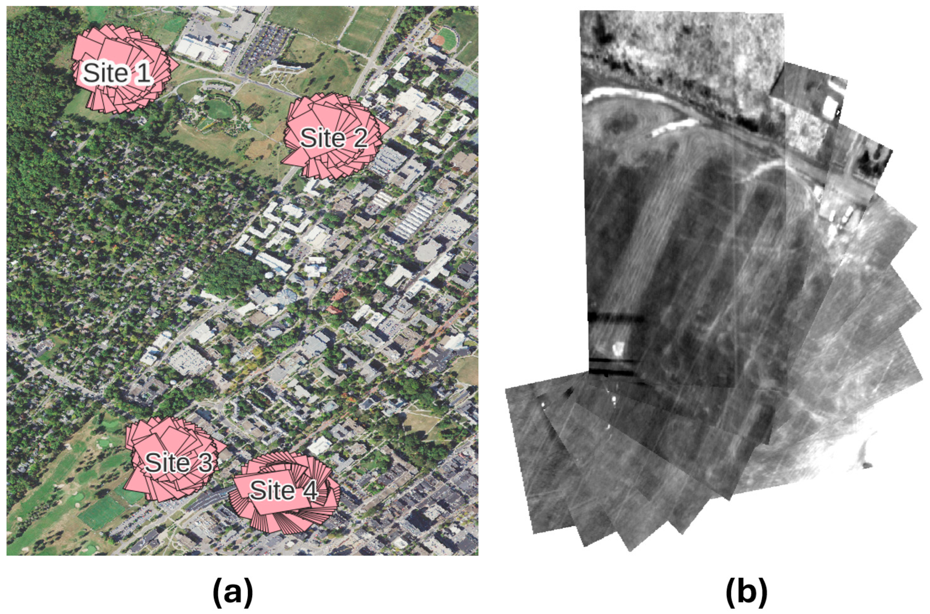
The acquired images have dimensions of 258 pixels across-track and 370 pixels along-track, covering ground areas of approximately 146 × 172 m. Spatial sampling varies with flight altitude and viewing geometry, with typical across-track and along-track resolutions of 0.57 m and 0.47 m, respectively. The aircraft was flown at altitudes of approximately 3400 m above ground level, with slant ranges to targets varying between approximately 4100–5700 m, depending on viewing angle and target location. The camera images multiple sites simultaneously in one camera run. The resulting images are organized within folders, one folder for each camera run. We refer to the images from a single folder as a “group” or “batch”. Each batch contains approximately 14 images. The camera is recalibrated using a black body radiation source before each run. Each folder has images covering multiple sites. There are five distinct sites covering the PSU campus. In the experiments, about 5 to 14 images in the batch spatially overlapped with the selected spectral target of interest. 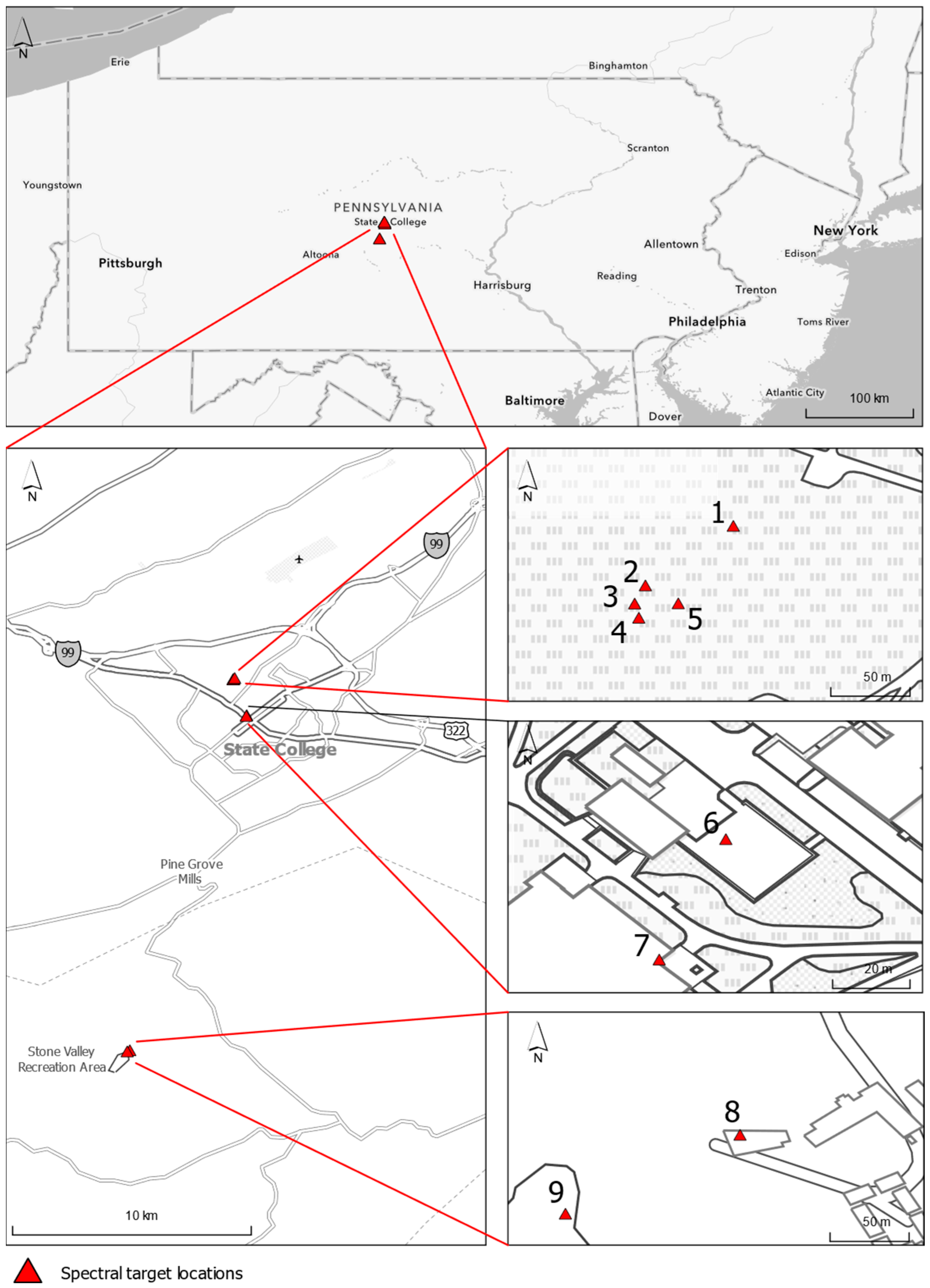Close-up locations of the most imaging sites are shown in Figure 1, and the reference map, explaining the geographic location of the imaging sites and corresponding targets, is provided in Figure 2.

Data preparation: Pixels from different images at approximately the same geographic location were selected. There are two problems: the georeferencing of the images is challenging due to the small overlap between the images and the limited number of usable control points. This is possible to overcome by selecting points of interest manually at each image. The extraction window—a rectangular area geographically centered at the spectral target of interest—was used to obtain representative spectra from each location. When using larger extraction windows (containing multiple pixels whose spectra are averaged), there is a good chance that pixels belonging to materials of different types will be included. Conversely, when using a single-pixel extraction window, the results are more susceptible to noise, or the selected pixel could represent mixed materials. For this study, a 3 × 3-pixel extraction window was used, and the extracted spectra from these pixels were averaged.

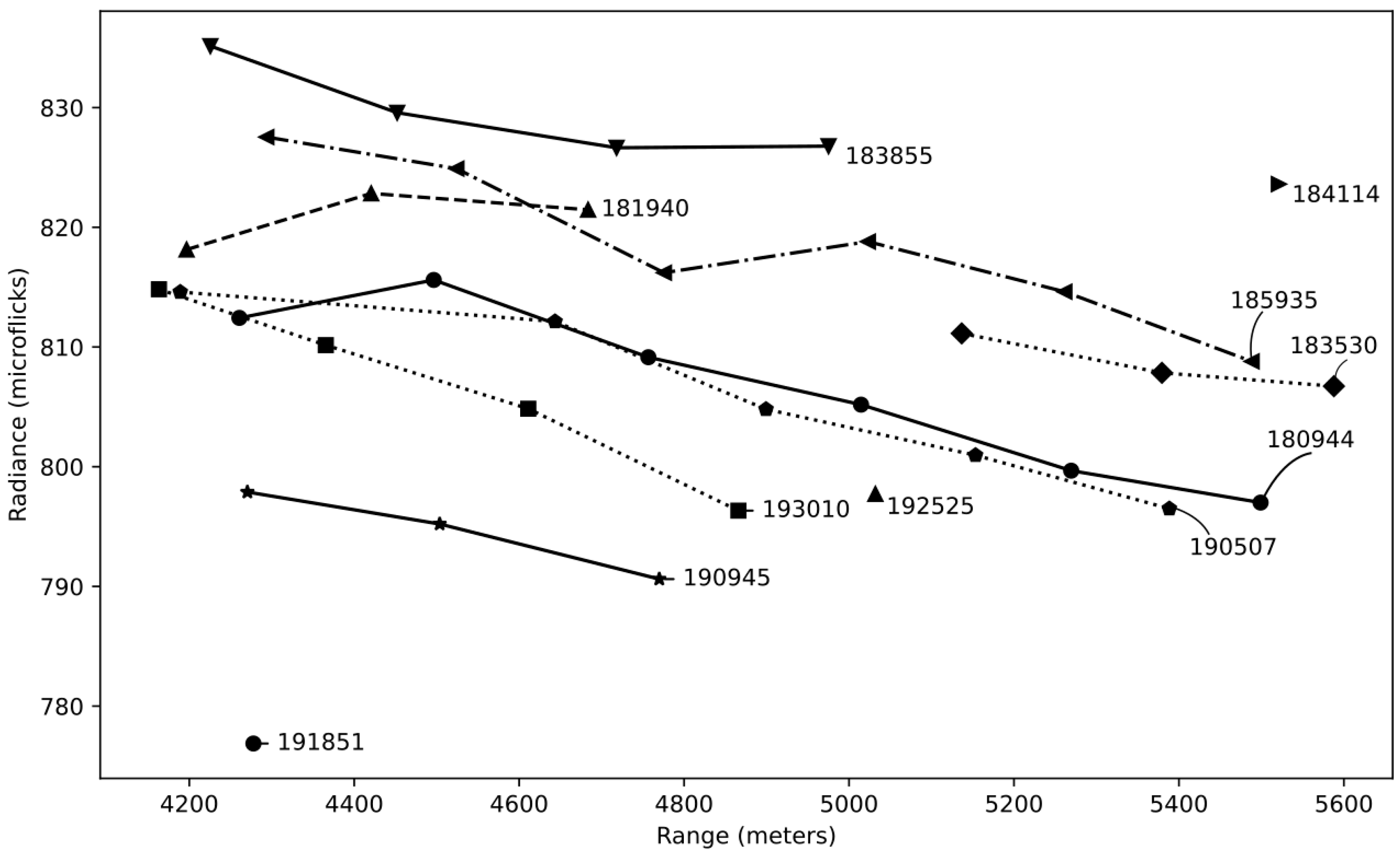
The other problem is that there is an abrupt change in radiance between different batches of the images. The imager is capturing the scenes in one rapid sequence of about 8–16 images. Then the sensor re-calibrates using the built-in black-body radiation source and captures the next image sequence. Radiance generally smoothly decreases with the path length increase, but this is true only if the images belong to a single batch (folder). They are not directly inter-comparable between the different folders. To overcome this, one can only look at the images within a single batch, which leads to a smaller range of observed angles compared to the use of all available images. For the “buildings” site, the difference in calibration is relatively small, and it was possible to use images from three separate batches. This problem is exemplified in Figure 3.

Each line (row) in the image is associated with its own imaging angle and range, which were recorded during the data collection. These ranges and angles were retrieved from the image metadata (telemetry and input geometry files) supplied with the source images.

Keeping this in mind, the following nine different targets listed in

Table 1. Targets selected for further analysis.

Target Name	Number of Images	Angular Range (°)	Path Length Range (m)
Site 1—Arboretum
Arboretum grass	5	49.76–57.02	4810–5717
Arboretum grass 1	7	41.27–55.68	4140–5531
Arboretum panel	6	40.97–55.68	4122–5315
Arboretum pond	6	40.97–55.68	4334–5534
Arboretum tarp	5	47.48–55.76	4600–5547
Site 4—Buildings
Walker building roof	14	44.51–51.78	4345–5010
Columbia Gas gravel site	14	44.40–51.45	4345–5010
Site 5—Shavers Creek
Shavers Creek wetland	10	48.56–49.07	4841–4885
Shavers Creek roof	10	47.88–48.47	4756–4808

were selected:

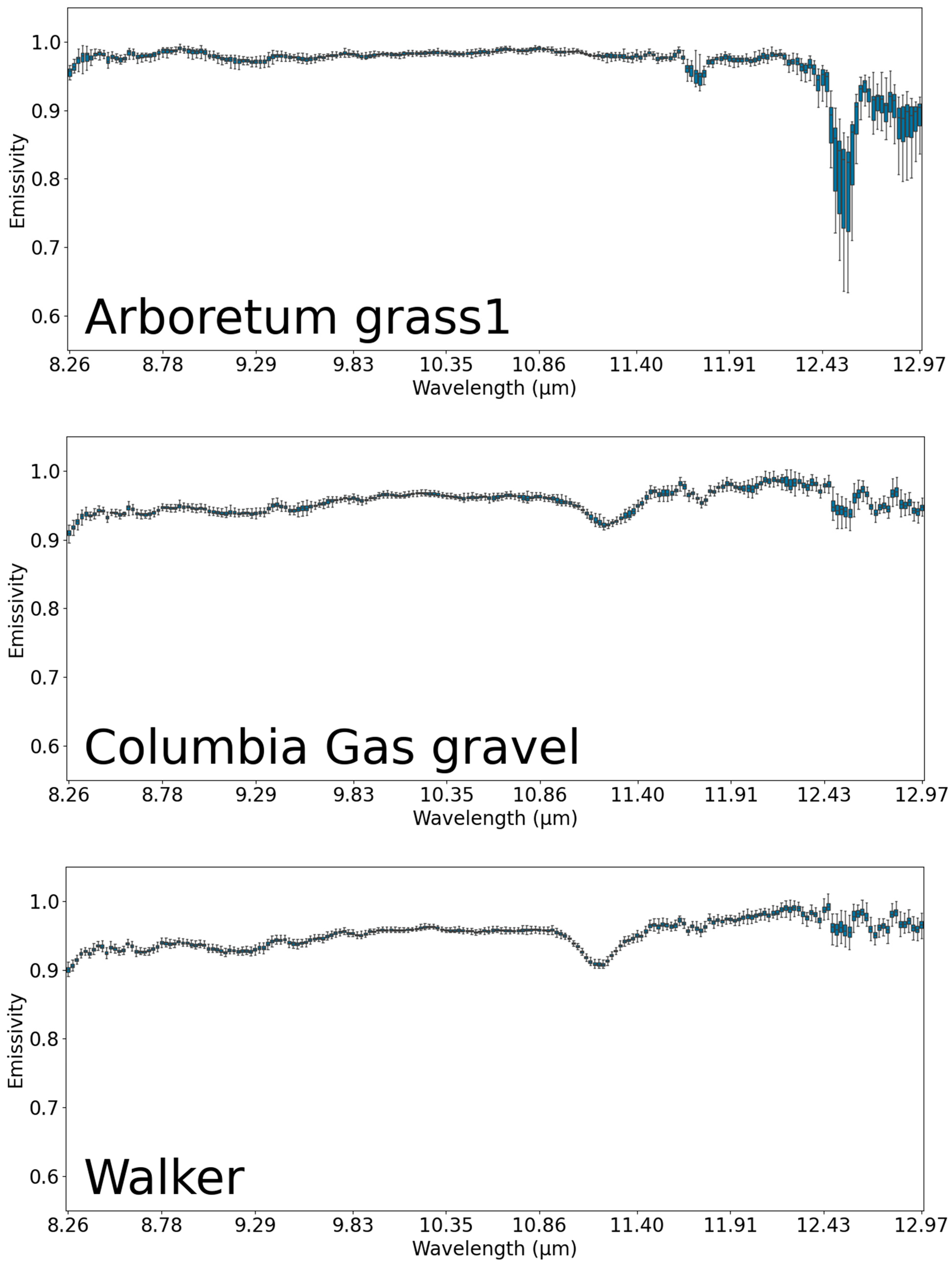
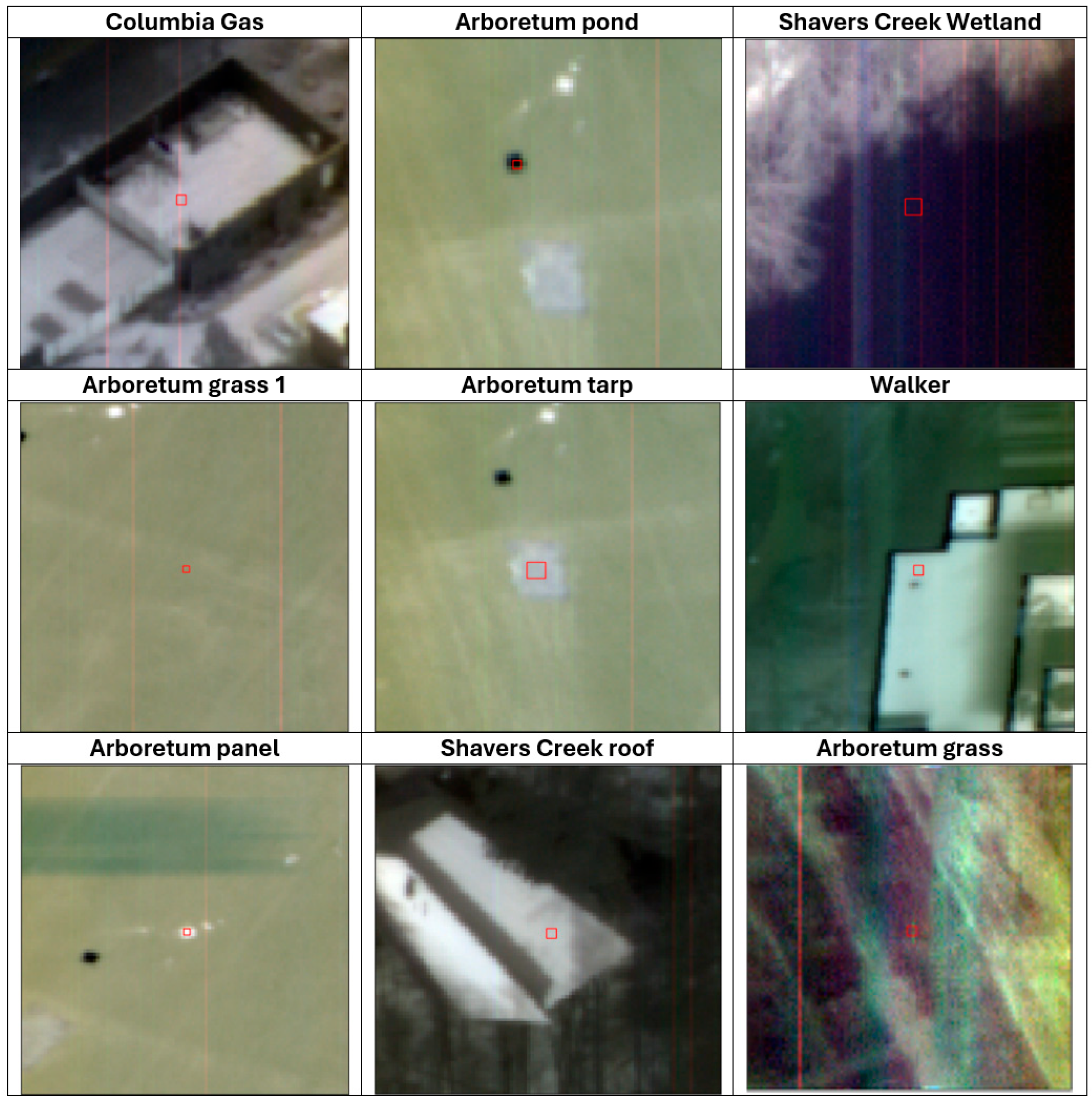
A more detailed overview of the target appearances is provided in Figure 4.

3. Methods

This section explains our data processing workflow for extracting material emissivity spectra from Nittany Radiance LWIR hyperspectral multi-angle imagery. We began by calculating ground coordinates, ranges, and angles from telemetry metadata for each pixel of interest.

After resolving geometric parameters, we performed atmospheric correction by adapting an approach similar to the FLAASH-IR atmospheric correction method to the multi-angle scenario. We started by modeling multiple trial atmospheres in the MODTRAN 6.0.1 radiative transfer model, systematically varying water vapor, ozone, and temperature parameters until finding optimal transmission, upwelling, and downwelling (TUD) profiles that matched reference water spectra. While the original FLAASH-IR method uses a smooth spectra assumption for both matching candidate atmospheres and temperature-emissivity separation, we instead relied on matching with reference water spectra to find the optimal atmosphere. Using these atmosphere-specific parameters, we implemented a temperature-emissivity separation algorithm that maximizes spectral smoothness to derive material emissivity spectra. Finally, we analyzed the derived emissivity spectra to look at angular emissivity dependence and distribution. 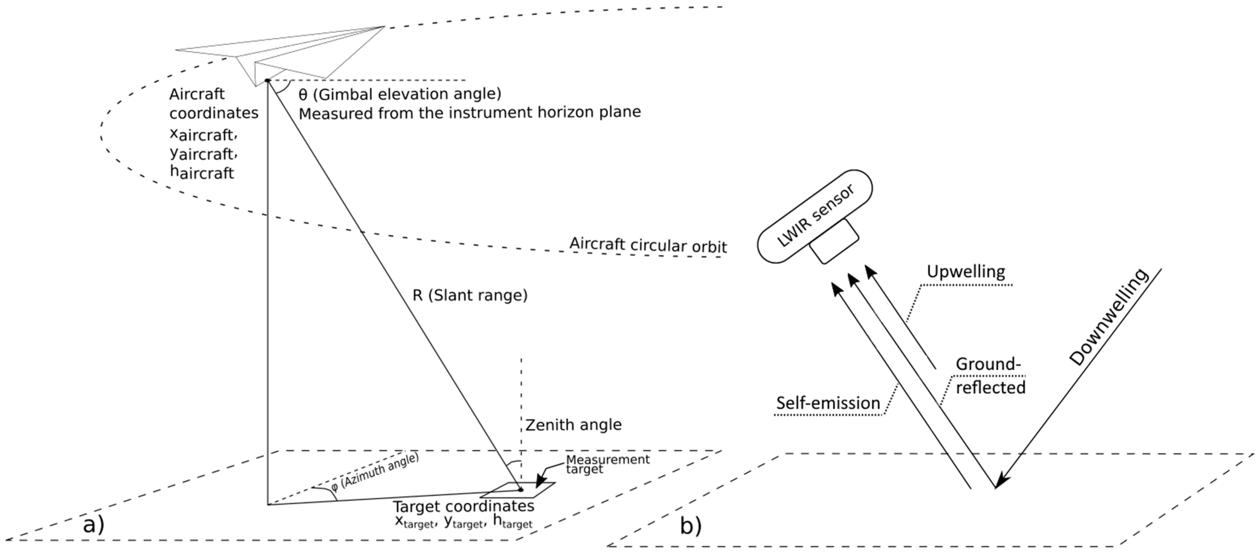The data processing workflow is presented in Figure 5, and the data collection geometric setting is presented in Figure 6. We describe these processes in more detail below.

3.1. Geometry Resolution

The data processing workflow started with resolving the image acquisition geometry, that is, by determining ground coordinates of the pixels and range calculation, which were further used in the atmospheric correction process. To determine the ground coordinates of pixels captured by the airborne imaging system, we employed a geometric projection method based on the aircraft’s position, sensor orientation, and terrain elevation. This is referred to as “resolve” geometry process in Figure 5.

The geometric relationship between aircraft, sensor, and ground targets is illustrated in Figure 6a. The process of calculating pixel ground coordinates from the telemetry data follows these steps:

• We corrected the sensor angles by applying calibration offsets:

  $${\theta }_{\mathit{corrected}}={\theta }_{\mathit{measured}}-\Delta \theta$$

  (1)

  $${\varphi }_{\mathit{corrected}}={\varphi }_{\mathit{measured}}+\Delta \varphi$$

  (2)

  where $\theta$ is the gimbal elevation angle (measured from the horizon plane), ϕ is the heading angle (azimuth), and $\Delta \theta$ = 0.2958° and $\Delta \varphi$ = 1.8654° are the respective calibration adjustments.
• The slant range distance (R) from aircraft to ground point was calculated as

  $$R={\displaystyle \frac{h_{\mathit{aircraft}}-h_{\mathit{terrain}}}{\mathit{tan}\left(\left|{\theta }_{\mathit{corrected}}\right|\right)}}$$

  (3)
• Ground coordinates were then computed as

  $$x_{\mathit{ground}}=x_{\mathit{aircraft}}+R\times \mathit{sin}\left({\varphi }_{\mathit{corrected}}\right)$$

  (4)

  $$y_{\mathit{ground}}=y_{\mathit{aircraft}}+R\times \mathit{cos}\left({\varphi }_{\mathit{corrected}}\right)$$

  (5)

  where $x_{\mathit{aircraft}},y_{\mathit{aircraft}}$ represent the aircraft position, R is the calculated slant range, and ${\varphi }_{\mathit{corrected}}$ is the calibrated heading angle in radians.

3.2. Atmospheric Correction

To retrieve the emissive spectra of interest, one needs to account for the atmosphere contribution in the observed signal, which is dependent at the very least on atmospheric parameters, such as ozone and water vapor concentration, and atmospheric temperature. The observed at-sensor radiance in the infrared spectrum that is recorded for each pixel in the collected infrared images is modeled as

$$L_{obs}\left(\lambda \right)=B\left(T,\lambda \right)\epsilon \left(\lambda \right)\tau \left(\lambda \right)+\left[1-\epsilon \left(\lambda \right)\right]L^{\downarrow }\left(\lambda \right)+L^{\uparrow }\left(\lambda \right)$$

(6)

where $\lambda$ is wavelength, $B\left(T,\lambda \right)$ is a Planck black-body radiance function at the temperature T at wavelength $\lambda$, $\epsilon$ is the emissivity of the pixel, $\tau$ is an atmospheric transmittance between the sensor and target. $L^{\downarrow }$ is a downwelling radiance, $L^{\uparrow }$ is an upwelling radiance (or atmospheric self-emission) [14]. These atmospheric radiances are visually represented in Figure 6b. One can model the transmission $\tau$, $L^{\downarrow }$ and $L^{\uparrow }$ with the atmospheric radiation transport model, such as MODTRAN. To do so, one needs to know in advance or estimate the atmospheric parameters such as concentration of the atmospheric gases (water vapor and ozone) and atmospheric temperature.

For the 8–13 μm spectral region, water vapor is the most prominent atmospheric species [33], exhibiting thousands of absorption lines and continuum absorption [34]. Unlike well-mixed gases, water vapor varies substantially, with approximately 90% concentrated between the surface and 6 km altitude [34]. At the 3400 m sensor altitude, this variability below the sensor directly impacts atmospheric transmittance and path emission. Ozone contributes through upper atmospheric emission bands in the downwelling radiation [33]. Other gases (CO₂, CH₄) remain relatively stable as well-mixed constituents and can be represented using climatological values without significant modeling errors [34]. Therefore, water vapor and ozone require explicit parameterization in MODTRAN—water vapor for its dominant absorption/emission and high variability, and ozone for its downwelling contribution—while other gases can be treated as constants from standard atmospheric models. Since water vapor and ozone concentrations at the time of data collection are unknown, we generate multiple trial atmospheres with varying parameters and determine which combination best matches the measured radiance data.

3.3. Atmospheric Modeling

The atmospheric state was modeled using the MODTRAN 6.0.1 software. MODTRAN (MODerate resolution atmospheric TRANsmission) is a widely used radiative transfer model that simulates the propagation of electromagnetic radiation through the Earth’s atmosphere. The model calculates atmospheric transmission, upwelling (path radiance), and downwelling radiance across the electromagnetic spectrum by solving the radiative transfer equation using detailed atmospheric profiles of temperature, pressure, humidity, and trace gas concentrations. MODTRAN has become a standard tool in remote sensing applications for atmospheric correction and retrieval algorithms, as it provides the fundamental atmospheric parameters necessary for converting at-sensor radiance measurements to surface-leaving radiance [14,24].

Since the exact atmospheric parameters during the data collection were not known, one must create a look-up table by varying the water vapor concentration, ozone scale factor, and temperature of the lowest layer of the atmosphere. When modeling atmosphere states, one needs to specify the path geometry between the sensor and target. The geometry of the image where geometric parameters were selected closest to the median values of path range. The input geometry parameters are zenith angle of the observer, above mean sea level (AMSL) elevation of the observer, AMSL elevation of the ground target. With this set of geometry parameters, MODTRAN calculates the resulting path length automatically. The following parameter variations listed in

Table 2. MODTRAN atmospheric parameters for the trial atmospheres.

Parameter	Values	Step	Unit
H2O range	3000–4000	10	Atm. cm
O3 range	1.0–2.5	0.1	Scaled
Atm. T range	280–300	1	K

were used to generate trial atmospheres:

All possible combinations of these parameters with a single geometry were used to create the MODTRAN input files. A combination of these parameters with the specified steps allows us to create about 30,000 possible trial atmospheres, which takes about an hour to generate. The resulting MODTRAN “scanned” output contains the following columns of interest: wavelength, transmission, path emission, ground reflected radiance, and direct emissivity.

These modeled radiances can be separated into upwelling and downwelling radiance for further use in a radiometric equation as follows (combin_path_trans, path_emission, path_thermal_scat, grnd_reflect, direct_emiss are the original names of columns in the MODTRAN scanned output file):

$$\tau \left(\lambda \right)=combin\_path\_trans$$

(7)

$$L^{\uparrow }\left(\lambda \right)=L_{path\_emission}\left(\lambda \right)+L_{path\_thermal\_scat}\left(\lambda \right)$$

(8)

$$L^{\downarrow }\left(\lambda \right)={\displaystyle \frac{L_{grnd\_reflect}\left(\lambda \right)}{1-direct\_emiss}}$$

(9)

MODTRAN radiance units are W cm⁻² sr⁻¹/cm⁻¹ and to convert these to the microflicks (units of radiance used in the IR images), one needs to multiply MODTRAN values by a factor of 1 × 10⁶.

3.4. Search for the Appropriate Modeled Atmosphere

We selected the best trial atmosphere using the following approach: MODRAN-modeled TUD profiles, library water spectra, and varying ground target temperatures were used to reconstruct at-sensor water radiance. This reconstructed radiance was then compared with the radiance of the same material (water) extracted from the reference image. The atmospheric profile and target temperature that produced the lowest squared difference between reconstructed and observed spectra were selected as optimal.

To perform spectra comparison, we selected the area (15 × 15 pixels) of the water in the reference image. Also, an infrared water reflectivity spectrum was obtained from the ECOSTRESS spectral library. The reflectivity spectra were recalculated to emissivity, $\epsilon \left(\lambda \right)=1-r\left(\lambda \right)$, where $r\left(\lambda \right)$ is material reflectivity. The procedure works as follows:

For each MODTRAN atmospheric profile:

• We retrieve its TUD parameters (atmospheric transmission $\tau \left(\lambda \right)$, upwelling radiance $L^{\uparrow }\left(\lambda \right)$, and downwelling radiance $L^{\downarrow }\left(\lambda \right)$).
• For each trial temperature T (ranging from 280 to 320 K in 0.1 K steps), we plug these TUD parameters into the radiometric Equation (6) along with the following:

  -

  Water emissivity ${\epsilon }_{water}$ from the ECOSTRESS spectral library;

  -

  The Planck function $B\left(T,\lambda \right)$ at the current trial temperature.

• This gives us the reconstructed at-sensor radiance:

  $$L_{\epsilon }\left(\lambda \right)=B\left(T,\lambda \right)\cdot {\epsilon }_{water}\left(\lambda \right)\cdot \tau \left(\lambda \right)+\left[1-{\epsilon }_{water}\left(\lambda \right)\right]\cdot L^{\downarrow }\left(\lambda \right)+L^{\uparrow }\left(\lambda \right)$$

  (10)

  $L_{\epsilon }\left(\lambda \right)$ represents the reconstructed radiance spectra that the sensor would observe for water at temperature T under this specific atmospheric profile.
• We calculate the mean squared error (MSE) between this reconstructed radiance and the actual observed water radiance $L_{extracted}$ extracted from a 15 × 15-pixel water area in the reference image. We have calculated the error only for the narrower subset of the bands between the usable wavelengths range of 8.26–12.97 μm, which corresponds to the bands 30–232.

  $${\sigma }^2\left(T\right)={\displaystyle \frac{1}{N}}{\displaystyle \sum _{i=1}^N}{\left[L_{\mathit{extracted}}\left({\lambda }_i\right)-L_{\epsilon }\left({\lambda }_i,T\right)\right]}^2$$

  (11)

  where N is the number of spectral bands (30–232), $L_{\mathit{extracted}}$ is the observed radiance extracted from the reference image, $L_{\epsilon }\left({\lambda }_i,T\right)$ is the reconstructed radiance from Equation (10), ${\lambda }_i$ is the wavelength of the i-th band, and T is the trial temperature.
• We identify the optimal trial temperature T that minimizes ${\sigma }^2$ (MSE) for this atmospheric profile. After repeating this process for all MODTRAN profiles, we select the best TUD atmospheric profile and its corresponding optimal temperature that together produce the global minimum MSE. This combination represents the best estimate of the actual atmospheric conditions and water temperature during image acquisition.

It was not possible to find an ideal match (${\sigma }^2$ = 0) between the reconstructed and observed radiance spectra due to atmospheric modeling and calibration uncertainties, but there is a relatively close match as we define as ${\sigma }^2<{10}^{-5}\hspace{0.17em}{\left(\mathrm{W}\cdot {\mathrm{cm}}^{-2}\cdot {\mathrm{sr}}^{-1}\cdot \mathsf{\mu }{\mathrm{m}}^{-1}\right)}^2$ as can be seen in Figure 7 and Figure 8. Figure 7 shows the reconstructed radiance spectra according to Equation (10), and Figure 8 shows the comparison between the extracted and library emissive spectra of water.

The best TUD was selected with the following parameters: profile number: 16,980 out of 30,000, O₃: scale factor of 1.8, and H₂O of 3490 atm. cm. The selected TUD profile (highlighted in red in Figure 9) compares to all trial profiles in the following way:

3.5. Temperature—Emissivity Separation

To estimate the emissivity of materials in the images associated with different acquisition geometries, the atmospheric parameters must first be modeled for each specific geometry. This is accomplished by running MODTRAN multiple times, using the geometry parameters (zenith angle, aircraft, and target elevation) associated with each of the input images. The H₂O, O₃, and atmospheric temperature parameters retrieved in the previous step are used, assuming they remain unchanged during image collection in a rapid sequence. After generating the geometry-specific TUD profiles for the target geometry in each image, these parameters must be applied to the temperature-emissivity separation process.

Emissivity can be calculated by reformulating Equation (6) in the following way:

$$\epsilon \left(\lambda \right)={\displaystyle \frac{L_{extracted}\left(\lambda \right)-L^{\downarrow }\left(\lambda \right)-L^{\uparrow }\left(\lambda \right)}{B\left(T,\lambda \right)\cdot \tau \left(\lambda \right)-L^{\downarrow }\left(\lambda \right)}}$$

(12)

But the temperature of the target is unknown. Finding a feasible surface temperature and emissivity refers to a temperature-emissivity separation (TES) problem.

The “smooth emissivity” [35] assumption was employed to perform TES. Most natural materials exhibit a smooth emissivity spectrum, compared to sharp atmospheric features. By applying different trial temperatures, one can find the temperature that maximizes the smoothness of the resulting spectra.

The TES process works as follows:

For the trial temperature in the range 280–320 K with an increment of 0.1, the following is performed:

• Calculate the emissivity from the extracted radiance spectra using Equation (12).
• Smooth the calculated emissivity by calculating the running average across five spectral channels (uniform_filter1d is a NumPy function):

$${\epsilon }_{smoothed}=uniform\_filter1d\left(\epsilon \left(\lambda \right), size=5\right)$$

(13)

• Reconstruct the radiance spectra from the smoothed emissivity by inserting it into the radiometric Equation (6).

$$L_{{\epsilon }_{smoothed}}\left(\lambda \right)=B\left(T,\lambda \right){\epsilon }_{smoothed}\left(\lambda \right)\tau \left(\lambda \right)+\left[1-{\epsilon }_{smoothed}\left(\lambda \right)\right]L^{\downarrow }\left(\lambda \right)+L^{\uparrow }\left(\lambda \right)$$

(14)

• Calculate the mean squared difference between the extracted and reconstructed spectra.

$${\sigma }^2\left(T\right)={\displaystyle \frac{1}{N}}{\displaystyle \sum _{i=1}^N}{\left[L_{\mathit{extracted}}\left({\lambda }_i\right)-L_{{\epsilon }_{smoothed}}\left({\lambda }_i,T\right)\right]}^2$$

(15)

In Equation (15), $L_{{\epsilon }_{smoothed}}$ represents a radiance spectrum reconstructed from emissive spectra that have been smoothed using a running average across five bands, and $L_{extracted}$ is the original radiance spectrum extracted at the location of interest. The mean squared difference between $L_{extracted}$ and $L_{{\epsilon }_{smoothed}}$ decreases as the extracted spectra become smoother. Temperature values T were constrained between 280 and 320 K, and emissivity values between 0 and 1. Only bands 30–232 (corresponding to wavelengths 8.26–9.18 microns) were considered in the analysis. During each iteration cycle, the current ${\sigma }^2$ value is compared with the previous iteration to identify the minimum value, and the emissive spectrum corresponding to the lowest σ² is selected.

This process was repeated for each extracted spectrum of interest using the $\tau \left(\lambda \right)$, $L^{\downarrow }\left(\lambda \right)$ and $L^{\uparrow }\left(\lambda \right)$ from the corresponding MODTRAN simulation.

3.6. Emissivity Outlier Filtering and Recalculation

When extracting the pixels within some rectangular window, typically 3 × 3, it is possible to have the pixels belonging to different materials. They will be of different temperatures and different emissivities compared to the majority of pixels of interest. In this case, it is reasonable to filter these spectra out using the simple interquartile range filtering, removing the spectra outside of the ±1.5 interquartile range. The other way is to perform TES in two steps: retrieving emissivities and recalculating the emissivities using their median temperatures. In cases where the pixels indeed belong to different materials and the emissivities are different, this method does not provide good results.

Unlike the previous case, where outliers resulted from genuinely different materials within the sample pixels, an alternative scenario occurs when pixels represent the same material, but the smoothness maximization approach inadvertently selects the smoothest spectra from different images with significantly different temperatures. To address this issue, the median temperature is calculated for all pixels, and the outlier emissivity values are then recalculated using this median temperature value.

4. Results and Discussion

We estimated emissivities for nine spectral targets across three sites of interest, which include both natural and man-made surfaces. As shown in

Table 3. List of the imaging targets with their resolved temperature range and average emissivity. Y stands for the action was performed, N—not performed.

Target Name	Outlier Removal	Recalculate to Same T	Resolved T Range	Mean Emissivity
Site 1—Arboretum
Arboretum grass	Y	N	299.5–301.4	0.963
Arboretum grass 1	N	N	299.0–301.1	0.979
Arboretum panel	Y	N	301.0–315.0 1	0.974
Arboretum pond	N	N	281.0–292.0 2	0.566
Arboretum tarp	Y	Y	303.0–308.5 1	0.912
Site 4—Buildings
Walker building roof	N	N	313.2–314.6	0.985
Columbia Gas gravel	Y	N	309.0–310.5	0.955
Site 5—Shavers Creek
Shavers Creek wetland	Y	Y	291.0–293.5	0.963
Shavers Creek roof	Y	N	313.0–315.3	0.933

¹ indicates the spread of temperatures exceeding 3 degrees K, even after outlier removal and recalculation of the temperature (corrective actions) were performed. ² corrective actions did not improve the temperature range for this target.

, the emissivity values are relatively different between the different target types. Natural surfaces generally demonstrated high emissivity values, with Arboretum Grass (0.963), Shavers Creek Wetland (0.963), and Columbia Gas Gravel (0.955) all displaying values above 0.95. In contrast, man-made materials showed greater variability, with the Arboretum Pond exhibiting the lowest mean emissivity (0.566) among all targets.

Interestingly, some of the man-made targets did not follow this general pattern, such as the Walker Building roof (0.985) and black Arboretum Panel (0.974), displaying very high emissivity values comparable to natural surfaces, which can be attributed to their composition. These observations align with emissivity values reported in established spectral libraries, including the ECOSTRESS spectral library [36] and ASTER spectral library version 2.0 [37]. The Walker Building roof consists primarily of asphalt/stone materials, which typically exhibit high thermal emissivity properties like natural terrain. The outlier filtering procedure, applied to most targets, successfully removed anomalous measurements that could otherwise skew the results. Although we attempted recalculation to a standardized median temperature for all targets, this approach only produced a meaningful reduction in emissivity variation for two targets (Arboretum Tarp and Shavers Creek Wetland), suggesting that temperature standardization is not universally effective across different material types.

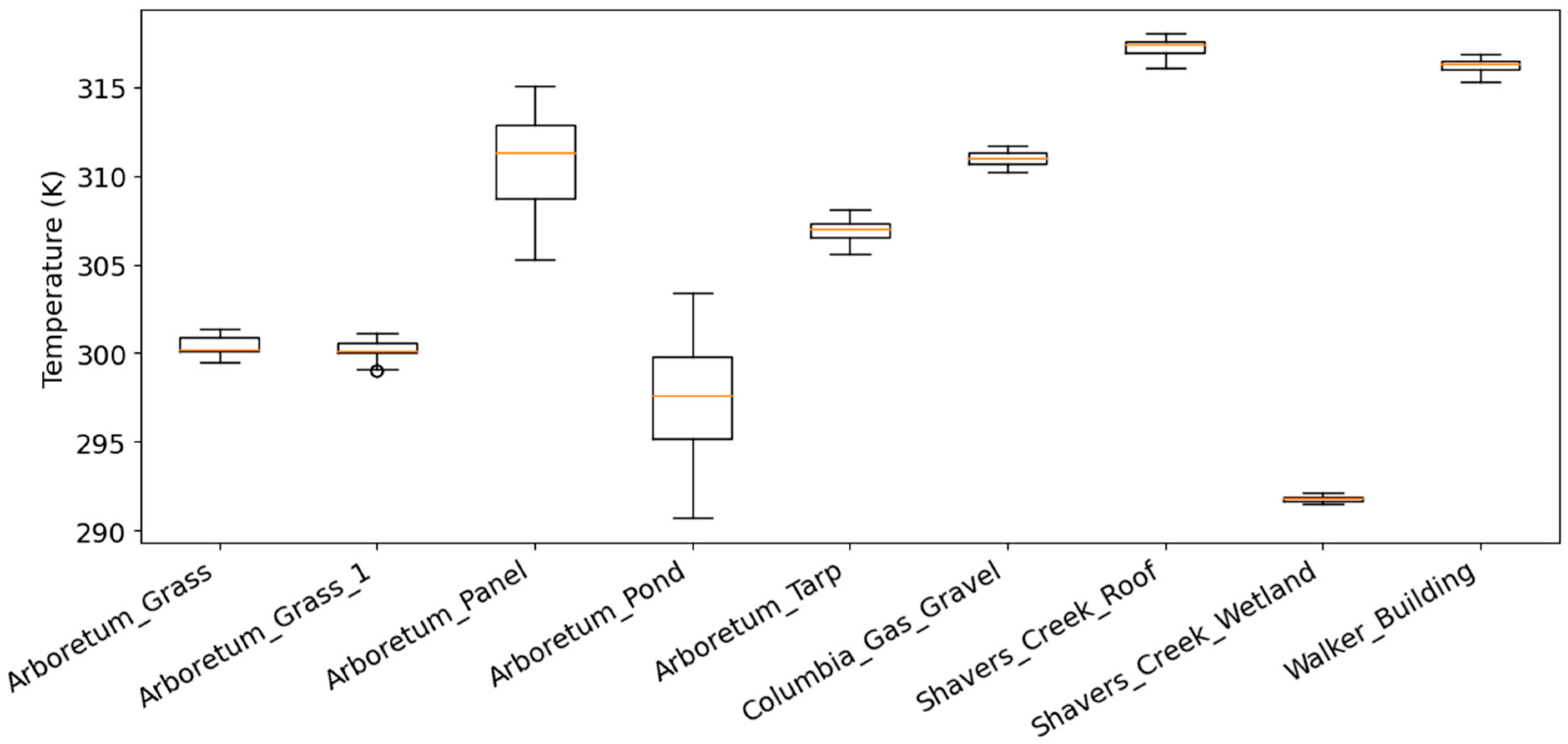
Temperature variability across targets (Figure 10) shows a great deal of thermal heterogeneity for some target types. While most targets exhibit relatively consistent temperatures, the Arboretum_Panel, Arboretum_Pond, and Arboretum_Tarp demonstrate much wider temperature ranges. The Arboretum panel exhibited the highest variation in temperatures (approximately 310–315 K), whereas the Arboretum_Pond target shows the lowest and most variable temperatures (approximately 290–305 K) due to the cooling effect of circulating water within the plastic structure.

4.1. Spectral Variation in Emissivity

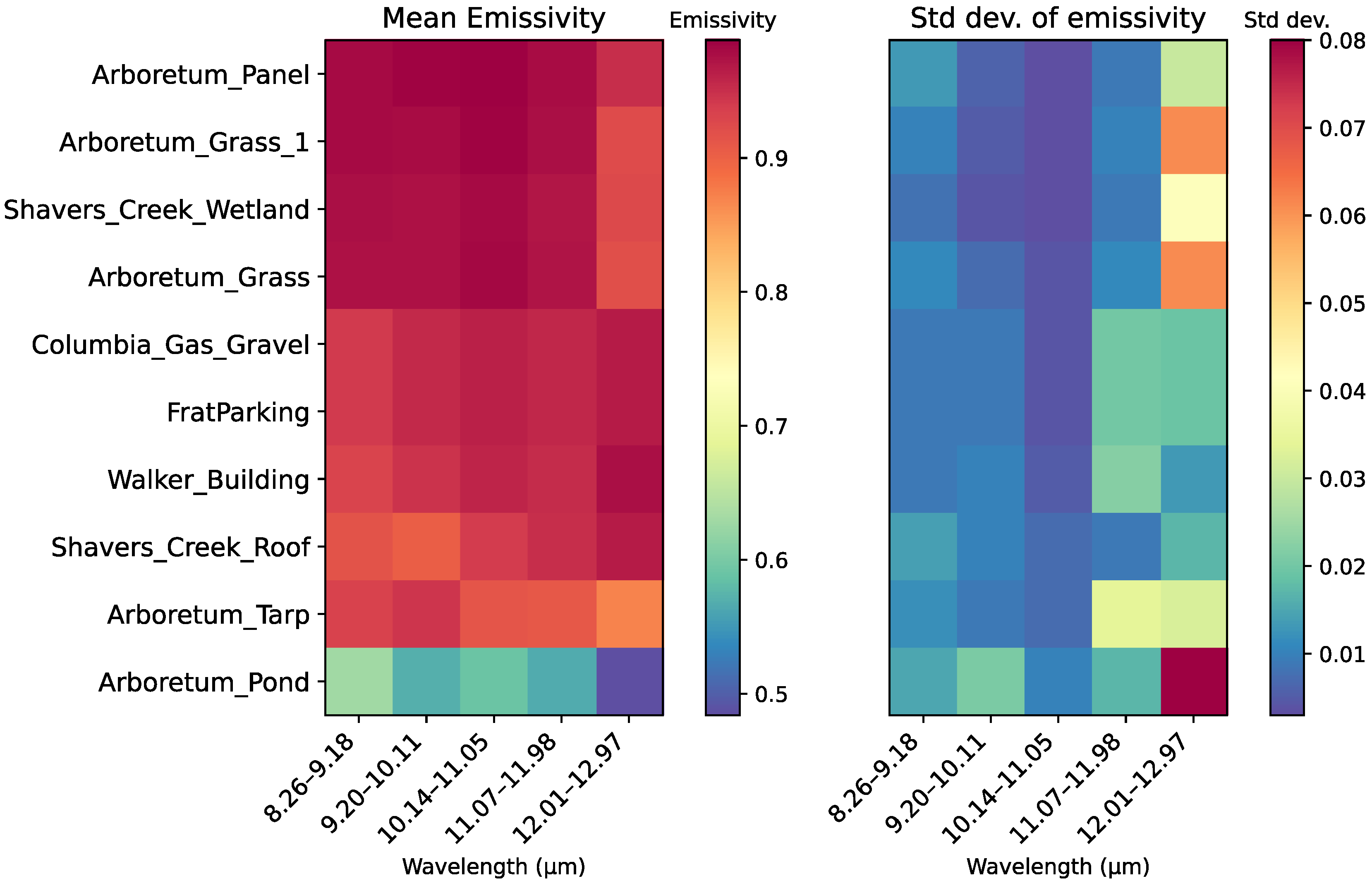
The spectral characteristics of target emissivity, partitioned into five equal wavelength intervals spanning 8.26–12.97 μm, revealed distinct patterns across different materials. As illustrated in Figure 11, emissivity values generally clustered between 0.8 and 1.0 for most targets, except for the Arboretum_Pond, which consistently displayed significantly lower values ranging from approximately 0.48 to 0.63 across all wavelength intervals.

The wavelength-dependent behavior of emissivity demonstrated notable trends. For all targets, the central spectral region (10.14–11.05 μm) exhibited the most stable emissivity values with minimal standard deviation (typically below 0.005 for most targets). This stability progressively diminished toward longer wavelengths, with the 12.01–12.97 μm interval showing substantially higher variability.

Table 4. Target emissivities averaged at the specific wavelength intervals (in μm), and corresponding standard deviation of the emissivity. Targets are ordered by their average emissivity.

Target Name	8.26–9.18	9.20–10.11	10.14–11.05	11.07–11.98	12.01–12.97
Arboretum panel	0.980 ± 0.013	0.985 ± 0.006	0.988 ± 0.003	0.977 ± 0.009	0.950 ± 0.030
Arboretum grass 1	0.980 ± 0.010	0.978 ± 0.005	0.986 ± 0.003	0.976 ± 0.010	0.922 ± 0.061
Shavers’ Creek wetland	0.975 ± 0.008	0.974 ± 0.004	0.979 ± 0.003	0.969 ± 0.009	0.924 ± 0.041
Arboretum grass	0.974 ± 0.011	0.973 ± 0.007	0.982 ± 0.004	0.971 ± 0.011	0.918 ± 0.061
Columbia Gas gravel	0.940 ± 0.009	0.953 ± 0.009	0.962 ± 0.004	0.956 ± 0.020	0.966 ± 0.019
Walker building roof	0.930 ± 0.009	0.946 ± 0.010	0.957 ± 0.005	0.951 ± 0.022	0.975 ± 0.013
Shavers Creek roof	0.914 ± 0.014	0.902 ± 0.010	0.938 ± 0.007	0.949 ± 0.009	0.965 ± 0.017
Arboretum tarp	0.932 ± 0.012	0.944 ± 0.009	0.912 ± 0.007	0.908 ± 0.034	0.868 ± 0.032
Arboretum pond	0.629 ± 0.015	0.569 ± 0.021	0.590 ± 0.010	0.565 ± 0.017	0.484 ± 0.080

quantifies these observations, with standard deviations in the longest wavelength interval reaching 0.080 for the Arboretum_Pond and 0.061 for both Arboretum grass samples, compared to values of 0.010 or less in the central spectral region.

This increased variability at longer wavelengths matches up with a strong atmospheric water absorption feature at about 12.6 μm. The strength of this absorption changes with viewing angle and distance in the MODTRAN simulations, adding more uncertainty to the emissivity retrievals at these wavelengths. This effect is most pronounced in the Arboretum_Pond target, where the cooler surface temperature (from the circulating cold water) results in weaker self-emission relative to atmospheric contributions. Even after atmospheric correction, the reduced signal-to-noise ratio for weak emitters makes the temperature-emissivity separation more sensitive to residual atmospheric uncertainties and calibration errors, particularly in spectral regions with strong atmospheric absorption.

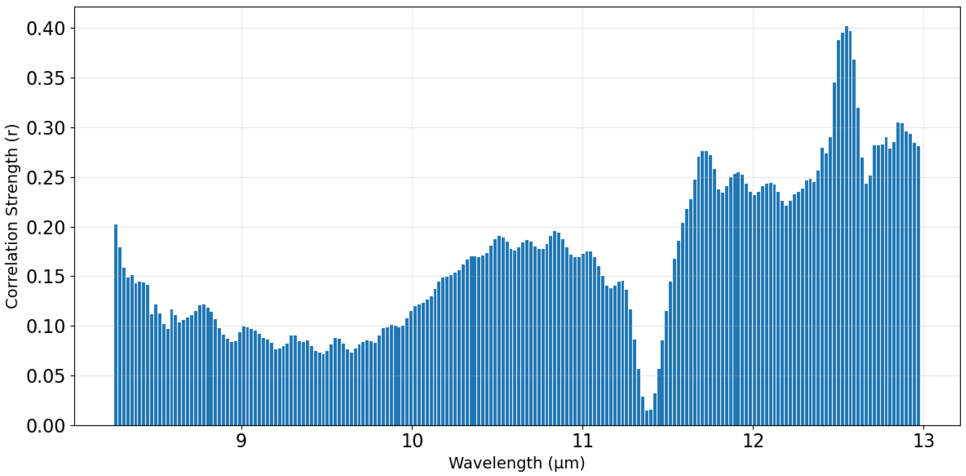
The relationship between viewing angle and spectral emissivity, shown in Figure 12, helps explain these wavelength-dependent variations. The correlation strength changes across the spectrum, with notably higher values in the 11.5–12.5 μm region where atmospheric absorption becomes more important. The clear peak at about 12.6 μm (reaching a correlation coefficient of 0.40) coincides with the water vapor absorption feature. This increased correlation in regions of strong atmospheric absorption suggests that emissivity retrievals become less reliable due to reduced signal levels, making it difficult to distinguish between genuine angular effects and measurement uncertainties introduced by the challenging atmospheric correction in this spectral region.

4.2. Emissivity Spectral Profiles

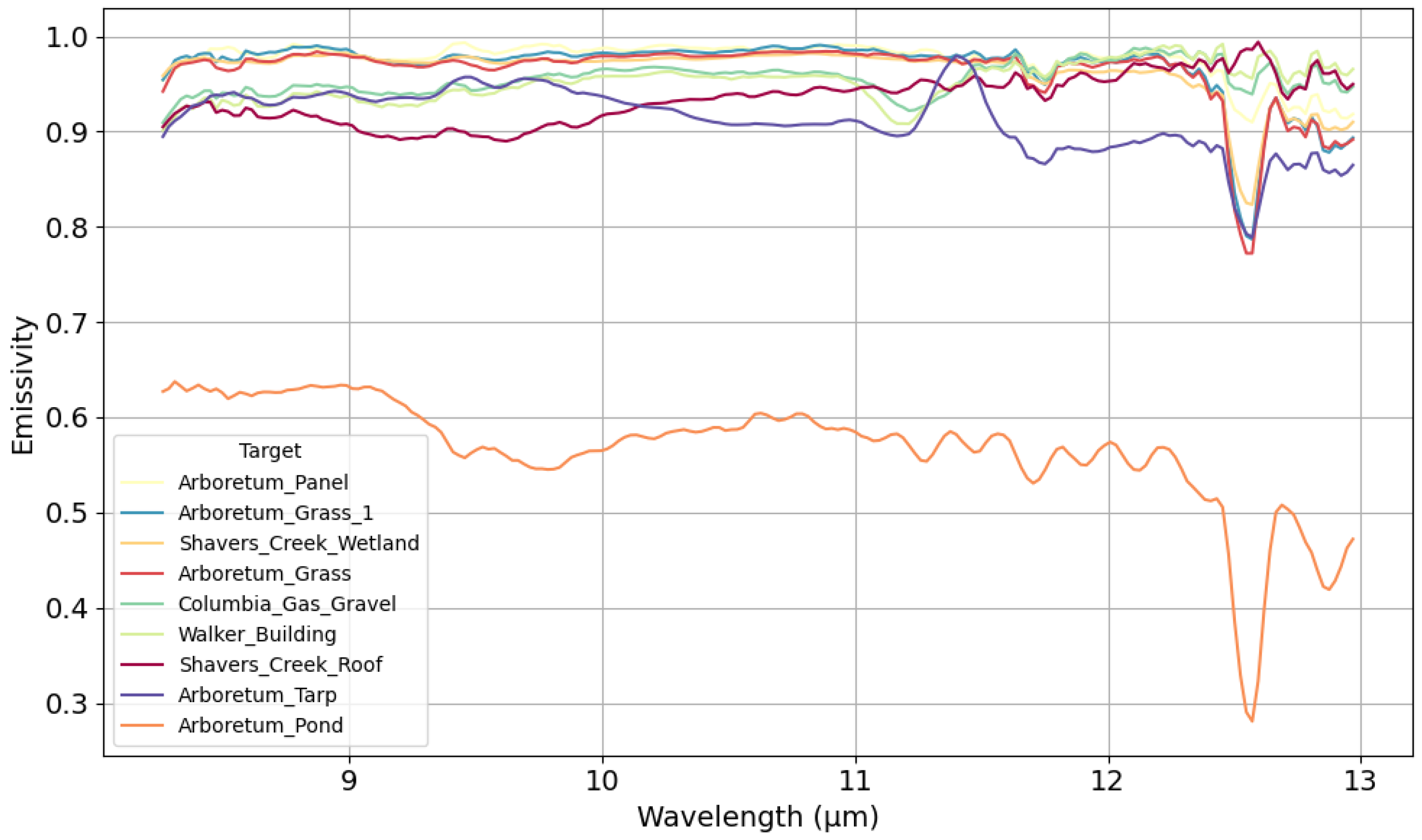
The emissivity spectra for each target, averaged across all pixels and viewing angles (Figure 13), show distinctive patterns. Most targets exhibit relatively smooth spectral profiles with gradual variations across the measured wavelength range. The natural surfaces (Arboretum_Grass, Shavers_Creek_Wetland) maintain consistently high emissivity values between 0.95 and 0.98 throughout most of the spectrum, with small decreases at wavelengths beyond 12 μm. The Arboretum_Pond target behaves very differently, with substantially lower emissivity (0.55–0.65) throughout the entire wavelength range and pronounced spectral features, including a significant dip to approximately 0.30 emissivity at 12.6 μm. This spectral pattern reflects the combined influence of the plastic material composition and the thermal properties of the cold circulating water. Another interesting spectral feature appears in the Arboretum tarp measurements, which shows a peak at approximately 11.4 μm that is absent in other targets. This spectral feature may represent a material-specific property, though its exact cause is uncertain without knowledge of the tarp composition. The common spectral feature observed across all targets is the pronounced emissivity drop at approximately 12.6 μm, which represents the atmospheric water vapor absorption band. The depth of this spectral drop varies among targets, with stronger effects in surfaces with lower overall emissivity, particularly the Arboretum_Pond.

4.3. Emissivity Distributions and Angular Dependence

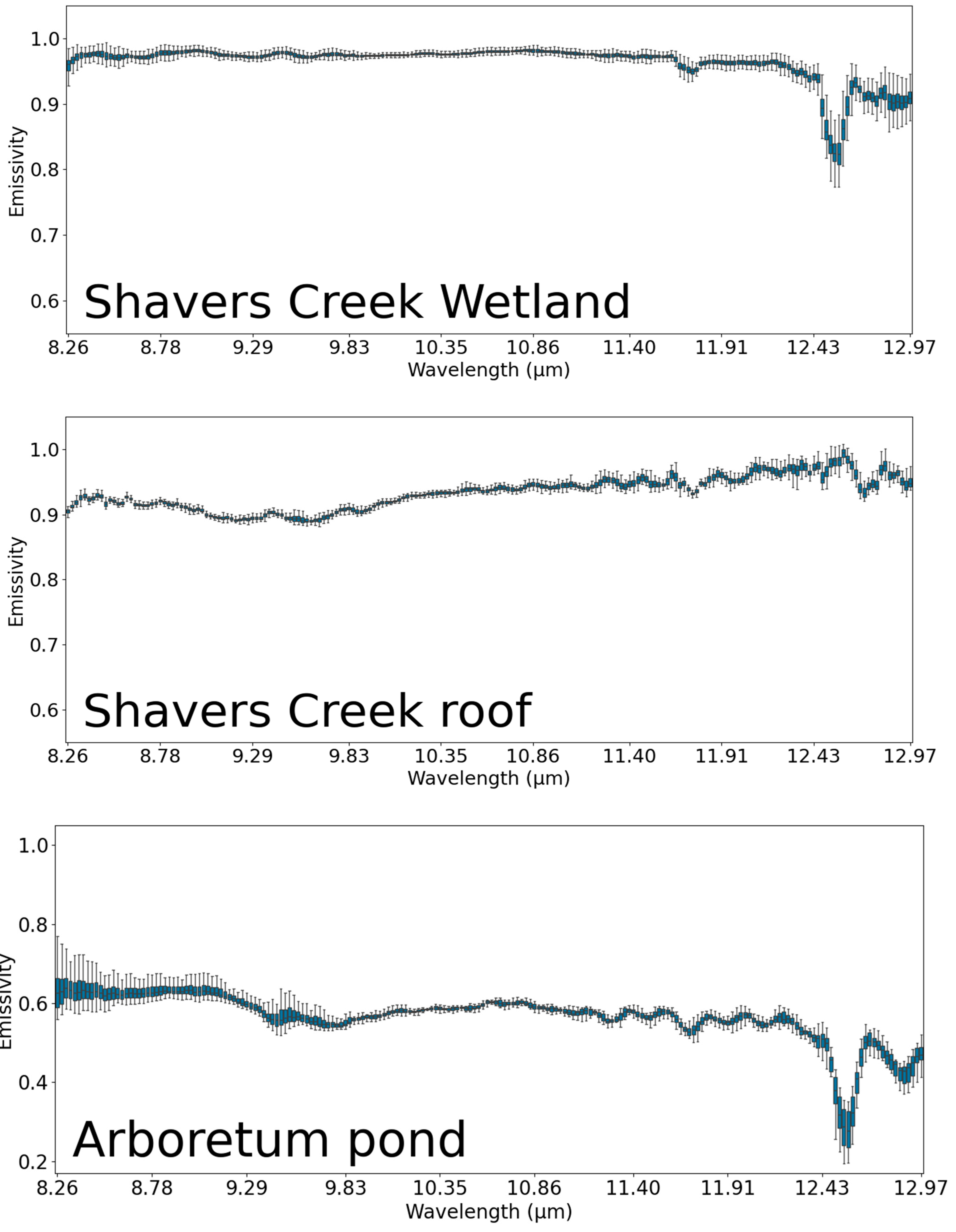
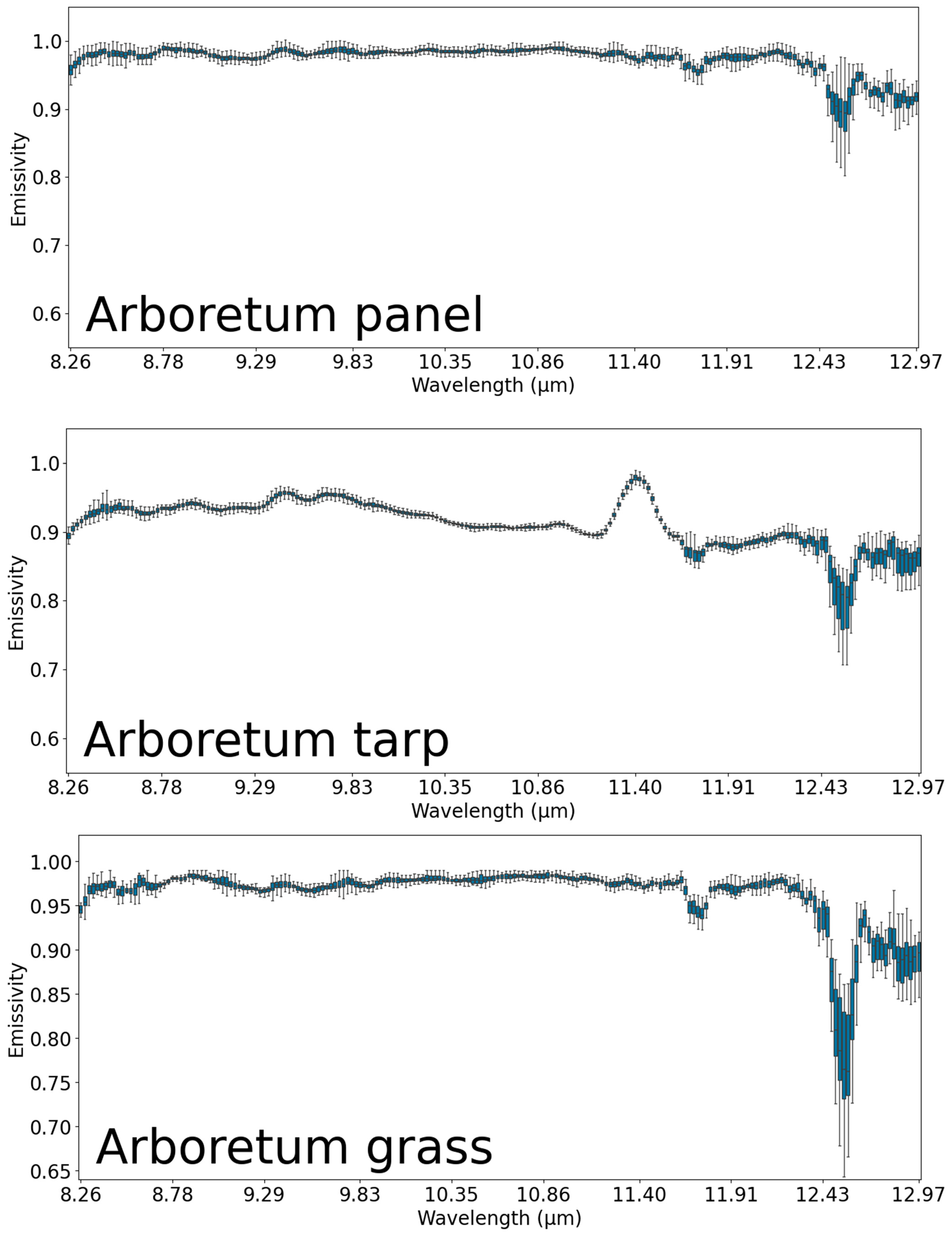
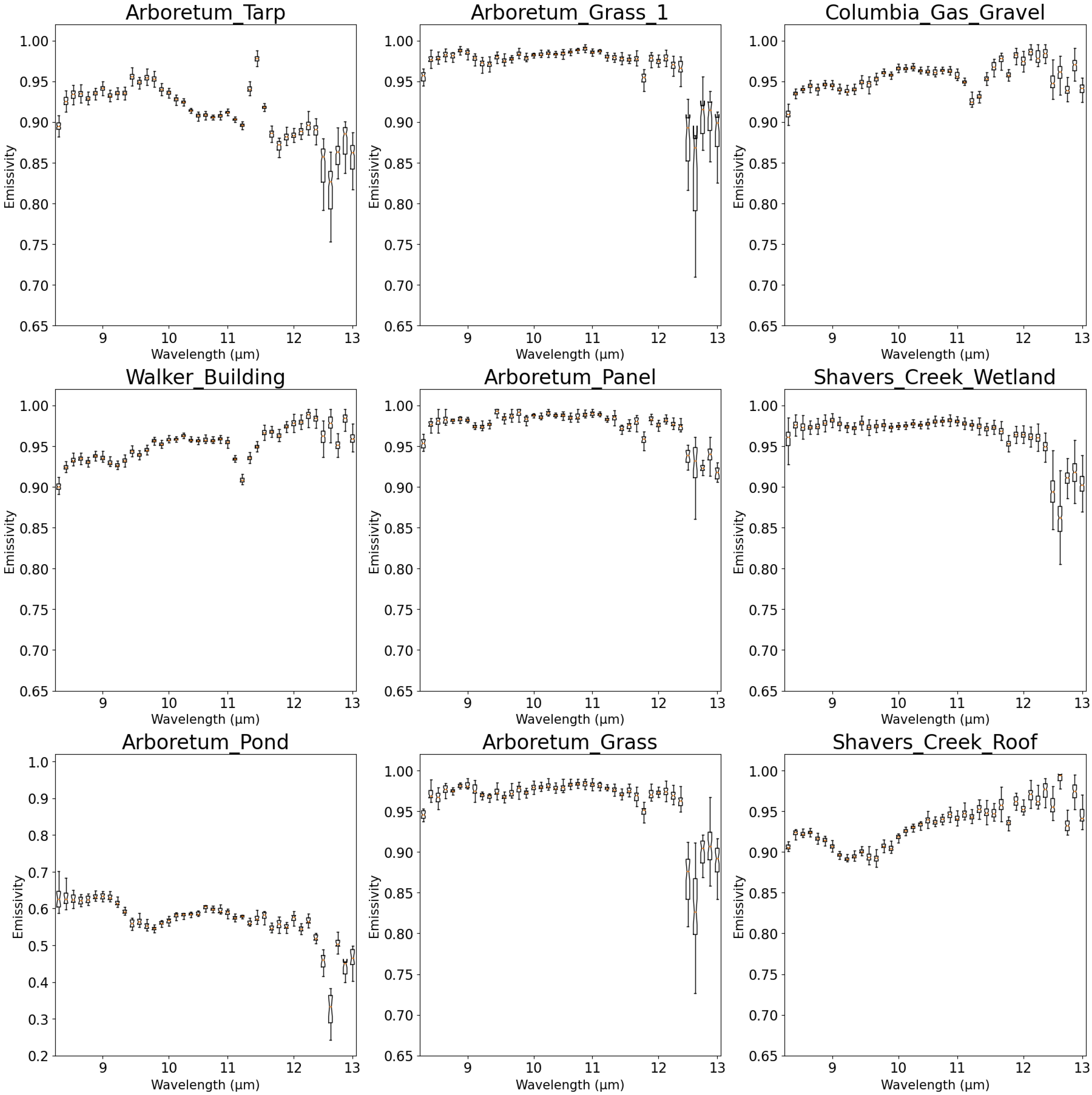
The statistical distribution of emissivity values, visualized through boxplots in Figure 14, demonstrates relatively compact spreads for most targets across most of the spectral range. A more detailed version of these boxplots is provided in Appendix B. The interquartile ranges typically span less than 0.05 emissivity units, indicating good measurement consistency despite variations in viewing angle and target heterogeneity. The increased variability in the 12–13 μm region reflects the fact that in spectral regions with strong atmospheric absorption, the retrieved values represent a mixture of residual atmospheric effects and true surface emissivity. The atmospheric correction becomes less reliable when the atmospheric path radiance dominates the surface-leaving radiance, leading to increased uncertainty in the temperature-emissivity separation.

Target-specific emissivity distributions reveal interesting patterns. The Arboretum_Pond exhibits the widest overall distribution, reflecting its complex thermal behavior resulting from the interaction between plastic material and cold water. Natural surfaces, particularly the grass samples, show extremely narrow distributions between 9 and 11 μm, indicating very consistent thermal emission properties across this spectral region regardless of viewing conditions.

The relationship between the emissivity and viewing angle, averaged across all spectral bands (Figure 15), reveals a consistent pattern across multiple targets. For surfaces with enough angular sampling range, emissivity stays relatively stable at viewing zenith angles between 40 and 50°, followed by a clear decreasing trend as the angle increases beyond 50°. This pattern holds true across different surface types, appearing in both high-emissivity natural targets (Arboretum_Grass varieties and Shavers_Creek_Wetland) and the low-emissivity Arboretum_Pond.

The amount of angle-dependent emissivity change varies among targets. The Arboretum panel and grass samples show modest decreases of about 0.003–0.008 emissivity units between 50° and 56° zenith angles, while the Arboretum_pond shows a more pronounced decrease of about 0.015 units over the same angular range, representing a proportionally larger effect given its lower overall emissivity.

Some targets, including Columbia_Gas_Gravel, Walker_Building, and Shavers_Creek_Roof, did not have measurements across a wide enough angular range to fully characterize their angular dependency. The available data for these targets is clustered within narrower angular ranges, preventing us from determining their emissivity behavior at more extreme viewing angles.

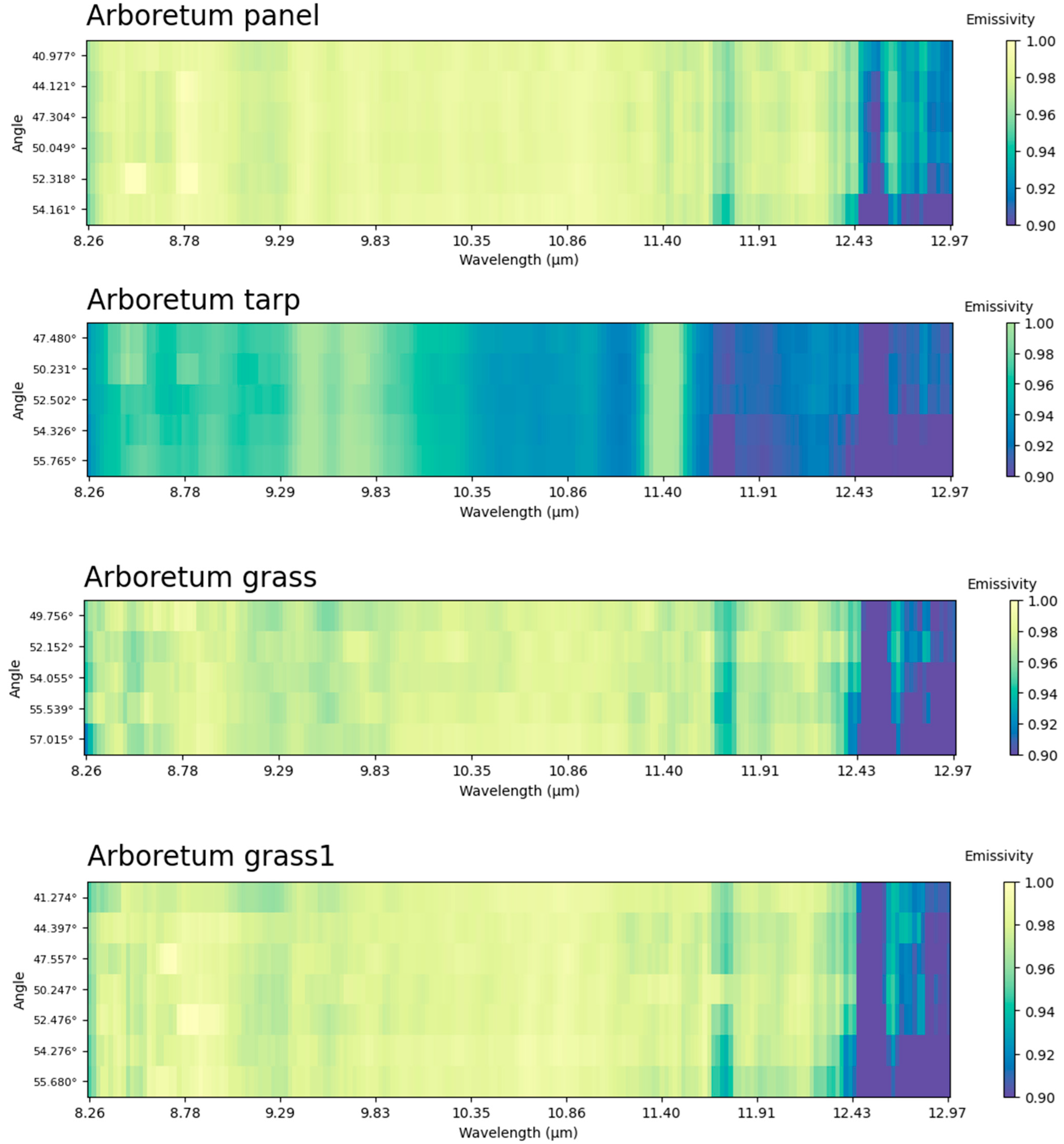
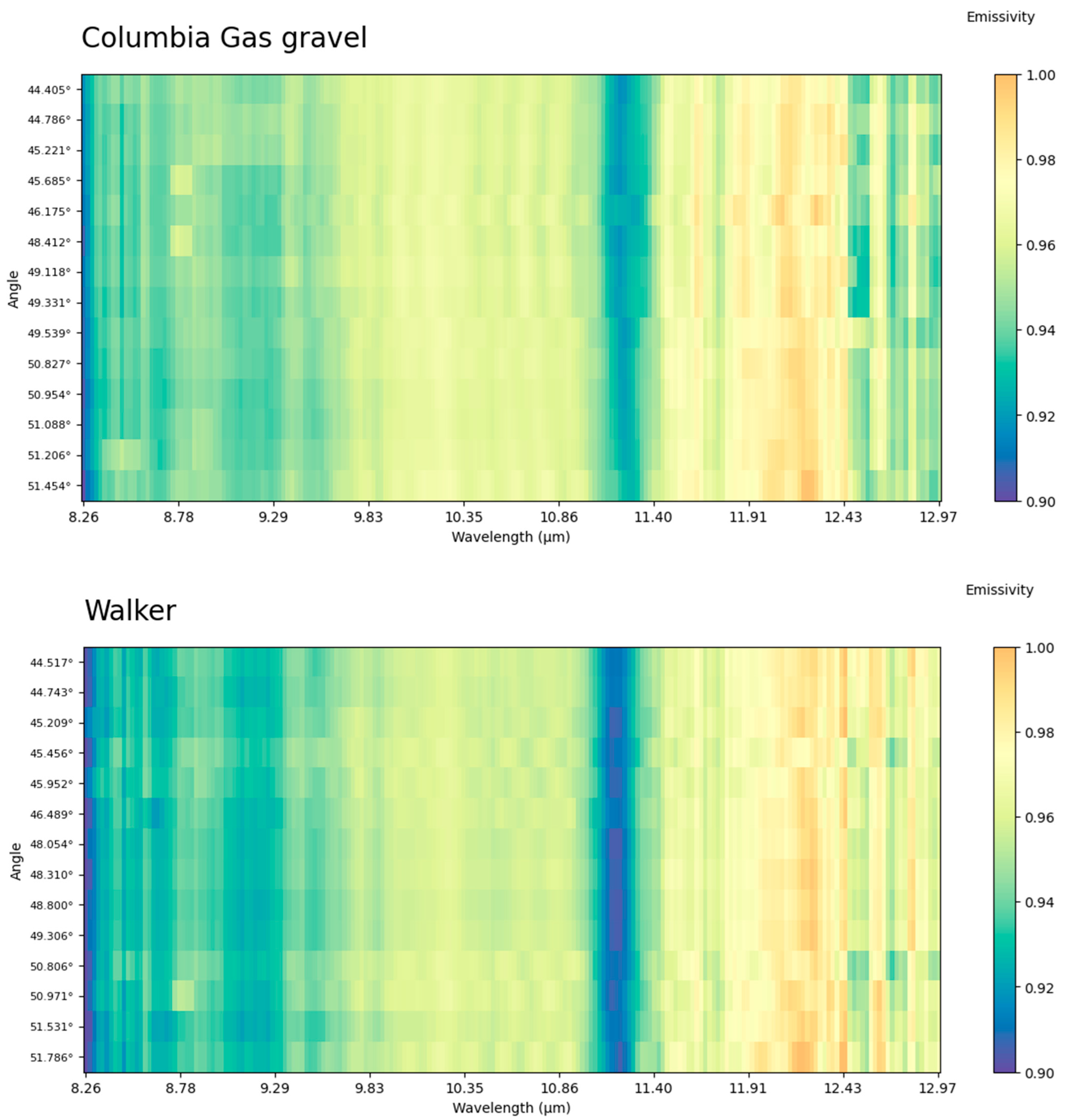
The observed angular dependency aligns with theoretical expectations based on Fresnel equations, which predict increasing reflectance (and thus decreasing emissivity) at larger viewing angles. This effect becomes particularly pronounced as viewing angles approach grazing incidence, though our measurements were limited to zenith angles below 56° due to practical constraints in the experimental setup. For more detailed plots, depicting angular and wavelength-dependent change in emissivity for different targets, refer to Appendix A.

The angular emissivity patterns observed in Figure 15 could provide an additional dimension for material discrimination. As proposed in [14] and suggested in [15], multi-angle observations can enable successful retrievals in non-optimal imaging conditions. Our results extend this by showing that different materials exhibit characteristic angular emissivity signatures. For instance, the Arboretum pond target shows a steeper angular decline in emissivity (0.015 units from 50 to 56°) compared to natural grass surfaces (0.003–0.008 units). These angular signatures could be incorporated into spectral libraries and classification algorithms to improve material identification accuracy.

5. Limitations

We were not able to precisely co-register images between batches using the SIFT (Scale Invariant Feature Transform) method. Co-registration within single batches had limited success. Images with distinct features (like the Walker building with numerous structures) yielded some control points, but alignment was imperfect when registering sequential images. Registering all images to the first image might have improved accuracy, but their overlap was too small for this approach. Registration failed completely for homogeneous scenes (like grasslands) due to a lack of distinctive features for tie points. However, recent advances in multimodal image registration based on structural similarity [38] and locally linear transformations [39] may offer some hope to these co-registration challenges in future work. This forced manual selection of pixels of interest between images. Another limitation was the imaging sensor re-calibrating between batches, preventing direct radiance comparison across batches. Since each batch contained few images, this resulted in a limited range of angles.

The atmospheric correction method also presented challenges. The model-based approach used first simulates atmospheric conditions through radiative transfer modeling, then applies derived profiles (transmission, upwelling, and downwelling) to remove atmospheric effects. This method is inherently limited without precise atmospheric data (such as radiosonde measurements taken during imaging), and even minor calibration discrepancies between the sensor and model can cause significant errors. In-scene atmospheric correction methods could be an alternative, as they determine atmospheric profiles directly from images. However, these methods (ISAC and similar approaches) cannot resolve downwelling radiation profiles and still depend on atmospheric transfer models (like MODTRAN) or empirical assumptions. Accurate downwelling characterization is essential for quantifying emissivity spectra of reflective surfaces.

The batch-to-batch calibration shifts limited our analysis. As shown in Figure 3, radiance differences between batches can exceed 10–15% for the same target, making direct comparison impossible without additional calibration procedures. This limitation forced us to analyze only images within single batches, which typically contained 5–14 overlapping images per target. Consequently, this reduced our angular coverage to approximately 8–15° ranges rather than the full 30° range that would have been possible using all available images across batches.

6. Conclusions

Viewing angle affects the appearance of the spectral targets in hyperspectral thermal imagery. In this study, we attempted to examine emissivity uncertainty in multi-angle LWIR hyperspectral data collected during the Nittany Radiance field experiment. Unlike previous research using model-based simulations or laboratory setups, this work utilized real-world airborne hyperspectral LWIR data captured from multiple viewing angles for different natural and man-made targets. Emissivity values remain relatively stable at viewing zenith angles between 40 and 50° but decrease consistently as angles exceed 50°. This angular dependency aligns with theoretical expectations from Fresnel equations, which predict increasing reflectance at larger viewing angles. Emissivity uncertainty varies significantly across the spectral range. The central spectral region (10.14–11.05 μm) is less variable with standard deviations typically below 0.005 for most targets. Variability increases significantly in regions with strong atmospheric absorption features, particularly around the water vapor band at 12.6 μm, where residual atmospheric effects contaminate the retrieved emissivity values. This limitation indicates that emissivity retrievals in the 12–13 μm spectral region should be interpreted with caution or excluded from analysis. Natural surfaces demonstrated high and consistent emissivity values (typically 0.95–0.98), with grass, wetland, and gravel targets showing minimal variability across most of the spectrum despite changes in viewing angle. Man-made targets displayed greater variability, with the Arboretum Pond exhibiting lower emissivity (0.55–0.65) and stronger spectral features.

We addressed technical challenges in multi-angle atmospheric correction, such as developing a modified atmospheric correction method adapted from FLAASH-IR for multi-angle scenarios. This approach generated angle-specific atmospheric profiles that account for varying path lengths and angles with a change in the viewing geometry. Limitations remain in precise image co-registration within a single image acquisition batch as well as between batches. Accurate atmospheric parameter estimation is also problematic without available radiosonde atmospheric soundings. The findings suggest that measurements in the 10–11 μm wavelength range and viewing angles below 50° provide maximum stability of the resolved material emissivity. The conventional assumptions of Lambertian behavior for natural surfaces hold reasonably well within limited angular ranges but break down at more extreme viewing angles.

Future research should focus on parabolic flight routes with rotating wing aircraft, such as helicopters or small UAVs, to maintain constant distance while varying imaging angles. This approach would simplify atmospheric correction by eliminating range variation as an unknown factor while expanding the angular measurement range. Scene-based correction methods like Oblique ISAC offer alternatives to model-based atmospheric correction approaches. They are still relying on the radiative transfer models for the scaling of the resolved radiance spectra to the correct physical units, but promise to resolve the shape of the atmospheric profiles more accurately. Image co-registration between batches could benefit from modern AI-based registration techniques, eliminating the need for manual pixel sampling. The observed spectral and angular dependencies could enhance material classification algorithms by incorporating multi-angle information as a discriminative feature rather than treating it as measurement noise.