Article

Marginal Contribution Spectral Fusion Network for Remote Hyperspectral Soil Organic Matter Estimation

by
Jiaze Tang
1,
Dan Liu
1,
Qisong Wang
1,*,
Junbao Li
2,
Jingxiao Liao
3 and
Jinwei Sun
1
1
Electrical Measurement Technology and Intelligent Control Institute, School of Instrumentation Science and Engineering, Harbin Institute of Technology, Harbin 150080, China
2
A Information Countermeasure Technique Institute, School of Computer Science and Technology, Harbin Institute of Technology, Harbin 150080, China
3
Department of Industrial and Systems Engineering, The Hong Kong Polytechnic University, Hung Hom, Kowloon, Hong Kong
*
Author to whom correspondence should be addressed.
Remote Sens. 2025, 17(16), 2806; https://doi.org/10.3390/rs17162806
Submission received: 18 June 2025 / Revised: 7 August 2025 / Accepted: 10 August 2025 / Published: 13 August 2025

Abstract

Soil organic matter (SOM) is a fundamental indicator of soil health and a major component of the global carbon cycle; its accurate quantification is essential for sustainable agriculture. Conventional chemical assays yield only point-based soil measurements and miss the spatial distribution of soil elements; airborne hyperspectral remote sensing has emerged as a promising approach for the quantitative measurement and characterization of SOM. Inversion models translate hyperspectral data into quantitative SOM estimates. However, existing models rely solely on a single preprocessing pathway, limiting their ability to fully exploit available spectral information. We address these limitations by developing a marginal contribution-driven spectral fusion network (MC-SFNet) that conducts feature-level fusion of heterogeneous preprocessing outputs within a physics-guided deep architecture. Moreover, the combination of data-driven fusion and the Kubelka–Munk (KM) model yields more physically interpretable spectral features, advancing beyond prior purely data-driven methods. We validated MC-SFNet on a self-constructed remote sensing, high-throughput hyperspectral dataset comprising 200 black soil samples from Northeastern China (400–1000 nm, 256 bands). Experimental results show that our network reduces the RMSE by 10.7% relative to the prevailing generalized hyperspectral soil-inversion model. The proposed method provides a novel preprocessing pathway for forthcoming airborne high-throughput hyperspectral missions to extract soil-specific spectral information more effectively and further enhance large-scale SOM retrieval accuracy.

1. Introduction

Soil is a fundamental resource for agricultural production, and its quality directly influences the sustainability of agricultural practices and the protection of the ecological environment [1,2]. Among various soil attributes, soil organic matter (SOM) content is a key indicator of soil fertility, microbial activity, and overall environmental function [3,4,5,6]. Accurate and rapid assessment of SOM is particularly important for precision agriculture, as improper fertilization, whether excessive or insufficient, can lead to suboptimal crop yields and negative environmental impacts. Therefore, accurate and timely measurements of soil fertility are crucial for ensuring that fertilizers are applied in the right amounts, optimizing agricultural productivity, and minimizing the adverse effects of over-fertilization or under-fertilization on the environment [7]. Emerging remote-sensing techniques, especially high-throughput hyperspectral imaging, offer a viable route to invert spatially continuous SOM information from field to regional scales [8]. Inversion methods, which utilize spectral data, provide an efficient way to estimate SOM content across large areas. When these subtle spectral signatures are regressed against laboratory-measured samples using multivariate calibration or modern machine learning techniques, up to 80% of the variance in SOM content can be explained under controlled conditions [9]. This laboratory relationship is scalable: an airborne hyperspectral imager, when combined with a regional soil spectral library, produced 1 m resolution maps of SOM stock in Italy’s Sele River Plain [10], while Unmanned Aerial Vehicle (UAV) hyperspectral cubes, calibrated with only twenty soil samples, achieved 1 m resolution field-scale SOM predictions, far surpassing the accuracy of ordinary kriging interpolation [11].
Spaceborne imaging spectrometers have extended this capability from small plots to large regions: a meta-learner improved prediction accuracy for Moroccan croplands by approximately 48.8% compared to individual models like Random Forest, Support Vector Regression, and PLSR. The model’s coefficient of determination, R2, reached 0.65, with an RMSE of 0.194% and an RPIQ of 2.247 [12]. The first evaluation showed that selecting thirty standard normal variate-corrected bands for 282 samples yielded more accurate results, with R2 increasing to 0.68 and RMSE decreasing to 0.34%, compared to the original full-band model, which had an R2 of 0.60 [13]. China’s GF-5 imagery, after waveletpacket denoising, achieved similar accuracies for SOM mapping at a 30 m resolution, with R2 increasing from 0.62 to 0.77 after applying wavelet denoising and further improving to 0.84 with 0.6-order wavelet denoising, while RMSE decreased by 0.84 g·kg−1 [14]. Meanwhile, tractor-mounted spectrometers adapted to Brazilian Cerrado soils by locally adjusting their calibration sets [15]. Combined hyperspectral analyses of gypsum-rich terrains show that spectral indices with machine learning can simultaneously estimate SOM and distinguish interfering minerals, paving the way for scalable, cloud-based continental-scale digital soil-mapping pipelines [16]. Consequently, quantitative inversion of SOM using hyperspectral data has become a burgeoning area of research in soil science [17,18,19,20,21].
Initial studies predominantly employed linear models, such as partial least squares regression (PLSR), for modeling soil hyperspectral data [22]. For example, Shi [23] successfully utilized PLSR to predict soil total nitrogen content. However, as the field matured, nonlinear approaches gained prominence. Machine learning methods, such as Support Vector Machines (SVMs) and Random Forest (RF), have been shown to outperform traditional linear regressions in hyperspectral SOM estimation. Feng et al. [24] achieved superior results by applying SVM and Random Forest to invert soil arsenic content from hyperspectral data, and other studies have also demonstrated that Random Forest often provides higher accuracy in estimating SOM and soil moisture [25]. Similarly, Chung [26] applied a RF model to invert soil mercury content from hyperspectral data, while Subi [27] employed PLSR to predict chromium in arid zone.
More recently, deep learning techniques have been introduced into the field of SOM inversion. Their capacity to model complex nonlinear relationships and handle large-scale datasets has made them particularly attractive [28]. Kawamura et al. [29] proposed a convolutional neural network (CNN)-based method to estimate phosphorus, while Wang et al. [30] integrated deep learning approaches to predict soil moisture from hyperspectral data. Li et al. [31] employed a 1D CNN to classify soil texture, and Cao et al. [32] used a deep CNN to predict soil organic matter. Ajay [33] leveraged deep learning to analyze hyperspectral data for total soil nitrogen prediction. Collectively, these efforts illustrate the potential of deep learning to improve the accuracy and efficiency of hyperspectral inversion for soil properties, inspiring new directions in precision agriculture and soil quality assessment.
Many studies have also explored hyperspectral data preprocessing strategies to optimize inversion performance [34] further. Zhang [35] demonstrated that first-order derivative preprocessing can effectively highlight key information in soil spectra. At the same time, Jiachen [36] identified standard normal variate (SNV) as the most suitable preprocessing method for hyperspectral soil inversion. In contrast, X. B. [37] argued that deep learning, such as CNNs with end-to-end architectures, can eliminate the need for explicit preprocessing.
Despite these advances, understanding of inverted SOM in hyperspectral wavelengths under different preprocessing methods is still limited. To address this gap, we therefore extend the marginal contribution feature importance (MCI) [38] paradigm, constructing a bespoke analysis that tracks wavelength-wise marginal gains under varied treatments and underscoring the risk of relying on any single treatment.
This paper makes three primary contributions: (1) We introduce a wavelength-wise, marginal contribution framework that quantifies the predictive value of every spectral band under each preprocessing operator, producing an interpretable importance map for band selection and computational pruning; (2) we develop a hybrid preprocessing scheme that couples the Kubelka–Munk (KM) optical model with data-driven treatments, yielding features linked to intrinsic absorption while retaining the multivariate structure of reflectance, thereby enhancing physical interpretability; (3) we propose a physics-guided deep network that performs feature-level fusion of heterogeneous preprocessing outputs. Fusion weights are initialized from the marginal contribution scores and refined end-to-end, overcoming the limitations of single-preprocessing pipelines and enabling higher accuracy with fewer, more informative bands.

2. Proposed Method

The overall workflow of this study is illustrated in Figure 1. The research procedure includes the following steps: (1) collecting 200 black soil samples at 45.74°N, 127.39°E in Northeastern China; (2) acquiring the original soil spectra and measuring the SOM content using the potassium dichromate volumetric method; (3) applying various preprocessing methods to the soil spectral data; (4) conducting marginal contribution analysis of different preprocessing strategies using the marginal contribution approach within a unified framework; (5) the design of a marginal contribution-driven spectral fusion network (MC-SFNet) architecture for the inverse regression of soil spectra.

2.1. Spectral Preprocessing

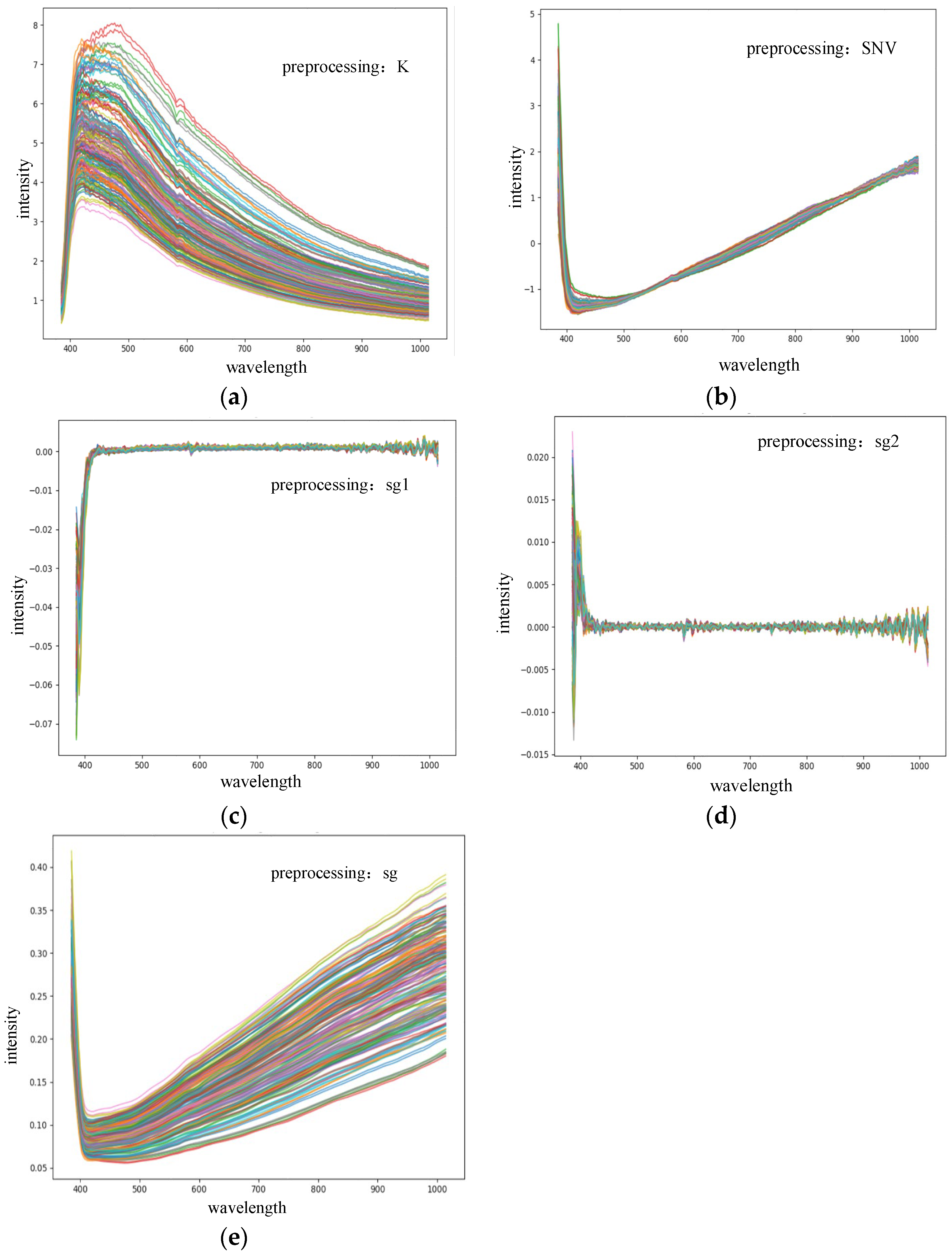
To highlight spectral features and reduce noise, the MC-SFNet integrates several preprocessing methods usually used in contemporary studies [23,24,34,36], with their visualizations shown in Figure 2. Savitzky–Golay (SG) [39] Filter: Smooths and differentiates the original spectra to reduce high-frequency noise while preserving key spectral features. First-Order Derivative (SG1) [40]: Calculates the first-order difference in the spectral signals to emphasize absorption wavelength edges and mitigate systematic errors caused by background shifts. Second-order Derivative (SG2): Further enhances subtle absorption features while reducing nonlinear background interference. SNV [41]: Corrects spectral amplitude variations due to differences in particle size, surface roughness, and scattering, ensuring greater comparability in spectral amplitude and scale. In addition to the data-driven preprocessing methods, this study incorporates the Kubelka–Munk soil spectral model as a physical preprocessing approach [42], enabling the integration of data-driven and physical-modeling-based preprocessing. Kubelka–Munk (KM) Transformation: Converts soil reflectance data into absorption coefficients (K values) using the Kubelka–Munk model to relate the spectral data more closely to intrinsic optical properties, thereby improving the interpretability and stability of SOM inversion.
The KM model, introduced by Kubelka and Munk in 1931 [42], relies on two key assumptions: (1) light propagates only forward and backward within the material, and (2) the material is homogeneous at a macroscopic scale. Using the KM model, reflectance (R) is transformed into the absorption coefficient (K) in Equation (1).
K = ( 1 R ) 2 2 R
In this study, the MC-SFNet integrates both data-driven preprocessing and the KM physical model. First, multiple preprocessing steps generate a diverse set of spectral features. Then, the KM model is applied to compute the K, which is fused with the preprocessed reflectance data to form feature sets that are richer and more physically meaningful. This hybrid strategy retains the multivariate feature information inherent in the spectral data, while the incorporation of the KM model enhances interpretability.

2.2. Unified Permutation–Gain Analysis for Multi-Preprocessed Spectra

In practical soil spectroscopy applications, strong inter-band collinearity produces substantial wavelength redundancy; this not only enlarges the feature space and elevates on-board computational cost, but can also induce a slight accuracy decline when the estimator is over-parameterised [43,44,45]. Existing band reduction studies typically mitigate redundancy by running a single preprocessing route and then clustering the spectra—K-means, spectral clustering or similar—to keep one representative wavelength per cluster [46,47,48]. Although these unsupervised heuristics offer only coarse dimensionality control, they still fail to clarify how individual bands affect inversion accuracy and provide no physical interpretability, thereby constraining subsequent model extensibility [49].
Because the MC-SFNet architecture concatenates K heterogeneous preprocessing streams, the effective number of input channels grows from N to KN; redundancy is therefore magnified rather than suppressed. To address this issue, we introduce a marginal contribution permutation–gain analysis that assigns an explicit importance score to every “preprocess-band” pair and enables fine-grained pruning before the network is deployed. MCI overcomes the limitations of traditional importance measures such as Shapley-value-based methods [50] and mitigates covariance-induced attribution bias among correlated features.
Let R = r m n M × N denote the matrix of raw bidirectional reflectance, where M is the number of soil samples and N indexes the discrete wavelengths between 400 nm and 1000 nm. Consider a set of K complementary preprocessing operators P 1 , , P K in Equation (2). Applying each operator independently to R yields the following:
X ( k ) = P k ( R ) M × N , k = 1 , , K
And concatenating these matrices along the spectral dimension produces X in Equation (3).
X = X ( 1 ) | | X ( K ) M × D , D = K N
Let y = y 1 , , y M be the chemically determined SOM vector. A one-dimensional convolutional regressor g θ : D is trained by minimizing the empirical mean-square error in Equation (4).
θ = arg min θ 1 M M m = 1 g θ x m y m 2
with x m denoting the m-th row of X .
The resulting baseline error over the complete feature set F = { 1 , , D } is as in Equation (5).
v 0 = 1 M M m = 1 g θ x m y m 2
To quantify the contribution of an individual feature j F , introduce a permutation operator Π j that randomly shuffles column j across the sample dimension while keeping all other columns intact. Π j , p is a permutation drawn uniformly at random from the symmetric group on M elements. For the p-th independent permutation, the prediction error becomes the quantity in Equation (6).
v j , p = 1 M M m = 1 g θ Π j , p x m y m 2 , p = 1 , , P
where P denotes the number of repetitions. Because the permutation disrupts the statistical dependence between feature j and the target, one necessarily has v j , p v 0 .
Averaging the error increments over all permutations defines the permutation–gain score in Equation (7).
I j = 1 P P p = 1 v j , p v 0 0
which serves as an unbiased Monte Carlo estimate of the marginal predictive value of feature j while requiring only a single model fit. Index j can be uniquely decomposed as j = ( k 1 ) N + n with k { 1 , , K } and n { 1 , , N } .
Collecting these scores produces the importance matrix in Equation (8).
I = I 1 , 1 I 1 , N I K , 1 I K , N K × N
whose (k,n)-th entry reflects the independent gain obtained by injecting wavelength λ n after preprocessing route P k . Equation (8) therefore delivers a fully quantified importance landscape spanning all preprocessing streams and spectral channels; this matrix simultaneously provides the ranking basis for wavelength selection and supplies the prior weight initialization for the subsequent spectral fusion network.

2.3. Marginal Contribution-Driven Spectral Fusion Network

To optimally integrate multiple preprocessing pathways into a unified network that is informed by both data-driven and physics-based models, we propose two complementary approaches for spectral fusion: MC-SFNet-WIN (wavelength-level integration) and MC-SFNet-FIN (feature-level integration). Both architectures employ a lightweight 1D-CNN [51] backbone for feature extraction and dimensionality reduction, with the primary difference lying in how the spectral features are fused—at the wavelength level in MC-SFNet-WIN and at the feature level in MC-SFNet-FIN.
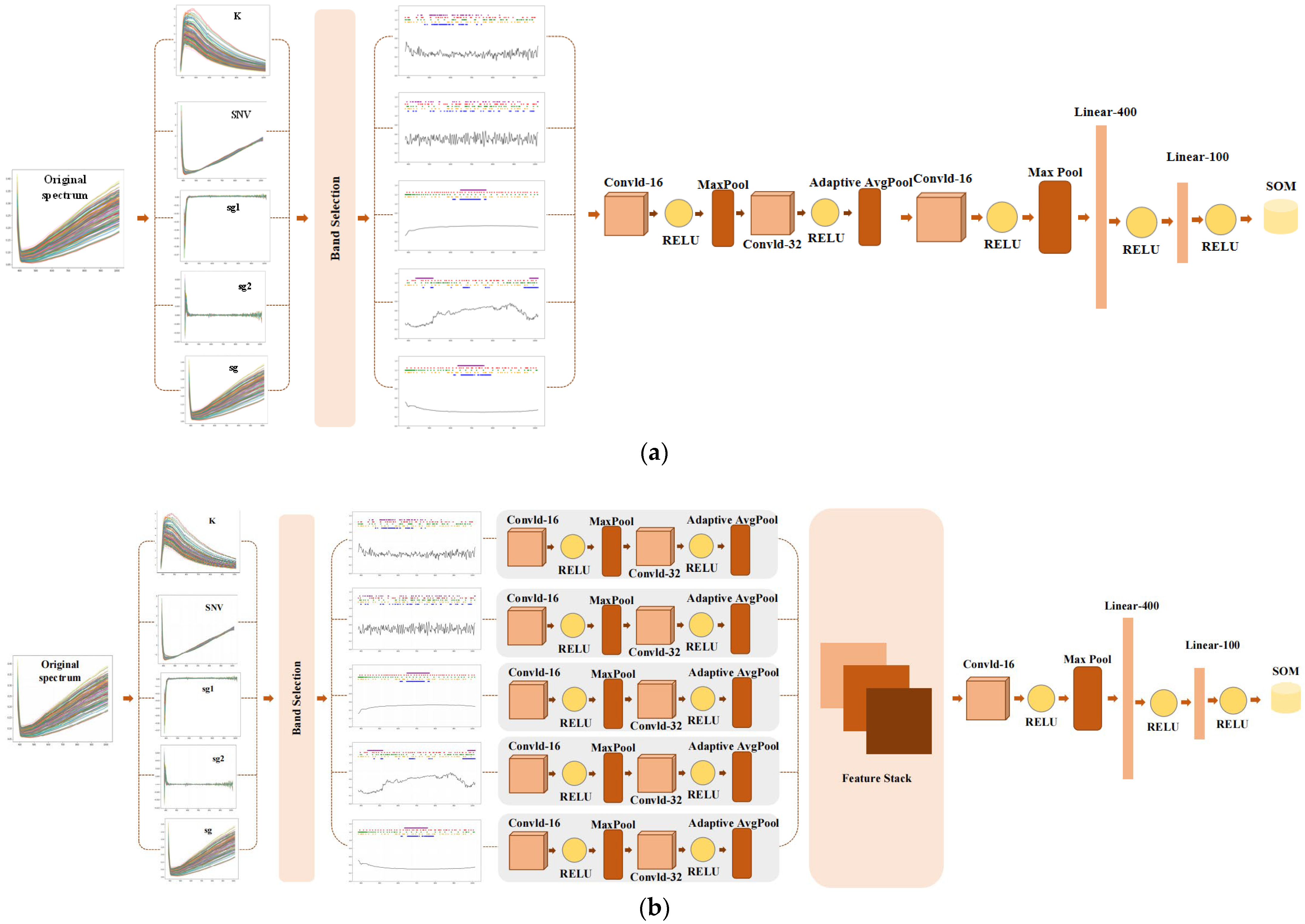
In the MC-SFNet-WIN approach, the raw spectral data, denoted as R = r m n R M × N , where M represents the number of soil samples and N corresponds to the number of spectral bands, is processed through K complementary preprocessing operators P 1 , P 2 , , P K . These preprocessing methods include standard approaches like SG, SG1 and SG2, SNV, and the KM physical model. After applying these operators, each produces a preprocessed spectral matrix. This integrated feature set is then used as an input to MC-SFNet for modeling in Figure 3a, where the marginal contribution importance analysis plays a crucial role in selecting the most relevant spectral bands.
First, the MC-SFNet extracts a feature subset from the original spectral data based on marginal contribution. This subset is then passed through the 1D-CNN, which consists of two convolutional layers (with 16 and 32 kernels, respectively, and a kernel size of 3) and corresponding pooling layers. These layers capture multiscale spectral information through hierarchical feature extraction and dimensionality reduction [52]. After concatenating the output feature vectors from all branches, a global convolutional layer (16 kernels) and subsequent max-pooling further compress and refine the features. Finally, the fused features are passed through a fully connected network with one hidden layer (100 ReLU-activated neurons) and a linear output layer, enabling SOM content prediction.
In contrast, the MC-SFNet-FIN approach processes each preprocessing stream independently at the feature level. In this case, each preprocessed spectral matrix X is passed through a shallow 1D-CNN to generate compact feature vectors for each preprocessing method in Figure 3b. The resulting features are then combined using a multi-head weighting block, where the weights for each feature are initialized based on the previously computed MCI scores and refined during training. This fusion strategy ensures that the most significant spectral features, as identified through MCI, are given more weight in the final prediction.
The aggregated feature vector, which combines information from all preprocessing methods, is passed through a fully connected network to predict the SOM content. The key difference between MC-SFNet-WIN and MC-SFNet-FIN lies in the way features are combined: the former fuses at the wavelength level, while the latter operates at the feature level, allowing for a more flexible fusion mechanism.
One of the unique aspects of our approach is the inclusion of the KM model in the preprocessing stage. The KM transformation, as previously defined in our formula, relates the spectral reflectance data to absorption coefficients. This physical preprocessing step enhances the interpretability of the model by ensuring that the spectral features are not only statistically relevant but also physically meaningful. Specifically, the transformation from reflectance to absorption using the Kubelka–Munk model facilitates a more direct link between the spectral data and the intrinsic properties of the soil. This fusion of data-driven and physical models contributes to the robustness and stability of the spectral inversion process.
Finally, the deep learning model is trained to minimize the error in predicting the SOM content. The training process is based on minimizing the empirical mean-square error θ * This approach ensures that the model learns to predict SOM content with high accuracy.
In summary, the MC-SFNet-WIN and MC-SFNet-FIN architectures, through the integration of multiple preprocessing streams and the application of marginal contribution-driven feature selection, provide a powerful framework for the inversion of SOM from hyperspectral soil data. By combining data-driven machine learning techniques with physics-based models like Kubelka–Munk, we achieve a robust and interpretable solution for large-scale soil mapping. The use of marginal contribution analysis for feature selection and the incorporation of a 1D-CNN backbone allows for the efficient extraction of relevant spectral features, leading to improved SOM estimation accuracy.
The MC-SFNet network architecture is detailed in Table 1, with the following layer specifications. In Table 1, the parameters are defined as follows: batch_size refers to the number of samples processed in each training step, preprocess indicates the preprocessing method applied to the data, features corresponds to the number of spectral bands or input features, and global_output is the output size of the Global Conv1d layer, set to 128 in this model. These parameters determine the dimensions of the input and output at each layer, ensuring proper data flow and model functionality.

3. Experiments

3.1. Experimental Settings

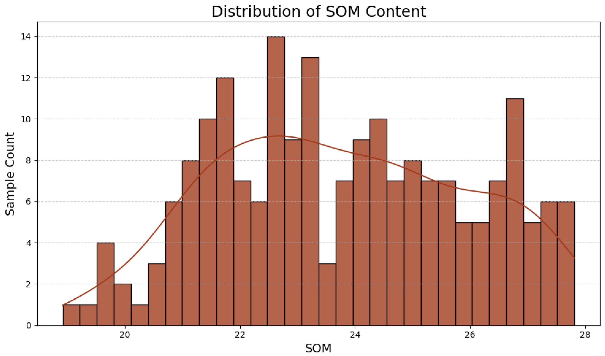
As shown in Figure 4, our team previously collected 200 black soil samples as part of a prior study conducted in Northeastern China at the coordinates 45.758°N to 45.772°N and 127.39°E to 127.40°E. Sampling took place across two agricultural fields in the region, with 100 samples collected from each field. The samples were arranged in a 10×10 grid, with each sampling point spaced 15 to 20 m apart. At every point, soil samples were gathered from five cores—four positioned at the corners and one at the center of a 2 m by 2 m area, all spaced more than 1 m apart—and subsequently mixed [4]. In Figure 5, the statistical characteristics of the SOM content are summarized: the mean is 23.77 g kg−1, with a standard deviation of 4.75 g kg−1, a maximum of 27.81 g kg−1, and a minimum of 18.92 g kg−1. The y-axis represents the number of soil samples in each category. To ensure objective and reliable results, the 200 soil samples were randomly divided into five folds for cross-validation. Soil spectral cubes were collected with a GaiaField Pro-V10 push-broom hyperspectral imager (400–1000 nm, 256 bands, 3.5 nm resolution). Because this instrument captures spatially contiguous hyperspectral images in a single scan, it delivers high-throughput, imaging-based data rather than the point measurements produced by traditional non-imaging spectrometers, thereby closely emulating the data characteristics of airborne hyperspectral remote-sensing platforms and providing a more realistic test bed for SOM-inversion algorithms.

3.2. Evaluation Criteria

To assess the performance of SOM inversion using corrected spectra, this study employed three indicators: the coefficient of determination (R2) [53], the root mean square error (RMSE), and the Pearson correlation coefficient (PCC) [54]. Among these, R2 measures the goodness of fit between predicted and observed values, ranging from 0 to 1, with values closer to 1 indicating higher predictive accuracy. Let y denote the observed values, ŷ the predicted values, and y ¯ the mean of the observed values; the formula for R2 is defined as Equation (9):
R 2 = 1 ( y y ^ ) 2 ( y y ¯ ) 2
The RMSE is calculated as Equation (10):
R M S E = 1 n n i = 1 y i y ^ i 2
In addition, the PCC quantifies the linear correlation between predicted and observed values. Its range extends from −1 to 1, where larger positive values indicate stronger positive correlations. By employing these three metrics—R2, RMSE, and PCC—this study comprehensively evaluates the model’s performance in SOM inversion [44].

3.3. Interpretation of Wavelength Marginal Contributions

Previous research on soil hyperspectral preprocessing has often focused on individual preprocessing methods in isolation [44,45,46,52], lacking a systematic analysis of their combined effects within a unified framework. To address this gap, the present study integrates multiple preprocessing methods and evaluate the marginal contributions of different preprocessing across all spectral wavelengths. This approach allows for a direct comparison of the strengths and weaknesses of various preprocessing techniques from the perspective of their wavelength-level marginal contributions, providing more precise insights into their effects on SOM inversion accuracy.
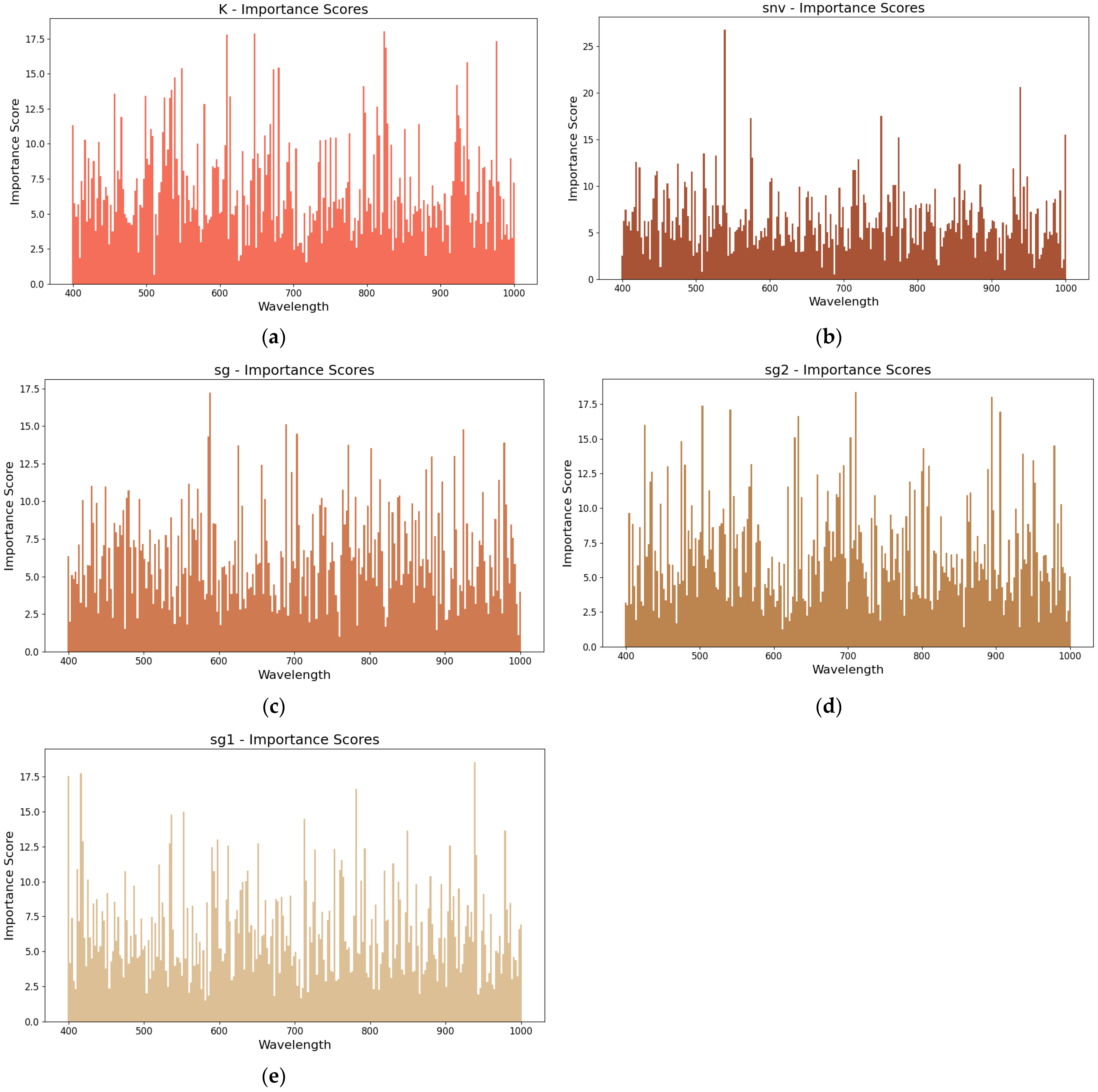
In Figure 6, the y-axis is labeled the importance score, representing the relative significance of each wavelength in the applied preprocessing methods. The figure also includes a legend to distinguish between methods like KM, SNV, SG, SG1, and SG2, providing insight into their impact on marginal contributions. The marginal contributions associated with SNV at approximately 550 nm, 750 nm, and 950 nm are considerably higher than those of other preprocessing methods at their respective wavelengths. These wavelengths are notably associated with key functional groups in SOM. The 550 nm feature corresponds to the C-H stretching overtone, while 750 nm is linked to the O-H stretching vibration. Additionally, 950 nm is associated with the O-H stretch in carboxylic acids and phenolic compounds. These functional groups, which are crucial to SOM content, contribute significantly to the spectral response and, consequently, to the inversion accuracy. The high marginal contribution at these wavelengths suggests that SNV preprocessing effectively highlights the absorption features related to these functional groups, thus enhancing SOM inversion performance in these spectral regions. Moreover, integrating multiple preprocessing strategies facilitates complementary advantages, allowing the effects of different preprocessing methods to be superimposed. For example, although SNV preprocessing enhances the useful signals for inverting SOM in general, the signal enhanced by SG2 preprocessing and SG1 preprocessing between 400 nm and 700 nm contributes more to the SOM inversion than SNV, which proves that the different wavelength bands contribute to the accuracy of the SOM inversion in a different and complementary way under different preprocessing. By applying marginal contribution analysis to uniformly evaluate the importance of each spectral band across different preprocessing methods, this study confirms the synergistic gains achievable through combined preprocessing. This reinforces the notion that multi-preprocessing approaches, which leverage the strengths of individual methods, offer superior performance compared to single preprocessing techniques. Thus, this study lays a foundation for the strategic selection and combination of preprocessing approaches, ensuring more accurate and reliable SOM inversion.
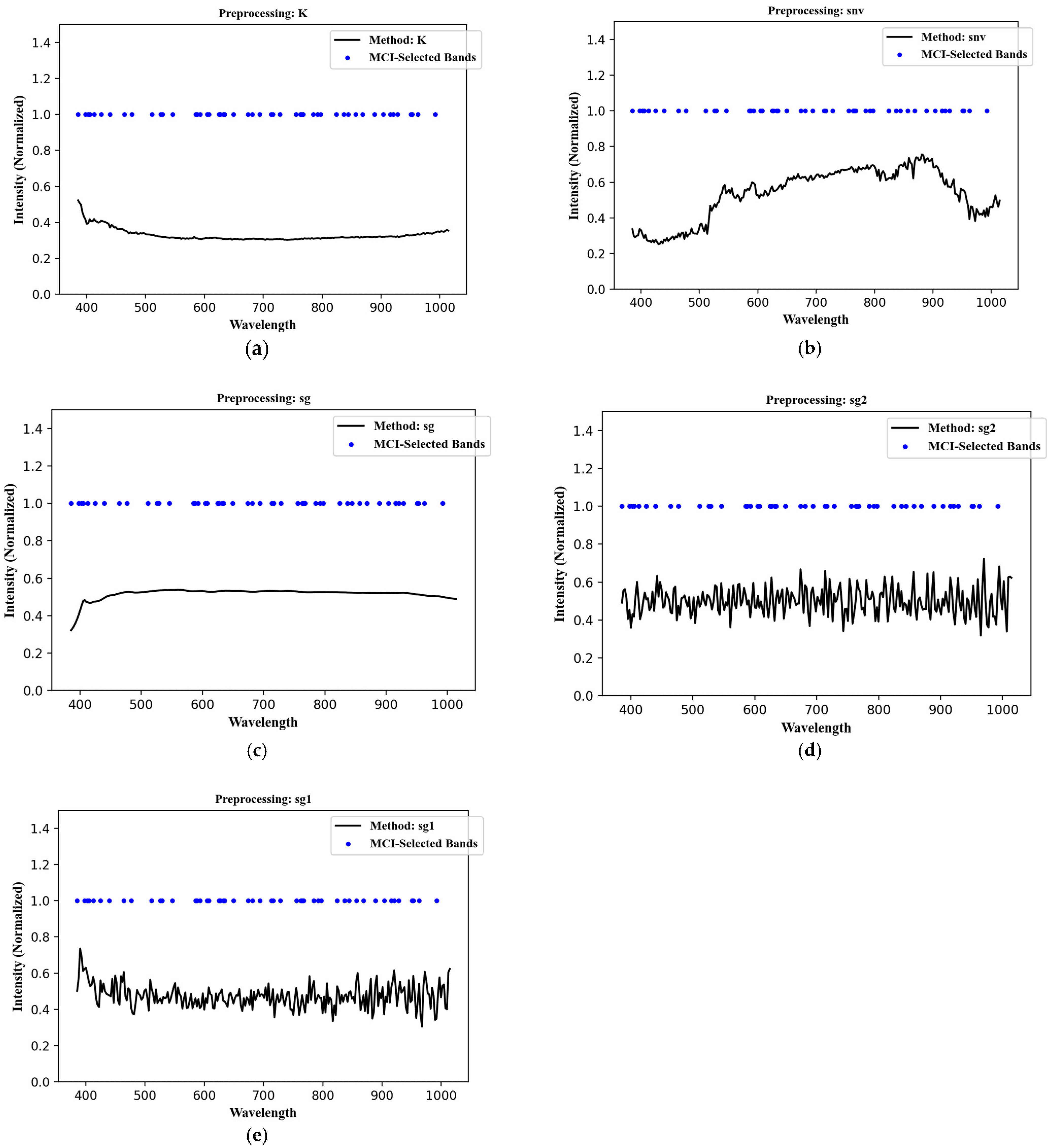
In Figure 7, the y-axis is labeled normalized intensity, indicating the intensity values of each wavelength after normalization. Figure 7 visualizes the wavelengths identified by the marginal sharing criterion as particularly influential after each preprocessing step, thereby clearly demonstrating how marginal contribution analysis guides the selection of concise yet highly informative wavelength subsets for subsequent modeling and interpretation.

3.4. Comparative Performance Analysis of MC-SFNet

A stratified five-fold cross-validation protocol was applied to the 200 black soil spectra to quantify the advantage of the proposed MC-SFNet. In each fold, 160 spectra formed the training subset and 40 spectra served as an unseen test subset. To ensure a fair benchmark, every competing approach— RF [55], PLSR [56], SVM [57], 1D-CNN [58]—and the transformer model [59] were trained and evaluated on exactly the same folds. The Transformer architecture used in this study is configured as follows: The Transformer module consists of 1 encoder layer with 4 attention heads. The convolutional part comprises 2 convolutional layers with a kernel size of 3 and a stride of 1. Positional encoding is implemented using sine–cosine encoding, and the outputs from both the CNN, which captures local features, and the Transformer, which models long-range dependencies, are fused through fully connected layers for prediction [59]. For the parameter optimization, grid search was used to find the best hyperparameters for the classical models, and band selection did not show significant improvement under single preprocessing methods in the dataset. For the SVM model, we used radial basis function as kernel function and the parameter gamma from scale [58]. For the PLSR model, we selected the optimal 10 components based on current best practices in the field [60].
MC-SFNet is trained using the Adam optimizer (learning rate = 0.0001) and MSELoss for 300 epochs with a batch size of 16, where input data is passed through the model, loss is computed, gradients are backpropagated, and model parameters are updated to minimize the loss, ensuring reproducibility of the results. Table 2 aggregates the cross-validated metrics. MC-SFNet-FIN attained an R2 of 0.80, an RMSE of 0.97 g kg−1, and a PCC of 0.90, thereby outperforming all competing methods. Due to the relatively sample size of 200 in this dataset, the range of wavelengths observed in the results is relatively broad; however, a two-tailed paired t-test confirms that the improvements achieved by MC-SFNet are statistically significant at the 1% level. While RF and SVM are computationally efficient, MC-SFNetFIN significantly outperforms them, achieving higher accuracy by capturing complex feature interactions. Its ability to enhance model precision makes it particularly valuable in applications where predictive accuracy is critical. While traditional models such as RF and SVM are highly efficient and often perform well on simpler tasks, they may not capture the intricate patterns. MC-SFNetFIN, leveraging multi-preprocessing fusion and deep learning, is designed to better capture complex feature interactions and long-range dependencies, which are especially useful when dealing with the nonlinear relationships and noise inherent in spectral data.

3.5. Generalization of Marginal Contribution-Driven Preprocessing for Enhanced Performance Across Machine Learning Models

In this section, we extend the marginal contribution-driven preprocessing framework, originally developed for the MC-SFNet, to various other machine learning models, demonstrating its generalizability and efficacy in enhancing predictive accuracy. By coupling the MC-SFNet preprocessing pipeline with classical machine learning algorithms, we observe substantial improvements in model performance, confirming the broader applicability of the marginal contribution-guided feature-level fusion strategy.
When the MC-SFNet preprocessing was combined with a RF regressor, performance metrics were significantly improved: the R2 rose to 0.75, the RMSE dropped to 1.08, and the PCC reached 0.87. Similarly, for the SVM baseline, MC-SFNet preprocessing boosted R2 to 0.75, reduced RMSE to 1.07, and increased PCC to 0.88. Even the traditional PLSR model benefited from the marginal contribution-guided preprocessing, with R2 increasing to 0.61, RMSE decreasing to 1.33, and PCC climbing to 0.79. However, the improvement for PLSR was modest—aligning with previous findings by Lin [61], who highlighted PLSR’s limitations for hyperspectral soil inversion. The overall pattern clearly shows that the MC-SFNet preprocessing approach enhances predictive accuracy across both machine learning and deep learning models.
In contrast, the proposed MC-SFNet-based framework, which integrates physical modeling with marginal-contribution analysis, consistently achieved better performance compared to traditional preprocessing methods across all tested models. These results suggest that incorporating physical constraints and marginal contribution guidance may enhance feature informativeness and model generalization, particularly for hyperspectral soil organic matter prediction.
Table 3 provides a detailed comparison of the performance of various machine learning models using different preprocessing techniques. The integration of MC-SFNet preprocessing consistently outperforms the traditional preprocessing methods across all evaluated models. Single preprocessing with the 1D-CNN serves as the baseline, while the MC-SFNet, which utilizes MCI-driven preprocessing, represents the proposed method that incorporates more advanced multi-preprocessing strategies. Single preprocessing techniques are often computationally less intensive, as they involve simpler transformations of the raw data, which can lead to faster model training times. However, these methods may not capture the complex relationships in the data as effectively as multi-preprocessing strategies. This can limit their predictive accuracy, particularly in cases involving high-dimensional data such as hyperspectral soil inversion, where more nuanced features are needed to achieve robust predictions. On the other hand, MC-SFNet’s multi-preprocessing fusion, which combines marginal contribution-driven feature selection with deep learning, significantly enhances model performance by incorporating physical modeling constraints and feature-level fusion. Although this approach demands more computational resources, especially in terms of preprocessing time and memory usage, it leads to a more informative feature set, which in turn improves the model’s ability to generalize across diverse conditions. The MCI-driven band selection approach, used in MC-SFNet, significantly reduces the computational resources required by selecting the most relevant wavelengths, yet it still provides higher inversion accuracy compared to single preprocessing methods.

3.6. Generalizability Experiments

To assess the MC-SFNet’s generalization capability, this study performed inverse measurements using MC-SFNet on different soil elements from various regions, and compared the results with those of the current algorithm. Specifically, the LUCAS dataset, which includes 19860 geo-referenced 20 cm soil samples from across the EU collected in 2009, was utilized to measure total nitrogen content. Based on the results presented in Table 4, the MC-SFNet model outperformed the other models across various performance metrics, including R2, RMSE, and PCC, demonstrating its superior ability to accurately measure total nitrogen content in the LUCAS dataset. Despite being tested on a different soil chemical element and a different geographic region, the model consistently delivered the best results, especially in comparison to traditional methods like RF, PLSR, SVM, and even advanced deep learning models such as Transformer and 1D-CNN. This highlights the robustness and generalizability of the model, further validating the proposed theory’s ability to adapt across diverse conditions and soil elements.

4. Future Work

Future research should first verify the applicability and generalizability of MC-SFNet across a broader range of soil types, geographic regions, and inversion algorithms to establish its robustness under diverse field conditions. We will also investigate the performance of MC-SFNet under complex topography, such as mountainous areas, and low SNR conditions. Strategies for mitigating topographic and shadow effects will be explored. Additionally, addressing airborne platform adaptation by accounting for sensor-specific spectral responses and atmospheric corrections will be crucial to ensure MC-SFNet’s robustness across both field and airborne applications. Embedding advanced feature integration techniques, such as self-attention mechanisms [62] and multi-head fusion strategies [63], will further enhance the quality of feature fusion and predictive performance. Continued exploration in these directions will strengthen the accuracy and robustness of soil hyperspectral inversion, providing more reliable data support for agricultural management, environmental monitoring, and related applications.

5. Conclusions

This study utilized the marginal contribution to integrate multiple soil spectral preprocessing strategies, enabling a unified analysis and interpretation of each spectral wavelength’s marginal contribution to SOM inversion performance. The findings revealed a synergistic effect among various preprocessing methods. We designed the MC-SFNet: a physics-guided, feature-level fusion architecture that couples data-driven preprocessing with the Kubelka–Munk optical model. We developed wavelength-level and feature-level fusion strategies within the MC-SFNet. The dataset consisted of imaging hyperspectral data suitable for UAV applications, comprising 200 black soil samples collected from agricultural regions in Northeastern China, rather than laboratory-based non-imaging hyperspectral data. Experimental validations demonstrated significant performance improvements, achieving a reduction in RMSE by 10.7% compared with the prevalent generalized hyperspectral soil inversion models. Furthermore, MC-SFNet surpassed established models, including PLSR, SVM, RF, 1D-CNN, and Transformer, confirming its robustness and applicability.

Author Contributions

Conceptualization, J.T.; Formal analysis, D.L.; Resources, J.L. (Junbao Li); Data curation, Q.W.; Writing – original draft, J.L. (Jingxiao Liao); Supervision, J.S. All authors have read and agreed to the published version of the manuscript.

Funding

This research received no external funding.

Data Availability Statement

Data will be made available on request.

Conflicts of Interest

The authors declare no conflict of interest.

References

  1. Trivedi, M.Y.; Patel, B.I. A study on the impact of agri-entrepreneurship in the development of the agricultural sector resulting in the upliftment of the Indian economy. Int. J. Darshan 2024, 4, 2404. [Google Scholar] [CrossRef]
  2. Sanchez, P.A.; Ahamed, S.; Carré, F.; Hartemink, A.E.; Hempel, J.; Huising, J.; Lagacherie, P.; McBratney, A.B.; McKenzie, N.J.; Mendonca-Santos, M.d.L.; et al. Digital soil map of the world. Science 2009, 325, 680–681. [Google Scholar] [CrossRef]
  3. Gerke, J. The central role of soil organic matter in soil fertility and carbon storage. Soil Syst. 2022, 6, 33. [Google Scholar] [CrossRef]
  4. Tang, J.; Wang, Q.; Liu, D. A novel approach to spectral moisture interference correction for nitrogen and soil organic matter inversion in native black soils: Bayesian-optimized dynamic moisture mitigation. Ecol. Inform. 2025, 90, 103240. [Google Scholar] [CrossRef]
  5. Stevenson, A.; Zhang, Y.K.; Huang, J.Y.; Hu, J.; Paustian, K.; Hartemink, A.E. Rates of soil organic carbon change in cultivated and afforested sandy soils. Agric. Ecosyst. Environ. 2024, 360, 108785. [Google Scholar] [CrossRef]
  6. Ma, Y.Q.; Woolf, D.; Fan, M.S.; Qiao, L.; Li, R.; Lehmann, J. Global crop production increase by soil organic carbon. Nat. Geosci. 2023, 16, 1159–1165. [Google Scholar] [CrossRef]
  7. Lal, R. Soil carbon sequestration impacts on global climate change and food security. Science 2004, 304, 1623–1627. [Google Scholar] [CrossRef] [PubMed]
  8. Futa, B.; Gmitrowicz-Iwan, J.; Skersienė, A.; Šlepetienė, A.; Parašotas, I. Innovative soil management strategies for sustainable agriculture. Sustainability 2024, 16, 9481. [Google Scholar] [CrossRef]
  9. Shen, L.; Gao, M.; Yan, J.; Li, Z.-L.; Leng, P.; Yang, Q.; Duan, S.-B. Hyperspectral estimation of soil organic matter content using different spectral pre-processing techniques and PLSR method. Remote Sens. 2020, 12, 1206. [Google Scholar] [CrossRef]
  10. Francos, N.; Nasta, P.; Allocca, C.; Sica, B.; Mazzitelli, C.; Lazzaro, U.; D’urso, G.; Belfiore, O.R.; Crimaldi, M.; Sarghini, F.; et al. Mapping soil organic carbon stock using hyperspectral remote sensing: A case study in the Sele River Plain in Southern Italy. Remote Sens. 2024, 16, 897. [Google Scholar] [CrossRef]
  11. Yan, Y.; Yang, J.; Li, B.; Qin, C.; Ji, W.; Xu, Y.; Huang, Y. High-resolution mapping of soil organic matter at the field scale using UAV hyperspectral images with a small calibration dataset. Remote Sens. 2023, 15, 1433. [Google Scholar] [CrossRef]
  12. Bouslihim, Y.; Bouasria, A.; Minasny, B.; Castaldi, F.; Nenkam, A.M.; El Battay, A.; Chehbouni, A. Soil organic carbon prediction and mapping in Morocco using PRISMA hyperspectral imagery and meta-learner model. Remote Sens. 2025, 17, 1363. [Google Scholar] [CrossRef]
  13. Bouslihim, Y.; Bouasria, A. Potential of EnMAP hyperspectral imagery for regional-scale soil organic matter mapping. Remote Sens. 2025, 17, 1600. [Google Scholar] [CrossRef]
  14. Meng, X.; Bao, Y.; Ye, Q.; Liu, H.; Zhang, X.; Tang, H.; Zhang, X. Soil organic matter prediction model with satellite hyperspectral image based on optimized denoising method. Remote Sens. 2021, 13, 2273. [Google Scholar] [CrossRef]
  15. Cezar, E.; Alberton, T.A.; Lemos, E.F.; de Oliveira, K.M.; Sun, L.; Crusiol, L.G.T.; Rodrigues, M.; Reis, A.S.; Nanni, M.R. Estimating soil organic matter using proximal remote sensing: Performance evaluation of prediction models adjusted at local scale in the Brazilian Cerrado. Remote Sens. 2023, 15, 4397. [Google Scholar] [CrossRef]
  16. Rasooli, N.; Mirzaei, S.; Pignatti, S. Monitoring gypsiferous soils by leveraging advanced spaceborne hyperspectral imagery via spectral indices and a machine learning approach. Remote Sens. 2025, 17, 1914. [Google Scholar] [CrossRef]
  17. Lima, A.A.J.; Lopes, J.C.; Lopes, R.P.; de Figueiredo, T.; Vidal-Vázquez, E.; Hernández, Z. Soil organic carbon assessment using remote-sensing data and machine learning: A systematic literature review. Remote Sens. 2025, 17, 882. [Google Scholar] [CrossRef]
  18. Li, T.; Cui, L.; Wu, Y.; McLaren, T.I.; Xia, A.; Pandey, R.; Liu, H.; Wang, W.; Xu, Z.; Song, X.; et al. Soil organic carbon estimation via remote sensing and machine learning techniques: Global topic modeling and research trend exploration. Remote Sens. 2024, 16, 3168. [Google Scholar] [CrossRef]
  19. Nelson, D.W.; Sommers, L.E. Total carbon, organic carbon, and organic matter. In Methods of Soil Analysis, Part 3: Chemical Methods; Sparks, D.L., Ed.; Soil Science Society of America: Madison, WI, USA, 1996; pp. 961–1010. [Google Scholar] [CrossRef]
  20. Aj, S.; Adhikari, K.; Dharumarajan, S.; Lalitha, M. Remote sensing and geographic information system applications in mapping and assessment of soil resources. In Remote Sensing of Soils; Elsevier: Amsterdam, The Netherlands, 2024. [Google Scholar] [CrossRef]
  21. Vavlas, N.-C.; Porre, R.; Meng, L.; Elhakeem, A.; van Egmond, F.; Kooistra, L.; De Deyn, G.B. Cover crop impacts on soil organic matter dynamics and its quantification using UAV and proximal sensing. Smart Agric. Technol. 2024, 9, 100621. [Google Scholar] [CrossRef]
  22. Viscarra Rossel, R.A.; Webster, R. Predicting soil properties from the Australian soil visible–near infrared spectroscopic database. Eur. J. Soil Sci. 2012, 63, 848–860. [Google Scholar] [CrossRef]
  23. Shi, T.; Cui, L.; Wang, J.; Fei, T.; Chen, Y.; Wu, G. Comparison of multivariate methods for estimating soil total nitrogen with visible/near-infrared spectroscopy. Plant Soil 2013, 366, 363–375. [Google Scholar] [CrossRef]
  24. Feng, Y.; Wang, J.L.; Tang, Y.L. Estimation and inversion of soil heavy metal arsenic (As) based on UAV hyperspectral platform. Microchem. J. 2024, 207, 112027. [Google Scholar] [CrossRef]
  25. Sun, M.; Yang, Y.; Li, S.; Yin, D.; Zhong, G.; Cao, L. A study on hyperspectral soil total nitrogen inversion using a hybrid deep learning model CBiResNet-BiLSTM. Chem. Biol. Eng. Q. 2024, 11, 157. [Google Scholar] [CrossRef]
  26. Zhong, Q.; Eziz, M.; Ainiwaer, M.; Sawut, R.; Hou, M. Hyperspectral estimation of mercury content of soil in oasis city in arid zones of China. Geocarto Int. 2024, 39, 2299147. [Google Scholar] [CrossRef]
  27. Subi, X.; Eziz, M.; Zhong, Q.; Li, X.G. Estimating the chromium concentration of farmland soils in an arid zone from hyperspectral reflectance by using partial least squares regression methods. Ecol. Indic. 2024, 161, 111987. [Google Scholar] [CrossRef]
  28. Zhao, W.; Wu, Z.; Yin, Z.; Li, D. Attention-based CNN ensemble for soil organic carbon content estimation with spectral data. IEEE Geosci. Remote Sens. Lett. 2022, 19, 6013105. [Google Scholar] [CrossRef]
  29. Kawamura, K.; Nishigaki, T.; Andriamananjara, A.; Rakotonindrina, H.; Tsujimoto, Y.; Moritsuka, N.; Rabenarivo, M.; Razafimbelo, T. Using a one-dimensional convolutional neural network on visible and near-infrared spectroscopy to improve soil phosphorus prediction in Madagascar. Remote Sens. 2021, 13, 1519. [Google Scholar] [CrossRef]
  30. Wang, Z.; Zhang, Q.; Li, J. Soil moisture prediction using deep learning methods and hyperspectral data. Environ. Sci. Technol. 2023, 57, 789–801. [Google Scholar] [CrossRef]
  31. Li, X.; Zhang, L.; Wei, Y. Soil texture classification based on hyperspectral data and convolutional neural networks. J. Soil Sci. Environ. Manage. 2023, 45, 1123–1134. [Google Scholar] [CrossRef]
  32. Cao, Y.; Yang, W.; Li, H.; Zhang, H.; Li, M.Z. Development of a vehicle-mounted soil organic matter detection system based on near-infrared spectroscopy and image information fusion. Measurement Sci. Technol. 2024, 35, 045501. [Google Scholar] [CrossRef]
  33. Patel, A.K.; Ghosh, J.K.; Pande, S.; Sayyad, S.U. Deep-learning-based approach for estimation of fractional abundance of nitrogen in soil from hyperspectral data. IEEE J. Sel. Top. Appl. Earth Obs. Remote Sens. 2020, 13, 6495. [Google Scholar] [CrossRef]
  34. Barra, I.; Haefele, S.M.; Sakrabani, R.; Kebede, F. Soil spectroscopy with the use of chemometrics, machine learning and pre-processing techniques in soil diagnosis: Recent advances—A review. Trends Anal. Chem. 2021, 135, 116166. [Google Scholar] [CrossRef]
  35. Zhang, M.; Li, M.; Liu, W.; Cui, L.; Li, W.; Wang, H.; Wei, Y.; Guo, Z.; Wang, D.; Hu, Y.; et al. Analyzing the performance of statistical models for estimating leaf nitrogen concentration of Phragmites australis based on leaf spectral reflectance. Spectrosc. Lett. 2019, 52, 483–491. [Google Scholar] [CrossRef]
  36. He, J.; Liu, G.; Li, W.; Li, Z.; Li, Z. Inversion analysis of soil nitrogen content using hyperspectral images with different pre-processing methods. Ecol. Inform. 2023, 78, 102381. [Google Scholar] [CrossRef]
  37. Xu, X.B.; Ma, F.; Zhou, J.M.; Du, C.W. Applying convolutional neural networks (CNN) for end-to-end soil analysis based on laser-induced breakdown spectroscopy (LIBS) with less spectral pre-processing. Comput. Electron. Agric. 2022, 199, 107171. [Google Scholar] [CrossRef]
  38. Catav, A.; Fu, B.; Zoabi, Y.; Weiss-Meilik, A.; Shomron, N.; Ernst, J.; Sankararaman, S.; Gilad-Bachrach, R. Marginal contribution feature importance—An axiomatic approach for explaining data. Proc. Mach. Learn. Res. 2021, 139, 1324–1335. [Google Scholar] [CrossRef]
  39. Ye, S.; Weng, H.; Xiang, L.; Jia, L.; Xu, J. Synchronously predicting tea polyphenol and epigallocatechin gallate in tea leaves using Fourier transform–near-infrared spectroscopy and machine learning. Molecules 2023, 28, 5379. [Google Scholar] [CrossRef] [PubMed]
  40. Wang, B.; Yang, H.; Zhang, S.; Li, L. Detection of defective features in Cerasus Humilis fruit based on hyperspectral imaging technology. Appl. Sci. 2023, 13, 3279. [Google Scholar] [CrossRef]
  41. Liu, X.; Tang, X.; Guo, J.; Lin, L.; Huang, F.; Robert, E. Concentration prediction of imidacloprid in water through the combination of Fourier transform infrared spectral data and 1D CNN with multilevel feature fusion. Desalination Water Treat. 2022, 274, 130–139. [Google Scholar] [CrossRef]
  42. Ou, D.; Tan, K.; Li, J.; Wu, Z.; Zhao, L.; Ding, J.; Wang, X.; Zou, B. Prediction of soil organic matter by Kubelka–Munk based airborne hyperspectral moisture removal model. Int. J. Appl. Earth Obs. Geoinf. 2023, 124, 103493. [Google Scholar] [CrossRef]
  43. Wang, Y.; Li, M.; Ji, R.; Wang, M.; Zheng, L. A deep learning-based method for screening soil total nitrogen characteristic wavelengths. Comput. Electron. Agric. 2021, 187, 106228. [Google Scholar] [CrossRef]
  44. Ma, X.; Wang, J.; Zhou, K.; Zhang, W.; Zhang, Z.; Zhou, S.; Bai, Y.; De Maeyer, P.; Van de Voorde, T. Quantitative evaluation of the impact of band optimization methods on the accuracy of the hyperspectral metal element inversion models. Int. J. Appl. Earth Obs. Geoinf. 2024, 132, 104011. [Google Scholar] [CrossRef]
  45. Zhang, X.; Wen, J.T.; Zhao, D. Band selection method for retrieving soil lead content with hyperspectral remote sensing data. In Earth Resources and Environmental Remote Sensing-GIS Applications; Michel, U., Civco, D.L., Eds.; Proceedings of SPIE 2010; SPIE: Bellingham, WA, USA, 2010; Volume 7831, p. 78311K. [Google Scholar] [CrossRef]
  46. Zhang, J.; Cui, X.Y.; Cai, W.S.; Shao, X.G. Combination of heuristic optimal partner wavelengths for variable selection in near-infrared spectral analysis. J. Chemom. 2018, 32, e2971. [Google Scholar] [CrossRef]
  47. Chander Goud, S.; Subhash, O.; Goud, C.; Sarma, T.H.; Bindu, C.S. Optimal wavelength selection in hyperspectral images using improved K-means clustering with spectral similarity measures. In Proceedings of the 2023 IEEE International Conference on Artificial Intelligence in Engineering and Technology (IICAIET), Kota Kinabalu, Malaysia, 12–14 September 2023. [Google Scholar] [CrossRef]
  48. Zhao, Y.; Li, X.L. Deep spectral clustering with regularized linear embedding for hyperspectral image clustering. IEEE Trans. Geosci. Remote Sens. 2023, 61, 5509311. [Google Scholar] [CrossRef]
  49. Liu, B.Y.; Guo, B.F.; Zhuo, R.X.; Dai, F. Estimation of soil organic carbon content by Vis-NIR spectroscopy combining feature selection algorithm and local regression method. Rev. Bras. Cienc. Solo 2023, 47, e0230067. [Google Scholar] [CrossRef]
  50. Lundberg, S.M.; Lee, S.-I. A unified approach to interpreting model predictions. In Advances in Neural Information Processing Systems; 2017; pp. 4765–4774. Available online: https://dl.acm.org/doi/10.5555/3295222.3295230 (accessed on 8 August 2025).
  51. Zhong, L.; Guo, X.; Ding, M.; Ye, Y.; Zhu, Q.; Guo, J.; Wu, J.; Zeng, X. Spatial mapping of topsoil total nitrogen in mountainous and hilly areas of southern China using a continuous convolution neural network. Catena 2023, 229, 107228. [Google Scholar] [CrossRef]
  52. Misbah, K.; Laamrani, A.; Voroney, P.; Khechba, K.; Casa, R.; Chehbouni, A. Ensemble band selection for quantification of soil total nitrogen levels from hyperspectral imagery. Remote Sens. 2024, 16, 2549. [Google Scholar] [CrossRef]
  53. Pan, S.; Liu, Z.; Han, Y.; Zhang, D.; Zhao, X.; Li, J.; Wang, K. Using the Pearson’s correlation coefficient as the sole metric to measure the accuracy of quantitative trait prediction: Is it sufficient? Front. Plant Sci. 2024, 15, 1480463. [Google Scholar] [CrossRef]
  54. Gao, Z.L.; Wang, W.Q.; Wang, H.J.; Li, R.Y. Selection of spectral parameters and optimization of estimation models for soil total nitrogen content during fertilization period in apple orchards. Horticulturae 2024, 10, 358. [Google Scholar] [CrossRef]
  55. Ma, Y.; Jiang, Q.G.; Meng, Z.G.; Liu, H.X. Black soil organic matter content estimation using hybrid selection method based on RF and GABPSO. Spectrosc. Spect. Anal. 2018, 38, 181–187. [Google Scholar]
  56. Hati, K.M.; Sinha, N.; Mohanty, M.; Jha, P.; Londhe, S.; Sila, A.; Towett, E.; Chaudhary, R.; Jayaraman, S.; Vassanda Coumar, M.; et al. Mid-infrared reflectance spectroscopy for estimation of soil properties of Alfisols from Eastern India. Sustainability 2022, 14, 94883. [Google Scholar] [CrossRef]
  57. Shen, Z.; Viscarra Rossel, R.A. Automated spectroscopic modelling with optimised convolutional neural networks. Sci. Rep. 2021, 11, 208. [Google Scholar] [CrossRef] [PubMed]
  58. Zhong, L.; Guo, X.; Ding, M.; Ye, Y.; Jiang, Y.; Zhu, Q.; Li, J. SHAP values accurately explain the difference in modeling accuracy of convolution neural network between soil full-spectrum and feature-spectrum. Comput. Electron. Agric. 2024, 217, 108627. [Google Scholar] [CrossRef]
  59. Cao, L.; Sun, M.; Yang, Z.; Jiang, D.; Yin, D.; Duan, Y. A Novel Transformer-CNN Approach for Predicting Soil Properties from LUCAS Vis-NIR Spectral Data. Agronomy 2024, 14, 1998. [Google Scholar] [CrossRef]
  60. Canero, F.M.; Rodriguez-Galiano, V.; Aragones, D. Machine Learning and Feature Selection for Soil Spectroscopy: An Evaluation of Random Forest Wrappers to Predict Soil Organic Matter, Clay, and Carbonates. Heliyon 2024, 10, e30228. [Google Scholar] [CrossRef]
  61. Lin, L.; Gao, Z.; Liu, X. Estimation of soil total nitrogen using the synthetic color learning machine (SCLM) method and hyperspectral data. Geoderma 2020, 380, 114664. [Google Scholar] [CrossRef]
  62. Vaswani, A.; Shazeer, N.; Parmar, N.; Uszkoreit, J.; Jones, L.; Gomez, A.N.; Kaiser, Ł.; Polosukhin, I. Attention is all you need. Adv. Neural Inf. Process. Syst. 2017, 30, 5998–6008. [Google Scholar] [CrossRef]
  63. Niu, Z.; Zhong, G.; Yu, H. A review on the attention mechanism of deep learning. Neurocomputing 2021, 452, 48–62. [Google Scholar] [CrossRef]
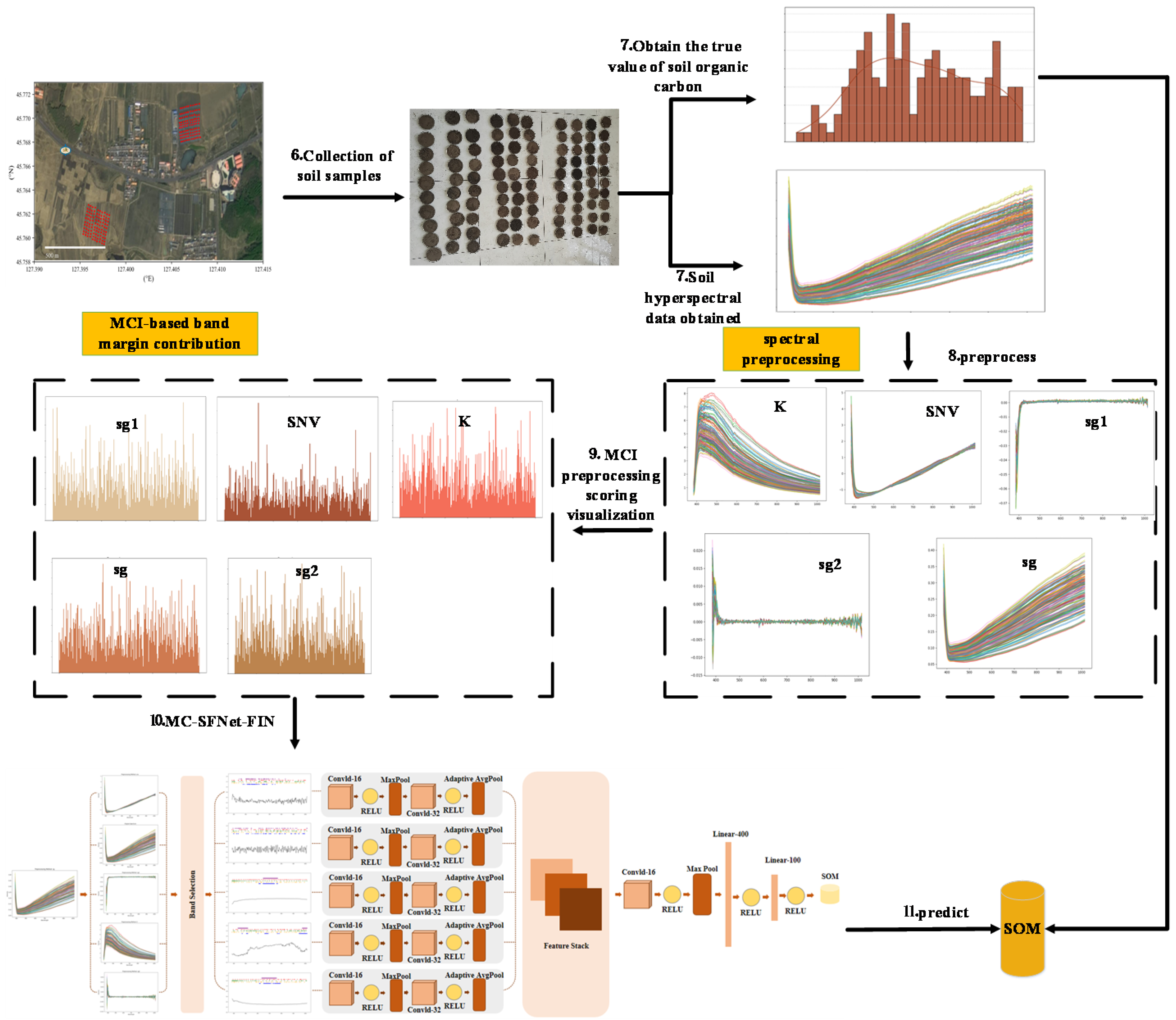
Figure 1. Workflow of the data analysis methodology applied in this study.
Remotesensing 17 02806 g001
Figure 2. Visualization of different preprocessing methods: (a) KM preprocessing, (b) SNV preprocessing, (c) SG1 preprocessing, (d) SG2 preprocessing, (e) SG preprocessing.
Remotesensing 17 02806 g002
Figure 3. Marginal contribution-driven spectral fusion network: (a) wavelength-level spectral fusion; (b) feature-level spectral fusion.
Remotesensing 17 02806 g003
Figure 4. Soil sample collection sites.
Remotesensing 17 02806 g004
Figure 5. Distribution of soil samples.
Remotesensing 17 02806 g005
Figure 6. Marginal contributions of wavelengths: (a) importance of KM wavelength, (b) importance of SNV wavelength, (c) importance of SG wavelength, (d) importance of SG2 wavelength, (e) importance of SG1 wavelength.
Remotesensing 17 02806 g006
Figure 7. Visualization of wavelength selection: (a) wavelength selection for KM, (b) wavelength selection for snv, (c) wavelength selection for sg, (d) wavelength selection for sg2, (e) wavelength selection for sg1.
Remotesensing 17 02806 g007
Table 1. MC-SFNet network architecture.
Layer TypeOutput Shape
Input(batch_size, preprocess, features)
Conv1d(batch_size, 16, features)
Max Pooling (batch_size, 16, features/2)
Conv1d (batch_size, 32, features/2)
Max Pooling (batch_size, 32, features/4)
Adaptive Pooling(batch_size, 32, 128)
Global Conv1d(batch_size, 32, global_output)
Linear Layer 1(batch_size, 400)
ReLU(batch_size, 400)
Linear Layer 2(batch_size, 100)
ReLU (batch_size, 100)
Output(batch_size, 1)
Table 2. Comparison of the inversion accuracy of MC-SFNet.
Model
RF [55]plsr [56]svm [57]1D-CNN [58]Transformer [59]MC-SFNet-WINMC-SFNetFIN
R20.73 ± 0.090.59 ± 0.080.72 ± 0.100.71 ± 0.150.75 ± 0.140.78 ± 0.090.80 ± 0.08
RMSE1.11 ± 0.191.37 ± 0.071.13 ± 0.171.15 ± 0.271.07 ± 0.261.00 ± 0.160.97 ± 0.15
PCC0.86 ± 0.050.78 ± 0.050.86 ± 0.060.85 ± 0.050.89 ± 0.060.90 ± 0.050.90 ± 0.05
Table 3. Performance comparison of different preprocessing techniques for various machine learning models.
Preprocessing
SG [39]SG1 [40]SG2SNV [41]MCI-Driven
RF [55]R20.410.500.170.710.75
RMSE1.661.521.951.151.08
PCC0.660.730.420.850.87
plsr [56]R20.560.23−0.270.480.61
RMSE1.411.872.411.531.33
PCC0.770.630.430.740.79
svm [57]R20.290.710.150.730.75
RMSE1.811.161.991.121.07
PCC0.560.850.410.860.88
1D-CNN [58]R20.270.590.160.710.78
RMSE1.831.381.961.171.00
PCC0.550.780.450.840.89
Table 4. Inverse measurement of total nitrogen content on the LUCAS dataset.
Model
RF [55]plsr [56]svm [57]1D-CNN [58]Transformer [59]MC-SFNet-WINMC-SFNetFIN
R20.890.850.810.890.930.940.95
RMSE1.211.401.571.190.970.450.41
PCC0.940.920.900.950.960.970.97
Disclaimer/Publisher’s Note: The statements, opinions and data contained in all publications are solely those of the individual author(s) and contributor(s) and not of MDPI and/or the editor(s). MDPI and/or the editor(s) disclaim responsibility for any injury to people or property resulting from any ideas, methods, instructions or products referred to in the content.