Article

A Linear Feature-Based Method for Signal Photon Extraction and Bathymetric Retrieval Using ICESat-2 Data

1
Key Laboratory of Technology in Geo-Spatial Information Processing and Application System, Aerospace Information Research Institute, Chinese Academy of Sciences, Beijing 100190, China
2
Key Laboratory of Target Cognition and Application Technology, Aerospace Information Research Institute, Chinese Academy of Sciences, Beijing 100190, China
3
School of Electronic, Electrical and Communication Engineering, University of Chinese Academy of Sciences, Beijing 100049, China
4
Geological Exploration Institute of Shandong Zhengyuan, China Metallurgical Geology Bureau, Jinan 250101, China
5
National Institute of Natural Hazards, Ministry of Emergency Management of China, Beijing 100085, China
*
Author to whom correspondence should be addressed.
Remote Sens. 2025, 17(16), 2792; https://doi.org/10.3390/rs17162792
Submission received: 18 May 2025 / Revised: 13 July 2025 / Accepted: 6 August 2025 / Published: 12 August 2025
(This article belongs to the Section Earth Observation Data)

Abstract

The ATL03 data from the photon-counting LiDAR onboard the Ice, Cloud, and Land Elevation Satellite-2 (ICESat-2) holds substantial potential for shallow-water bathymetry due to its high sensitivity and broad spatial coverage. However, distinguishing signal photons from noise in low-photon-density and complex terrain environments remains a significant challenge. This study proposes an adaptive photon extraction algorithm based on linear feature analysis, incorporating resolution adjustment, segmented Gaussian fitting, and linear feature-based signal identification. To address the reduction in signal photon density with increasing water depth, the method employs a depth-dependent adaptive neighborhood search radius, which dynamically expands into deeper regions to ensure reliable local feature computation. Experiments using eight ICESat-2 datasets demonstrated that the proposed method achieves average precision and recall values of 0.977 and 0.958, respectively, with an F1 score of 0.967 and an overall accuracy of 0.972. The extracted bathymetric depths demonstrated strong agreement with the reference Continuously Updated Digital Elevation Model (CUDEM), achieving a coefficient of determination of 0.988 and a root mean square error of 0.829 m. Compared to conventional methods, the proposed approach significantly improves signal photon extraction accuracy, adaptability, and parameter stability, particularly in sparse photon and complex terrain scenarios. In comparison with the DBSCAN algorithm, the proposed method achieves a 30.0% increase in precision, 17.3% improvement in recall, 24.3% increase in F1 score, and 22.2% improvement in overall accuracy. These findings confirm the effectiveness and robustness of the proposed algorithm for ICESat-2 shallow-water bathymetry applications.

1. Introduction

Marine surveying serves as the foundation for marine economic development and environmental protection, with one of its fundamental tasks being the measurement of seafloor depths around islands, reefs, and their surrounding areas [1,2]. Traditional bathymetric methods primarily rely on shipborne sonar and airborne LiDAR systems [3], which are often limited by operational costs, restricted coverage in shallow or reef-dense areas, and challenges in remote or open-ocean environments [4,5,6].
At present, photon-counting LiDAR has been increasingly applied in shallow-water bathymetry due to its broad spatial coverage across remote and coastal regions and high measurement accuracy [7,8]. The Advanced Topographic Laser Altimeter System (ATLAS) instrument onboard the Ice, Cloud, and Land Elevation Satellite-2 (ICESat-2) is a photon-counting LiDAR system capable of emitting laser pulses at a high frequency of 10 kHz and capturing returning photons to generate high-density photon data [9]. The ICESat-2 laser altimetry system emits laser beams with a wavelength of 532 nm, which are reflected by the water surface and received by the system to obtain water surface elevation. Due to the weak absorption of this wavelength by water, a portion of the laser penetrates the water surface, reflects off the seafloor, and returns, enabling the retrieval of seafloor elevation and the calculation of water depth. This provides a novel approach to shallow-water bathymetry.
Compared to traditional shallow-water bathymetry methods, the ICESat-2 satellite offers advantages in acquiring shallow-water depth data with periodicity, low cost, and high accuracy [10]. Existing studies indicate that ICESat-2 demonstrates high accuracy and capability in bathymetric mapping [11]. Gleason et al. [12] compared ICESat-2-derived bathymetry with single-beam echo sounder measurements collected in the field, revealing a high correlation (R2 = 0.96). Coveney et al. [13] evaluated the vertical accuracy of ICESat-2 coastal ocean bathymetric data at four test sites in mid-latitude temperate regions, reporting an error of 0.54 m at a maximum photon depth of 11 m.
ICESat-2 utilizes photon-counting technology to detect returning photons. This technology is highly sensitive, capable of capturing extremely weak signals. However, its high sensitivity also makes it highly susceptible to various sources of background noise, including solar background light, cloud reflections, and atmospheric scattering [14,15]. This issue is particularly pronounced in daytime data, where sunlight at the 532 nm wavelength is reflected onto the ATLAS instrument, leading to significantly more noise photons in daytime data compared to nighttime data [10]. To extract accurate terrain and bathymetric information from photon data, it is necessary to design and apply noise recognition algorithms capable of distinguishing and removing noise photons effectively.
Based on the distribution characteristics of signal photons and noise photons in ICESat-2 data, existing denoising algorithms mainly focus on using density thresholds to distinguish between signal photons and noise photons [16,17]. The core idea of density threshold clustering algorithms is to perform clustering by analyzing the local density classifications of sample data. Common density clustering algorithms include Density-Based Spatial Clustering of Applications with Noise (DBSCAN) and Ordering Points To Identify the Clustering Structure (OPTICS) [16,18,19]. Determining the search radius and the number of neighboring points becomes crucial in density-based denoising algorithms. Regarding the search radius, researchers have developed denoising neighborhoods of different shapes—such as circular, elliptical, and rectangular—and determined their sizes based on terrain characteristics [10,18]. As for the number of neighboring points, the main method currently is to manually specify this number based on experience.
For seafloor photons, laser pulses penetrate the water surface to reach the seafloor but are affected by water column scattering and reflection during transmission. This causes the spatial characteristics and density distribution of photons to differ significantly from other surface types [7]. To address the attenuation of seafloor photon data with depth, some researchers have designed algorithms that segment along the elevation direction and adaptively determine the photon count threshold for each segment [20]. Chen, Le, Zhang, Wang, Qiu, and Wang [9] improved the standard DBSCAN algorithm and proposed the Adaptive Variable Ellipse-Based Method (AVEBM). AVEBM uses an elliptical filter to replace the circular filter in the standard DBSCAN algorithm and employs elliptical windows of varying sizes and orientations to search for signal photons within the neighborhood, achieving better filtering results. Wang et al. [21] further improved the OPTICS algorithm by combining adaptive variable ellipses and B-spline curve iterative filtering to detect seafloor signal photons, resulting in higher F1 scores compared to the AVEBM.
The above methods are mainly based on clustering algorithms and belong to unsupervised learning. Since the categories of classification are unknown in advance, clusters are formed by directly measuring the similarities between data points. With the development of machine learning technology, some researchers have adopted machine learning techniques to automatically distinguish between seafloor signal photons and noise [22]. Currently, common machine learning algorithms such as decision trees, K-Nearest Neighbors algorithms, and neural networks have been applied in seafloor topography photon recognition [11]. Lin and Jensen Knudby [23] proposed a method using the deep learning model PointNet++ to automatically extract seafloor bathymetric photons from ICESat-2 satellite data, involving steps like data preprocessing and labeling, model training, and model validation and testing. Machine learning methods require predefined classification attributes and labels; through learning, a classification model is obtained to categorize new data into our predefined classes [24]. As a data-driven approach, the performance of machine learning heavily depends on the quality and quantity of data. The accuracy, coverage, and quantity of labeled sample data directly affect the model’s classification effectiveness [25]. Manually creating a large number of labeled training sets is not only expensive and time-consuming but also challenging to obtain sufficiently accurate labels for many tasks. Additionally, this process places higher demands on computer hardware [26]. In view of this, this paper continues to focus on designing parameter-based algorithms to identify signal photons.
This study presents a Linear Feature-Based Signal Photon Extraction (LFSPE) method to improve the accuracy and robustness of signal photon identification for bathymetric retrieval. The LFSPE algorithm exploits the spatial distribution characteristics of photon data through a structured three-stage approach: preprocessing, coarse segmentation, and fine extraction.
In shallow-water ICESat-2 ATL03 data, bottom-return signal photons typically exhibit spatial continuity and align along approximately linear or gently curved paths that follow the laser track. This spatial structure arises from the physical properties of the seafloor and the temporal–spatial coherence of photon returns from smooth underwater surfaces. In contrast, noise photons from atmospheric scattering or background illumination appear more randomly distributed and lack such spatial regularity. Leveraging this intrinsic difference, the LFSPE method employs local linear feature analysis to effectively distinguish signal photons from noise photons.
In the preprocessing stage, the vertical and horizontal resolutions of raw ICESat-2 data are adjusted to enhance the spatial organization of signal photons and ensure uniform data quality. In the coarse segmentation stage, a segmented Gaussian fitting-based coarse segmentation is performed to distinguish underwater photons from non-underwater ones, effectively separating sea surface returns from seafloor signals. Compared with traditional density-based clustering methods such as DBSCAN, LFSPE introduces a dynamic extraction strategy based on local linear feature analysis, incorporating point density and goodness-of-fit metrics. This approach addresses the limitations of fixed-parameter clustering by enhancing adaptability to varying photon densities and complex terrain conditions. In the final fine extraction stage, LFSPE identifies signal photons that exhibit continuity and alignment along locally linear structures, using a variable neighborhood search radius that expands with depth to compensate for signal sparsity. This enables accurate and robust seafloor photon identification for shallow-water bathymetry.

2. Materials and Methods

2.1. Study Area

To evaluate the performance of the proposed method, eight diverse research areas worldwide were selected, featuring varying terrains, landforms, and maximum water depths, as shown in Figure 1. These areas include the west coast of Oahu, Hawaii (1), characterized by dry tropical conditions and coastal plains backed by the Ko’olau mountain range; Long Cay in the Bahamas (2), a narrow tropical marine island with diverse landscapes such as coral reefs and limestone hills; Playa La Chiva on Vieques Island, Puerto Rico (3), known for its sandy beaches and tropical marine climate; and Playa Blanca in northeastern Vieques Island (4), a crescent-shaped beach with lush tropical vegetation. Other areas include the reef northeast of Songo Songo Island, Tanzania (5), surrounded by coral ecosystems; the Bir Ali-Balhaf Marine Reserve in Yemen (6), featuring sandy beaches, mangroves, and coral reefs; Socotra Island in the Arabian Sea (7), with diverse coastal and inland terrains; and Coral Island in Yongle Atoll, Xisha Islands, China (8), an elliptical island encircled by lagoons and coral reefs. These sites represent a range of coastal and reef environments with unique geographic and climatic features.

2.2. Data

2.2.1. ATLAS Datasets

ICESat-2 is the successor satellite to ICESat, launched by NASA in September 2018 to continue the ICESat mission. ATLAS is the core payload of ICESat-2, designed to emit and receive laser signals for precise measurement of Earth’s surface elevation. ATLAS uses a photon-counting LiDAR system with a 532 nm wavelength to emit six laser beams arranged in three pairs, with a beam spacing of 3.3 km and a pair spacing of 90 m. The laser pulse repetition rate is up to 10 kHz. ATL03 data is one of the core products of ICESat-2, recording the acquisition time, longitude, latitude, elevation, and confidence level associated with each photon event. An ATL03 file contains data from six laser beams: gt1l, gt1r, gt2l, gt2r, gt3l, and gt3r. Given the location of the validation data and the quality of the ICESat-2 data in the study areas, detailed information about the eight selected experimental datasets, corresponding to the eight study areas labeled (1)–(8) in Figure 1, is shown in Table 1. The density in Table 1 refers to the average photon density, i.e., the number of photons per unit along the track distance, which reflects the sparsity or density of the photon data in the study areas. The ATL03 data were downloaded fromNASA’s Earthdata Search platform: https://search.earthdata.nasa.gov (accessed on 5 August 2025).
The photon distribution characteristics and photon density variations differ across the datasets. Datasets 1, 3, 4, and 6 were observed during the day, with more noise photons, making it difficult to distinguish signal photons from the noise, particularly in dataset 1, which has the greatest depth. Datasets 2, 5, 7, and 8 were observed at night, with clearer signal photon characteristics. Dataset 7 has a lower photon density, making it a sparse dataset, while dataset 8 has a higher photon density. The varying sparsity, depth, and noise levels of these datasets pose higher demands on the robustness of the extraction algorithm.

2.2.2. CUDEM Bathymetric Data

The Continuously Updated Digital Elevation Model (CUDEM) is a high-resolution land–sea integrated digital elevation model dataset developed by the National Oceanic and Atmospheric Administration (NOAA) [27]. The model integrates elevation data from various sources, including LiDAR, sonar, and satellite-derived data, providing seamless coverage for coastal and nearshore regions. CUDEM has a resolution of 1/9 arc-second (approximately 3 m), offering fine and accurate elevation measurements, making it particularly suitable for hydrodynamic modeling, coastline analysis, and bathymetric studies. According to NOAA documentation, the vertical accuracy of CUDEM is approximately 50 cm, and the horizontal accuracy is approximately 100 cm. The dataset is regularly updated to ensure it contains the most current observational data and corrections. With its high spatial resolution and comprehensive coverage of coastal topography and water depths, CUDEM is used in this study as a reference to validate ICESat-2 bathymetric data. Due to differences in geodetic and elevation baselines between CUDEM and ICESat-2, a baseline conversion tool provided by NOAA is used for baseline alignment in the study.

2.3. Methods

In ICESat-2 photon-counting LiDAR data, signal photons exhibit distinct spatial distribution characteristics, including higher density and continuity, while noise photons are generally distributed uniformly without significant structural features. Especially during the daytime, due to interference from solar background light, the number of noise photons is much higher than at night, complicating the identification of signal photons. Additionally, there are notable spatial distribution differences between surface photons and seafloor photons. Surface photons are distributed relatively uniformly with higher density, while seafloor photons, influenced by water depth and turbidity, experience signal attenuation and their density decreases rapidly with increasing depth.
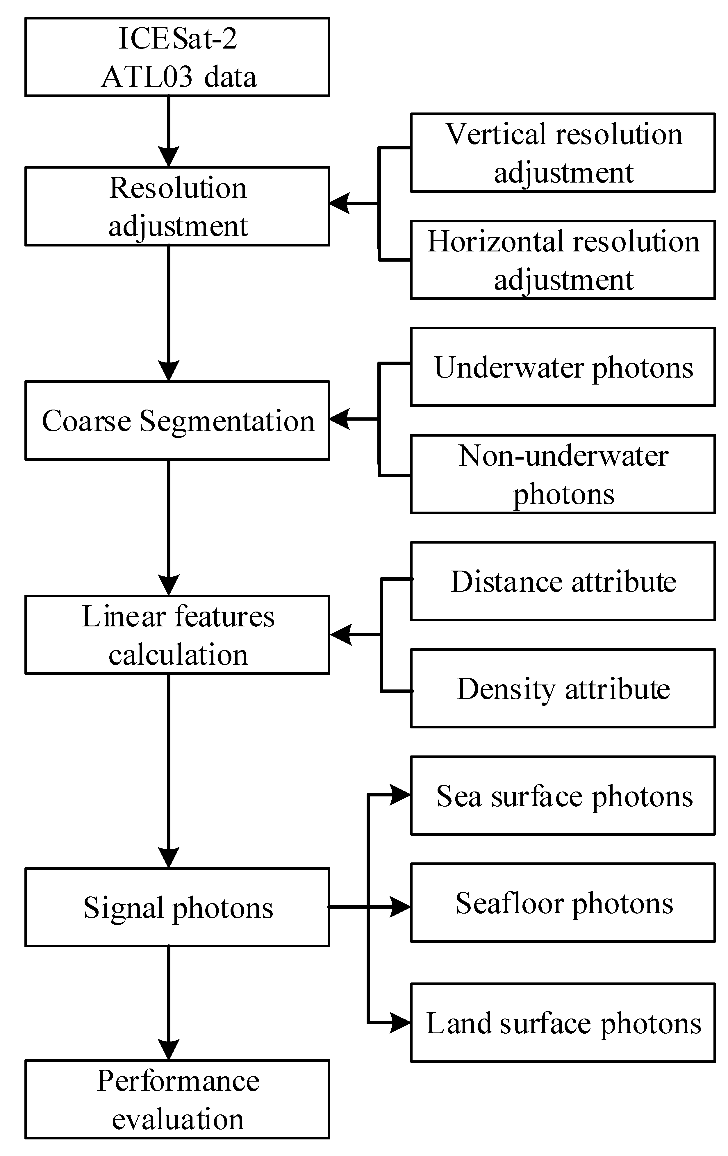
Based on these characteristics, this paper proposes the Linear Feature-Based Signal Photon Extraction (LFSPE) method to identify signal photons in ICESat-2 data. The LFSPE algorithm fully considers the spatial distribution differences and continuity characteristics of surface and seafloor photons and designs a comprehensive process for data preprocessing and signal extraction, as shown in Figure 2. This process includes four main steps: (1) resolution adjustment, optimizing vertical and horizontal resolutions to reduce redundant photons and standardize the data distribution characteristics; (2) coarse segmentation of underwater and non-underwater photons, using elevation histograms combined with Gaussian fitting for dynamic photon extraction; (3) signal photon identification, extracting signal photons based on their linear features and filtering out noise photons. Through these steps, the LFSPE algorithm can efficiently and accurately extract surface and seafloor photon signals, providing reliable support for shallow-water bathymetry and topographic analysis.

2.3.1. Data Resolution Adjustment

When the ICESat-2 satellite is operating, the ATLAS instrument emits laser pulses at a fixed frequency, with a wavelength of 532 nm. Each pulse can theoretically return multiple photons, meaning that a single laser spot may correspond to several photon signals. This can result in multiple photon data points with similar elevation values at the same horizontal position, as shown in Figure 3a. This situation can interfere with the calculation of neighborhood features for the photon data. To avoid this issue, the study first adjusts the vertical resolution of the raw photon data. The specific steps are as follows:
Step 1. Calculation of Along-Track Distance: Using the time information associated with the photon data, the along-track distance is calculated. The along-track distance is then shifted so that it starts from zero for easier subsequent processing.
Step 2. Grouping Photons by Pulse: Photons belonging to the same laser pulse are grouped together. As shown in Figure 3a, the photons within the ellipses belong to the same pulse.
Step 3. Euclidean Clustering: For each group of photons, Euclidean clustering is applied with a distance threshold of d m i n , which is set to 0.5 by default. This step assigns the photons into different clusters based on their spatial proximity.
Step 4. Cluster Point Selection: For each cluster, the median of the two-dimensional coordinates is calculated and serves as the reference point. The photon closest to the median point is selected as the “retained point” for that cluster. These retained points make up the new photon data after vertical resolution adjustment, as shown in Figure 3b.
Figure 3 provides a schematic of vertical resolution adjustment for the original photon data. The data shown in the figure is part of experimental dataset 8. The upper portion of the cyan line represents surface photons, while the lower portion represents seafloor photons, including noise photons. In Figure 3a,b, the photons inside the ellipses represent the photon data from the same laser spot before and after the vertical resolution adjustment. From the figure, it is clear that redundant photon data within the same laser spot are effectively removed.
During the operation of ICESat-2, photon data from different regions, times, and beams can have inconsistent horizontal resolutions, sometimes with significant differences. As photon data denoising algorithms are highly sensitive to horizontal resolution, this can lead to the need for re-tuning the algorithm for different datasets. To address this issue, preprocessing is required to standardize the horizontal resolution across datasets, ensuring that the photon data in different datasets have consistent or similar horizontal resolutions. Given that the ICESat-2 sampling rate is 10 kHz, with an approximately 0.7 m along-track resolution on the ground, the along-track distance between adjacent laser spots ( d t r a c k ) is adjusted to 0.7 m. For particularly sparse datasets, the distance between adjacent laser spots can be further reduced to ensure the continuous distribution of signal photons.

2.3.2. Segmentation of Underwater and Non-Underwater Photons

Some regions, such as experimental datasets 5, 6, and 8 in this study, have shallow and flat seawater depths. In these areas, the vertical distance between surface and seafloor photon signals is small. Without distinguishing between underwater and non-underwater photon data, the computed photon features may interfere with each other, ultimately affecting the identification of signal photons. Therefore, coarse segmentation of the photon data into underwater and non-underwater photons is beneficial for accurately identifying surface and seafloor photon signals in subsequent algorithms.
Photon distribution characteristics differ significantly between land, sea surface, and seafloor. Photon data fluctuate with terrain; however, due to seawater attenuation and the complex and variable nature of seafloor topography, seafloor photon data tends to be sparser compared to sea surface and land photons. In shallow-water regions with sufficient along-track distance, the number of photons returning from the sea surface is much greater than noise photons, underwater signal photons, and adjacent land photons. Therefore, using elevation histograms for coarse segmentation of sea surface and underwater photon data is a common method. However, previous elevation histogram methods may misclassify some seafloor photon data as sea surface or above-sea-level photons, particularly in shallow areas. This study proposes a new coarse segmentation method that accounts for both global and local sea surface elevations. The steps are as follows:
Step 1. The Y-coordinates of the experimental data are binned at 0.1 m intervals to create an elevation histogram, and Gaussian fitting is applied to obtain the parameters μ a l l and σ a l l of the Gaussian function:
f x = a × exp x μ 2 2 σ 2
where x is the center of each bin, f ( x ) is the data count in the bin, a is the amplitude, μ is the mean, and σ is the standard deviation.
Step 2. For the along-track data, the segment is divided every 200 m. Elevation histograms are then created for each segment with 0.1 m bins, and Gaussian fitting is performed to obtain μ b l o c k and σ b l o c k for each segment.
Step 3. If μ a l l μ b l o c k > 1 or σ b l o c k > 0.5 , the Gaussian fitting for the segment is considered insufficient to represent the sea surface. In this case, μ a l l and σ a l l are assigned to μ b l o c k and σ b l o c k .
Step 4. For each segment, photons with Y-coordinates satisfying y > μ b l o c k 4 σ b l o c k are classified as non-underwater photons; others are classified as underwater photons.
Step 5. Repeat steps 2, 3, and 4 to perform coarse segmentation of underwater and non-underwater photons, which will be used for subsequent signal photon identification.
Figure 4 illustrates the segmented Gaussian fitting for coarse segmentation, using data from experimental dataset 2. In Figure 4a, almost only surface photon data is present, and the standard deviation of the Gaussian model fitted to the elevation histogram is small. μ a l l and μ b l o c k are close, allowing μ b l o c k to be used directly for differentiating underwater and non-underwater photon data. In Figure 4b, seafloor photons are present in the elevation histogram, but their peak is smaller than that of the surface photons. Figure 4c shows land photons, where the difference between μ a l l and μ b l o c k is large, and σ b l o c k is also large. After assigning μ a l l to μ b l o c k , surface photons can be effectively distinguished. In Figure 4d, where the water depth is shallow, the sea surface and seafloor photons overlap. However, using the segmented elevation histogram and μ b l o c k , the sea surface and seafloor photons can be finely differentiated. Figure 4e shows that the peak for seafloor photons is larger than the peak for surface photons, but due to a significant difference between μ b l o c k and μ a l l , assigning μ a l l to μ b l o c k effectively separates underwater and non-underwater photons. Finally, Figure 4f illustrates seafloor topography with significant variations, and the elevation histogram of this segment exhibits multiple peaks. However, the sea surface peak is larger, allowing μ b l o c k to be used directly for distinguishing underwater and non-underwater photon data.

2.3.3. Extraction of Signal Photons

After the coarse segmentation process described above, signal photons are extracted from both the underwater and non-underwater photon data. Signal photons exhibit distinct linear or near-linear spatial distribution patterns in the data. These photons change continuously in horizontal or sloped directions, and in these directions, the photon density remains relatively uniform and is higher than that of noise photons. Additionally, the distance between adjacent signal photons is smaller. This study quantifies these features to distinguish signal photons from noise photons. The process for calculating the photon density and distance features based on linear characteristics is as follows:
Step 1. Set Variable Neighborhood Radius: For non-underwater photon data, a fixed neighborhood radius is used to obtain neighboring photons, while a variable neighborhood radius is used for underwater photon data feature calculation. The laser signal experiences exponential energy attenuation as it passes through water, causing the number of signal photons to decrease rapidly with depth. Fixed-radius neighborhood searches will lead to fewer photons being found at deeper underwater points, preventing correct photon feature calculations. To address this issue, a variable neighborhood search strategy is adopted, where the neighborhood radius gradually increases with increasing depth. The variable neighborhood radius r i is calculated using the following formula:
r i = r m i n + r m a x r m i n × h m a x h i h m a x h m i n
where r i is the variable neighborhood radius for the i -th photon, r m i n and r m a x are the lower and upper bounds of the neighborhood radius, h m i n and h m a x are the minimum and maximum elevation values of the photon data, and h i is the elevation value for the i -th photon.
In this study, the maximum elevation value of the underwater photon data is used as h m a x . Considering that the maximum laser penetration depth of ATLAS can exceed 30 m [28], the minimum elevation is set as h m i n = h m a x 30 . For photons with h i < h m i n , the neighborhood radius r = r m a x . For non-underwater photons, a fixed neighborhood radius r s e a r c h = 30 m is used. For underwater photons, the neighborhood search radius is r m i n = 20 m and r m a x = 50 m.
This depth-dependent adjustment reflects the signal attenuation effect observed in underwater photon returns. Although we do not explicitly calculate a physical attenuation coefficient, the gradual reduction in photon density with depth—caused by scattering and absorption in the water column—is implicitly modeled by expanding the neighborhood radius. This strategy ensures that the algorithm remains effective in detecting weak signal photons at greater depths.
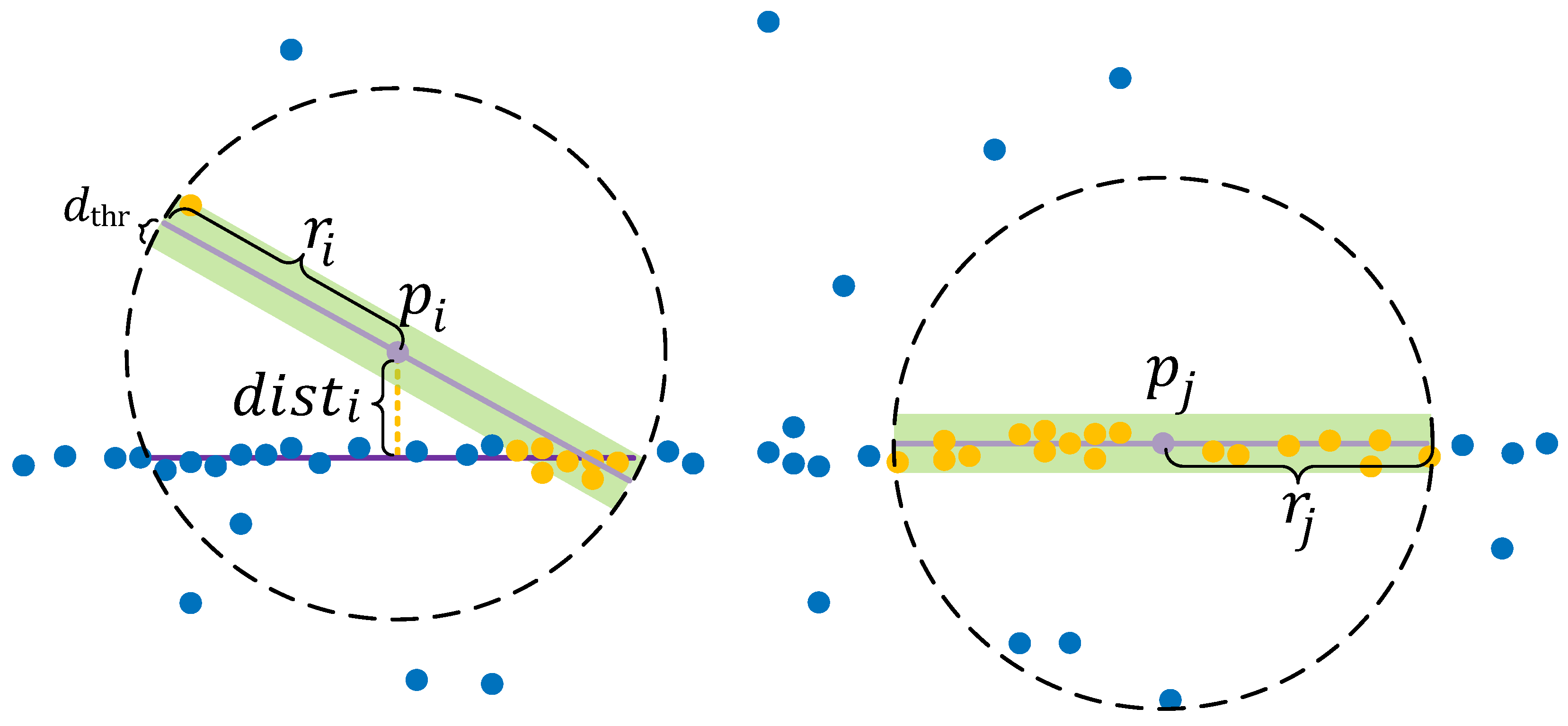
Step 2. Linear Feature Calculation: The KD-tree is constructed using the along-track distance and elevation values of the photon data. The neighborhood points for each photon p i are identified by searching within the radius r i . A straight line L (shown in purple in Figure 5) is fitted through the neighborhood points of p i , ensuring that as many points as possible from the neighborhood fall within a specified distance range d t h r from this line L (shown as the green rectangular area in Figure 5). The number of points within this green rectangle is counted as the density d e n s i t y i of point p i . Using the RANdom SAmple Consensus (RANSAC) algorithm, a straight line L R A N S A C (shown in purple in Figure 5) is fitted to the neighborhood points of p i , and the distance from point p i to this line L R A N S A C is calculated as d i s t i , the distance feature of the point p i . In this way, two linear features, density d e n s i t y i and distance d i s t i , are computed for each point p i .
Step 3. Signal Photon Recognition: Whether points p i and p j are signal points or noise points depends on the linear features d e n s i t y and d i s t calculated in step 2. From Figure 5, it can be observed that for signal photons, the density should be higher than that of noise points, and the distance should be smaller. Therefore, based on the point density and distance calculated in step 2, signal photons can be easily identified by setting thresholds d e n s i t y t h r and d i s t t h r . Points that satisfy the condition given in Equation (3) are classified as signal photons, while those that do not are considered noise photons.
signal i = 1 , if   density i > density thr   and   dist i < dist thr , 0 , otherwise .
where the s i g n a l i is set to 1 if the density i of p i exceeds the threshold density thr , and the distance dist i is less than the threshold dist thr . Otherwise, s i g n a l i is set to 0, indicating noise.

2.3.4. Refraction Correction

ATL03 elevation data has been corrected for atmospheric delay, solid tides, system pointing biases, and other factors. However, the depth measurement errors caused by refraction have not been corrected [29]. Refraction in water causes the displacement of photons at the seafloor, thereby reducing the accuracy of depth measurements [30,31]. When photons enter the ocean, they refract at the air–water interface, causing both horizontal and vertical displacements. This leads to an overestimation of the photon travel distance, making the seafloor appear deeper. At a water depth of around 30 m, refraction-induced depth measurement errors can reach 7 to 8 m, which is not negligible. To obtain more accurate seafloor topography data, it is necessary to correct the depth errors caused by refraction effects. In this study, we adopt a refraction correction method proposed by Parrish et al. [32], which is applicable under specific conditions (i.e., when a first-order approximation of refraction correction is acceptable, and the plane component can be ignored). The corrected seafloor photon elevation can be approximated using the following formula:
h = h 0 + 0.25416 × D
where h represents the corrected photon height, h 0 is the original height measurement, and D is the absolute depth from the water surface to the seafloor.

2.3.5. Evaluation Methodology

To quantitatively evaluate the accuracy of the signal photon extraction algorithm, the manually identified signal photons are considered as the true signal photons. The performance of the algorithm for extracting sea surface and seafloor photons is assessed using overall accuracy (OA), precision (P), recall (R), and F1 score. Precision (P) is defined as the proportion of correctly identified true signal photons among all extracted signal photons, while recall (R) represents the proportion of true signal photons that were correctly detected. The F1 score is the harmonic mean of precision and recall [16]. The formulas for these metrics are as follows:
O A = T P + T N T P + T N + F P + F N
P = T P T P + F P
R = T P T P + F N
F 1 = 2 × P × R P + R
where T P (True Positives) represents the number of true signal photons correctly identified; T N (True Negatives) is the number of noise photons correctly classified; F P (False Positives) refers to noise photons misclassified as signal photons; and F N (False Negatives) refers to true signal photons that were not detected.
Using the CUDEM bathymetric data, the coefficient of determination (R2), mean absolute error (MAE), and root mean square error (RMSE) were calculated to assess the agreement between the seafloor topography data derived from ICESat-2 and CUDEM. These metrics evaluate the fitting degree and error of the seafloor data. It should be noted that the seafloor topography data from ICESat-2 and CUDEM must be aligned to the same ellipsoidal reference before comparison. The formulas for these metrics are as follows:
R 2 = 1 i = 1 n y i y i 2 i = 1 n y i y ¯ 2
M A E = 1 n i = 1 n y i y i
R M S E = 1 n i = 1 n y i y i 2
where y i is the water depth derived from ICESat-2 data; y i is the water depth from CUDEM; y ¯ is the mean value of the measured water depth; and n is the total number of water depth points extracted from ICESat-2 data.

3. Results

3.1. Parameter Selection

In the proposed method, parameters are categorized into insensitive and sensitive types. Insensitive parameters are those whose settings remain consistent across different experimental datasets. Sensitive parameters, however, require appropriate adjustments based on the dataset. For non-underwater data, all parameters can be set to the default values provided in Section 3.3. For underwater photons, particularly in the process of identifying seafloor topography, certain parameters need to be adjusted according to the dataset.
During the resolution adjustment phase, the along-track distance ( d t r a c k ) is classified as a sensitive parameter. In the signal photon identification phase, the density threshold ( d e n s i t y t h r ) and distance threshold ( dist thr ) are also sensitive parameters. Table 2 details the settings of these sensitive parameters for the proposed algorithm. For nighttime data, d t r a c k is set to 0.7 m. However, for daytime data, where signal photons are often obscured by noise photons, the d t r a c k requires adjustment to enhance the continuity of signal photons.
The d e n s i t y t h r is typically set within the range of 20 to 37. This parameter correlates with changes in d t r a c k : smaller d t r a c k values result in higher calculated density values, necessitating corresponding adjustments to d e n s i t y t h r . In most cases, dist thr is set between 0 and 3 m to effectively identify signal photons. For dataset 8, however, dist thr is set to 7 m to capture a few signal photons at greater depths.
We employed MATLAB 2022a’s built-in RANSAC function for robust linear fitting when computing local linear features. A minimal sample size of 2 was used, which is appropriate for 2D line fitting. The maximum number of iterations and the confidence level were both set to their default values—1000 trials and 99% confidence, respectively.

3.2. Underwater and Non-Underwater Photon Segmentation Results

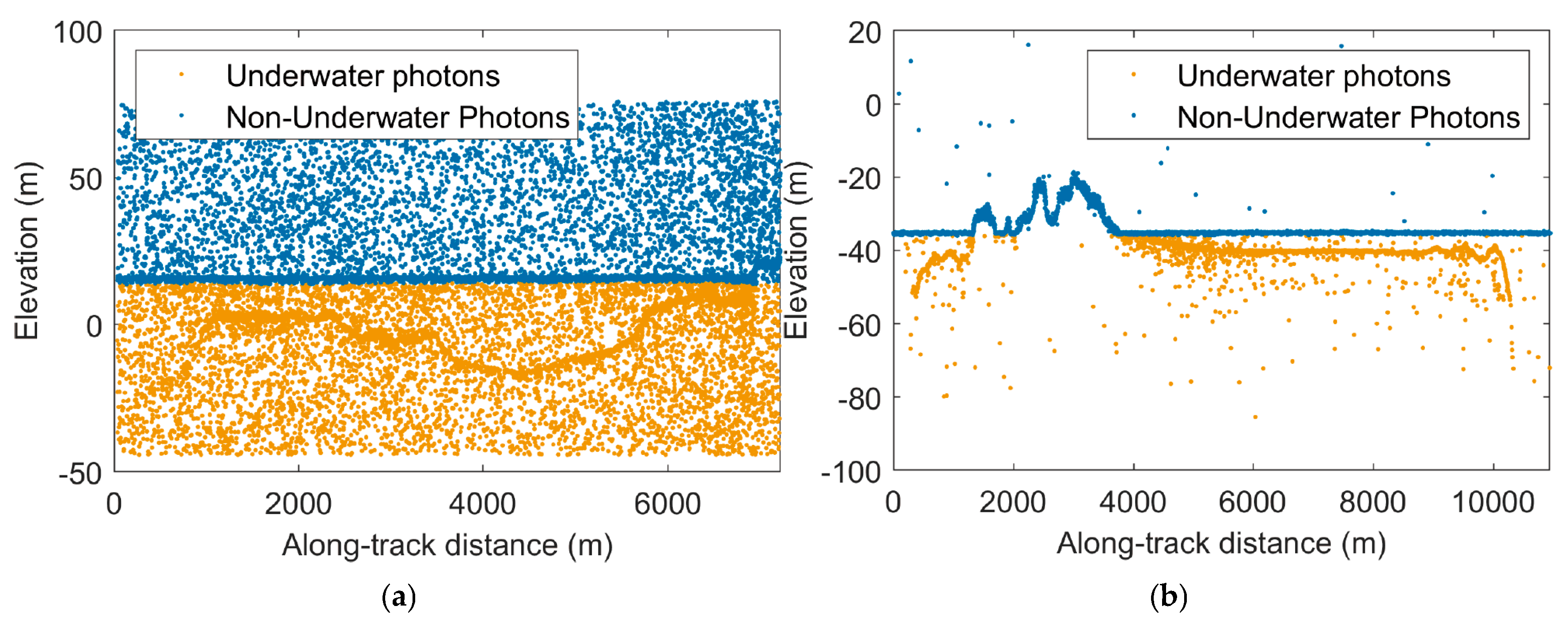
Figure 6 illustrates the results of the coarse segmentation algorithm described in Section 2.3.2 applied to ICESat-2 photon data, distinguishing underwater photons (orange points) from non-underwater photons (blue points). Panels (a) to (h) correspond to datasets 1 through 8 in Table 1. The results demonstrate that the coarse segmentation algorithm effectively performs signal photon extraction tasks under various regional and environmental conditions, exhibiting robustness and accuracy.
In Figure 6a,c,d,f, which depict daytime photon data, the number of noise photons is significantly higher compared to the nighttime datasets shown in Figure 6b,e,g,h. Among the daytime datasets, underwater photons are often connected to terrestrial photons, particularly in coastal regions. The photon data exhibit distinct stratification, indicating that the coarse segmentation algorithm effectively distinguishes between surface and underwater photons in land–sea transitional zones.
Figure 6e covers the longest track length (approximately 16,000 m), encompassing areas with varying seafloor slopes and water depths. Even in regions where the vertical distance between the sea surface and the seafloor photons is minimal, the coarse segmentation algorithm maintains its effectiveness in distinguishing underwater and non-underwater photons.
Figure 6f,g demonstrate areas with shallow-water depths and long-range flat seafloor terrains, while Figure 6h illustrates seafloor regions with significant elevation variation. The algorithm produces clear and well-defined segmentation boundaries in these regions, further demonstrating its reliability.

3.3. Extraction Results of Signal Photons

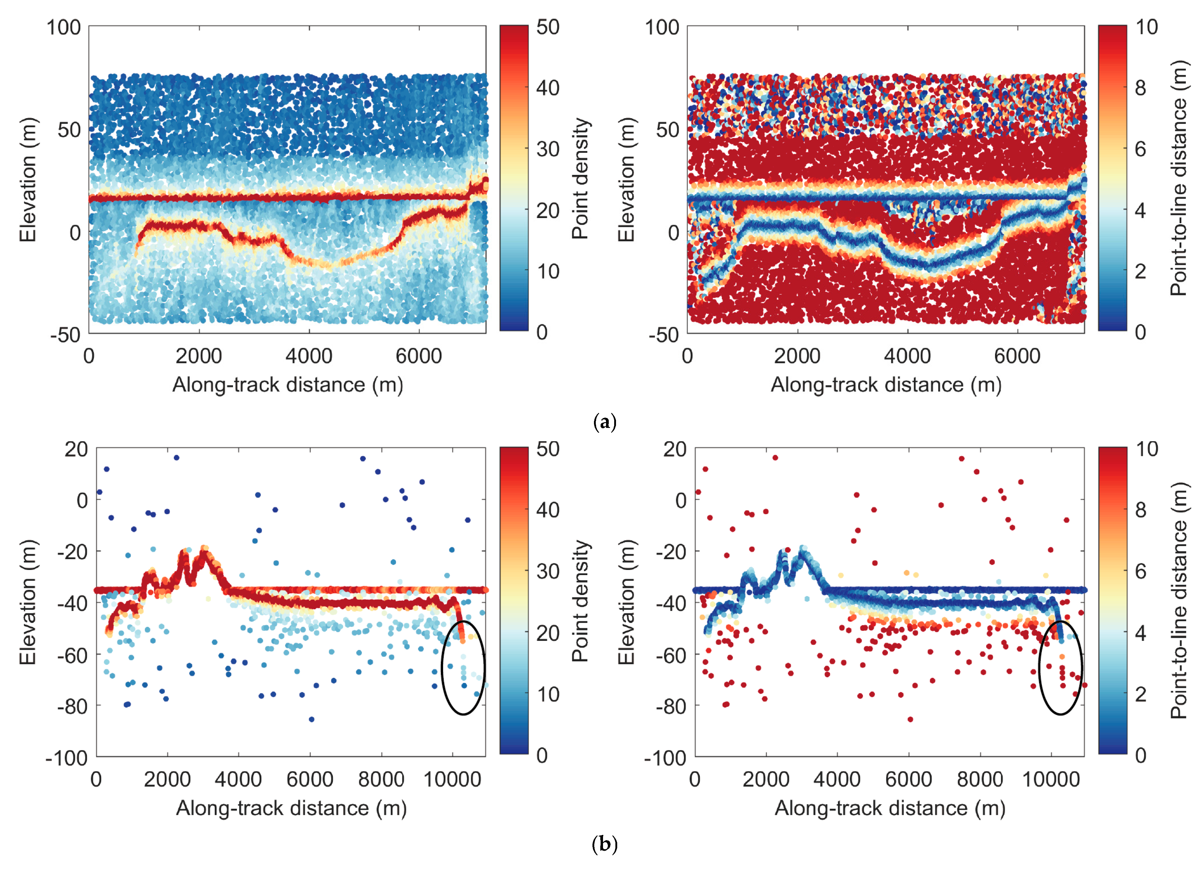
Figure 7a–h illustrate the linear features of photon data from experimental areas 1 to 8, with the left column showing density maps and the right column showing distance maps. These figures clearly demonstrate the significant differences in linear features between signal photons (e.g., sea surface, seafloor, and land photons) and noise photons. Signal photons exhibit significantly higher density values and lower distance values compared to noise photons.
The density maps (left column) depict the distribution patterns of photon density along the track direction. Surface photons maintain consistently high-density levels, reflecting their regular and continuous distribution along the track. In contrast, the density of land photons is influenced by terrain slope and vegetation cover, as shown in Figure 7b–d,g. For seafloor photons, even with dynamically adjusted neighborhood search radii to account for increasing depth, their density decreases markedly with increasing water depth. In deeper water regions, signal photons become sparse and eventually disappear, as observed in the terminal regions of Figure 7b,h.
The distance maps (right column) reveal the distribution of distances between photons and the line L R A N S A C for their neighborhood point sets, reflecting the spatial linearity of signal photons. Overall, surface photons, characterized by their regularity and continuity, exhibit smaller distances to the fit line L R A N S A C , typically ranging between 0 and 1. This indicates strong linearity and consistency in surface photons. Seafloor photons, however, are affected by factors such as water depth, terrain variability, and density attenuation, resulting in larger distances, generally within the range of 0 to 3. In shallow-water regions, seafloor photons exhibit higher density and smaller distances, while in deeper regions, the distance distribution becomes more variable, as highlighted by the ellipses in Figure 7b,h.
Figure 8 compares the extraction performance of the proposed method (left column) with the DBSCAN algorithm (right column) across the eight experimental areas. In the figures, black points denote noise photons, orange points represent identified seafloor photons, blue points indicate sea surface photons, and green points correspond to land photons. The results demonstrate that the proposed method effectively identifies seafloor photons in sparse photon regions, even in deeper-water regions, as highlighted in the magnified region of Figure 8a. In shallow-water regions, the boundaries between seafloor and surface photons are clearer, as shown in the magnified region of Figure 8b. Additionally, the proposed method exhibits robust performance in sparse or complex photon regions, capturing more underwater photons, as demonstrated in the magnified region of Figure 8e.
In contrast, the DBSCAN algorithm shows significant shortcomings. As water depth increases, DBSCAN often fails to detect many seafloor photons. For surface photons, DBSCAN frequently misclassifies noise photons near the surface as signal photons, as illustrated in Figure 8a.

3.4. Evaluation of Signal Photon Extraction Accuracy

To quantitatively evaluate the performance of the proposed method, a manually annotated reference dataset was created. Manual labeling was performed using PhotonLabeling, a custom-developed interactive software designed for ICESat-2 photon data annotation. Signal photons were identified through visual inspection based on their spatial continuity, depth progression, and local density. Annotation consistency was ensured through cross-validation and consensus. The PhotonLabeling tool used for this process is publicly available for download at: https://github.com/zwshi-pku/PhotonLabeling (accessed on 5 August 2025).
A statistical analysis of the seafloor photon extraction results across eight datasets was conducted. The results demonstrate that the proposed algorithm consistently achieved high accuracy across diverse scenarios. The average precision, recall, F1 score, and overall accuracy were 0.977, 0.958, 0.967, and 0.972, respectively. Notably, precision exceeded 0.96 for all datasets, reflecting the method’s strong ability to suppress noise photons. Recall values surpassed 0.90 in most datasets, particularly in high-density photon environments such as datasets 2 and 8, where recall reached 0.985 and 0.997, respectively. The highest F1 scores were also observed in these datasets, peaking at 0.986 (dataset 2) and 0.985 (dataset 8). Overall accuracies exceeded 0.97 in five of the eight datasets, with a maximum of 0.990. These results are summarized in Table 3, confirming the robustness and generalization capability of the proposed algorithm under varying photon densities and seafloor complexity.
Compared to the DBSCAN algorithm, which achieved a precision of 0.751, a recall of 0.817, a F1 score of 0.778, and an overall accuracy of 0.796, the proposed method demonstrated substantial improvements across all evaluation metrics. Specifically, precision increased by 30.0%, recall by 17.3%, F1 score by 24.3%, and overall accuracy by 22.2%.

3.5. Performance Evaluation Across Different Water Depth Intervals

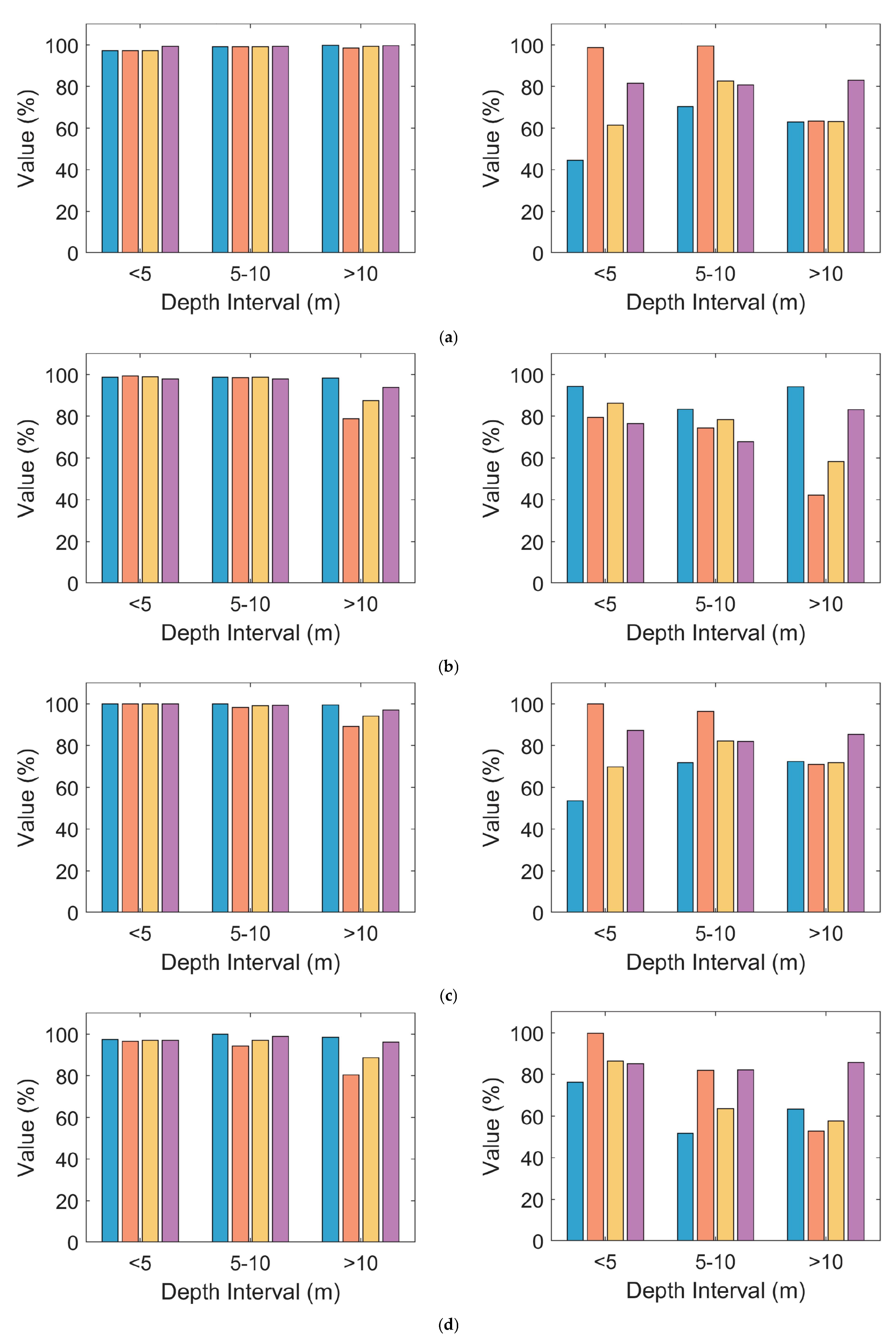
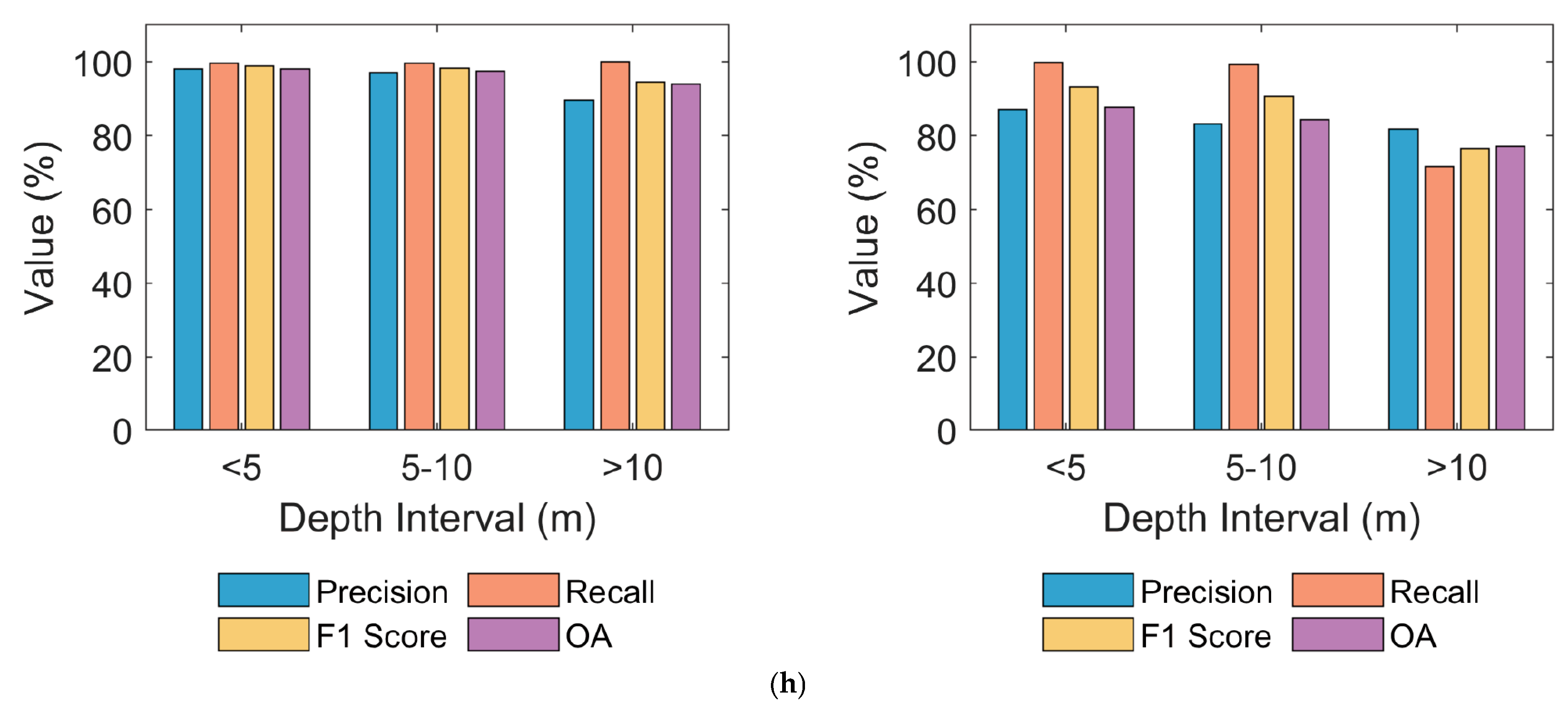
To evaluate the robustness and adaptability of the proposed LFSPE algorithm under varying water depths, the experimental data were divided into three depth intervals: 0–5 m, 5–10 m, and greater than 10 m. Four standard metrics—precision, recall, F1 score, and overall accuracy—were calculated for each of the eight experimental regions.
Figure 9 illustrates the performance of the proposed method (left panel) and the comparison algorithm DBSCAN (right panel) across the eight experimental regions (a–h). It can be observed that the proposed method consistently achieves high scores across all depth intervals, with only minor performance degradation as depth increases. This demonstrates the algorithm’s strong adaptability in scenarios with sparse signal photons and high noise levels.
In contrast, DBSCAN exhibits significant variations in performance across different depths, mainly due to its tendency to misclassify a large number of noise photons as signal photons while missing many actual signal photons. The performance drop in the >10 m interval is particularly notable, indicating its limited ability to handle photon density variations across depth. These results confirm the robustness of the proposed method in complex seafloor topographies and deeper-water regions.
To further contextualize our results, we note that Huang, Dong, Liu, Chen, Li, Wang and Meng [28] proposed a photon denoising method that accounts for heterogeneous density and weak connectivity. According to their published results (see Figure 14 in [28]), signal extraction performance declines more substantially in deeper waters (depth > 10 m). In contrast, the proposed LFSPE method maintains relatively stable and high accuracy across all depth intervals, including those exceeding 10 m. This comparison suggests that our approach may offer enhanced robustness and reliability in photon-limited or high-noise underwater environments.

3.6. Bathymetric Accuracy Evaluation

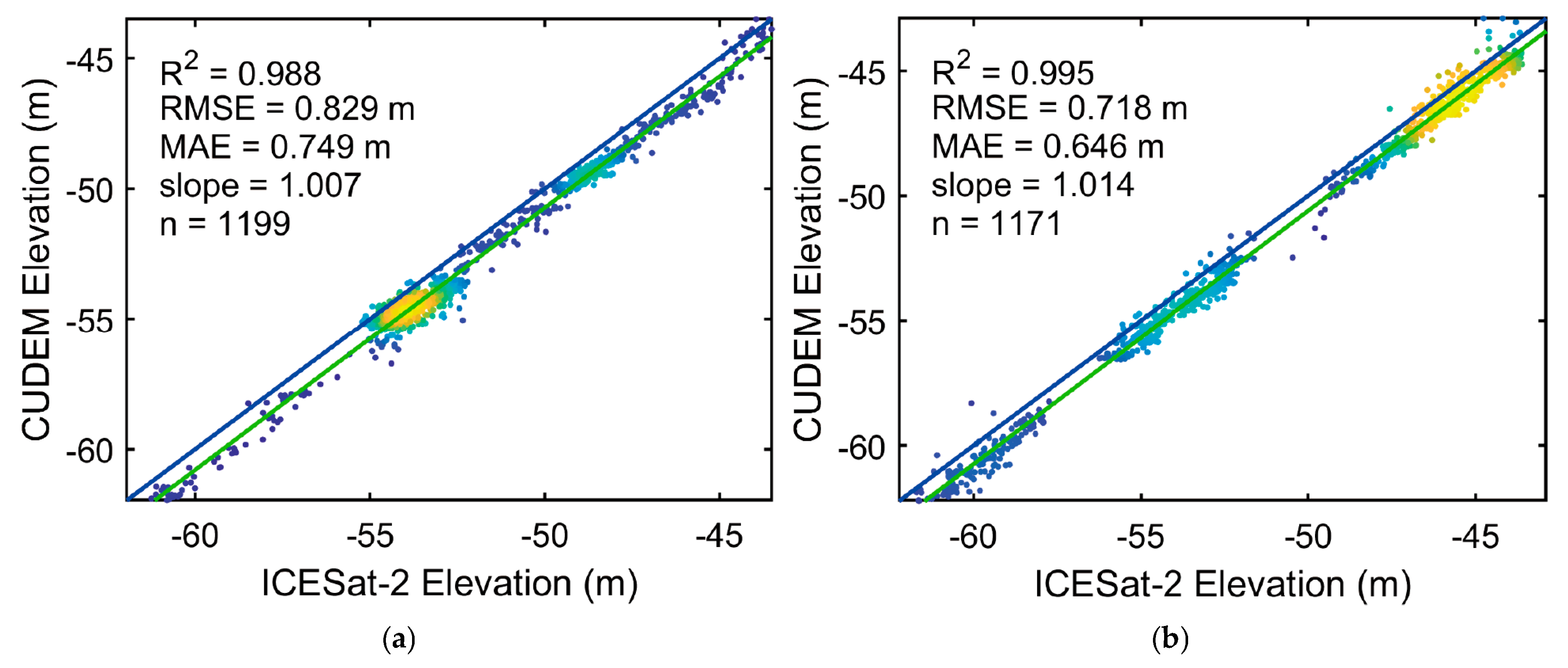
To further validate the accuracy of the proposed seafloor signal photon extraction method, the extracted results were compared with a high-resolution reference dataset—CUDEM. Since only experimental regions 3 and 4 in the dataset are accompanied by CUDEM elevation data, this section focuses on evaluating the bathymetric accuracy for these two regions, as shown in Figure 10a,b.
The comparison with CUDEM data demonstrates a strong consistency between the bathymetric results extracted from ICESat-2 data and the CUDEM elevation model. The correlation coefficients R2 for experimental regions 3 and 4 reached 0.988 and 0.995, respectively, indicating a high degree of linear correlation. This suggests that the proposed method accurately captures depth variation trends, even in complex topographic environments. Specifically, the root mean square error (RMSE) was 0.829 m and 0.718 m for experimental regions 3 and 4, respectively, while the mean absolute error (MAE) was 0.749 m and 0.646 m. The slopes of the regression lines were 1.007 and 1.014 for experimental areas 3 and 4, respectively, further demonstrating the precision and consistency of the method in complex terrain.
The comparative evaluation with CUDEM data substantiates the effectiveness of the proposed method for seafloor photon extraction and bathymetric measurement. High R2 values, along with low RMSE and MAE values, indicate that the method reliably provides accurate seafloor photon extraction results.

4. Discussion

4.1. Sensitivity Analysis of Algorithm Parameters

The parameters in the proposed algorithm are categorized into two types: non-sensitive parameters and sensitive parameters. Non-sensitive parameters are those that remain consistent across all eight experimental datasets, while sensitive parameters require adjustment according to the specific characteristics of the data to achieve optimal signal photon extraction.
In the vertical resolution adjustment phase, a smaller d m i n value can lead to over-clustering, retaining redundant photons, whereas a larger d m i n may result in the loss of signal photons. This issue is particularly pronounced in shallow-water regions, where excessive d m i n values may cause the omission of sea surface and seafloor signal photons. Therefore, d m i n must be set to a value smaller than the shallow-water depth. In this study, d m i n is consistently set to 0.5 m, making it a non-sensitive parameter across all datasets.
In the horizontal resolution adjustment phase, the along-track interval d t r a c k significantly influences datasets with varying photon density distributions. Adjusting d t r a c k ensures that the algorithm’s linear feature thresholds remain adaptable. Larger intervals may reduce the continuity of signal photons, while smaller intervals (<0.5 m) increase sensitivity to noise photons. For datasets with significant noise (e.g., daytime data), a smaller d t r a c k can mitigate signal photon suppression by noise. Conversely, nighttime datasets perform well with default settings. For sparse seafloor photons, reducing d t r a c k helps maintain signal continuity.
During the coarse segmentation phase, the algorithm employs a segmented single-Gaussian fitting approach to classify photons. This segmentation avoids failure in regions with long along-track distances, large datasets, or significant terrain undulations. After segmentation, seafloor slopes with gradually increasing depth (Figure 4a) allow Gaussian fitting to determine segmentation thresholds, distinguishing surface from seafloor photons. In nearly parallel seafloor and surface scenarios, the histogram reflects two peaks, where the surface photon peak is higher and at a greater elevation. Gaussian fitting can leverage this feature for segmentation (Figure 4b). When the seafloor peak surpasses the surface peak (Figure 4c), overall Gaussian fitting constrains the segmentation results for accurate segmentation. Without segmentation, coarse segmentation may fail in shallow-water and coastal transition zones, such as in experimental areas 5, 6, and 8. The global Gaussian model serves as a reference baseline for the approximate sea surface elevation across the entire track. Local Gaussian models are fitted to segmented photon subsets for finer-scale surface detection. The consistency between local and global estimates is evaluated, and significant deviations are flagged to reduce false sea surface identification due to local anomalies. This integration strategy enhances segmentation robustness without requiring numerical fusion of the two models. By combining global and local Gaussian models, the proposed method provides a robust approach to segmenting underwater and non-underwater photons, adapting to variations in water surface elevation along the track.
In the signal photon extraction phase, the density threshold ( d e n s i t y t h r ) represents the minimum density required for a photon to be classified as a signal photon. Setting d e n s i t y t h r too low results in misclassification of noise photons as signal photons, reducing precision. Conversely, setting d e n s i t y t h r too high leads to the omission of sparse signal photons, particularly in low-density datasets. Based on experimental results, an optimal range of 20 ≤ d e n s i t y t h r ≤ 37 strikes a balance between minimizing misclassification and retaining true signals.
The distance threshold ( dist thr ) measures the maximum allowable deviation of a photon from the line L R A N S A C . A smaller dist thr excludes true signal photons with minor deviations caused by noise or irregular terrain, while a larger dist thr includes more noise photons, reducing precision. Experimental results show that an optimal dist thr range of 1–3 effectively extracts signal photons from noise photons.
Both d e n s i t y t h r and dist thr can be determined using linear feature maps. For most datasets, these thresholds remain consistent, but in sparse seafloor photon cases, adjustments may be necessary to accommodate specific conditions. Specifically, the density and distance maps shown in Figure 7 reveal distinct separation patterns between signal and noise photons, which serve as intuitive references for threshold selection. By examining the local density peaks and distance decay trends of known signal photon clusters, we identify a suitable range for each threshold that avoids over-segmentation while preserving true signal structures. This empirical approach allows flexible adaptation to diverse photon profiles while maintaining consistency in classification criteria across experiments.
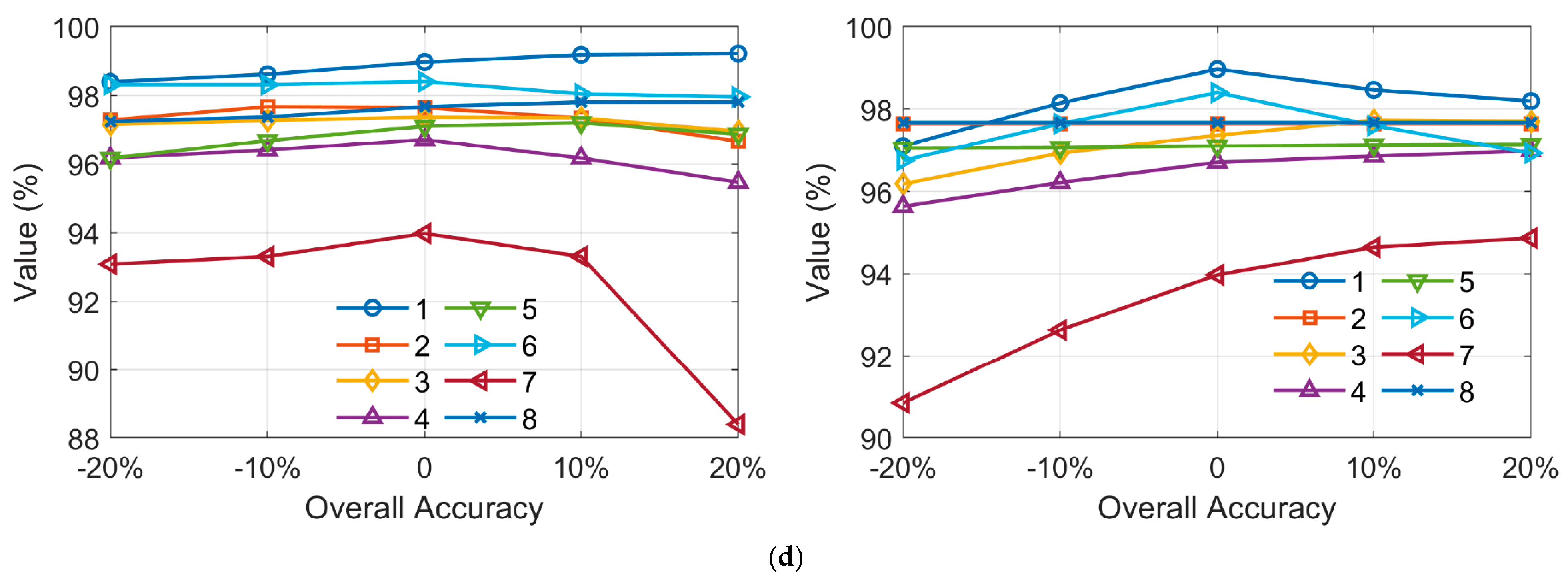
To evaluate the robustness of the proposed method to key parameter variations, we conducted a sensitivity analysis focusing on two critical parameters: d e n s i t y t h r and dist thr . While d_track is also involved in the algorithm design, its influence is coupled with d e n s i t y t h r and dist thr . Therefore, we isolate the effects of d e n s i t y t h r and dist thr by varying each independently within a ±20% range, while keeping other parameters fixed. Figure 11 illustrates the variations in precision, recall, F1 score, and overall accuracy across all eight datasets. The left column shows the results for d e n s i t y t h r , and the right column shows the results for dist thr .
The results reveal that the LFSPE algorithm maintains high performance under moderate parameter perturbations. When d e n s i t y t h r varies, the lowest observed metrics across all datasets are: precision 95.230%, recall 80.545%, F1 score 88.841%, and overall accuracy 88.393%. In comparison, for dist thr , the minimum metrics are: precision 93.326%, recall 84.276%, F1 score 90.852%, and overall accuracy 90.848%. These results indicate that the algorithm exhibits slightly greater sensitivity to d e n s i t y t h r , particularly in terms of recall.
Additionally, it can be observed that datasets 3, 4, and 7 are more sensitive to parameter changes than the others. These datasets show more pronounced performance degradation under both increased and decreased thresholds, likely due to their lower signal-to-noise ratio or more complex underwater topography. Overall, the analysis confirms that while parameter tuning can affect performance, the algorithm remains robust within a reasonable range.

4.2. Detection Capability of the Proposed Method

The traditional DBSCAN denoising algorithm requires extensive parameter tuning, particularly for the neighborhood radius ( e p s i l o n ) and the minimum number of points ( m i n p t ), to achieve satisfactory results. As shown in the right column of Figure 8, DBSCAN necessitates dataset-specific parameter adjustments to match the distribution characteristics of different ICESat-2 datasets, making the process time-consuming and complex. In contrast, the proposed method simplifies this challenge by using fixed parameters during the preprocessing stage, irrespective of the experimental region. This consistency significantly reduces the complexity of parameter adjustments. Furthermore, the signal photon extraction phase employs a parameter visualization approach based on photon linear features, streamlining the configuration process.
When handling high-noise or sparse photon data, DBSCAN often underperforms. As illustrated in Figure 8a, DBSCAN struggles to adapt to the significant differences in signal photon density between shallow and deeper-water regions, leading to suboptimal identification of signal photons. For surface photons, DBSCAN tends to misclassify noise photons near the signal photons as surface photons, further compromising its performance.

5. Conclusions

This study introduces a Linear Feature-Based Signal Photon Extraction (LFSPE) method for signal photon extraction and bathymetric retrieval using ICESat-2 ATL03 data. The LFSPE algorithm combines adaptive resolution adjustment, segmented Gaussian fitting, and linear feature analysis to effectively address challenges posed by high noise, sparse photon densities, and complex terrains. The validation conducted on eight different datasets demonstrates the robustness of the algorithm, with average precision and recall exceeding 0.97 and 0.95, respectively. The average F1 score and overall accuracy both surpass 0.96. Additionally, comparisons with CUDEM high-resolution bathymetric data confirmed the accuracy of the extracted bathymetric results, with R 2 values up to 0.98 and RMSE as low as 0.83 m.
The LFSPE method provides a reliable and adaptive solution for signal photon extraction and shallow-water bathymetry, outperforming traditional approaches in challenging environments. Its ability to maintain high performance across diverse conditions highlights its potential for advancing marine surveying and environmental monitoring.

Author Contributions

Conceptualization, Z.S. and J.L.; methodology, Z.S. and H.L.; software, Z.Y. and X.L.; validation, Z.S., J.L. and H.C.; formal analysis, Z.Y. and S.Z.; investigation, Z.S. and H.L.; resources, Q.L. and H.C.; data curation, Z.S. and S.Z.; writing—original draft preparation, Z.S.; writing—review and editing, Z.S. and Q.L.; visualization, Z.S. and S.Z.; supervision, Z.S. and H.L.; project administration, H.L.; funding acquisition, Z.S. All authors have read and agreed to the published version of the manuscript.

Funding

This research was financially supported by the National Natural Science Foundation of China (NSFC), Grant No. Y980650J30, with a total funding amount of CNY 300,000.

Data Availability Statement

The ICESat-2 ATL03 data utilized in this study were obtained from NASA’s Earthdata Search platform and are publicly accessible at https://search.earthdata.nasa.gov (accessed on 5 August 2025). The CUDEM bathymetric data, used as reference elevation data, were acquired from the NOAA and are available at https://www.ngdc.noaa.gov/mgg/bathymetry/bathymetry.html (accessed on 5 August 2025). Data preprocessing and baseline alignment were conducted using NOAA’s baseline conversion tools. To facilitate reproducibility, the source code for the proposed LFSPE algorithm, along with sample datasets, are publicly available at https://github.com/zwshi-pku/LFSPE-ICESat2-Bathymetry (accessed on 5 August 2025).

Acknowledgments

The authors express their sincere gratitude to NASA for providing the ICESat-2 ATL03 datasets, which were accessed through the Earthdata Search platform. Additionally, the authors acknowledge the NOAA for the provision of the CUDEM bathymetric data.

Conflicts of Interest

No potential conflict of interest was reported by the authors.

References

  1. Cao, B.; Wang, J.; Hu, Y.; Lv, Y.; Yang, X.; Gong, H.; Li, G.; Lu, X. ICESAT-2 Shallow Bathymetric Mapping Based on a Size and Direction Adaptive Filtering Algorithm. IEEE J. Sel. Top. Appl. Earth Obs. Remote Sens. 2023, 16, 6279–6295. [Google Scholar] [CrossRef]
  2. Louvart, P.; Cook, H.; Smithers, C.; Laporte, J. A New Approach to Satellite-Derived Bathymetry: An Exercise in Seabed 2030 Coastal Surveys. Remote Sens. 2022, 14, 4484. [Google Scholar] [CrossRef]
  3. Albright, A.; Glennie, C. Nearshore Bathymetry From Fusion of Sentinel-2 and ICESat-2 Observations. IEEE Geosci. Remote Sens. Lett. 2021, 18, 900–904. [Google Scholar] [CrossRef]
  4. Holman, R.; Haller, M.C. Remote Sensing of the Nearshore. Annu. Rev. Mar. Sci. 2013, 5, 95–113. [Google Scholar] [CrossRef] [PubMed]
  5. Traganos, D.; Poursanidis, D.; Aggarwal, B.; Chrysoulakis, N.; Reinartz, P. Estimating Satellite-Derived Bathymetry (SDB) with the Google Earth Engine and Sentinel-2. Remote Sens. 2018, 10, 859. [Google Scholar] [CrossRef]
  6. Song, Y.; Ma, Y.; Zhou, Z.; Yang, J.; Li, S. Signal Photon Extraction and Classification for ICESat-2 Photon-Counting Lidar in Coastal Areas. Remote Sens. 2024, 16, 1127. [Google Scholar] [CrossRef]
  7. Forfinski-Sarkozi, N.; Parrish, C. Analysis of MABEL Bathymetry in Keweenaw Bay and Implications for ICESat-2 ATLAS. Remote Sens. 2016, 8, 772. [Google Scholar] [CrossRef]
  8. Babbel, B.J.; Parrish, C.E.; Magruder, L.A. ICESat-2 Elevation Retrievals in Support of Satellite-Derived Bathymetry for Global Science Applications. Geophys. Res. Lett. 2021, 48, e2020GL090629. [Google Scholar] [CrossRef]
  9. Chen, Y.; Le, Y.; Zhang, D.; Wang, Y.; Qiu, Z.; Wang, L. A photon-counting LiDAR bathymetric method based on adaptive variable ellipse filtering. Remote Sens. Environ. 2021, 256, 112326. [Google Scholar] [CrossRef]
  10. Wang, B.; Ma, Y.; Zhang, J.; Zhang, H.; Zhu, H.; Leng, Z.; Zhang, X.; Cui, A. A noise removal algorithm based on adaptive elevation difference thresholding for ICESat-2 photon-counting data. Int. J. Appl. Earth Obs. Geoinf. 2023, 117, 103207. [Google Scholar] [CrossRef]
  11. Xie, H.; Xu, Q.; Luan, K.; Sun, Y.; Liu, X.; Guo, Y.; Li, B.; Jin, Y.; Liu, S.; Tong, X. Evaluating ICESat-2 Seafloor Photons by Underwater Light-Beam Propagation and Noise Modeling. IEEE Trans. Geosci. Remote Sens. 2024, 62, 4203018. [Google Scholar] [CrossRef]
  12. Gleason, A.C.R.; Smith, R.; Purkis, S.J.; Goodrich, K.; Dempsey, A.; Mantero, A. The Prospect of Global Coral Reef Bathymetry by Combining Ice, Cloud, and Land Elevation Satellite-2 Altimetry With Multispectral Satellite Imagery. Front. Mar. Sci. 2021, 8, 694783. [Google Scholar] [CrossRef]
  13. Coveney, S.; Monteys, X.; Hedley, J.D.; Castillo-Campo, Y.; Kelleher, B. ICESat-2 Marine Bathymetry: Extraction, Refraction Adjustment and Vertical Accuracy as a Function of Depth in Mid-Latitude Temperate Contexts. Remote Sens. 2021, 13, 4352. [Google Scholar] [CrossRef]
  14. Liu, J.; Liu, J. Analysis and comparison of denoising methods for photon-counting laser data. In Proceedings of the 2022 3rd International Conference on Geology, Mapping and Remote Sensing (ICGMRS), Zhoushan, China, 22–24 April 2022; pp. 175–178. [Google Scholar]
  15. Liu, A.; Cheng, X.; Chen, Z. Performance evaluation of GEDI and ICESat-2 laser altimeter data for terrain and canopy height retrievals. Remote Sens. Environ. 2021, 264, 112571. [Google Scholar] [CrossRef]
  16. Xie, J.; Zhong, J.; Mo, F.; Liu, R.; Li, X.; Yang, X.; Zeng, J. Denoising and Accuracy Evaluation of ICESat-2/ATLAS Photon Data for Nearshore Waters Based on Improved Local Distance Statistics. Remote Sens. 2023, 15, 2828. [Google Scholar] [CrossRef]
  17. Hui, Z.; Zhang, L.; Jin, S.; Chen, W.; Cheng, P.; Ziggah, Y.Y. Progressive noise photons removal from ICESAT-2 data based on the characteristics of different types of noise. GIScience Remote Sens. 2025, 62, 2507985. [Google Scholar] [CrossRef]
  18. Meng, W.; Li, J.; Tang, Q.; Xu, W.; Dong, Z. ICESat-2 laser data denoising algorithm based on a back propagation neural network. Appl. Opt. 2022, 61, 8395–8404. [Google Scholar] [CrossRef]
  19. Leng, Z.H.; Zhang, J.; Ma, Y.; Zhang, J.Y.; Zhu, H.T. A novel bathymetry signal photon extraction algorithm for photon-counting LiDAR based on adaptive elliptical neighborhood. Int. J. Appl. Earth Obs. Geoinf. 2022, 115, 17. [Google Scholar] [CrossRef]
  20. Surisetty, V.A.K.; Rajput, P.; Ramakrishnan, R.; Venkateswarlu, C. Synergistic Fusion of ICESat-2 Lidar and Sentinel-2 Data to Leverage Potential Mapping of Bathymetry in Remote Islands Using SVR. J. Indian Soc. Remote Sens. 2023, 51, 361–369. [Google Scholar] [CrossRef]
  21. Wang, Z.; Nie, S.; Wang, C.; Fu, B.; Xi, X.; Yang, B. A novel bathymetric signal extraction method for photon-counting LiDAR data based on adaptive rotating ellipse and curve iterative fitting. Int. J. Appl. Earth Obs. Geoinf. 2024, 132, 104042. [Google Scholar] [CrossRef]
  22. Li, N.; Wang, M.; Yang, B.; Pan, J.; Pi, Y.; Fan, Z. SCBMLD: A photon signal extraction method for ICESat-2 satellite-derived bathymetry. Opt. Express 2025, 33, 9023. [Google Scholar] [CrossRef]
  23. Lin, Y.; Jensen Knudby, A. Global automated extraction of bathymetric photons from ICESat-2 data based on a PointNet++ model. Int. J. Appl. Earth Obs. Geoinf. 2023, 124, 103512. [Google Scholar] [CrossRef]
  24. Velikova, M.; Fernandez-Diaz, J.; Glennie, C. ICESat-2 noise filtering using a point cloud neural network. ISPRS Open J. Photogramm. Remote Sens. 2024, 11, 100053. [Google Scholar] [CrossRef]
  25. Sarker, I.H. Deep Learning: A Comprehensive Overview on Techniques, Taxonomy, Applications and Research Directions. SN Comput. Sci. 2021, 2, 420. [Google Scholar] [CrossRef] [PubMed]
  26. Ratner, A.J.; De Sa, C.M.; Wu, S.; Selsam, D.; Ré, C. Data programming: Creating large training sets, quickly. Adv. Neural Inf. Process. Syst. 2016, 29, 3567–3575. [Google Scholar]
  27. Amante, C.J.; Love, M.; Carignan, K.; Sutherland, M.G.; MacFerrin, M.; Lim, E. Continuously Updated Digital Elevation Models (CUDEMs) to Support Coastal Inundation Modeling. Remote Sens. 2023, 15, 1702. [Google Scholar] [CrossRef]
  28. Huang, G.; Dong, Z.; Liu, Y.; Chen, Y.; Li, J.; Wang, Y.; Meng, W. An optimized denoising method for ICESat-2 photon-counting data considering heterogeneous density and weak connectivity. Opt. Express 2023, 31, 41496–41517. [Google Scholar] [CrossRef]
  29. Guo, X.; Jin, X.; Jin, S. Shallow Water Bathymetry Mapping from ICESat-2 and Sentinel-2 Based on BP Neural Network Model. Water 2022, 14, 3862. [Google Scholar] [CrossRef]
  30. Zhang, D.; Chen, Y.; Le, Y.; Dong, Y.; Dai, G.; Wang, L. Refraction and coordinate correction with the JONSWAP model for ICESat-2 bathymetry. ISPRS J. Photogramm. Remote Sens. 2022, 186, 285–300. [Google Scholar] [CrossRef]
  31. Jasinski, M.; Stoll, J.; Hancock, D.; Robbins, J.; Nattala, J.; Morison, J.; Jones, B.; Ondrusek, M.; Pavelsky, T.; Parrish, C. Algorithm Theoretical Basis Document (ATBD) for Along Track Inland Surface Water Data, Release 005; NASA: Washington, DC, USA, 2021; Volume 10.
  32. Parrish, C.; Magruder, L.; Neuenschwander, A.; Forfinski-Sarkozi, N.; Alonzo, M.; Jasinski, M. Validation of ICESat-2 ATLAS Bathymetry and Analysis of ATLAS’s Bathymetric Mapping Performance. Remote Sens. 2019, 11, 1634. [Google Scholar] [CrossRef]
Figure 1. The distribution of study areas, with red lines representing satellite ground tracks.
Remotesensing 17 02792 g001
Figure 2. Algorithm flowchart for signal photon identification and extraction.
Remotesensing 17 02792 g002
Figure 3. Vertical resolution adjustment of photon data. (a) Photon data before adjustment, showing the initial distribution of surface and shallow-water terrain points. (b) Photon data after adjustment, illustrating the refined separation between sea surface points (above the cyan line) and shallow-water terrain points (below the golden line).
Remotesensing 17 02792 g003
Figure 4. Segmented Gaussian Fitting for Coarse Segmentation. (af) display the Gaussian fitting results across different data blocks, highlighting the segmentation of photon points: cyan points represent sea surface photons, orange points indicate shallow-water bottom terrain photons, and blue points denote land surface photons.
Remotesensing 17 02792 g004
Figure 5. Schematic of linear feature calculation. The purple point represents the neighborhood center point, and the golden points indicate points within a defined range of the fitted linear segment.
Remotesensing 17 02792 g005
Figure 6. Coarse segmentation of underwater and non-underwater photons. Panels (ah) correspond to datasets 1–8. Underwater photons are represented in orange, and non-underwater photons in blue.
Remotesensing 17 02792 g006aRemotesensing 17 02792 g006b
Figure 7. Linear feature characteristics of photon data. Panels (ah) correspond to experimental areas 1–8, with density maps in the left column and distance maps in the right column. The black ellipses indicate deeper regions where photon density becomes sparse.
Remotesensing 17 02792 g007aRemotesensing 17 02792 g007bRemotesensing 17 02792 g007c
Figure 8. Signal photon extraction results, with (ah) corresponding to experimental datasets 1–8. The left column displays the results of the proposed method, where blue points represent surface photons, orange points indicate seafloor photons, and green points denote land photons. The right column shows the results of the DBSCAN algorithm, where blue points represent non-underwater signal photons, and orange points indicate seafloor photons.
Remotesensing 17 02792 g008aRemotesensing 17 02792 g008bRemotesensing 17 02792 g008c
Figure 9. Classification performance comparison between the proposed method and DBSCAN across different water depth intervals. Subplots (ah) correspond to experimental regions 1–8, with the left panel representing the results of the proposed method and the right panel representing those of DBSCAN. Evaluation metrics include precision, recall, F1 score, and overall accuracy (OA), stratified by three depth intervals: <5 m, 5–10 m, and >10 m.
Remotesensing 17 02792 g009aRemotesensing 17 02792 g009bRemotesensing 17 02792 g009c
Figure 10. Consistency analysis between ICESat-2 bathymetry and CUDEM. Panels (a,b) correspond to datasets 3 and 4, respectively. Warmer tones indicate higher data point density. n indicates the number of valid overlapping depth samples in each panel.
Remotesensing 17 02792 g010
Figure 11. Sensitivity analysis of key parameters d e n s i t y t h r (left column) and dist thr (right column) across eight experimental datasets. Each row shows the variation in a performance metric—(a) Precision, (b) Recall, (c) F1 score, and (d) Overall accuracy—under ±10% and ±20% parameter perturbations. Colored lines represent different datasets.
Remotesensing 17 02792 g011aRemotesensing 17 02792 g011b
Table 1. Study areas and detailed information of the ICESat-2 ATL03 data.
Dataset No.File NameTrack IDLatitude Range (°N/°S)Density (Photons/m)
1ATL03_20181209231549_11050101_006_02.h5gt1r21°18′–21°23′N3.07
2ATL03_20190211025118_06820207_006_02.h5gt2r22°31′–22°37′N0.72
3ATL03_20230111174702_03391801_006_02.h5gt1r18°05′–18°08′N2.86
4ATL03_20231014164258_03922107_006_02.h5gt3l18°07′–18°09′N3.19
5ATL03_20181018004230_02960108_006_02.h5gt1r8°25′–8°35′S1.61
6ATL03_20181015121227_02580101_006_02.h5gt3r14°00′–14°01′N3.68
7ATL03_20201109234112_07150901_006_01.h5gt3r12°28′–12°31′N0.44
8ATL03_20190222135159_08570207_006_02.h5gt3l16°31′–16°33′N2.06
Table 2. Sensitive parameter settings for underwater signal photon identification.
Dataset No. d t r a c k (m) d e n s i t y t h r d i s t t h r (m)
10.5201
20.7373
30.7251
40.5301
50.7353
60.5201
70.7371
81.0267
Table 3. Accuracy metrics for seafloor photon extraction across different datasets.
Dataset No.True PositivesTrue NegativesFalse PositivesFalse NegativesPrecisionRecallF1 ScoreOverall Accuracies
12017603744400.9790.9810.9800.990
2298549440440.9870.9850.9860.976
31079320137790.9670.9320.9490.974
410683451201340.9820.8890.9330.967
555112291183500.9680.9910.9790.971
6811140025110.9700.9870.9780.984
72321892250.9910.9030.9450.940
818324314950.9740.9970.9850.977
Disclaimer/Publisher’s Note: The statements, opinions and data contained in all publications are solely those of the individual author(s) and contributor(s) and not of MDPI and/or the editor(s). MDPI and/or the editor(s) disclaim responsibility for any injury to people or property resulting from any ideas, methods, instructions or products referred to in the content.