Investigating the Earliest Identifiable Timing of Sugarcane at Early Season Based on Optical and SAR Time-Series Data

Abstract

Early-season sugarcane identification plays a pivotal role in precision agriculture, enabling timely yield forecasting and informed policy-making. Compared to post-season crop identification, early-season identification faces unique challenges, including incomplete temporal observations and spectral ambiguity among crop types in early seasons. Previous studies have not systematically investigated the capability of optical and synthetic aperture radar (SAR) data for early-season sugarcane identification, which may result in suboptimal accuracy and delayed identification timelines. Both the timing for reliable identification (≥90% accuracy) and the earliest achievable timepoint matching post-season level remain undetermined, and which features are effective in the early-season identification is still unknown. To address these questions, this study integrated Sentinel-1 and Sentinel-2 data, extracted 10 spectral indices and 8 SAR features, and employed a random forest classifier for early-season sugarcane identification by means of progressive temporal analysis. It was found that LSWI (Land Surface Water Index) performed best among 18 individual features. Through the feature set accumulation, the seven-dimensional feature set (LSWI, IRECI (Inverted Red-Edge Chlorophyll Index), EVI (Enhanced Vegetation Index), PSSRa (Pigment Specific Simple Ratio a), NDVI (Normalized Difference Vegetation Index), VH backscatter coefficient, and REIP (Red-Edge Inflection Point Index)) achieved the earliest attainment of 90% accuracy by 30 June (early-elongation stage), with peak accuracy (92.80% F1-score) comparable to post-season accuracy reached by 19 August (mid-elongation stage). The early-season sugarcane maps demonstrated high agreement with post-season maps. The 30 June map achieved 88.01% field-level and 90.22% area-level consistency, while the 19 August map reached 91.58% and 93.11%, respectively. The results demonstrate that sugarcane can be reliably identified with accuracy comparable to post-season mapping as early as six months prior to harvest through the integration of optical and SAR data. This study develops a robust approach for early-season sugarcane identification, which could fundamentally enhance precision agriculture operations through timely crop status assessment.

1. Introduction

Sugarcane (Saccharum officinarum L.) is a globally significant crop, critically supporting agricultural economies and sustainable development through its dual role as a primary sucrose source and bioenergy feedstock [1,2,3]. Sugarcane is cultivated in over 100 countries worldwide, with Brazil, India, China, Thailand, and Australia ranking as the top producers. According to FAO (Food and Agriculture Organization) statistics (2023), it occupies more than 27 million hectares of global arable land and accounts for approximately 80% of worldwide sugar production. Given this significance and the vast scale of sugarcane cultivation, precisely monitoring sugarcane distribution during critical early growth stages is essential for achieving the sugarcanes industry’s sustainable productivity. Early-season sugarcane identification delivers transformative advantages over traditional post-season mapping, which provides delayed crop distribution data after harvest and misses critical agricultural management windows. Early season here refers to the early stages of growing season such as germination, tillering, and elongation stages. Crucially, early-season identification enables timely and precision agronomic interventions by pinpointing key intervention points for irrigation, fertilization, and pest control during vulnerable growth stages [4]. Early-season detection proves particularly vital for effective stalk borer management and water/nutrient optimization during the drought-sensitive elongation phase, significantly reducing resource waste and environmental impact. In addition, it supports rapid disaster response and risk mitigation, allowing precise monitoring of flooded or drought-damaged fields to inform insurance assessments and replanting strategies. Finally, the derived data critically enhances supply chain efficiency, agricultural policy development, and market stabilization mechanisms through preemptive yield forecasting and demand planning [5,6,7].

While the ground surveys are labor-intensive and time-consuming, remote sensing offers a cost-effective and efficient approach for large-scale spatiotemporal monitoring of crop conditions [8,9,10]. Remote sensing has emerged as a powerful tool for crop identification across multiple spatial scales, from local to global. This capability stems from its capacity to capture the distinct spectral, spatial, and phenological characteristics of different crops, enabling accurate classification [11,12]. In sugarcane monitoring specifically, most of the previous studies utilized multi-temporal observations to extract temporal features, which allows for the tracking of sugarcane’s complete phenological cycle, including both vegetative growth and reproductive development stages [13,14,15,16,17]. Moreover, time series data provide continuous, high-frequency observations that enable the extraction of detailed phenological metrics such as green-up date, senescence date, growth rate, and growing-season length. This facilitates the development of interpretable, decision-based methodologies to distinguish sugarcane from other crops [18]. Recent advances have significantly expanded the spatial coverage of sugarcane mapping from regional to national and global scales. Zheng et al. [19] developed a hybrid method combining synthetic aperture radar (SAR) and optical time series data to achieve national-scale sugarcane identification in China using a phenology-based method. Di Tommaso et al. [20] advanced a mapping framework integrating Sentinel-2 and GEDI (Global Ecosystem Dynamics Investigation) time series data, achieving over 80% classification accuracy across diverse tropical agroecosystems. However, these studies remain largely focused on post-season sugarcane identification, which depends on complete growth cycle observations.

Compared to post-season crop identification, which utilizes whole available remote sensing images spanning the entire growth season, early-season crop identification faces several challenges [4,21,22,23,24]. These include incomplete temporal observations and spectral ambiguity among crop types in early seasons, which may significantly hinder the identification accuracy. To address these issues, recent studies have focused on analyzing early-growth spectral variations [25,26,27]. For instance, Azar et al. [28] developed time-step datasets using EVI (Enhanced Vegetation Index), NDFI (Normalized Difference Flood Index), and RGRI (Red-Green Ratio Index) from Landsat 8 to quantify phenological-stage accuracy. Song et al. [29] integrated spectral–textural features from GF-6 imagery for the timely identification of corn, soybean, wheat, and rice prior to peak vegetation development. You et al. [30] demonstrated divergent red-edge band reflectance between maize (heading stage) and soybean (pod stage) through comprehensive multispectral analysis. Wei et al. [31] selected optimal Sentinel-2 time-series features for early distinction of maize, rice, and soybean. In cloudy regions, optical remote sensing faces persistent cloud interference and atmospheric scattering, leading to data gaps or obscured pixels [32]. SAR overcomes these limitations by penetrating cloud cover and capturing crop structural dynamics, making it essential for early-season crop identification. Fontanelli et al. [33] quantified COSMO-SkyMed X-band SAR for early-stage crop discrimination. To evaluate the efficacy of multi-sensor integration, Wang et al. [4] systematically compared Landsat-8, Sentinel-1/2, and GF-1/6 data, assessing multi-sensor fusion efficacy for early corn and rice mapping. You et al. [30] and Guo et al. [22] leveraged optical–SAR synergies to determine earliest crop identification timings and map winter wheat using spectral backscatter features. Collectively, these studies underscore the critical role of targeted feature extraction and selection prior to early-season crop identification.

Current research on early-season crop identification has predominantly focused on staple food crops (e.g., rice, wheat, and maize). In contrast, sugarcane—despite its economic significance in bioenergy and agro-industry—has received comparatively limited attention, particularly concerning early-growth-stage detection. Among the few existing studies, Li et al. [34] and Jiang et al. [35] demonstrated the potential use of Sentinel-1 SAR data for early-season sugarcane mapping. Jiang et al. [35] achieved early-season sugarcane mapping by Sentinel-1 data in Zhanjiang, Guangdong Province, China, showing that dual-polarization (VH + VV) and single-polarization VH temporal backscatter features significantly outperformed VV-polarization data alone. Their results showed the classification accuracies of 0.880 by 1 August and 0.922 by 29 November. Li et al. [34] further investigated optimization strategies, focusing on time-series smoothing techniques applied to backscatter coefficients to enhance signal stability for early-stage sugarcane mapping. Although these SAR-based studies established a foundation, they exhibit critical limitations: the exclusive reliance on SAR data and inadequate exploration of optical–SAR complementary mechanisms. Several critical questions remain unresolved: (1) Can the integration of optical and SAR data improve identification accuracy or accelerate the time to achieve reliable identification (≥90% accuracy)? Moreover, which feature combinations are most effective for early identification? (2) What is the earliest feasible timepoint at which early-season identification matches post-season performance? (3) How consistent are the early-season and post-season identification results?

To address these questions, this study integrates optical and SAR time series data to evaluate the discriminative capacity of individual features and their combinations for sugarcane identification. It determines the earliest time achieving reliable detection (≥90% accuracy) and matching post-season performance and quantifies the consistency between early-season and post-season mapping results through comparative analysis.

2. Materials

2.1. Study Area

Fusui County is situated in the southwestern part of Guangxi Zhuang Autonomous Region, China (22°17′N—22°57′N, 107°31′E—108°06′E), covering a total area of 2841 km² (Figure 1). Known as “China’s Sugar Capital”, Fusui is one of the country’s largest sugarcane cultivation and sugar production bases. It maintains an annual sugarcane cultivation area of approximately 66,700 hectares (1 million mu), yielding over 5 million metric tons of sugarcane annually. Situated south of the Tropic of Cancer, the region has a southern subtropical monsoon climate, characterized by high temperatures, abundant sunshine (average annual sunshine duration of 1550 h), and substantial rainfall (approximately 1100 mm/year). On average, the region experiences approximately 123 cloud-free days annually. The area has long, hot summers, no distinct winter, an extended frost-free period, and a mean annual temperature of 22.1 °C. In addition to sugarcane, major crops grown in the region include banana, paddy rice, citrus, vegetable, and eucalyptus.

2.2. Satellite Datasets

This study employed Sentinel-2 Level-2A atmospherically corrected surface reflectance products and Sentinel-1 Level-1 Single Look Complex (SLC) products from 1 March 2019 to 28 February 2020 for early-season sugarcane identification.

2.2.1. Sentinel-2 Optical Data

The Sentinel-2 mission provides multispectral imagery with multiple spatial resolutions: 10 m for visible bands (B2–B4), near-infrared (B8), and vegetation red-edge bands (B5–B7), and 20 m for shortwave infrared (SWIR) bands (B11–B12). These bands enable the detection of subtle spectral variations associated with crop characteristics. With a revisit frequency of five days, Sentinel-2 offers high temporal resolution, making it suitable for capturing rapid phenological changes during the sugarcane growth cycle. In this study, a total of 45 Sentinel-2 scenes with less than 80% cloud cover were acquired via the Google Earth Engine (GEE) platform. Cloud-contaminated pixels were removed using the cloud probability band to ensure data quality. The bands with 20 m spatial resolution were resampled to 10 m using the bilinear interpolation method to ensure consistency with the higher-resolution bands. Then, 10-day median composites were generated from optical imagery to construct a time-series dataset with 10-day temporal resolution on the GEE platform.

2.2.2. Sentinel-1 PolSAR Data and Its Preprocessing

The Sentinel-1 satellites provide C-band SAR imagery with all-weather and day-and-night observation capabilities. In this study, 31 Level-1 SLC products acquired in Interferometric Wide Swath (IW) mode were used. This mode offers a swath width of 250 km and a spatial resolution of 5 m (azimuth) × 20 m (range). The SLC products retain both amplitude and phase information, supporting quantitative backscatter analysis and interferometric applications. Sentinel-1 scenes were obtained from the Copernicus Open Access Hub (https://dataspace.copernicus.eu/, accessed on 31 March 2025). Sentinel-1 imagery includes dual polarization channels (VV and VH), which enhance the capability to discriminate crop structural characteristics.

Preprocessing of the SLC data was performed using ESA’s SNAP software (http://step.esa.int/main/toolboxes/sentinel-1-toolbox/, accessed on 31 March 2025). Backscatter coefficients (σ⁰VV and σ⁰VH) were derived through a standardized workflow, including orbit refinement, terrain correction, radiometric calibration, TOPSAR debursting, multi-looking (4 × 1 in range and azimuth), speckle filtering (Refined Lee filter with a 7 × 7 window), and conversion to decibel (dB) scale, ensuring both radiometric consistency and geometric accuracy across all scenes.

In addition, polarimetric decomposition was conducted to extract polarimetric parameters. The SLC data were radiometrically calibrated and preserved as complex-valued images to maintain phase integrity. TOPSAR debursting was applied to merge adjacent bursts within each sub-swath. Polarimetric covariance matrices (C2) were generated at the pixel level, followed by multi-looking (2 × 2 window, azimuth × range) and speckle filtering. The Cloude–Pottier decomposition was then implemented to derive three key polarimetric parameters characterizing scattering mechanism; entropy (H) quantifies the degree of scattering randomness (0 ≤ H ≤ 1), mean alpha angle (α) indicates the dominant scattering mechanism (surface, volume, or dihedral), and anisotropy (A) describes the relative contribution of secondary scattering mechanisms.

2.2.3. Integration of Sentinel-1 and Sentinel-2 Data

The Sentinel-1 and Sentinel-2 datasets were integrated through a feature-level fusion framework implemented as follows. All data were first reprojected to WGS84/UTM (World Geodetic System 1984/Universal Transverse Mercator) with 10 m resolution using bilinear resampling, ensuring consistent geospatial referencing. Then, the optical features and SAR features were derived from the reprojected Sentinel-1 and Sentinel-2 data (Section 3.1). These datasets were spatially aggregated to agricultural parcel boundaries via zonal statistics to acquire parcel-level features. The parcel-level time-series data were systematically resampled to 10-day intervals in the reconstruction process (Section 3.2). These steps ensure spatiotemporal consistency for cross-sensor feature fusion.

2.3. Field Crop Samples

A total of 1134 crop samples were collected through ground-based surveys and visual interpretation. The dataset includes 435 samples of sugarcane, 164 of paddy rice, 155 of banana, 156 of citrus, and 171 of eucalyptus. All samples were randomly divided into training and validation sets using a ratio of 7:3.

In Fusui County, sugarcane is typically planted in early March and harvested intensively between January and February of the following year. The growth cycle of sugarcane consists of several distinct phenological stages: germination, tillering, elongation, maturity, and harvest. Germination typically begins in March, when the primary buds sprout and develop into young seedlings. From April to May, the crop enters the tillering stage, characterized by the emergence of multiple lateral shoots. Between June and November, sugarcane enters the elongation stage, marked by rapid culm growth, significant leaf expansion, and vigorous photosynthetic activity. By December, the crop reaches the maturity stage, during which sucrose accumulation in the stalks accelerates. The harvest period usually occurs in January and February, when sucrose concentration peaks and most leaves have senesced. Citrus, as a perennial evergreen fruit tree, retains its foliage year-round, with fruit ripening peaking between November and December. Banana is typically transplanted from February to March and harvested from November to December. Eucalyptus, an important plantation species in southern China, is a fast-growing tree with a dense canopy and strong adaptability to a range of environmental conditions. Paddy rice in the region follows a double-cropping system. Early rice is transplanted in early March and harvested by mid-July, while late rice is sown in late July and harvested by late November. Figure 2 visualizes the phenological progression of primary crops in Fusui County.

2.4. Farmland Parcel Data

The farmland parcel data used for sugarcane field mapping were obtained from our previous study [36]. The dataset comprises 437,000 farmland parcel objects, which were extracted from 0.6 m-resolution Google Earth remote sensing data using a D-LinkNet deep learning model. Validation results demonstrated high boundary delineation accuracy, with an edge accuracy of 84.54% and a producer’s accuracy of 83.06%, confirming the precision of the parcel extraction method.

3. Methods

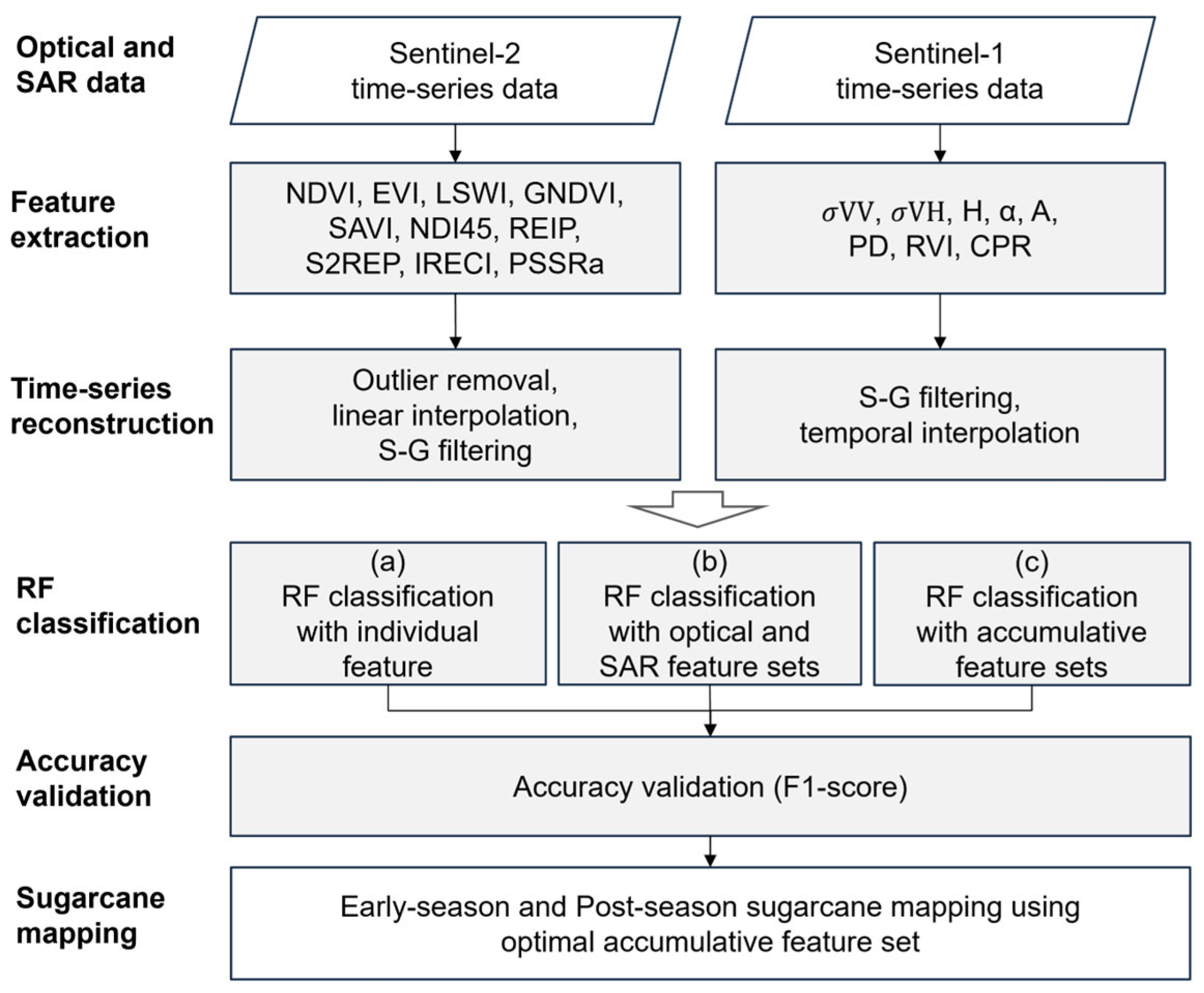
The methodological framework of this study for early-season sugarcane identification comprises four main components: (1) feature extraction from Sentinel-1 and Sentinel-2 remote sensing data, (2) time-series reconstruction to mitigate data gaps and noise, (3) sugarcane identification using random forest (RF) algorithm with various feature inputs, and (4) accuracy assessment of the identification results (Figure 3).

3.1. Feature Extraction from Sentinel-1/2 Data

Based on the Sentinel-2 multispectral imagery, 10 vegetation indices were calculated to capture crop-related biophysical and biochemical characteristics. These indices span multiple spectral domains, including visible, red-edge, near-infrared (NIR), and shortwave infrared (SWIR) regions. These indices are widely used to represent vegetation health, biomass, water stress, and chlorophyll content variations. All computations were performed on the GEE platform to enable efficient large-scale processing.

The extracted optical vegetation indices included NDVI, EVI, Land Surface Water Index (LSWI), Green Normalized Difference Index (GNDVI), Soil Adjusted Vegetation Index (SAVI), Normalized Difference Index (NDI45), Red-Edge Inflection Point Index (REIP), Sentinel-2 Red-Edge Position Index (S2REP), Inverted Red-Edge Chlorophyll Index (IRECI), and Pigment Specific Simple Ratio a (PSSRa). The selection of various indices was driven by their proven capacity to capture crop biochemical or biophysical traits across growth stages. The widely adopted NDVI provides a fundamental measure of vegetation greenness, health, and density. To address limitations in high-biomass areas and atmospheric interference, EVI offers improved sensitivity and reduced atmospheric and soil background effects. LSWI is crucial for detecting vegetation and soil moisture, enabling the monitoring of plant water stress and drought conditions [37]. GNDVI presents high sensitivity to chlorophyll concentration and photosynthetic activity, particularly in dense canopies [38]. In areas with sparse vegetation, SAVI minimizes the confounding influence of soil brightness [39]. Leveraging red-edge bands, NDI45 is highly sensitive to subtle physiological changes, aiding in the early detection of crop stress and nutrient deficiencies [40]. The position of the critical red-edge inflection point, a key indicator of chlorophyll content and phenology, is estimated by the REIP and its counterpart, S2REP [41]. IRECI demonstrates high sensitivity to elevated chlorophyll levels and effectively indicates crop stress conditions [41]. PSSRa provides a simple ratio useful for assessing photosynthetic light-use efficiency and facilitating the early detection of crop stress [42].

The equations of these vegetation indices are shown in Equations (1)–(10), where R_Blue, R_Green, R_Red, R_Nir, and R_Swir1 represent the reflectance of blue, green, red, near-infrared, and shortwave infrared bands of Sentinel-2, respectively, and R_RE1, R_RE2, and R_RE3 represent Sentinel-2 red-edge bands B5, B6, and B7, respectively.

$$\mathrm{N}\mathrm{D}\mathrm{V}\mathrm{I}={\displaystyle \frac{R_{Nir}-R_{Red}}{R_{Nir}+R_{Red}}}$$

(1)

$$\mathrm{E}\mathrm{V}\mathrm{I}={\displaystyle \frac{2.5\times \left(R_{Nir}-R_{Red}\right)}{R_{Nir}+6.0\times R_{Red}-7.5{\times R}_{Blue}+1}}$$

(2)

$$\mathrm{L}\mathrm{S}\mathrm{W}\mathrm{I}={\displaystyle \frac{R_{Nir}-R_{Swir1}}{R_{Nir}+R_{Swir1}}}$$

(3)

$$\mathrm{G}\mathrm{N}\mathrm{D}\mathrm{V}\mathrm{I}={\displaystyle \frac{R_{Nir}-R_{Green}}{R_{Nir}+R_{Green}}}$$

(4)

$$\mathrm{S}\mathrm{A}\mathrm{V}\mathrm{I}={\displaystyle \frac{\left(1+0.5\right)\times \left(R_{Nir}-R_{Red}\right)}{R_{Nir}+R_{Red}+0.5}}$$

(5)

$$\mathrm{N}\mathrm{D}\mathrm{I}45={\displaystyle \frac{R_{RE1}-R_{Red}}{R_{RE1}+R_{Red}}}$$

(6)

$$\mathrm{R}\mathrm{E}\mathrm{I}\mathrm{P}=700+{\displaystyle \frac{40\times \left(\frac{R_{Red}+R_{RE3}}{2}-R_{RE1}\right)}{R_{RE2}-R_{RE1}}}$$

(7)

$$\mathrm{S}2\mathrm{R}\mathrm{E}\mathrm{P}=705+{\displaystyle \frac{35\times \left(\frac{R_{Red}+R_{RE3}}{2}-R_{RE1}\right)}{R_{RE2}-R_{RE1}}}$$

(8)

$$\mathrm{I}\mathrm{R}\mathrm{E}\mathrm{C}\mathrm{I}={\displaystyle \frac{\left(R_{RE3}-R_{Red}\right)\times R_{RE2}}{R_{RE1}}}$$

(9)

$$\mathrm{P}\mathrm{S}\mathrm{S}\mathrm{R}\mathrm{a}={\displaystyle \frac{R_{RE3}}{R_{Red}}}$$

(10)

SAR features were extracted from Sentinel-1 polarimetric data, including the VV and VH backscatter coefficients, Cloude–Pottier decomposition parameters (H/A/α), Polarization Difference (PD), Radar Vegetation Index (RVI), and Cross-Polarization Ratio (CPR). These SAR-derived metrics exhibit unique sensitivity to vegetation structural attributes, including canopy architecture, biomass vertical distribution, surface roughness, and subsurface soil moisture dynamics.

The co-polarized backscatter coefficient (σ⁰VV) measures vertically transmitted and vertically received signals, exhibiting high sensitivity to surface characteristics including soil moisture, roughness, and bare ground conditions. Its cross-polarized counterpart (σ⁰VH), representing vertically transmitted and horizontally received signals, serves as a key indicator of vegetation structure and biomass. Polarimetric decomposition parameters offer further insights. Entropy quantifies scattering randomness, ranging from dominant single scattering (H ≈ 0, typical of bare soil) to highly random scattering (H ≈ 1, observed in dense vegetation); mean alpha angle identifies the dominant scattering mechanism, with low values indicating surface scattering, medium values volume scattering, and high values double-bounce scattering; and anisotropy characterizes the relative dominance between secondary scattering mechanisms, where A ≈ 0 suggests comparable minor mechanisms and A ≈ 1 indicates a clearly dominant secondary mechanism. Derived indices enhance vegetation monitoring. PD distinguishes scattering dominance, with low values indicating surface scattering (sparse vegetation) and high values signifying volume scattering (dense canopy). The RVI quantifies volume scattering contribution within vegetation, where higher values correspond to greater canopy density and structural complexity. Similarly, the CPR reflects depolarization intensity, with elevated values indicating denser vegetation and more complex scattering structures. The equations of PD, RVI, and CPR features are shown in Equations (11)–(13). Prior to computing RVI and CPR, the SAR backscatter values were converted from decibel (dB) to linear scale.

$$\mathrm{P}\mathrm{D}={\mathrm{\sigma }}^0\mathrm{V}\mathrm{V}-{\mathrm{\sigma }}^0\mathrm{V}\mathrm{H}$$

(11)

$$\mathrm{R}\mathrm{V}\mathrm{I}={\displaystyle \frac{4\times {\mathrm{\sigma }}^0\mathrm{V}\mathrm{H}}{{\mathrm{\sigma }}^0\mathrm{V}\mathrm{H}+{\mathrm{\sigma }}^0\mathrm{V}\mathrm{H}}}$$

(12)

$$\mathrm{C}\mathrm{P}\mathrm{R}={\displaystyle \frac{{\mathrm{\sigma }}^0\mathrm{V}\mathrm{H}}{{\mathrm{\sigma }}^0\mathrm{V}\mathrm{V}}}$$

(13)

The selection of these indices followed three primary principles, including physiological mechanisms, sensor compatibility, and feature complementarity. First, indices were prioritized based on their capacity to capture physiological status—LSWI for detecting waterlogging stress, and S2REP for monitoring chlorophyll dynamics. Second, sensor compatibility was optimized by leveraging Sentinel-2′s red-edge bands through indices like IRECI while maximizing Sentinel-1′s polarimetric signatures such as the CPR for vertical structure characterization, excluding indices requiring unavailable spectral ranges. Third, inter-index complementarity was engineered to overcome inherent limitations: optical indices fused with SAR features to mitigate biomass estimation blind spots; NDVI saturation compensated by backscatter features.

3.2. Time-Series Reconstruction for Features

Time series data of both optical and SAR features were reconstructed to improve the data quality. For the optical vegetation indices, the reconstruction process involved outlier detection and removal, temporal interpolation, and Savitzky–Golay (S-G) filtering [43].

Specifically, a threshold-based outlier removal scheme was applied. For each NDVI observation point, a sliding window of size three was used to perform linear interpolation using its preceding and subsequent valid points. Then, the observed NDVI value and the interpolated NDVI value was compared. If the absolute difference between the observed and interpolated values exceeded 0.2 (or 0.5), and the time interval to the previous observation did not exceed 20 days (or 30 days), the observation was identified as an outlier and replaced by the interpolated value. These parameters (0.2 and 0.5) were determined through systematic evaluation of multiple thresholds (0.1, 0,2 and 0.3 for 20-day interval and 0.4, 0.5, and 0.6 for 30-day interval) applied to representative samples. The reference outliers were confirmed manually through the original optical imagery and the time-series curves, and the thresholds that maximized outlier detection accuracy were used as the optimal parameters in the study area. As demonstrated by previous studies, within NDVI time-series curves, anomalous low values predominantly arise from cloud cover, variations in solar irradiance, and sensor noise—with cloud-induced anomalies exhibiting the most pronounced deviations [44,45]. Critically, clouds severely affect radiation across visible, near-infrared, and shortwave infrared spectral regions [46]. Therefore, in this study, abrupt deviations detected along the NDVI time series served as indicators of cloud-contaminated observations, guiding the filtering of other co-temporal vegetation indices.

Following the outlier correction and temporal interpolation, an S-G filter was applied to further smooth the optical time series. S-G filter has two key parameters: polynomial order and window size. Sugarcane growth curves typically exhibit a sigmoidal ‘slow-fast-slow’ pattern. A cubic polynomial optimally models this S-shaped trajectory while avoiding the oscillatory artifacts introduced by higher-order polynomials. In addition, critical growth phases such as the tillering stage persist for approximately 40–60 days. Given the 10-day temporal resolution of the provided optical vegetation index time series, a window size of 5 corresponds to a 40-day span, precisely encompassing these pivotal phenological windows. This alignment enables effective noise suppression while preserving essential growth inflection points. Therefore, in this study, the polynomial order and window size for the S-G filter were set to 3 and 5, respectively.

Similarly, the time series of SAR features were smoothed using S-G filter to suppress noise while retaining essential temporal patterns. Subsequently, temporal interpolation was conducted to harmonize the data to a consistent 10-day interval, facilitating integrated analysis with the optical datasets.

3.3. RF Classification

In this study, the RF algorithm was employed to classify sugarcane from other crop types. As an ensemble machine learning algorithm, RF constructs multiple decision trees during training and combines their outputs through majority voting or averaging to generate robust predictions. Each tree is trained on a randomly sampled subset of the training data, and at each node split, a random subset of features is considered. This strategy reduces correlation among individual trees, thereby enhancing the model’s generalization ability. RF is known for its strong robustness to noise and outliers, effectively mitigating the overfitting commonly associated with single decision trees, while maintaining high computational efficiency for large datasets. Due to its high versatility and accuracy, RF has been widely adopted in land cover classification and has shown particular effectiveness in agricultural remote sensing tasks, including crop type mapping.

In this study, a progressive temporal analysis framework was implemented, initiating sugarcane identification from the start time of growth cycle (1 March 2019) and incrementally incorporating new observations at 10-day intervals. Time-series composite feature sets with increasing temporal depth (e.g., T₁, T₁ + T₂, T₁ + T₂ + … + T_N) were generated. In addition, three experimental groups with various feature inputs were conducted to evaluate feature performances: (a) individual features derived from either optical or SAR data; (b) optical feature set, SAR feature set, and integrated optical–SAR feature set; (c) accumulative feature sets (denoted M1, M2, … M18) (Figure 4), generated according to the performances of individual features.

To reduce the impact of sampling randomness in RF algorithm, each experiment was repeated 10 times, and the average classification results across these runs were used for accuracy assessment.

3.4. Accuracy Validation

The classification accuracy of the RF model was assessed using field crop samples. A confusion matrix was constructed to evaluate classification performance, from which key metrics—producer’s accuracy (PA), user’s accuracy (UA), and the F1-score—were derived. The F1-score, defined as the harmonic mean of PA and UA, provides a balanced measure of both omission and commission errors (Equation (14)). F1-score was employed to evaluate classification effectiveness and to determine the earliest timepoint at which sugarcane could be reliably identified. The earliest identifiable timing was defined as the first temporal point at which the F1-score exceeded a threshold of 90% accuracy. To ensure statistical robustness, the mean F1-score across 10 repeated trials was reported in the results.

$$\mathrm{F}1=2\ast (\mathrm{P}\mathrm{A}\ast \mathrm{U}\mathrm{A})/(\mathrm{P}\mathrm{A}+\mathrm{U}\mathrm{A})$$

(14)

4. Results

4.1. Time Series of Features for Sugarcane and Other Crop Types

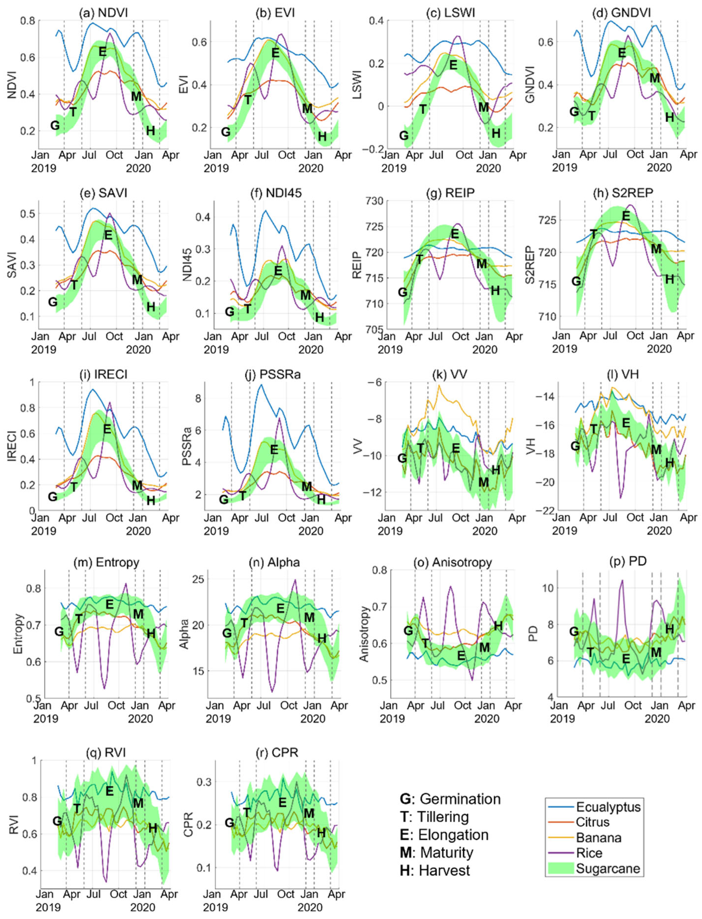
The temporal profiles of optical vegetation indices exhibited a consistent seasonal pattern characterized by an initial increase followed by a subsequent decline over the course of the sugarcane growing cycle (Figure 5a–j). Indices such as NDVI, EVI, LSWI, GNDVI, and SAVI showed synchronized phenological responses with similarly shaped curves. During the germination stage in March, all indices maintained relatively low values. This was followed by a marked increase during the tillering stage (April–May), with the maximum growth rates observed in the early elongation phase (July). Annual peak values occurred between August and October. A gradual decline began in the late elongation stage, with the steepest reductions occurring during the maturity stage, eventually returning to near-initial levels by the time of harvest.

The temporal trajectories of REIP and S2REP displayed broader waveform characteristics compared to the above indices. These red-edge-based parameters increased during early elongation (June) and sustained elevated values through October. Conversely, IRECI and PSSRa exhibited narrower temporal profiles. They followed a similar upward trend to NDVI during the vegetative growth stages, and declined at a faster rate during the later stages of the season.

The temporal profiles of SAR features are shown in Figure 5k–r. The VV and VH backscatter coefficients exhibited a pronounced increase beginning in April during the tillering stage, reaching their peak values in July during the early stem elongation phase, followed by a subsequent decline starting in August. The VV backscatter coefficient showed a steeper rate of decrease and reached its annual minimum in late December, corresponding to full canopy senescence during the maturity stage. In contrast, VH backscatter coefficient exhibited a more gradual decline, attaining its lowest values in March, which aligns with the post-season period.

The time-series patterns of entropy, anisotropy, and alpha exhibited strong inter-parameter correlations throughout the sugarcane growing season. During the tillering stage, both entropy and alpha increased rapidly and reached their peak values. These parameters then remained elevated and stable throughout the long elongation and maturity stages, before sharply declining at the onset of harvest. In contrast, anisotropy displayed an inverse trend, decreasing rapidly to its annual minimum during the tillering phase, remaining consistently low throughout the vegetative growth period, and increasing markedly during the harvest stage. These distinct temporal behaviors reflected the sensitivity of polarimetric parameters to canopy structure evolution and biomass changes during different phenological stages.

PD values were relatively high during the germination stage, indicating stronger surface scattering. As the crop developed, volume scattering increased, leading to a decline in PD. The elongation stage exhibited the lowest PD values of the year. In the maturity stage, PD values rose again, and returned to higher levels during the harvest stage. RVI and CPR showed strong mutual correlation and synchronized phenological patterns, characterized by an increasing trend during the tillering stage, sustained peak values throughout the elongation phase, followed by a gradual decline beginning at maturity, and reaching annual minima during the late harvest stage. Notably, both indices displayed large variability on each phase, suggesting substantial uncertainty in early crop identification.

4.2. Performances of Individual Optical and SAR Features

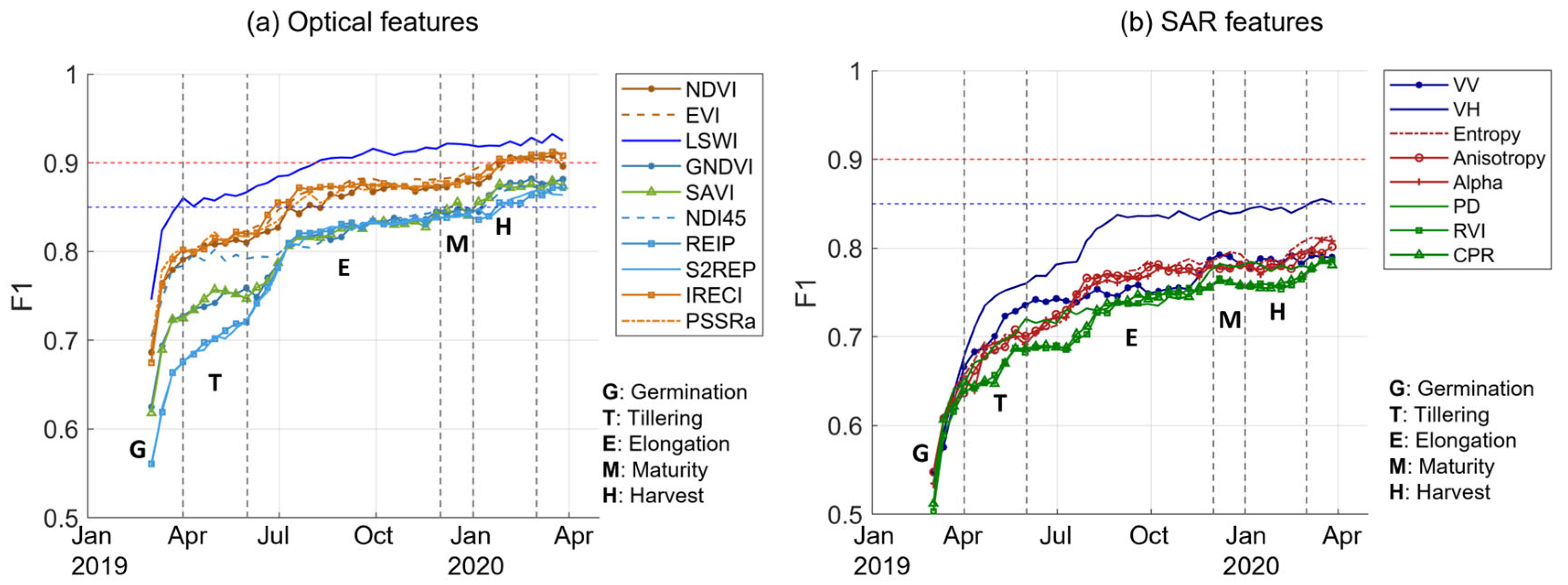
We assessed the performances of individual optical and SAR features for early-stage sugarcane identification. From the initiate stage of sugarcane growth cycle, remote sensing observations were incrementally incorporated at 10-day intervals, and identification accuracy was evaluated using the F1-score. Figure 6a,b illustrate the performance of individual optical and SAR features, respectively.

Figure 6 illustrates that with the accumulation of time-series remote sensing observations, all features demonstrated progressive improvements in early-season sugarcane identification. Among them, LSWI exhibited the strongest discriminative capability, consistently outperforming other features across all phenological stages. Its classification accuracy exceeded 85% during the tillering stage and reached 90% in the mid-elongation stage (August) during the elongation phase. In contrast, IRECI, EVI, PSSRa, and NDVI showed delayed accuracy improvements relative to LSWI. These indices followed a similar three-phase upward trend. During the tillering stage, their accuracies reached approximately 82%. As sugarcane entered the early elongation phase (June to July), accuracies improved significantly to approximately 87.5%. Accuracies continued to rise through the early-harvest period (January), eventually surpassing 90%. SAVI, GNDVI, S2REP, and REIP exhibited the weakest performance among the optical features for early-stage sugarcane identification. Their accuracies remained below 75% during tillering, improved to around 82% in the early-elongation phase, and gradually increased to a peak value lower than 85% by the end of the elongation stage. During the initial harvest phase, SAVI and GNDVI reached approximately 87.5%.

SAR features exhibited significantly weaker performance in early-season sugarcane identification compared to optical features (Figure 6b). Among SAR features, VH backscatter coefficient performed the best, maintaining relatively stable accuracy around 83.7% throughout the elongation stage. The VV backscatter coefficient ranked second during the early-elongation stage with an accuracy of approximately 75%, but was surpassed by polarimetric decomposition parameters (alpha, entropy and anisotropy) in mid-to-late elongation phases. Alpha, entropy, and anisotropy remained below 75% in early grand growth, and reached around 78% during the mid-to-late phase. PD, CPR, and RVI consistently showed the weakest performance across all growth stages, with accuracies reaching only 75% in the late-elongation stage and peaking at 77% during maturity.

These results showed that in the tillering stage, the performances of individual features were ranked as follows (from highest to lowest performance): LSWI, EVI, IRECI, PSSRa, NDVI, NDI45, VH, SAVI, GNDVI, VV, REIP, S2REP, entropy, PD, anisotropy, alpha, RVI, CPR. In the elongation stage, the performances of individual features were ranked as follows: LSWI, IRECI, EVI, PSSRa, NDVI, VH, REIP, S2REP, SAVI, GNDVI, NDI45, entropy, anisotropy, alpha, VV, CPR, RVI, PD.

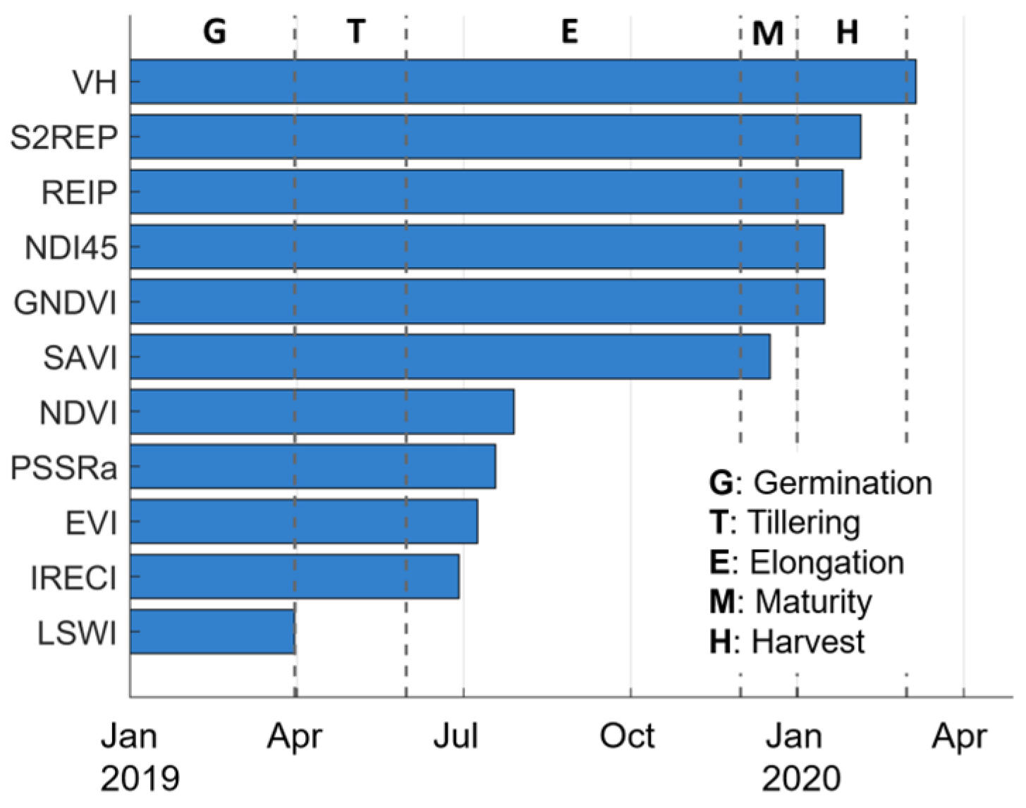
We further identified the earliest timepoints at which the F1-score reached 85% for each individual feature, as shown in Figure 7. LSWI reached this threshold as early as the germination stage. IRECI, EVI, PSSRa, and NDVI achieved 85% accuracy during the early-elongation phase (June to July), while SAVI reached this level at the maturity stage. GNDVI, NDI45, REIP, and S2REP attained 85% precision during the harvest period. The remaining features did not reach the 85% accuracy threshold at any growth stage.

4.3. Performances of Optical and SAR Feature Sets

We compared the performances of optical feature set, SAR feature set, and their combination for early-season sugarcane identification (Figure 8). The optical feature set demonstrated consistent accuracy improvements throughout the sugarcane phenological stages, achieving 85% accuracy during the initial growth stage. Performance increased further to 90% by July 20 and peaked at 92.68% on September 8—maintaining comparable accuracy (F1_max) during the post-season period. The SAR feature set demonstrated an accuracy of 80% during the early elongation stage (20 July), peaking at 83.33% in the late-elongation stage (October 18). In comparison, the combination of optical and SAR features achieved 90% accuracy by July 10 and reached a maximum F1-score of 92.98% by September 18. While this integrated approach slightly advanced the detection timeline, it did not yield higher accuracy compared to using optical features alone.

The results revealed a clear superiority of optical features over SAR features for early-season sugarcane identification, demonstrating both earlier detection and higher classification accuracy. This finding highlights the advantage of optical remote sensing, which is highly sensitive to parameters such as leaf pigment content, water content, and vegetation coverage.

4.4. Earliest Identifiable Timing Determination

Based on the accuracy assessment of individual features in Section 4.2, this part aims to search for the earliest identifiable timing for early-season sugarcane identification. A progressive feature combination strategy was implemented. Initialized with the optimal individual feature LSWI, each new feature was sequentially incorporated according to its individual performance and a series of new feature combinations (M1, M2, … M18) were generated: M1 (LSWI), M2 (M1 + IRECI), M3 (M2 + EVI), M4 (M3 + PSSRa), M5 (M4 + NDVI), M6 (M5 + VH), M7 (M6 + REIP), M8 (M7 + S2REP), M9 (M8 + SAVI), M10 (M9 + GNDVI), M11 (M10 + NDI45), M12 (M11 + entropy), M13 (M12 + anisotropy), M14 (M13 + alpha), M15 (M14 + VV), M16 (M15 + CPR), M17 (M16 + RVI), M18 (M17 + PD). Their accuracies for early-season sugarcane identification were evaluated using F1-score. Three key questions were addressed: (1) Does progressive feature accumulation accelerate the time reaching 90% accuracy threshold in early-season sugarcane identification? (2) What is the earliest possible timepoint at which ≥90% classification accuracy can be achieved? (3) What is the earliest timepoint at which accuracy reaches levels comparable to post-season accuracy (F1_max)?

To clearly demonstrate the variations in F1-score over time under different feature sets, we present the results in groups of five subfigures: (a) M1–M5, (b) M6–M10, (c) M11–M15, (d) M16–M18. As shown in Figure 9, the identification accuracies increased with the incremental temporal observations. During the tillering stage, the accuracy of these feature sets reached over 85%. The early-elongation stage (June to July) was a critical period for accuracy improvement, during which the accuracy surpassed 90% for feature sets except for M1. In the mid-elongation to late-elongation stage (August to December), accuracy reached a relatively high level and enters a plateau phase. For feature sets M1–M6, accuracies continued to increase slightly during the maturation and harvesting stages. For feature sets M7–M18, the accuracy in August could reach the levels comparable to the post-season accuracy.

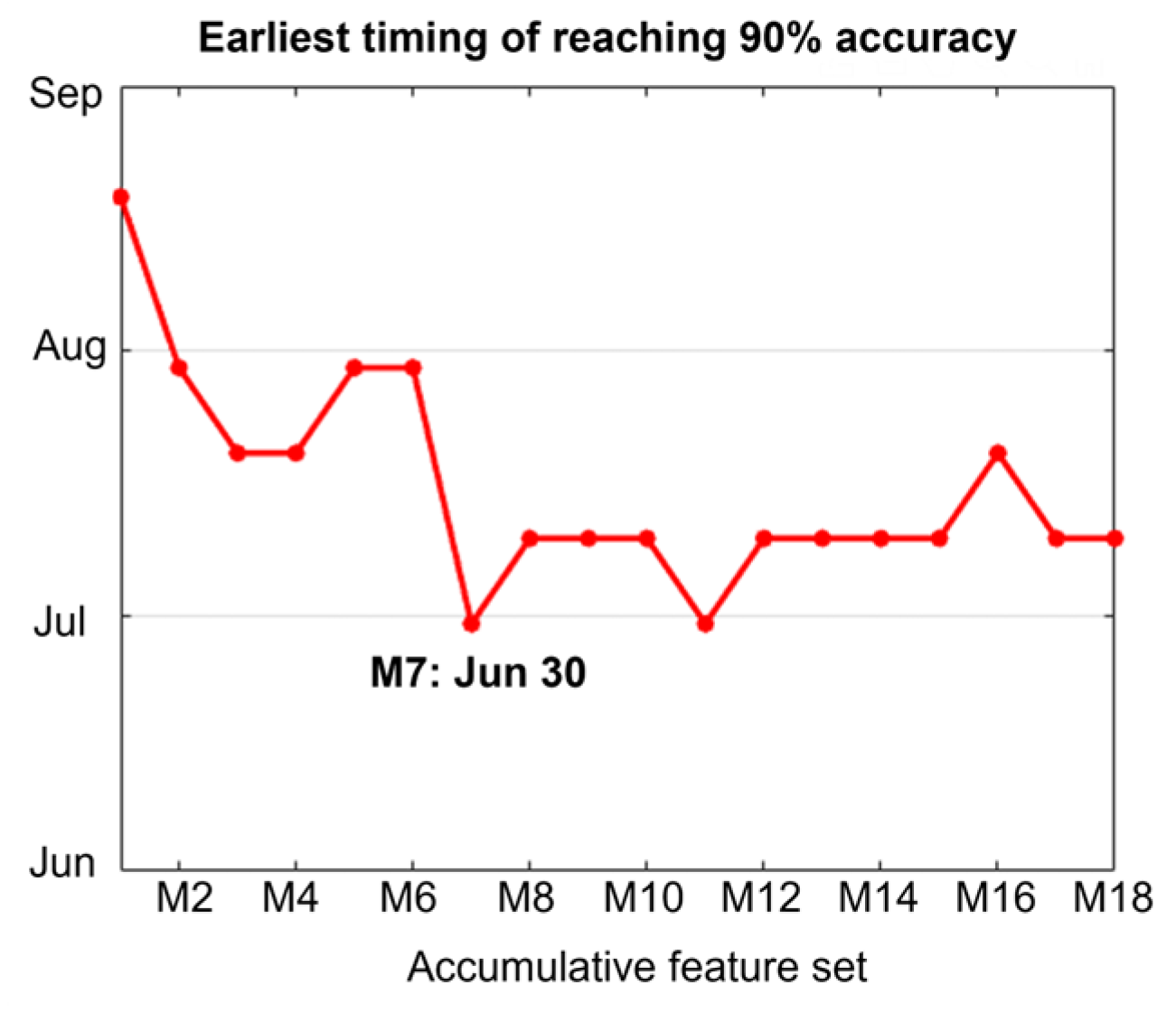
The results demonstrated that with increasing feature dimensionality when fewer than six features were utilized, sugarcane identification accuracy improved and the achievement time of 90% accuracy showed an advancing trend (Figure 10). The optimal feature set (M7), incorporating REIP along with LSWI, IRECI, EVI, PSSRa, NDVI, and VH, achieved the earliest attainment of 90% accuracy by June 30 (Figure 10), with peak performance (92.80% accuracy) reached by August 19, which was comparable to post-season accuracy. Beyond seven features, neither the maximum accuracy nor the early-achievement timing shows statistically significant improvement, indicating feature redundancy in higher-dimensional combinations. Compared to the optical feature set (Figure 8a), M7 reached 90% accuracy and the maximum accuracy more quickly.

4.5. Early-Season Sugarcane Mapping

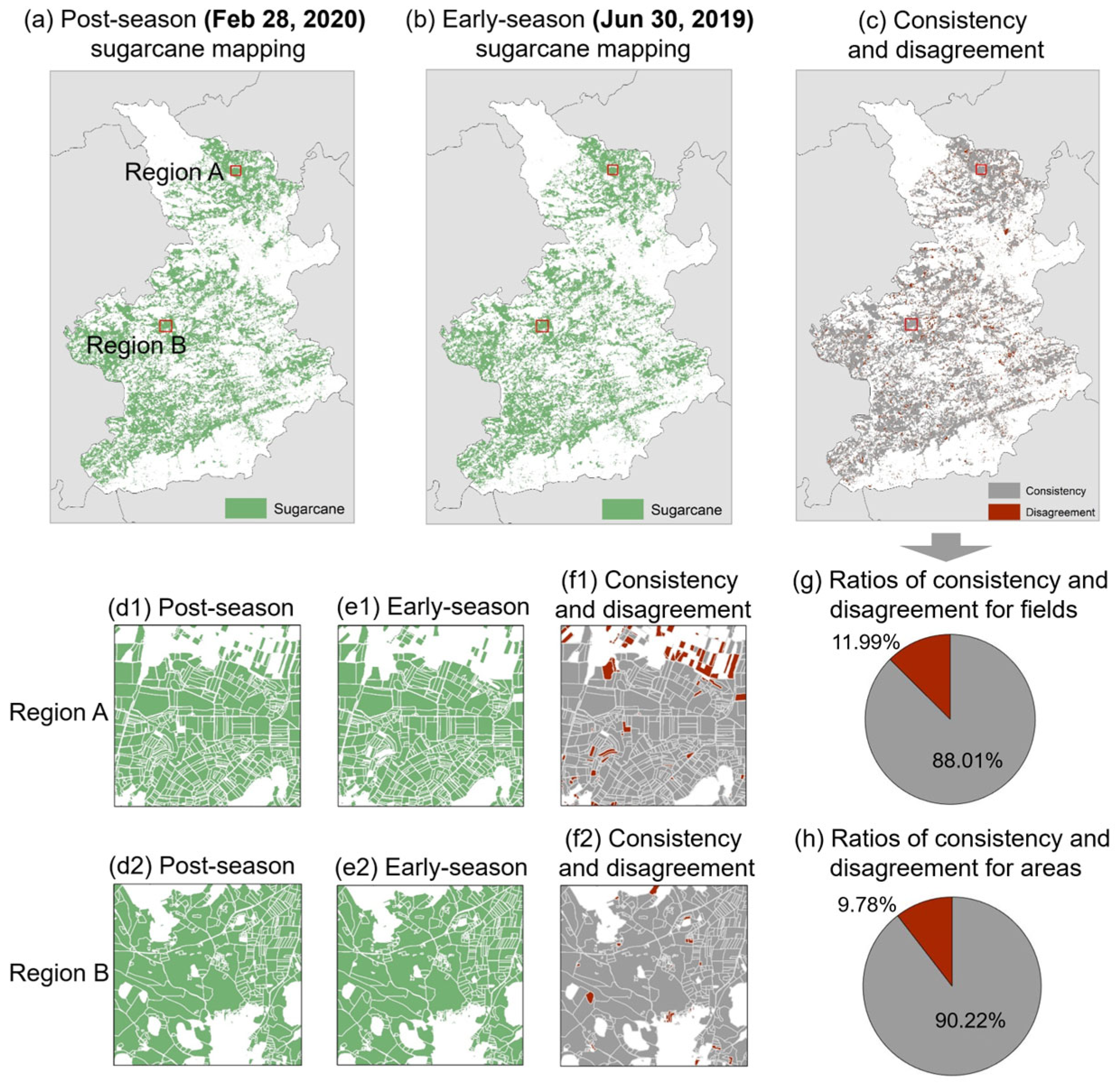
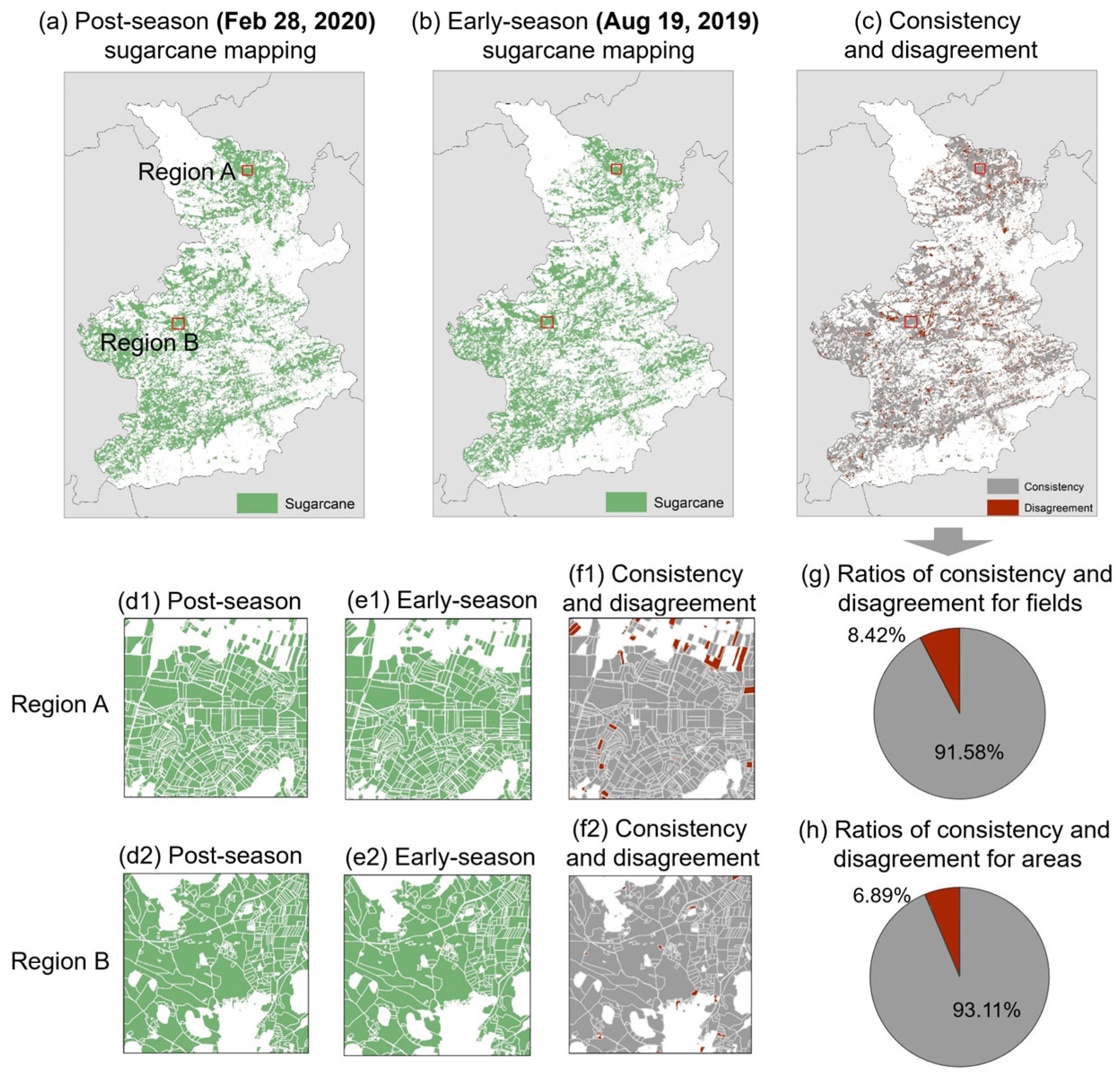
Based on the optimal feature set M7, the RF classifier was applied to conduct early-season sugarcane mapping and post-season sugarcane mapping in Fusui County. We conducted two early-season sugarcane mapping experiments, covering the periods from 1 March 2019 to 30 June 2019 and from 1 March 2019 to 19 August 2019, respectively. The post-season mapping used data from 1 March 2019 to 28 February 2020, covering the whole growth season of sugarcane. The mapping results are shown in Figure 11 and Figure 12. The early-season and post-season sugarcane mappings exhibit high similarity in the spatial distribution pattern. Furthermore, the sugarcane planting areas identified in both mapping results were compared.

For post-season sugarcane mapping, 249,421 sugarcane fields were identified, with a total planting area of 874.29 km². For early-season sugarcane mapping on 30 June, 245,703 sugarcane fields were identified in Fusui County, covering a total area of 860.47 km². For early-season sugarcane mapping on 19 August, 229,699 sugarcane fields were identified in Fusui County, covering a total area of 823.95 km².

In addition, a field-by-field comparison was conducted to assess the consistency and disagreement between the post-season mapping and the early-season mappings on 30 June and 19 August, respectively. It was found that, for the sugarcane mapping on 30 June, the number of fields with consistent and inconsistent classifications compared to the post-season mapping results were 418,947 and 57,098, respectively, accounting for 88.01% consistency and 11.99% disagreement of the total number of fields. The total area of consistent and inconsistent fields were 1319.64 km² and 143.09 km², accounting for 90.22% consistency and 9.78% disagreement of the total cultivated area (Figure 11). For the sugarcane mapping on 19 August, the number of consistent and inconsistent fields compared to the post-season mapping results were 435,955 and 40,090, respectively, accounting for 91.58% consistency and 8.42% disagreement of the total number of fields. The total area of consistent and inconsistent fields was 1361.91 km² and 100.82 km², accounting for 93.11% consistency and 6.89% disagreement of the total cultivated area (Figure 12). These results indicate that the mapping conducted on 19 August shows a higher level of consistency with the post-season mapping compared to the 30 June mapping.

5. Discussion

Previous early-season sugarcane identification studies have primarily relied on SAR backscattering coefficients (VV, VH). While effective for characterizing canopy surface roughness and moisture, these metrics exhibit limited sensitivity to biochemical parameters critical for early crop discrimination—notably chlorophyll content, nitrogen status, canopy greenness, and water stress. Our approach overcomes this limitation through synergistic integration of Sentinel-2-derived biochemical indicators spanning visible to shortwave infrared spectra and advanced polarimetric features from Sentinel-1 SLC data. Compared to conventional GRD (ground range detected) products used in prior works, the SLC data preserve the phase information, which enable Cloude–Pottier decomposition to extract the entropy, anisotropy, alpha features, probing vegetation scattering mechanisms. These complementary optical and SAR features collectively capture evolving biophysical and biochemical dynamics throughout the crop growth cycle. Through rigorous time-series analysis (Figure 6, Figure 9 and Figure 10), we identified an optimal feature combination that achieves classification accuracy comparable to post-season benchmarks as early as 6 months before harvest, which outperforms previous methods by a 3-month earlier detection margin [35].

Our systematic feature analysis revealed that LSWI, IRECI, EVI, PSSRa, NDVI, VH backscatter, and REIP demonstrated superior discriminative performance for early-season sugarcane identification. The prominence of LSWI is attributed to its sensitivity to leaf water content and soil moisture [47], which critically aligns with sugarcane’s high irrigation demands during early growth stages [13]. Red-edge parameters IRECI and PSSRa exhibited exceptional performance due to their capacity to quantify pigment concentration and crop health status. It is consistent with previous research which demonstrated the importance of red-edge bands on the early-season corn identification [4]. Similarly, the cross-polarized VH backscatter, serving as a key indicator of vegetation structure and biomass, was validated as a critical feature for early-season sugarcane identification, which has been demonstrated in previous studies [34,35]. Notably, the synergistic integration of optical and SAR features significantly accelerated early detection capabilities [4]. However, the SAR-only approach in this study achieved a maximum accuracy of 83.3%, falling short of the >90% accuracy reported in previous studies [34,35]. This performance gap likely stems from phenological similarity between sugarcane and interferential crops in the study area— particularly the banana’s and citrus’s spring canopy development, which mimics sugarcane’s radar backscatter characteristics, creating classification ambiguities.

Despite the promising performance of our optical–SAR fusion approach for early-season sugarcane identification, several limitations still exist. This study investigated the optimal feature combinations according to the rankings of individual features. However, it did not conduct a comprehensive multicollinearity assessment of selected features, which may retain highly correlated variables among the optimal feature set. Future work should implement rigorous collinearity diagnostics to eliminate redundant features. Additionally, this study did not conduct the feature importance quantification analysis. Subsequent research ought to apply feature importance evaluation to determine each feature’s contribution to classification accuracy.

Complementary to these efforts, future research should advance along four dimensions:

(1)

Optical time-series reconstruction

Persistent cloud cover and rainfall during summer monsoon months severely affected the optical data integrity in critical early-growth stages (June-July). Although abnormal observations were excluded to mitigate data quality issues, residual uncertainties persist due to insufficient valid observations during phenologically sensitive periods. Future efforts should integrate multi-sensor imputation techniques (e.g., ESTARFM (Enhanced spatial and temporal adaptive reflectance fusion model)) to reconstruct high-fidelity optical time series.

(2)

Feature set construction

While the selected vegetation indices (visible, red-edge, NIR, SWIR) provide broad spectral representation, the phenological traits of indices were underutilized. Temporal patterns in indices like NDVI and EVI show high sensitivity to crop growth progress. Future work should incorporate derivative time-series features, such as the rate of curve change and the start of growing season. In addition, this study employed commonly adopted vegetation indices and SAR parameters to establish the sugarcane mapping framework. Future research should delineate sugarcane’s biochemical and biophysical traits to develop sugarcane-specific indicators, precisely tailored to its phenological responses for enhanced early-season discriminability.

(3)

Classification algorithm selection

Although the RF classifier effectively handles high-dimensional features and demonstrates robustness against data noise, its performance remains constrained by dependency on manually engineered features. The spectral separability and subtle phenological differences among crop types during early growth stages limit the identification accuracy. Deep learning approaches, particularly convolutional-recurrent networks (e.g., CNN-LSTM), can automatically learn hierarchical spatial-spectral-temporal features from raw or minimally processed data. It helps extract subtle crop-specific cues that may be missed by traditional indices, especially under early-season phenological similarity. Unlike traditional methods that require separate preprocessing and feature engineering, deep learning supports end-to-end optimization, reducing cumulative errors. Furthermore, techniques such as dropout, data augmentation, and attention mechanisms improve robustness to noise and missing data—common in early-season imagery affected by cloud cover. (4) Generalizability testing across diverse agro-climatic zones

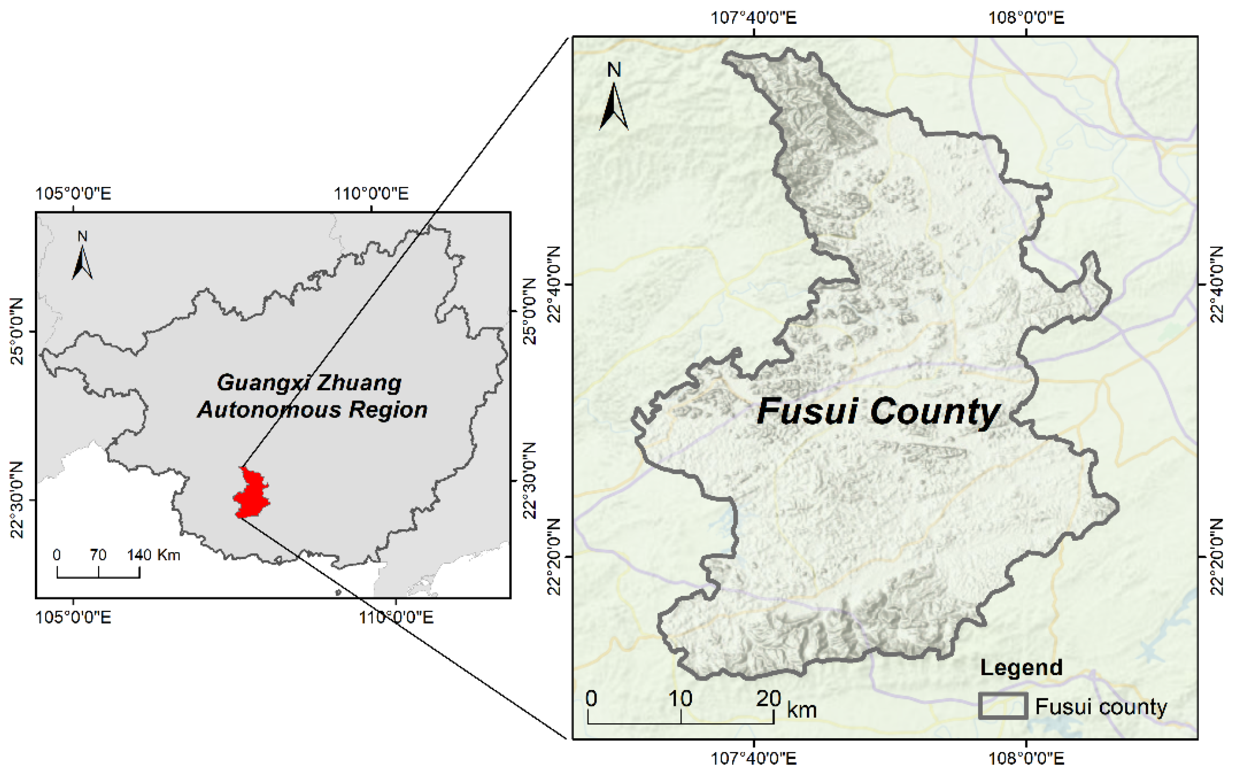
Although this study focused on Fusui County—a representative sugarcane cultivation region in South China—major production zones like Yunnan and Guangdong exhibit diversified terrain, climate, and cropping systems. Future work should validate the method’s robustness across heterogeneous agroecological zones to assess its transferability. For instance, in Yunxian County, Yunnan—a core sugarcane-producing region—the highland terrain exhibits complex topography, with steep gradients and frequent slope variations. These geographic characteristics introduce significant SAR backscatter distortion and optical spectral bias. In Zhanjiang, Guangdong, persistent cloud cover severely affects the acquisition of optical data, hindering the reconstruction of vegetation index time series. In addition, the extensive pineapple–sugarcane intercropping system in Zhanjiang creates complex spectral mixtures which are not encountered in our study area.

6. Conclusions

Early-season sugarcane identification is essential for precise field management, optimizing harvesting resource allocation, and supporting the sustainable development of the sugarcane industry. The synergistic application of optical and SAR data for early-season sugarcane identification remains unexplored in previous studies. This study aims to determine whether the integration of optical and SAR data improves identification accuracy or accelerates the time to achieve reliable identification and what is the most efficient feature combination for early detection.

The results showed that among all features, LSWI demonstrated the best early identification capability. Based on the performance of individual features, this study incrementally added features and evaluated the performances of accumulative feature sets. It was found that the seven-dimensional feature combination (LSWI, IRECI, EVI, PSSRa, NDVI, VH backscatter coefficient, and REIP) achieved two critical milestones: reaching initial 90% accuracy by 30 June (early-elongation stage) and peak performance matching post-season level (92.80% accuracy) by 19 August (mid-elongation stage), which are an eight-month and a six-month advancement lead over post-season identification, respectively. Finally, this study performed early-season (30 June and 19 August, respectively) and post-season sugarcane mapping based on the feature combination for Fusui County. It is indicated that the early-season mapping on 19 August has high similarity with the post-season mapping.

This study establishes a robust multi-sensor framework for early-season sugarcane identification, demonstrating that synergistic integration of optical and SAR data enables crop mapping with accuracy comparable to post-season mapping as early as six months prior to harvest. This advancement could provide information for timely and precision agronomic management during critical growth stages.