Remote Sensing Interpretation of Geological Elements via a Synergistic Neural Framework with Multi-Source Data and Prior Knowledge

Abstract

Geological elements are fundamental components of the Earth’s ecosystem, and accurately identifying their spatial distribution is essential for analyzing environmental processes, guiding land-use planning, and promoting sustainable development. Remote sensing technologies, combined with artificial intelligence algorithms, offer new opportunities for the efficient interpretation of geological features. However, in areas with dense vegetation coverage, the information directly extracted from single-source optical imagery is limited, thereby constraining interpretation accuracy. Supplementary inputs such as synthetic aperture radar (SAR), topographic features, and texture information—collectively referred to as sensitive features and prior knowledge—can improve interpretation, but their effectiveness varies significantly across time and space. This variability often leads to inconsistent performance in general-purpose models, thus limiting their practical applicability. To address these challenges, we construct a geological element interpretation dataset for Northwest China by incorporating multi-source data, including Sentinel-1 SAR imagery, Sentinel-2 multispectral imagery, sensitive features (such as the digital elevation model (DEM), texture features based on the gray-level co-occurrence matrix (GLCM), geological maps (GMs), and the normalized difference vegetation index (NDVI)), as well as prior knowledge (such as base geological maps). Using five mainstream deep learning models, we systematically evaluate the performance improvement brought by various sensitive features and prior knowledge in remote sensing-based geological interpretation. To handle disparities in spatial resolution, temporal acquisition, and noise characteristics across sensors, we further develop a multi-source complement-driven network (MCDNet) that integrates an improved feature rectification module (IFRM) and an attention-enhanced fusion module (AFM) to achieve effective cross-modal alignment and noise suppression. Experimental results demonstrate that the integration of multi-source sensitive features and prior knowledge leads to a 2.32–6.69% improvement in mIoU for geological elements interpretation, with base geological maps and topographic features contributing most significantly to accuracy gains.

1. Introduction

Geological elements serve as foundational components in ecological environments, land use, and spatial planning decisions. Accurate interpretation of their spatial information is critical for evaluating ecosystem services, managing land resources, and advancing environmental protection efforts [1,2]. Traditional geological mapping methods, which rely heavily on field surveys and manual visual interpretation, suffer from high labor costs, low efficiency, and limited spatial coverage, making them inadequate for the demands of large-scale remote sensing data processing and rapid mapping [3,4]. The integration of remote sensing and artificial intelligence offers a new technical pathway for the automated and fine-scale interpretation of geological elements. Geological element interpretation based on remote sensing and intelligent algorithms targets thematic geological mapping by leveraging data sources such as optical imagery, radar data, and geological surveys. It draws upon geological knowledge and expert interpretation experience while employing machine learning and deep learning algorithms to achieve high-precision identification of surface elements such as lithology and soil types [5].

However, each remote sensing modality has its inherent limitations. Optical imagery provides rich spectral information but is highly susceptible to interference from cloud cover and vegetation, limiting its effectiveness in complex surface environments [6,7]. Synthetic aperture radar (SAR) imagery offers all-weather acquisition capabilities and good surface penetration, but its spatial resolution is typically lower than that of optical imagery, making it less effective at capturing fine-scale geological boundaries and texture features [8,9]. Moreover, SAR data is significantly affected by speckle noise. To compensate for the information gaps among different modalities, researchers—drawing inspiration from human visual interpretation—have introduced sensitive features such as elevation, slope, and texture statistics, along with prior geological knowledge such as base geological maps (GMs) and stratigraphic boundaries, to provide structured semantic constraints for neural networks, particularly in areas with weak spectral separability [10]. However, both sensitive features and prior knowledge exhibit pronounced spatiotemporal heterogeneity, meaning their contributions to interpretation performance vary across geomorphic regions. For instance, in Karst plateau areas with significant surface relief, DEM and slope information markedly enhance the recognition of Karst distributions [11]. On the other hand, coarse mapping scales, outdated geological data, and inconsistencies with current surface conditions can cause misalignment between knowledge representation and remote sensing inputs, potentially leading to erroneous guidance [12]. This regional adaptability issue results in inconsistent enhancement effects in general models, hindering the development of universally effective strategies. Consequently, there is an urgent need to select and match the most discriminative sensitive features and prior knowledge types based on specific geomorphic and geological backgrounds, enabling precise guidance and adaptive enhancement.

At the same time, multi-source remote sensing data fusion continues to face several structural challenges [13,14,15]. Fundamental differences exist in the sensing mechanisms of different data sources, such as spectral reflectance, microwave backscattering, and topographic geometric attributes [16,17]. These modalities also differ significantly in terms of spatial resolution, temporal acquisition cycles, viewing angles, and noise characteristics [18]. In the absence of a unified feature representation and an effective mechanism for mutual complementation, multimodal fusion is prone to semantic mismatches, feature redundancy accumulation, and even information conflicts [19]. These issues can hinder model convergence, degrade generalization performance, and lead to negative transfer. For example, during the fusion of SAR and optical imagery, failure to properly handle view-angle discrepancies and noise disturbances may cause the model to overfit low-quality features from one modality, thereby exacerbating boundary ambiguity and class confusion [20]. Therefore, it is imperative to develop an intelligent interpretation framework with capabilities for cross-modal alignment, feature complementarity, and adaptive fusion, enabling accurate extraction and robust generalization of geological elements.

In this work, we conduct a systematic evaluation of how multimodal sensitive features and prior knowledge improve the accuracy of geological element interpretation using remote sensing data. Specifically, we select a representative arid to semi-arid region in Northwest China as the study area, characterized by complex lithological structures, significant terrain relief, and sparse vegetation cover. In this region, we construct a geological interpretation dataset incorporating five types of sensitive features and one type of prior knowledge. Using several mainstream deep learning models, we assess the performance improvements contributed by different combinations of these auxiliary inputs. Furthermore, we propose a semantic segmentation network for geological elements, named MCDNet, which consists of two specialized modules: a improved feature rectification module (IFRM) and an attention-enhanced fusion module (AFM). The IFRM performs mutual correction of cross-modal features in both channel and spatial dimensions, while the AFM enhances multimodal feature fusion through information exchange and cross-attention mechanisms. Together, these modules address the challenges of cross-modal feature misalignment and noise interference commonly encountered in multimodal data fusion. At a glance, we deliver the following contributions:

• We construct a geological element interpretation dataset that integrates Sentinel-1 SAR imagery, Sentinel-2 multispectral imagery, the digital elevation model (DEM), texture features, normalized difference vegetation index (NDVI), and GMs, incorporating both sensitive features and prior geological knowledge.
• We systematically evaluate the improvement effects of various sensitive features and prior knowledge on remote sensing-based geological interpretation using five representative deep learning architectures.
• We propose MCDNet, which integrates an IFRM and an AFM to achieve effective cross-modal feature alignment and enhancement through a combination of calibration and attention mechanisms.

2. Related Work

In recent years, the development of remote sensing technologies and intelligent algorithms has provided efficient tools for geological element interpretation [21,22,23,24]. Traditional manual interpretation methods, which heavily rely on expert knowledge and costly field surveys, face serious limitations in large-scale and high-frequency mapping scenarios. In contrast, machine learning techniques are capable of learning hierarchical feature representations and exhibit strong classification performance and generalization ability, making them widely applied in geological information extraction and lithological identification tasks [25]. Manap et al. [26] constructed a multi-source dataset combining ASTER optical imagery, Sentinel-1 SAR, and DEM in western Antalya, Turkey. They systematically evaluated the performance of four classification algorithms—MLC, RF, SVM, and NN—under different data fusion schemes. Their results showed that SVM achieved the highest accuracy when integrated data were used. Zhang et al. [27] proposed a machine learning classification framework centered on SVM and RF based on two open well-logging datasets, Teapot Dome and FORCE 2020. They established a standardized pipeline for data preprocessing and feature engineering, improving both lithological classification accuracy and regional generalization. Pereira et al. [28] addressed the insufficiency of 1:50,000-scale lithological mapping in the Beiras region of Portugal by integrating multi-temporal Landsat-8 imagery, field hyperspectral measurements, and X-ray fluorescence geochemical characteristics of rock samples. Using the J48 decision tree algorithm, they achieved the accurate classification of major lithological units, demonstrating the feasibility and scalability of fusing multi-source remote sensing and geochemical data. Kumar et al. [29] tackled the complex classification of carbonaceous and non-coal banded strata in the Talcher coalfield, India. They applied a range of supervised learning algorithms—including SVM, decision tree, RF, MLP, and XGBoost—based on well-logging data such as gamma-ray, density, and resistivity curves, enabling the effective differentiation of multiple lithological types. Despite their effectiveness on small samples and low-dimensional features, traditional machine learning models still rely on handcrafted features or shallow representations. This limits their ability to automatically capture complex nonlinear spatial structures and semantic information from raw high-dimensional data. The challenge becomes even more pronounced in multi-source remote sensing fusion scenarios, where spectral, geometric, temporal, and resolution heterogeneities exist across modalities, making it difficult for conventional machine learning approaches to model and represent them in a unified and synergistic manner.

Deep learning has demonstrated significant advantages in the intelligent interpretation of geological elements from remote sensing data due to its end-to-end feature learning capability [30,31,32]. Unlike traditional machine learning methods that rely on handcrafted features, deep learning can automatically extract complex nonlinear structures and multi-scale semantic information from remote sensing imagery, making it particularly well-suited for areas with rugged topography and complex terrain [33]. Shirmard et al. [34] combined convolutional neural networks with traditional classifiers such as SVM and MLP to perform lithological mapping in a mineral-enriched region of Southeastern Iran using multi-source imagery from Landsat-8, ASTER, and Sentinel-2. Their results showed that the CNN–ASTER combination achieved the highest classification accuracy. Han et al. [35] proposed AMSDFNet, an adaptive multi-source data fusion network based on Landsat-8 and Sentinel-2 imagery, which enabled the high-precision joint interpretation of multiple geological elements including lithology, soil, water bodies, and glaciers. Lu et al. [36] introduced distance fields of geological interpretation markers and topographic-sensitive features as explicit structural knowledge into the IAFFNet network, improving soil type classification accuracy. He et al. [37] developed a context-enhanced multi-scale feature fusion network that, when combined with the SimAM attention mechanism, significantly improved the segmentation accuracy of lithology and water bodies in Landsat-8 imagery. Li et al. [38] proposed a shared deep representation model that integrates geological traverse labels with remote sensing features to support multi-class geological mapping at the 1:25,000 and 1:50,000 scales, achieving accurate object recognition and spatial consistency. Dong et al. [39] fused Gaofen-5 hyperspectral and Sentinel-2B multispectral imagery within the ViT-DGCN architecture. By enhancing spatial–spectral features via SFIM fusion and incorporating Transformer and dynamic graph convolution modules, their model achieved high interpretation accuracy using only 1% of training samples. Ouyang et al. [40] addressed the challenge of lithological classification in densely vegetated regions of the middle Yangtze River by proposing LSBPNet, a network that incorporates prototype-driven geological prior knowledge for the precise segmentation of engineering lithology. Despite these advances, there remains a lack of systematic and quantitative analysis on how sensitive features and prior knowledge contribute to performance enhancement. This gap limits our understanding of the relative contributions of different features under varying geomorphic conditions, lithological configurations, or sensor modalities. Moreover, most deep learning models focus primarily on feature fusion strategies while neglecting the semantic shift and structural mismatch caused by differences in spatiotemporal resolution across modalities, which often leads to feature redundancy, modal bias, or even negative transfer during the fusion process.

3. Research Area and Dataset

3.1. Study Area Overview

The study area is located in the typical arid to semi-arid geomorphic belt of northwestern China and is strongly influenced by the topography and climatic patterns associated with the Tianshan Mountains [41]. This region exhibits a characteristic composite landform consisting of alpine zones and intermontane basins [42]. The Tianshan Mountains extend in a north–south direction through the center of the study area, dividing it into two distinct geomorphic units: the northern intermontane basins and the southern canyon–plateau system. The northern slope features relatively gentle terrain, with well-developed alluvial fans and broad valley plains that are favorable for sedimentary rock distribution and vegetation growth. In contrast, the southern slope is characterized by rugged topography, including steep ridges, deeply incised valleys, and glacial development zones, forming a typical high-mountain geomorphological landscape. Geologically, the region is situated at the western margin of the Tianshan orogenic belt and exposes stratigraphic sequences spanning from the Paleozoic to the Cenozoic. It hosts a wide variety of lithologies, including metamorphic, igneous, and sedimentary rocks. Common rock types include coarse sandstone, sandstone, conglomerate, granite, gneiss, phyllite, gabbro, andesite, and carbonate rocks. The lithological diversity and complex associations provide a solid foundation for remote sensing-based lithological interpretation. Furthermore, multiple rounds of geological mapping and thematic surveys have been conducted in this area, yielding a wealth of GM and prior knowledge data. The region is well-covered by remote sensing imagery, with evenly distributed geological units and clearly defined interpretation boundaries, making it an ideal test site for developing intelligent interpretation methods of geological elements.

3.2. Dataset for the Study Area

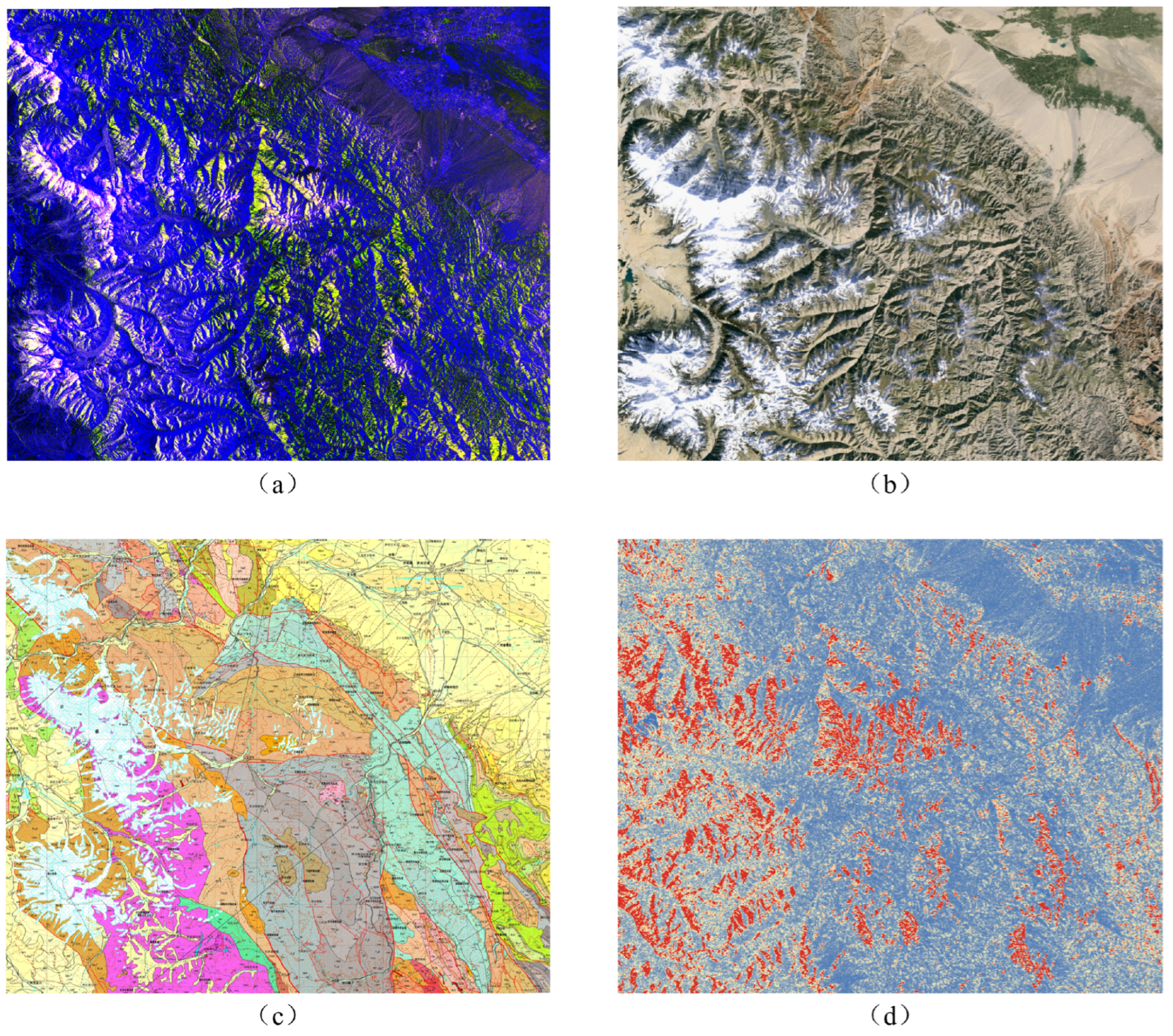
The SAR data used in this study are acquired from the Sentinel-1 satellite system, part of the Copernicus program operated by the European space agency. Equipped with a C-band SAR sensor, Sentinel-1 provides all-weather, day-and-night imaging capabilities, making it especially suitable for surface observations under complex geomorphological and climatic conditions. Sentinel-1 supports multiple imaging modes, including interferometric wide (IW) swath, extra wide swath, stripmap, and wave mode. Among them, the IW mode offers a balance between high spatial resolution (approximately 2.7–3.5 m × 22 m) and wide-area coverage, making it the primary acquisition mode for land surface remote sensing applications. In addition, Sentinel-1 supports various polarization configurations, including single polarization and dual polarization. Dual polarization provides enhanced sensitivity to surface structure, roughness, and moisture content, thereby improving the discrimination of geological units and related features. In this study, dual-polarized Level-1 Ground Range Detected products acquired in IW mode are selected as input data. This configuration combines strong backscattering capability with geometric stability, contributing to improved accuracy in geological interpretation as shown in Figure 1a.

The optical remote sensing data used in this study are obtained from the Sentinel-2 satellite, part of the Copernicus Earth Observation Program operated by the ESA. Sentinel-2 provides 13 spectral bands covering the visible to shortwave infrared regions. In this study, three atmospheric correction bands with lower spatial resolution (60 m)—Band 1, Band 9, and Band 10—are excluded. The remaining 10 bands, which have strong surface discrimination capability, are selected as input data. Among them, the bands with a native resolution of 20 m are resampled to 10 m using bilinear interpolation to achieve uniform spatial resolution and enhance the recognition of fine-scale object boundaries. The selected bands include the visible bands (Bands 2–4), which are useful for distinguishing vegetation and soil cover; the red-edge bands (Bands 5–7), which are sensitive to chlorophyll content and subtle vegetation stress, thus aiding in indirect lithological mapping; the near-infrared bands (Bands 8), which are effective in detecting vegetation structure and surface moisture variation; and the shortwave infrared bands (Bands 11 and 12), which are critical for differentiating minerals and rock types due to their spectral sensitivity to hydroxyl-bearing and ferrous minerals. These bands offer excellent spectral sensitivity for geological applications, enabling the identification of surface features such as vegetation, bare land, water bodies, minerals, and soil moisture as shown in Figure 1b.

The prior knowledge used in this study consists of a 1:250,000-scale geological base map compiled by the Basic Geological Survey Center of the Henan Geological Survey between 2003 and 2005 through extensive field investigations. The map is currently published and publicly accessible via the Geoscientific Data & Discovery Publishing System as shown in Figure 1c. This GM provides detailed spatial patterns of geological units within the study area, including information on geological ages, stratigraphic units, lithological assemblages, structural boundaries, and fault systems. It features high spatial and temporal resolution and strong regional representativeness, serving as a valuable source of expert prior knowledge for geological interpretation.

DEM, slope, and NDVI imagery were obtained via the Google Earth Engine platform. Topography plays a key role in soil formation processes by influencing the redistribution of moisture, heat, and parent materials. Therefore, DEM data are introduced in this study as a quantitative representation of terrain to support soil-related geological interpretation. The DEM is sourced from the shuttle radar topography mission (SRTM), while slope data are derived from the DEM. NDVI is calculated from Sentinel-2 imagery using standard band combinations.

SAR data have a natural advantage in capturing surface roughness and structural variation. Different geological elements exhibit distinct texture patterns in SAR imagery, which are essentially reflected in the spatial gray-level distribution and statistical relationships of image pixels. In this study, texture features are extracted using the classical gray level co-occurrence matrix (GLCM) method. Five representative statistical features are computed: angular second moment, dissimilarity, contrast, homogeneity, and correlation. These features respectively describe energy distribution, local gray-level variation, edge strength, texture uniformity, and spatial correlation. To improve directional robustness, GLCMs are computed at four orientations (0°, 45°, 90°, and 135°), and the average value across these directions is used as the final texture feature representation as shown in Figure 1d.

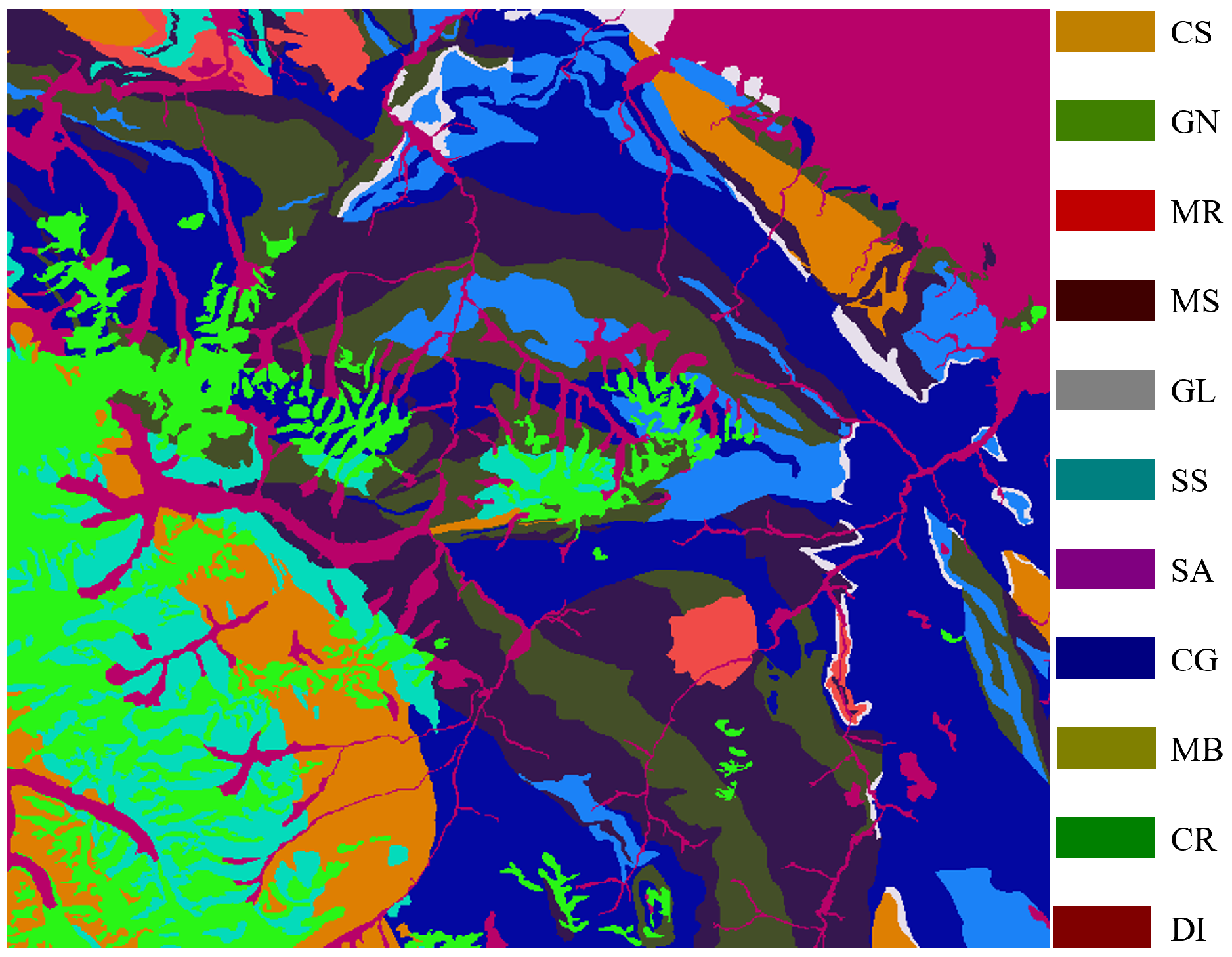
The label dataset was generated by domain experts from the Xining Center for Integrated Natural Resource Surveys, China Geological Survey, through multiple rounds of geological mapping and field investigations. Four field survey routes were included in the manual validation process, which confirmed that the overall accuracy of the manual interpretation reached 91.6%. This result meets the current national standards for remote sensing geological surveys in China, which require interpretation accuracy above 80% in exposed areas, indicating that the dataset is highly reliable as shown in Figure 2. The major geological elements in the study area are categorized into 11 classes: coarse sand (CS), granite (GN), metamorphic rock (MR), mudstone (MS), glacier (GL), siltstone (SS), sandstone (SA), conglomerate (CG), marble (MB), carbonate rock (CR), and diorite (DI). The proportion of each class within the training and test datasets is summarized in

Table 1. Proportion of each geological class in the train and test datasets. The categories include coarse sand (CS), granite (GN), metamorphic rock (MR), mudstone (MS), glacier (GL), siltstone (SS), sandstone (SA), conglomerate (CG), marble (MB), carbonate rock (CR), and diorite (DI).

Geological Element	Train Dataset (%)	Test Dataset (%)
CS	25.44	25.10
GN	6.99	6.94
MR	8.05	7.49
MS	5.92	7.11
GL	12.97	11.60
SS	14.48	14.27
SA	7.68	8.44
CG	3.78	4.40
MB	0.78	0.41
CR	11.60	12.05
DI	2.32	2.20

. After clipping and preprocessing, a total of 1287 image patches of size 224 × 224 pixels were generated from the multi-source data, each with a spatial resolution of 10 m.

4. Proposed Method

To overcome the limitations of single-source remote sensing data—such as incomplete information and limited penetration capability—in geological element interpretation, and to further enhance the guiding role of sensitive features and prior knowledge in the intelligent interpretation process, we propose a MCDNet. The network is designed to enable the collaborative fusion of optical imagery, SAR, sensitive features, and geological prior knowledge. Specifically, MCDNet incorporates two core modules, the IFRM and the AFM, as shown in Figure 3. Under a dual-branch architecture, these modules are responsible for extracting, co-modeling, and structurally fusing features from different modalities. This design effectively suppresses spatiotemporal inconsistencies and noise interference across modalities. During the fusion stage, a multi-level feature coupling decoder is introduced to hierarchically integrate multi-scale fused features, combining spatial and semantic information. This enables the network to produce high-precision interpretation results.

4.1. Framework Overview

The backbone of the dual-branch MCDNet adopts a parallel ResNet-50 architecture, where each branch is designed to extract discriminative features from different modalities, such as multispectral imagery, SAR data, sensitive features, and prior knowledge. Each branch independently models modality-specific feature representations, while a cross-modal information interaction mechanism enables dynamic correction between hierarchical feature layers, improving the complementarity and robustness of the learned features. The IFRM is designed to use information from one modality to guide and refine the feature representation of the other, thereby mitigating inconsistencies caused by inherent noise across modalities. Embedded at each stage of the backbone, IFRM performs mirror-like interactions between the outputs of the two branches, dynamically adjusting their structural representations to improve semantic consistency and spatial alignment. To further improve the expressive power of multimodal fusion, the AFM processes the refined dual-modal features through information exchange and structural integration. It first conducts deep feature interaction via a self-attention-driven symmetrical dual-channel structure, followed by a $1\times 1$ convolution for channel-wise feature fusion. The output is then fed into the decoder. Inspired by the UPerNet architecture, we adopt a multi-level feature coupling decoder that progressively integrates fused features from different stages of the backbone. This hierarchical embedding strategy improves high-level semantic representation while preserving low-level spatial details, thereby enhancing the final interpretation results in terms of both spatial resolution and semantic consistency.

4.2. Improved Feature Rectification Module

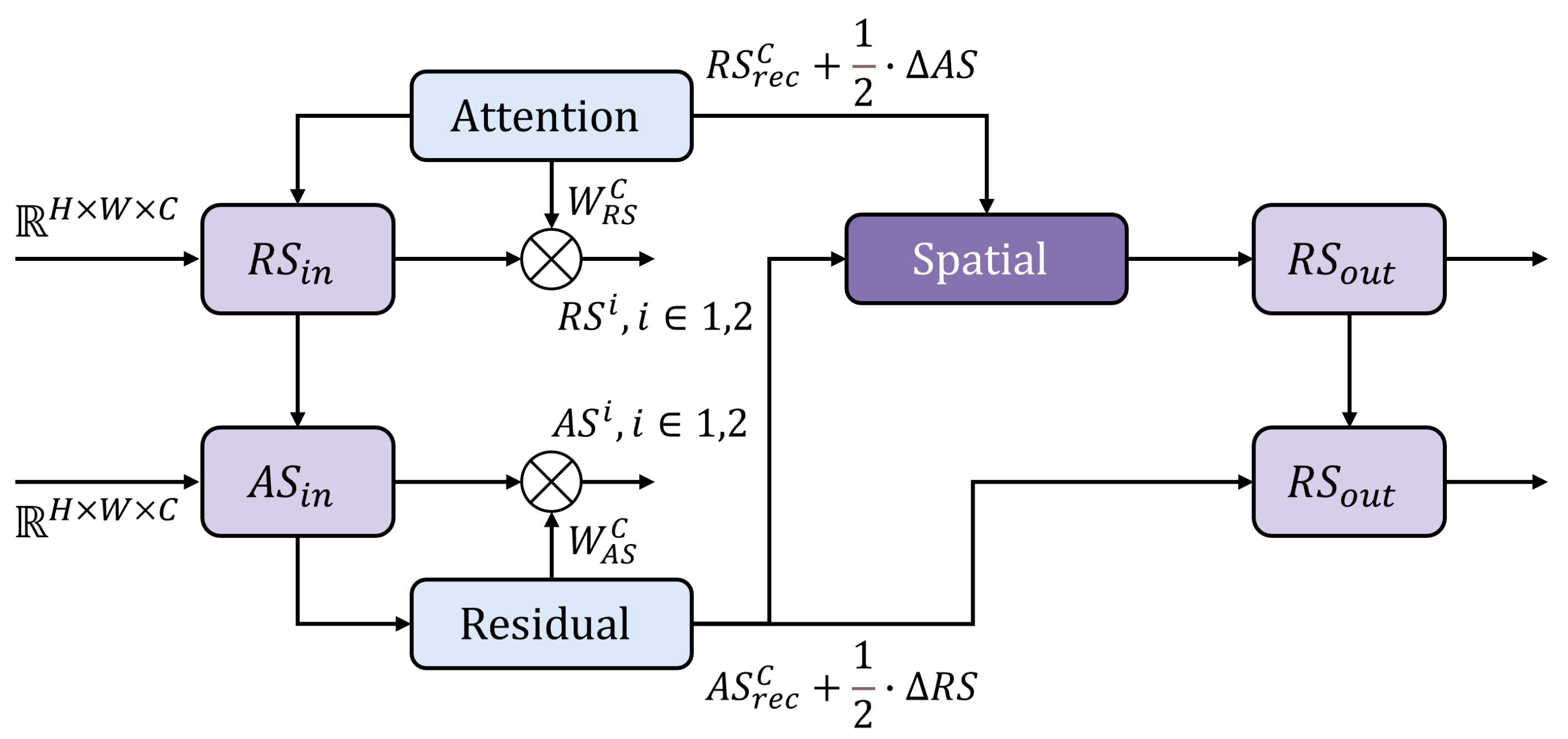
To enhance semantic coordination across different modalities in multi-source remote sensing data fusion, we propose an IFRM as shown in Figure 4. Based on joint channel–spatial calibration of heterogeneous features, the module incorporates a cross-channel attention gating mechanism and a residual spatial adaptation pathway. This design effectively alleviates inter-modal feature interference and improves structural consistency in deep feature representations.

The input features from the dual-branch ResNet-50 backbone, corresponding to the multispectral remote sensing modality and the auxiliary features, are denoted as ${RS}_{in}\in {\mathbb{R}}^{H\times W\times C}$ and ${AS}_{in}\in {\mathbb{R}}^{H\times W\times C}$, where H, W, and C represent the spatial dimensions and the number of channels, respectively. These two features are projected from the spatial domain into two attention vectors, $W_{RS}^C\in R^C$ and $W_{AS}^C\in R^C$. To capture the importance of each channel, both input features are processed through global average pooling and global max pooling along the channel dimension, producing four one-dimensional descriptor vectors. These vectors are then concatenated to form a unified channel descriptor vector $Y\in R^{4C}$. Subsequently, a multi-layer perceptron followed by a sigmoid activation function is applied to Y to generate the attention weights for the two modalities, denoted as $W_{RS}^C$ and $W_{AS}^C$:

$$W_{RS}^C,W_{AS}^C=F_{split}\left(\sigma \left(F_{mlp}\left(Y\right)\right)\right),$$

(1)

where $F_{mlp}(·)$ denotes a multi-layer perceptron, $\sigma (·)$ is the sigmoid activation function, and $F_{split}(·)$ represents the operation that splits the output vector into two modality-specific weight vectors. These channel-wise attention weights are then used to recalibrate the input features, resulting in the refined features $R{S}_{rec}^C$ and $A{S}_{rec}^C$, which are computed as

$$R{S}_{rec}^C=W_{AS}^C\otimes A{S}_{in},$$

(2)

$$A{S}_{rec}^C=W_{RS}^C\otimes R{S}_{in},$$

(3)

where ⊗ denotes channel-wise matrix multiplication.

To improve the adaptability of the correction process to nonlinear inter-modal differences, we introduce a residual guidance mechanism. A $1\times 1$ convolutional residual projection network ${\phi }_{proj}(·)$ is constructed to generate structural residual signals for each modality:

$$\Delta RS=R{S}_{in}-{\phi }_{\mathrm{proj}}\left(R{S}_{in}\right),$$

(4)

$$\Delta AS=A{S}_{in}-{\phi }_{\mathrm{proj}}\left(A{S}_{in}\right),$$

(5)

These residual signals are then integrated into the recalibrated features as modulation terms to enhance the representation capability with respect to inter-modal differences:

$$R{S}_{rec}=R{S}_{rec}^C+{\displaystyle \frac{1}{2}}·\Delta AS,$$

(6)

$$A{S}_{rec}=A{S}_{rec}^C+{\displaystyle \frac{1}{2}}·\Delta RS,$$

(7)

While the channel-wise correction focuses on learning global attention weights to perform global feature alignment, a spatial perspective correction is introduced in the feature refinement module (FRM) to further account for local inconsistencies. The two input features $R{S}_{in}$ and $A{S}_{in}$ are concatenated and mapped through two spatial weight masks $W_{RS}^S\in R^{H\times W}$ and $W_{AS}^S\in R^{H\times W}$. The spatial embedding is implemented using two $1\times 1$ convolutional layers with a ReLU activation function. Then, a sigmoid function is applied to obtain a spatial embedding tensor $F^S\in R^{H\times W\times 2}$, which is split into the spatial attention weights for the two modalities:

$$F^S={Conv}_{1\times 1}\left(ReLU\left({Conv}_{1\times 1}\left(R{S}_{in}\parallel A{S}_{in}\right)\right)\right),$$

(8)

$$W_{RS}^S,W_{AS}^S=f_{split}\left(\sigma \left(F^S\right)\right),$$

(9)

Following a strategy similar to the channel-wise correction, spatial-wise correction is applied to both feature branches. Finally, the outputs of channel and spatial corrections are aggregated to obtain the overall corrected features:

$$R{S}_{out}=R{S}_{in}+{\displaystyle \frac{1}{2}}\left(R{S}_{rec}^C+R{S}_{rec}^S\right),$$

(10)

$$A{S}_{out}=A{S}_{in}+{\displaystyle \frac{1}{2}}\left(A{S}_{rec}^C+A{S}_{rec}^S\right),$$

(11)

4.3. Attention-Enhanced Fusion Module

To further enhance the interactive representation capability of multi-source modality fusion features, we introduce the AFM. Based on the structure of IFRM, AFM is designed as a two-stage architecture consisting of information re-encoding and deep fusion, which explicitly reinforces inter-modal information complementarity and semantic alignment. In the information exchange stage, a symmetric dual-branch structure is retained. A multi-head cross-attention mechanism is applied to perform global information interaction between the two branches. In the feature fusion stage, a mixed channel embedding is used to project the concatenated features back to the original input dimension.

First, the input features $R{S}_{in},A{S}_{in}\in R^{H\times W\times C}$ are reshaped into matrices of size $R^{N\times C}$, where $N=H\times W$. The reshaped features are denoted as $R{S}_f,A{S}_f\in R^{N\times C}$. Then, a linear transformation is applied to generate interaction and residual vectors for semantic alignment:

$$X_{RS}^{inter},X_{RS}^{res}=\phi \left(R{S}_f\right),$$

(12)

$$X_{AS}^{inter},X_{AS}^{res}=\phi \left(A{S}_f\right),$$

(13)

where $\phi (·)$ denotes a shared MLP structure.

A multi-head cross-attention mechanism is then introduced to compute the Query, Key, and Value vectors for each modality. The interaction vectors are embedded into the Keys and Values of each attention head, with dimensions $R^{N\times C_{head}}$. Cross-attention matrices $\widehat{RS},\widehat{AS}$ are obtained by computing the attention between the interaction vectors, context vectors, and the opposite branch features. This enables a shift from point-to-point semantic mapping to global context-driven interaction, addressing the limitations of AFM, which operates at the feature-map level.

To fuse the enhanced dual-modal features and improve their structural consistency in spatial representation, we introduce a joint aggregation structure guided by deep convolution. The two enhanced feature maps are first concatenated and projected back to the original channel dimension, i.e., $concat(\widehat{RS},\widehat{AS})\in R^{H\times W\times 2C}$. Then, a simple $1\times 1$ convolution is applied to fuse the dual-branch features. Finally, a depthwise convolution layer ${DWConv}_{3\times 3}$, combined with a skip-connection structure, is employed to further capture local contextual associations and enhance the robustness of the segmentation output.

4.4. Multi-Level Feature Coupling Decoder

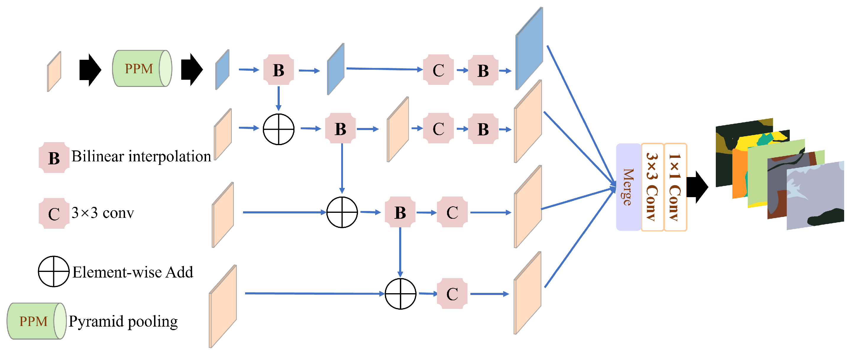
To fully integrate spatial and semantic information from different levels and enhance the model’s ability to perceive geological boundaries and fine-grained structures, this study employs a multi-level feature coupling decoder as shown in Figure 5. This decoder is constructed based on multi-scale feature representation and includes two sub-modules: the pyramid pooling module (PPM) and the feature pyramid network (FPN), which are responsible for capturing contextual and cross-scale inter-level information, respectively. The final interpretation prediction is achieved through cascaded fusion.

To improve the model’s understanding of the overall image structure, the PPM is used to capture contextual information at different scales. Acting on the deepest feature map from the backbone, the PPM performs adaptive average pooling with four different strides (stride = 1, 2, 3, 6). Each pooled feature is passed through a $1\times 1$ convolution to reduce dimensionality and then upsampled back to the original spatial resolution using bilinear interpolation. The multi-scale features are concatenated with the original feature along the channel dimension and fused to generate enhanced context-aware representations.

To further integrate features from different levels, the FPN is utilized to progressively align and fuse multi-scale features $F_0,F_1,F_2,F_3$ from the encoder. Processing proceeds from deep to shallow layers. For each level $i\in \{3,2,1\}$, the higher-level feature $F_i$ is upsampled to match the spatial resolution of $F_{i-1}$ and added residually:

$$F_{i-1}^{\prime }=F_{i-1}+Bi(F_i,F_{i-1}),$$

(14)

where $Bi(a,b)$ denotes the bilinear interpolation of a to the size of b.

Subsequently, all levels of features are passed through a $3\times 3$ convolution to reduce redundancy and are upsampled to match the resolution of the shallowest feature $F_0$. Finally, the four processed feature maps $F_0,F_1^{″},F_2^{″},F_3^{″}$ are concatenated along the channel dimension and fused through cascaded convolution for final inference:

$$F_i^{″}=Bi({Conv}_{3\times 3}\left(F_i^{\prime }\right),F_0),$$

(15)

$$F_{out}={Conv}_{1\times 1}\left({Conv}_{3\times 3}\left(Concat(F_0,F_1^{″},F_2^{″},F_3^{″})\right)\right),$$

(16)

5. Experiments and Analysis

5.1. Experimental Setting

In this work, we utilize a variety of remote sensing data sources, including multispectral imagery, SAR imagery, DEM, slope, texture features, NDVI, and GM. The dataset is randomly divided into training, validation, and test sets with a ratio of 6:2:2. To comprehensively evaluate the enhancement effects of sensitive features and prior knowledge on intelligent remote sensing interpretation, we construct six input configurations based on different modality combinations: (1) MS, which fuses multispectral imagery and SAR imagery; (2) MGM, which combines MS with GM; (3) MDE, which combines MS with DEM; (4) MTS, which integrates MS with slope; (5) MGL, which adds GLCM-based texture features extracted from SAR to MS; and (6) MNV, which integrates MS with the NDVI.

To validate the effectiveness of MCDNet, we compare it with several mainstream deep learning segmentation models. These include classical semantic segmentation networks such as fully convolutional networks (FCNs, using ResNet-101 as the backbone) [43] and UPerNet (based on ResNet-50) [44], as well as advanced Transformer-based architectures including SegFormer [45], Vision Transformer (ViT) [46], and BEiT [47]. All experiments are conducted on a desktop with 64 GB RAM and an NVIDIA RTX 3090 GPU. The hyperparameters are set as follows: a batch size of 8, a learning rate of $1\times {10}^{-4}$, the Adam optimizer, and a total of 500 training epochs. To ensure the robustness of results, each experiment is repeated multiple times, and the average performance is reported.

5.2. Evaluation Metrics

To objectively evaluate the performance of the experiments, we adopt two widely used metrics in semantic segmentation: overall Pixel Accuracy (oPA) and mean Intersection over Union (mIoU).

The oPA metric measures the proportion of correctly classified pixels to the total number of pixels, and is defined as

$$oPA={\displaystyle \frac{{\sum }_{i=1}^{N}T{P}_i}{{\sum }_{i=1}^N(T{P}_i+F{P}_i+F{N}_i)}},$$

(17)

where $T{P}_i$ denotes the number of true positive pixels for class i, $F{P}_i$ denotes the number of false positives, and $F{N}_i$ represents the number of false negatives. N is the total number of classes.

The mIoU metric calculates the average ratio between the intersection and the union of the predicted and ground truth areas for each class:

$$mIoU={\displaystyle \frac{1}{N}}\sum _{i=1}^N{\displaystyle \frac{T{P}_i}{T{P}_i+F{P}_i+F{N}_i}}.$$

(18)

5.3. Ablation Experiments

To systematically evaluate the actual contributions of MCDNet’s modular design and the guidance mechanisms of sensitive features and prior knowledge to the intelligent remote sensing interpretation of geological elements, we conduct two types of ablation studies. The first focuses on structural ablation analysis of the individual components within MCDNet, while the second investigates the performance gains from incorporating sensitive features and prior knowledge. Specifically, we use UPerNet (ResNet-50) as the baseline model and progressively integrate the proposed modules and various types of sensitive features and domain knowledge. A comparative analysis is performed to assess the influence of each configuration on overall accuracy. All experiments are repeated multiple times under identical parameter settings, and the average results are reported to ensure evaluation stability.

5.3.1. Ablation Study on the MCDNet Modules

The ablation study on the MCDNet modules is summarized in

Table 2. Module ablation experiments of MCDNet.

Method	MS	IFRM	AFM	oPA (%)	mIoU (%)
UPerNet (ResNet-50)	✓	–	–	67.2 ± 0.5	38.0 ± 0.4
MCDNet	✓	✓	–	71.6 ± 0.4	42.1 ± 0.3
	✓	–	✓	70.8 ± 0.6	41.5 ± 0.4
	✓	✓	✓	72.0 ± 0.3	43.6 ± 0.2

. In the baseline model, which fuses multispectral and SAR imagery using UPerNet, the oPA and mIoU reach 67.2% and 38.0%, respectively. After incorporating the IFRM module, the oPA and mIoU increase by 4.4% and 4.1%, respectively. This improvement is attributed to the dual-perspective correction mechanism in the channel and spatial dimensions, where cross-channel gated attention and residual spatial adaptation paths help alleviate interference between heterogeneous modalities and enhance the coordination of feature modeling. Further, by integrating the AFM module, the oPA and mIoU improve by 3.6% and 3.5%, respectively. This gain results from the use of a multi-head cross-attention mechanism, which establishes a more effective alignment path between the MS and SAR modalities. It addresses the issues of information redundancy and misalignment in the original fusion process, enabling the model to better focus on fine-grained differences, particularly around geological boundaries. When both IFRM and AFM modules are incorporated simultaneously, the oPA and mIoU reach 72.0% and 43.6%, corresponding to improvements of 4.8% in oPA and 5.6% in mIoU compared to the baseline model. These results indicate that the combined use of the two modules significantly enhances the model’s ability to perceive and interpret complex geological semantics in multi-source data.

5.3.2. Ablation Study on Sensitive Features and Prior Knowledge

To evaluate the effectiveness of sensitive features and prior knowledge in enhancing remote sensing-based geological interpretation, an ablation study is conducted on five types of auxiliary data sources, GM, DEM, slope, GLCM, and NDVI, as shown in

Table 3. Ablation experiments on sensitive features and prior knowledge enhancement.

Method	MS	GM	DEM	Slope	GLCM	NDVI	oPA (%)	mIoU (%)
UPerNet (ResNet-50)	✓						67.2 ± 0.5	38.0 ± 0.4
	✓	✓					70.4 ± 0.3	41.5 ± 0.5
	✓		✓				68.2 ± 0.4	39.6 ± 0.3
	✓			✓			69.6 ± 0.6	40.3 ± 0.2
	✓				✓		70.3 ± 0.3	40.8 ± 0.4
	✓					✓	69.4 ± 0.4	39.2 ± 0.5
MCDNet	✓						72.0 ± 0.4	43.6 ± 0.2
	✓	✓					76.1 ± 0.3	48.2 ± 0.3
	✓		✓				75.8 ± 0.5	47.0 ± 0.4
	✓			✓			75.6 ± 0.4	47.5 ± 0.2
	✓				✓		76.2 ± 0.3	46.8 ± 0.5
	✓					✓	75.1 ± 0.6	45.9 ± 0.4

. Each feature is individually added to the multi-source dataset MS and tested under both the baseline UPerNet and the proposed MCDNet architecture. The results demonstrate that incorporating sensitive features and prior knowledge significantly improves interpretation accuracy across both models. For the UPerNet baseline, oPA is increased by 1.0–3.2%, and mIoU improved by 1.2–3.5%. In contrast, our MCDNet achieves even greater performance gains, with oPA increasing by 3.1–4.2% and mIoU by 2.3–4.6%. Notably, the integration of GM results in the highest mIoU (48.2%) and the second-optimal oPA (76.1%) under the MCDNet framework. This outcome highlights the semantic alignment between stratigraphic and lithological patterns embedded in GM and the target geological elements, which provides explicit classification boundaries for feature learning. The optimal oPA (76.2%) is obtained by incorporating GLCM features derived from SAR imagery, indicating that texture statistics are particularly effective for reinforcing global classification signals, especially in regions with sharp boundary transitions and texture discontinuities. In contrast, the NDVI contributes the least to model performance improvement, likely due to the sparse vegetation coverage in arid and semi-arid regions, where vegetation has limited influence on lithogenesis and thus provides minimal discriminative information. These results confirm that MCDNet exhibits superior capability in leveraging sensitive features and prior knowledge. Nonetheless, the selection of such features should be carefully aligned with the environmental context and geological formation mechanisms to optimize interpretability and generalization in remote sensing-based geological analysis.

5.4. Comparison Experiments

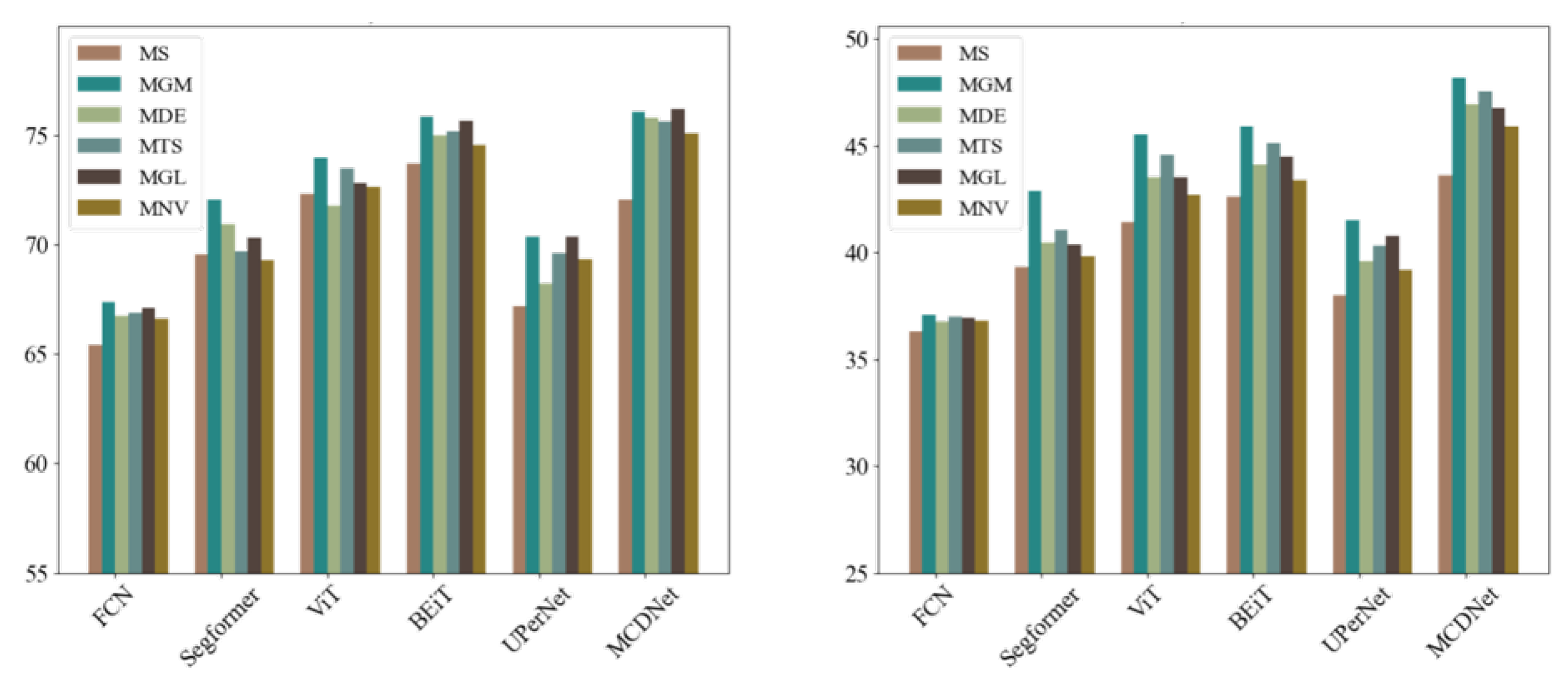
This study compares the performance of MCDNet with several mainstream semantic segmentation models in the task of intelligent geological element interpretation using remote sensing data. Furthermore, it evaluates the practical contributions of various sensitive features and prior knowledge in supporting the interpretation process. Figure 6 presents the oPA and mIoU achieved by different models under six input scenarios. From the overall trend, all sensitive features and prior knowledge—except for the NDVI—provide varying degrees of positive performance gain, demonstrating the effectiveness of integrating remote sensing data with prior geological knowledge for intelligent interpretation. MCDNet consistently achieves the optimal results across all scenarios, highlighting its superior capability in heterogeneous data fusion and feature discrimination. In contrast, traditional models such as FCN and SegFormer show relatively weaker performance, particularly when only MS imagery is used as input, with mIoU values generally falling below 40%. This indicates limitations in their ability to model fused information. Transformer-based models such as ViT and BEiT achieve second-optimal results, with noticeable improvements upon the integration of prior knowledge. This suggests that while these models are effective in high-dimensional data representation and feature modeling, they still lag behind MCDNet in terms of fusion efficiency and stability.

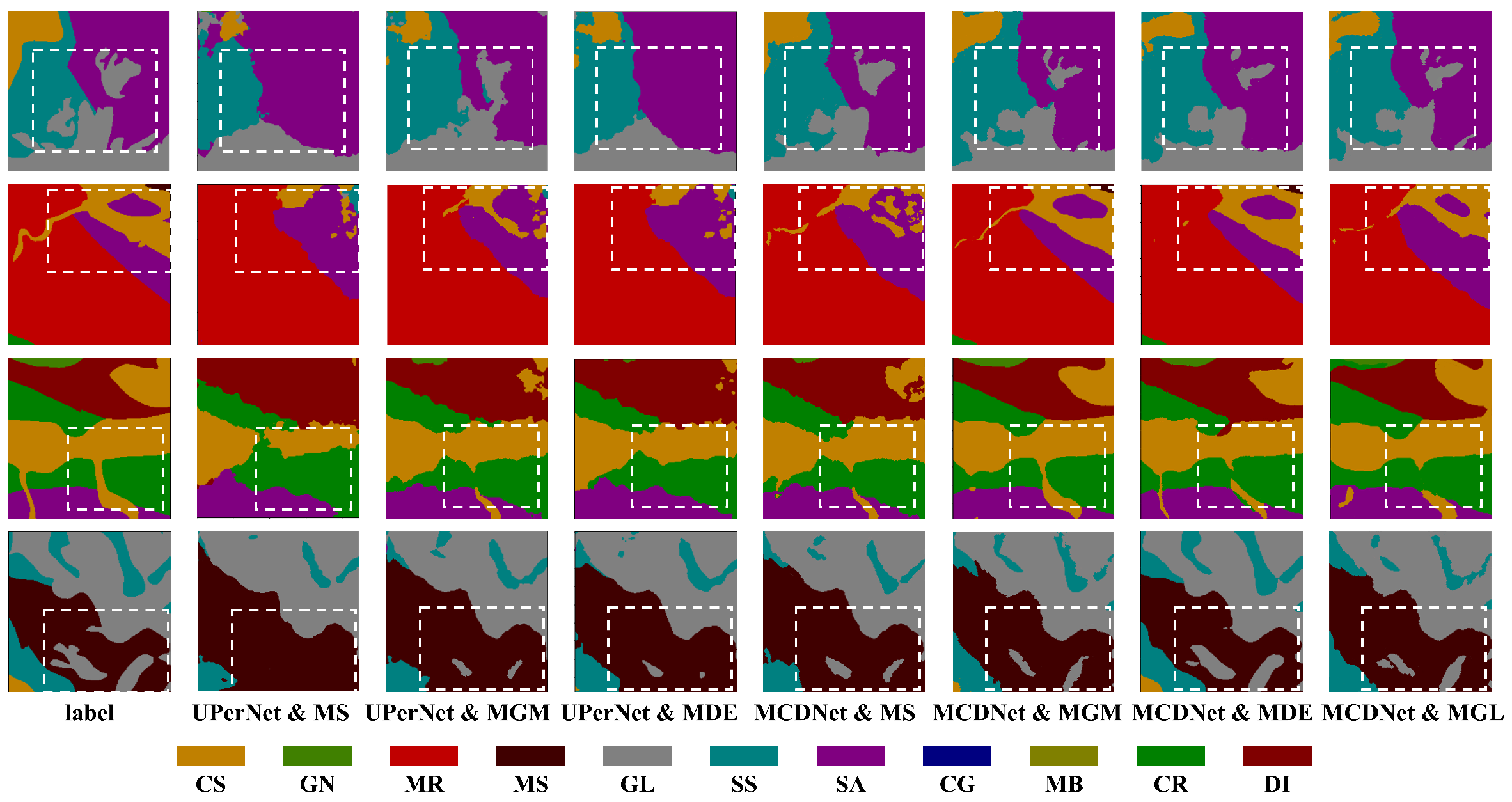
Figure 7 presents a visual comparison between the baseline model UPerNet and the proposed MCDNet under four representative conditions guided by sensitive features and prior knowledge: MS, MGM, MDE, and MGL. It is noteworthy that the MTS scenario is not included due to its high spatial similarity with DEM, resulting in limited discriminative effects. Similarly, the NDVI case is excluded from visualization as the sparse vegetation cover in the study area contributes minimally to geological interpretation. Overall, MCDNet exhibits clearer boundary delineation and more accurate category discrimination across various regions, with particularly enhanced performance in complex zones (highlighted by white dashed boxes). Under the guidance of GM and DEM, MCDNet demonstrates superior recognition of lithological classes with ambiguous boundaries or similar textures, such as MR and CR, significantly reducing class confusion. These visual results strongly confirm the advantages of MCDNet in discriminative power and robustness through multi-source data fusion and sensitive feature guidance. In particular, the model shows improved generalization capability in geologically complex regions and areas lacking dense prior knowledge, outperforming the baseline method.

Under the MS dataset input condition, significant performance differences are observed among the models in geological element interpretation as summarized in

Table 4. Comparison of models on MS dataset using PA and IoU (%).

Metrics	Method	CS	GN	MR	MS	GL	SS	SA	CG	MB	CR	DI
PA	FCN	77.7	54.7	51.5	40.7	78.7	67.9	43.0	54.0	14.7	59.5	25.1
	UPerNet	77.8	53.8	57.1	40.2	84.3	64.0	42.3	56.6	28.4	58.0	38.8
	Segformer	80.7	59.3	58.5	39.7	85.5	67.2	41.5	53.3	17.4	59.7	47.7
	ViT	82.9	61.8	56.4	36.2	88.8	65.7	41.3	52.7	47.2	60.3	55.2
	BEiT	85.1	61.2	59.7	40.5	89.1	63.1	46.2	56.8	48.4	57.2	56.3
	MCDNet	80.7	63.9	61.0	43.8	88.0	70.8	47.1	63.0	45.5	60.9	48.7
IoU	FCN	68.8	31.6	38.0	28.2	64.4	45.2	30.4	37.2	6.2	41.2	9.2
	UPerNet	68.9	30.5	42.3	28.0	73.0	41.0	29.8	39.6	10.8	39.1	15.2
	Segformer	72.5	35.7	43.7	27.8	74.7	43.9	29.1	34.5	7.0	41.3	20.2
	ViT	75.3	38.2	41.8	24.9	79.7	42.6	29.1	35.6	20.8	41.9	25.9
	BEiT	78.1	37.1	45.0	28.2	80.5	40.4	33.3	39.9	21.5	38.5	26.7
	MCDNet	72.4	40.5	46.2	31.1	78.4	48.3	34.2	45.9	19.4	42.6	20.9

. Among all compared models, MCDNet achieves the overall optimal performance, obtaining the highest pixel accuracy (PA) and intersection over union (IoU) in 7 out of 11 geological categories. For example, in the CG, MCDNet reaches a PA of 63.0%, outperforming the second-optimal BEiT by 6.2% in PA and 6.0% in IoU. This result demonstrates MCDNet’s robustness and superior representational capability when dealing with small-sample and boundary-ambiguous classes. Notably, GR—the most abundant class in the training dataset—achieves second-optimal segmentation performance, suggesting that class frequency alone does not guarantee optimal results. Conversely, GL, which constitutes only 13% of the training data, still attains the highest accuracy. This highlights that high interpretation performance relies more on the model’s capacity to distinguish subtle geological differences and effectively model cross-modal interactions than merely on data distribution.

Under the MGM input condition, the experimental results are summarized in

Table 5. Comparison of models on MGM dataset using PA and IoU (%).

Metrics	Method	CS	GN	MR	MS	GL	SS	SA	CG	MB	CR	DI
PA	FCN	79.8	58.5	53.4	37.2	82.2	68.4	39.6	56.1	20.5	55.5	27.7
	UPerNet	82.2	58.7	55.6	39.2	86.0	66.5	42.0	58.4	53.8	57.1	54.5
	Segformer	80.9	61.3	58.6	43.3	89.0	68.6	43.2	60.5	53.1	56.1	53.9
	ViT	83.1	63.0	58.3	43.4	89.9	65.4	48.6	61.3	59.3	63.7	61.7
	BEiT	85.6	64.9	59.9	44.3	90.5	69.4	48.7	58.8	54.3	62.3	61.0
	MCDNet	85.7	66.9	62.7	47.3	89.5	72.6	51.3	64.4	59.8	65.0	59.0
IoU	FCN	71.3	35.4	38.4	25.4	69.7	46.1	27.5	39.2	8.0	37.0	10.2
	UPerNet	74.5	35.4	40.6	27.1	75.3	43.3	29.7	41.5	25.9	38.9	24.5
	Segformer	72.7	37.3	43.9	30.7	80.4	45.6	30.5	43.6	24.8	38.1	24.2
	ViT	75.7	39.5	43.3	30.9	81.7	42.3	35.4	43.9	30.6	45.3	32.3
	BEiT	78.9	41.6	45.4	31.6	82.6	46.6	35.4	41.7	26.1	44.1	30.8
	MCDNet	79.0	44.2	48.1	34.5	80.8	50.4	38.1	47.2	31.6	47.0	29.4

. MCDNet achieves the highest PA and IoU in 9 out of 11 geological categories. Notable improvements are observed in small-sample or low-texture classes such as CG, GN, and MR. For example, MCDNet achieves a PA of 64.4% for CG, representing a 5.6% improvement in PA and a 5.5% improvement in IoU over BEiT. This demonstrates that high-level semantic information contained in geological maps—such as stratigraphic age and tectonic unit boundaries—provides clear prior constraints for the accurate classification of weak categories. Moreover, classes with limited sample representation in the training set, such as MB and CR, also show improved recognition performance, with PA values of 59.8% and 65.0%, respectively. These correspond to accuracy gains of 39.3% and 9.5% over FCN, effectively mitigating the bias toward dominant classes. These findings confirm the comprehensive advantages of MCDNet in handling sparse samples, modeling inter-class similarity, and leveraging high-level semantic features for improved geological element interpretation.

Under the MDE dataset input condition, the experimental results presented in

Table 6. Comparison of models on MDE dataset using PA and IoU (%).

Metrics	Method	CS	GN	MR	MS	GL	SS	SA	CG	MB	CR	DI
PA	FCN	80.9	59.9	51.5	37.9	78.7	66.9	38.3	57.0	17.3	59.0	25.3
	UPerNet	78.8	58.8	51.1	35.0	85.6	65.4	42.9	55.3	41.8	59.4	56.6
	Segformer	80.5	59.3	50.7	41.3	88.3	68.7	43.2	54.6	44.5	57.6	49.5
	ViT	81.9	62.6	59.4	43.6	88.0	63.4	47.0	58.9	55.8	50.5	56.5
	BEiT	86.4	59.7	59.3	43.9	89.0	69.0	45.3	59.6	49.4	57.2	60.4
	MCDNet	85.1	64.2	61.7	45.9	89.6	73.2	51.3	64.2	54.8	65.0	55.8
IoU	FCN	72.7	36.5	36.9	26.1	64.8	43.7	26.6	40.4	7.1	40.5	9.1
	UPerNet	70.2	35.7	36.4	23.7	74.5	42.5	30.4	38.2	16.8	40.9	26.2
	Segformer	72.3	35.6	36.3	28.8	79.0	46.1	30.7	37.7	18.8	38.8	21.2
	ViT	74.0	49.3	44.6	31.1	78.5	39.9	34.2	41.8	27.3	42.1	26.4
	BEiT	80.0	36.2	44.9	31.2	79.9	46.8	32.5	42.1	22.6	38.9	30.6
	MCDNet	78.3	41.1	47.2	32.8	81.0	51.7	37.9	47.1	26.7	46.5	26.5

show overall performance improvements across all models compared to the baseline multi-source input. These improvements are particularly evident in categories with pronounced terrain variation and strong topographic dependence in their geological distribution. MCDNet achieves the highest PA and IoU in 8 out of the 11 geological categories. Notably, categories such as GN, CG, and MR—which are more sensitive to terrain changes—demonstrate substantial accuracy gains. For example, in the GN category, MCDNet achieves a PA of 64.2%, outperforming ViT by 1.6%, and an IoU of 41.1%, exceeding BEiT by 4.9%. It is also worth mentioning that although GL has a relatively low sample proportion, it consistently achieves the highest PA across all models, with MCDNet reaching 89.6%. This suggests that GL exhibits distinct terrain-related characteristics that are effectively captured through DEM-enhanced features, facilitating its accurate identification by the model. DEM is especially effective in mountainous and glaciated terrains where elevation and slope sharply constrain lithological distribution, such as in alpine sedimentary sequences and faulted metamorphic belts. The elevation gradient contributes to stratigraphic layering visibility and supports geomorphological boundary delineation.

Under the MTS dataset input condition, the experimental results (

Table 7. Comparison of models on MTS dataset using PA and IoU (%).

Metrics	Method	CS	GN	MR	MS	GL	SS	SA	CG	MB	CR	DI
PA	FCN	78.8	59.3	51.0	35.9	81.9	68.2	42.6	57.4	16.7	57.3	25.4
	UPerNet	82.3	57.9	57.2	39.0	84.3	63.0	46.5	54.1	42.2	58.6	54.5
	Segformer	78.7	56.9	56.5	42.6	86.7	67.8	47.5	54.2	42.9	60.8	51.7
	ViT	84.1	60.7	60.5	43.1	88.6	65.3	46.9	59.4	57.1	62.6	59.1
	BEiT	86.0	60.2	57.5	45.3	89.1	67.7	49.6	63.2	53.4	63.9	57.0
	MCDNet	84.9	66.8	62.7	49.6	89.2	73.0	49.6	65.6	54.8	65.2	55.5
IoU	FCN	70.0	36.0	36.3	24.4	69.3	45.5	30.0	40.3	6.9	38.9	9.2
	UPerNet	74.6	34.5	42.2	27.0	72.9	39.9	33.6	37.3	17.4	39.8	24.6
	Segformer	69.9	33.5	41.8	30.2	76.5	45.0	34.4	37.3	18.2	42.3	22.9
	ViT	77.0	37.0	45.7	30.3	79.3	42.4	33.8	42.4	29.2	44.2	29.0
	BEiT	79.5	36.9	42.6	32.0	80.4	45.1	36.2	45.8	25.0	45.8	27.1
	MCDNet	77.9	43.8	48.4	36.4	80.3	51.3	36.3	49.0	27.0	46.8	25.8

) indicate particularly improved performance in geological categories strongly driven by topographic variation and gravitational deposition. MCDNet achieves the highest PA in 8 out of 11 categories and the highest IoU in 7 categories. Specifically, for MR, MCDNet reaches a PA of 62.7%, surpassing BEiT by 5.2%, and an IoU of 48.4%, outperforming ViT by 2.7%. GL consistently demonstrates high classification accuracy across all models, achieving a PA of 89.2% with MCDNet. This is attributed to the erosion-resistant nature of GL and its typical occurrence in high-elevation, steep-slope areas, where its topographic distinction from other lithologies enhances its separability. In contrast, despite having a low sample proportion, GN benefits significantly from slope information, with its IoU increasing from 36.9% (BEiT) to 43.8% (MCDNet), highlighting slope’s ability to compensate for weak sample representation. These results suggest that the integration of slope features with MCDNet’s multi-scale interaction structure enhances the model’s capability to capture inter-feature geometric relationships. Traditional models such as FCN and SegFormer, however, continue to exhibit limited robustness under complex terrain conditions as evidenced by IoU scores falling below 10% for classes such as MB and DI, underscoring their deficiency in modeling spatial structure-dependent features.

Texture features, which capture variations in surface roughness and structural patterns of lithological units, serve as critical sensitive information for distinguishing between geologically similar classes. They are particularly effective in regions where spectral similarities and morphological ambiguities coexist, addressing the challenge of high inter-class similarity and intra-class variability. Under the MGL dataset input condition, the experimental results (

Table 8. Comparison of models on MGL dataset using PA and IoU (%).

Metrics	Method	CS	GN	MR	MS	GL	SS	SA	CG	MB	CR	DI
PA	FCN	71.3	32.5	42.1	25.7	70.0	38.6	29.1	38.0	6.7	41.7	10.8
	UPerNet	83.3	60.8	51.0	43.6	85.0	64.7	38.9	58.3	49.1	58.8	51.1
	Segformer	77.7	63.5	58.9	42.2	89.3	65.4	42.1	53.1	42.3	54.4	46.2
	ViT	83.7	61.2	55.1	38.6	87.9	69.6	41.8	61.4	53.9	62.5	57.7
	BEiT	85.9	59.0	59.1	40.2	90.6	69.6	42.7	61.8	53.2	62.5	58.2
	MCDNet	85.8	68.0	61.9	49.1	89.7	71.4	51.4	64.2	48.2	64.6	53.4
IoU	FCN	71.3	32.5	42.1	25.7	70.0	38.6	29.1	38.0	6.7	41.7	10.8
	UPerNet	76.0	37.5	36.3	30.9	73.7	41.3	26.9	41.3	22.1	40.5	22.5
	Segformer	68.6	39.9	44.2	29.7	80.5	42.3	29.4	36.4	17.5	36.6	19.4
	ViT	76.3	37.9	40.3	26.6	78.4	47.1	29.2	44.5	25.7	44.5	28.2
	BEiT	79.4	36.0	44.3	28.1	82.6	47.1	30.2	44.8	25.0	43.9	28.3
	MCDNet	79.2	44.8	47.4	35.9	81.2	48.8	38.1	47.4	21.0	46.7	24.2

) show that MCDNet achieves the highest PA and IoU in 7 out of 11 geological categories. Notably, significant accuracy improvements are observed in classes such as GN, CG, and SA when guided by GLCM-based texture features. For GN, MCDNet attains a PA of 68.0% and an IoU of 44.8%, surpassing BEiT by 9.0% and 8.8%, respectively. This indicates the strong discriminative power of texture information for lithologies characterized by structural directionality and foliation. GL, known for its distinct crystal granularity in the texture domain, consistently achieves near-saturation accuracy across all models. Texture features are particularly beneficial in complex sedimentary basins and metamorphic zones, where lithologies often exhibit anisotropic structures and repeating foliated patterns. By encoding local variation in pixel intensity, texture descriptors help distinguish materials with similar spectral responses but different formation processes.

The NDVI, primarily reflecting surface vegetation coverage, contributes to lithological discrimination depending on the correlation between vegetation patterns and lithology in the study area. Under the MNV dataset input condition, the results (

Table 9. Comparison of models on MNV dataset using PA and IoU (%).

Metrics	Method	CS	GN	MR	MS	GL	SS	SA	CG	MB	CR	DI
PA	FCN	78.7	62.3	53.5	38.1	82.3	64.2	41.1	51.7	17.7	58.3	25.7
	UPerNet	79.9	60.5	55.6	40.3	86.4	65.2	43.8	51.0	19.4	59.9	48.8
	Segformer	78.6	56.7	56.2	38.3	87.1	67.5	43.5	59.3	40.5	56.3	44.1
	ViT	85.4	63.0	53.7	38.6	86.7	65.9	43.6	56.1	53.3	59.1	61.1
	BEiT	87.0	60.6	54.9	44.5	88.1	66.9	42.2	61.1	52.0	58.5	56.9
	MCDNet	83.9	64.7	63.8	49.1	89.4	73.2	50.7	62.7	44.1	64.0	50.7
IoU	FCN	70.0	38.7	38.9	26.3	69.8	40.9	28.8	35.3	7.2	39.7	9.3
	UPerNet	71.6	37.5	40.6	28.2	75.7	42.1	31.1	34.4	7.8	41.5	21.0
	Segformer	69.8	33.7	41.4	26.5	76.8	44.7	30.9	41.9	16.7	37.9	18.0
	ViT	78.7	39.9	39.0	26.6	76.2	42.8	31.0	39.1	24.9	40.7	30.9
	BEiT	80.8	37.1	40.1	31.9	78.7	43.9	29.7	43.9	24.1	40.1	27.2
	MCDNet	76.6	41.9	49.4	36.1	80.6	51.3	37.7	45.7	17.9	45.5	22.5

) show that MCDNet continues to achieve leading performance across most categories, attaining the highest PA and IoU in 8 out of 11 lithological classes. However, compared to other guiding features such as geological maps or slope, the inclusion of NDVI does not yield a substantial performance gain. This is largely due to the sparse vegetation cover in the study area, which limits the effectiveness of NDVI in distinguishing between lithological types. Nevertheless, MCDNet still shows notable improvements in classes such as MR, SA, and MS, indicating that even weak NDVI signals can provide complementary information when integrated with multispectral and SAR features.

5.5. Complexity Analysis

To evaluate the computational cost of the proposed method, we compare the model complexity of MCDNet with that of the baseline UPerNet using the MS dataset. Specifically, we adopt two common metrics: the number of trainable parameters and the computational complexity measured in GFLOPs. The results are summarized in

Table 10. Model parameters and computational complexity comparison.

Model	Input Size	Parameters	GFLOPs
UPerNet	10 × 224 × 224	66.75 M	195.76
MCDNet	10 × 224 × 224	78.36 M	243.81

. Both models are evaluated using the same input size of 224 × 224, ensuring a fair comparison of GFLOPs. Compared to UPerNet, MCDNet shows a 17.4% increase in parameter count and a 24.5% increase in GFLOPs. Despite the moderate computational overhead introduced by the IFRM and AFM modules for feature rectification and prior-guided fusion, MCDNet achieves a notable improvement of up to 6.69% in mIoU. This trade-off between accuracy and complexity is considered acceptable for practical applications.

6. Conclusions and Discussion

To address the limitations of optical remote sensing imagery in complex surface environments—such as cloud occlusion and spectral constraints—that hinder the accurate interpretation of geological elements, this study proposes a multi-source remote sensing-driven, prior knowledge-guided approach for intelligent geological interpretation. The proposed method, termed MCDNet, integrates Sentinel-1 SAR data, Sentinel-2 MSI imagery, and various sensitive features and prior geological knowledge to enable high-precision identification of spatial geological element distributions. By incorporating IFRM and AFM, MCDNet significantly improves the collaborative representation and discriminative capacity of heterogeneous data. Experimental results demonstrate that the proposed method outperforms conventional deep learning models in terms of mIoU, achieving up to a 6.69% improvement when appropriate prior knowledge is incorporated. These findings highlight the effectiveness of prior geological knowledge in guiding remote sensing-based intelligent interpretation. Furthermore, a comprehensive evaluation of sensitive features and prior geological knowledge reveals substantial regional variability in their interpretive efficacy, emphasizing the critical importance of carefully designed selection and quantification strategies for optimizing interpretation performance.

Despite the encouraging results achieved by the proposed method, several limitations warrant further discussion. First, although our approach achieves a 6.69% improvement in mIoU over baseline models, significantly reducing geological boundary ambiguity and class confusion in complex surface environments—especially in lithologically fragmented and densely vegetated regions—there remains a considerable gap compared to the standards outlined in the “Remote Sensing Geological Interpretation Guidelines” by the China Geological Survey, which specify that the interpretation accuracy of high-decodability regions should exceed 80%. Second, the integration of prior geological knowledge in the current framework relies on manual extraction and encoding, which limits scalability and impedes integration into fully automated interpretation pipelines. This manual dependency also constrains the model’s adaptability across diverse geological settings. In addition, the proposed MCDNet exhibits signs of underfitting for underrepresented geological classes, particularly in regions with highly imbalanced label distributions. This compromises the model’s generalization ability and reduces classification confidence for rare geological elements. Furthermore, the robustness of MCDNet has not yet been explicitly evaluated under extreme weather conditions or significant seasonal variations—such as snow cover, heavy rainfall, or substantial shifts in vegetation phenology—which may alter spectral and textural characteristics and undermine feature stability. To address these challenges, future research will focus on automating the derivation of geological priors using knowledge graphs or domain-specific geological databases, adopting few-shot or transfer learning strategies to enhance the model’s capacity for rare class recognition, and incorporating time-series remote sensing data and phenological indicators to improve seasonal adaptability. Additionally, exploring lightweight network architectures and streamlining the data processing pipeline will be crucial for enabling real-time deployment on satellite or UAV-based geological monitoring platforms.

References

1. Han, W.; Zhang, X.; Wang, Y.; Wang, L.; Huang, X.; Li, J.; Wang, S.; Chen, W.; Li, X.; Feng, R.; et al. A survey of machine learning and deep learning in remote sensing of geological environment: Challenges, advances, and opportunities. ISPRS J. Photogramm. Remote Sens. 2023, 202, 87–113. [Google Scholar] [CrossRef]
2. He, K.; Dong, Y.; Han, W.; Zhang, Z. An assessment on the off-road trafficability using a quantitative rule method with geographical and geological data. Comput. Geosci. 2023, 177, 105355. [Google Scholar] [CrossRef]
3. Wang, J.; Wang, L.; Peng, P.; Jiang, Y.; Wu, J.; Liu, Y. Efficient and accurate mapping method of underground metal mines using mobile mining equipment and solid-state LiDAR. Measurement 2023, 221, 113581. [Google Scholar] [CrossRef]
4. Ali, E.M.; Abdelkader, E.G. A review on advancements in lithological mapping utilizing machine learning algorithms and remote sensing data. Heliyon 2023, 9, e20168. [Google Scholar] [CrossRef] [PubMed]
5. Silva, d.S.V.; Erwan, G.; Shiva, T. Lithological mapping using Spatially Constrained Bayesian Network (SCB-net): A deep learning model for generating field-data-constrained predictions with uncertainty evaluation using remote sensing data. Comput. Geosci. 2025, 204, 105964. [Google Scholar] [CrossRef]
6. Wang, J.; Wang, L.; Jiang, Y.; Peng, P.; Wu, J.; Liu, Y. A novel global re-localization method for underground mining vehicles in haulage roadways: A case study of solid-state LiDAR-equipped load-haul-dump vehicles. Tunn. Undergr. Space Technol. 2025, 156, 106270. [Google Scholar]
7. Huang, C.; Chen, Y.; Zhang, S.; Wu, J. Detecting, extracting, and monitoring surface water from space using optical sensors: A review. Rev. Geophys. 2018, 56, 333–360. [Google Scholar] [CrossRef]
8. Meng, L.; Yan, C.; Lv, S.; Sun, H.; Xue, S.; Li, Q.; Zhou, L.; Edwing, D.; Edwing, K.; Geng, X.; et al. Synthetic aperture radar for geosciences. Rev. Geophys. 2024, 62, e2023RG000821. [Google Scholar] [CrossRef]
9. Ma, H.; Yang, X.; Fan, R.; Han, W.; He, K.; Wang, L. Refined water-body types mapping using a water-scene enhancement deep models by fusing optical and SAR images. IEEE J. Sel. Top. Appl. Earth Obs. Remote Sens. 2024, in press.
10. Kang, H.; Dong, J.; Ma, H.; Cai, Y.; Feng, R.; Dong, Y.; Wang, L. Remote sensing image interpretation of geological lithology via a sensitive feature self-aggregation deep fusion network. Int. J. Appl. Earth Obs. Geoinf. 2025, 137, 104384. [Google Scholar]
11. Xiao, L.; Li, R.; Jing, J.; Yuan, J.; Tang, Z. Suspended sediment dynamics and linking with watershed surface characteristics in a karst region. J. Hydrol. 2024, 30, 130719. [Google Scholar]
12. Chen, Y.; Tian, M.; Wu, Q.; Tao, L.; Jiang, T.; Qiu, Q.; Huang, H. A deep learning-based method for deep information extraction from multimodal data for geological reports to support geological knowledge graph construction. Earth Sci. Inform. 2024, 17, 1867–1887. [Google Scholar]
13. Tao, L.; Xu, Y.; He, K.; Ma, X.; Wang, L. Pan-spatial Earth information system: A new methodology for cognizing the Earth system. Innovation 2025, 6, 100770. [Google Scholar]
14. Lu, X.; Zhong, Y.; Zheng, Z.; Liu, Y.; Zhao, J.; Ma, A.; Yang, J. Multi-scale and multi-task deep learning framework for automatic road extraction. IEEE Trans. Geosci. Remote Sens. 2019, 57, 9362–9377. [Google Scholar]
15. Wan, Y.; Zhang, C.; Ma, A.; Chen, Z.; Sun, C.; Wang, J.; Zheng, Z.; Bao, F.; Zhang, L.; Zhong, Y. Remote sensing intelligent interpretation brain: Real-time intelligent understanding of the Earth. PNAS Nexus 2025, 4, pgaf182. [Google Scholar] [CrossRef] [PubMed]
16. Farhad, S.; Ahmad, T.; Farzaneh, D.J. A critical review on multi-sensor and multi-platform remote sensing data fusion approaches: Current status and prospects. Int. J. Remote Sens. 2025, 46, 1327–1402. [Google Scholar]
17. Fan, R.; Wang, L.; Xu, Z.; Niu, H.; Chen, J.; Zhou, Z.; Li, W.; Wang, H.; Sun, Y.; Feng, R. The first urban open space product of global 169 megacities using remote sensing and geospatial data. Sci. Data 2025, 12, 586. [Google Scholar] [CrossRef]
18. Fan, R.; Li, J.; Song, W.; Han, W.; Yan, J.; Wang, L. Urban informal settlements classification via a transformer-based spatial-temporal fusion network using multimodal remote sensing and time-series human activity data. Int. J. Appl. Earth Obs. Geoinf. 2022, 111, 102831. [Google Scholar] [CrossRef]
19. Fei, Z.; Chengcui, Z.; Baocheng, G. Deep multimodal data fusion. ACM Comput. Surv. 2024, 56, 1–36. [Google Scholar] [CrossRef]
20. Gao, G.; Wang, M.; Zhang, X.; Li, G. DEN: A new method for SAR and optical image fusion and intelligent classification. IEEE Trans. Geosci. Remote Sens. 2024, in press.
21. Weitao, C.; Xianju, L.; Xuwen, Q.; Lizhe, W. Geological Remote Sensing: An Overview. In Remote Sensing Intelligent Interpretation for Geology: From Perspective of Geological Exploration; Springer: Berlin/Heidelberg, Germany, 2024; pp. 1–14. [Google Scholar]
22. Fan, R.; Niu, H.; Xu, Z.; Chen, J.; Feng, R.; Wang, L. Refined urban informal settlements mapping at agglomeration-scale with the guidance of background-knowledge from easy-accessed crowdsourced geospatial data. IEEE Trans. Geosci. Remote Sens. 2025, in press.
23. Ma, H.; Yang, X.; Fan, R.; He, K.; Wang, L. Prolonged water body types dataset of urban agglomeration in central China from 1990 to 2021. Sci. Data 2025, 12, 480. [Google Scholar] [CrossRef]
24. Zhang, C.; Atkinson, P.M.; George, C.; Wen, Z.; Diazgranados, M.; Gerard, F. Identifying and mapping individual plants in a highly diverse high-elevation ecosystem using UAV imagery and deep learning. Isprs J. Photogramm. Remote Sens. 2020, 169, 280–291. [Google Scholar] [CrossRef]
25. Masashige, S.; Masao, S.; Tetsuya, M.; Masaatsu, A.; Naoki, N.; Takashi, F. Feature extraction and classification of digital rock images via pre-trained convolutional neural network and unsupervised machine learning. Mach. Learn. Sci. Technol. 2025, 6, 025033. [Google Scholar] [CrossRef]
26. Manap, H.S.; San, B.T. Data integration for lithological mapping using machine learning algorithms. Earth Sci. Inform. 2022, 15, 1841–1859. [Google Scholar] [CrossRef]
27. Zhang, P.; Gao, T.; Li, R.; Fu, J. Advanced machine learning framework for enhanced lithology classification and identification. In Proceedings of the International Petroleum Technology Conference, Dhahran, Saudi Arabia, 13–14 February 2024. [Google Scholar]
28. Pereira, J.; Pereira, A.J.; Gil, A.; Mantas, V.M. Lithology mapping with satellite images, fieldwork-based spectral data, and machine learning algorithms: The case study of Beiras Group (Central Portugal). Catena 2023, 220, 106653. [Google Scholar] [CrossRef]
29. Kumar, T.; Seelam, N.K.; Rao, G.S. Lithology prediction from well log data using machine learning techniques: A case study from Talcher coalfield, Eastern India. J. Appl. Geophys. 2022, 199, 104605. [Google Scholar] [CrossRef]
30. Lei, L.; Zhi, Z.; Chenglong, L.; Andrew, G.; Hao, W.; Yanbin, K.; Shiqi, W.; Zhongxian, C.; Fang, H. Machine learning for subsurface geological feature identification from seismic data: Methods, datasets, challenges, and opportunities. Earth-Sci. Rev. 2024, 257, 104887. [Google Scholar]
31. Lu, X.; Weng, Q. Multi-LoRA fine-tuned Segment Anything model for urban man-made object extraction. IEEE Trans. Geosci. Remote Sens. 2024, 62, 1–19. [Google Scholar]
32. Wan, Y.; Zhong, Y.; Ma, A.; Zhang, L. An accurate UAV 3-D path planning method for disaster emergency response based on an improved multiobjective swarm intelligence algorithm. IEEE Trans. Cybern. 2023, 53, 2658–2671. [Google Scholar]
33. Ye, L.; Huifang, L.; Chao, H.; Shuang, L.; Yan, L.; Wen, C.C. Learning to aggregate multi-scale context for instance segmentation in remote sensing images. IEEE Trans. Neural Netw. Learn. Syst. 2024, 36, 595–609. [Google Scholar]
34. Shirmard, H.; Farahbakhsh, E.; Heidari, E.; Beiranvand Pour, A.; Pradhan, B.; Müller, D.; Chandra, R. A comparative study of convolutional neural networks and conventional machine learning models for lithological mapping using remote sensing data. Remote Sens. 2022, 14, 819. [Google Scholar] [CrossRef]
35. Han, W.; Li, J.; Wang, S.; Zhang, X.; Dong, Y.; Fan, R.; Zhang, X.; Wang, L. Geological remote sensing interpretation using deep learning feature and an adaptive multisource data fusion network. IEEE Trans. Geosci. Remote Sens. 2022, 60, 1–14. [Google Scholar] [CrossRef]
36. Lu, Y.; He, K.; Xu, H.; Dong, Y.; Han, W.; Wang, L.; Liang, D. Remote-sensing interpretation for soil elements using adaptive feature fusion network. IEEE Trans. Geosci. Remote Sens. 2023, 61, 1–15. [Google Scholar] [CrossRef]
37. He, K.; Zhang, Z.; Dong, Y.; Cai, D.; Lu, Y.; Han, W. Improving geological remote sensing interpretation via a contextually enhanced multiscale feature fusion network. IEEE J. Sel. Top. Appl. Earth Obs. Remote Sens. 2024, 17, 6158–6173. [Google Scholar] [CrossRef]
38. Li, C.; Li, F.; Liu, C.; Tang, Z.; Fu, S.; Lin, M.; Lv, X.; Liu, S.; Liu, Y. Deep learning-based geological map generation using geological routes. Remote Sens. Environ. 2024, 309, 114214. [Google Scholar] [CrossRef]
39. Dong, Y.; Yang, Z.; Liu, Q.; Zuo, R.; Wang, Z. Fusion of GaoFen-5 and Sentinel-2B data for lithological mapping using vision transformer dynamic graph convolutional network. Int. J. Appl. Earth Obs. Geoinf. 2024, 129, 103780. [Google Scholar] [CrossRef]
40. Ouyang, S.; Chen, W.; Qin, X.; Yang, J. Geological background prototype learning enhanced network for remote sensing-based engineering geological lithology interpretation in highly vegetated areas. IEEE J. Sel. Top. Appl. Earth Obs. Remote Sens. 2024, 17, 8794–8809. [Google Scholar] [CrossRef]
41. Miao, M.; Miao, Z.; Shengjie, W.; Ziyong, S.; Xin, L.; Xiuliang, Y.; Guoqing, Y.; Zezhou, H.; Sidou, Z. Effect of oasis and irrigation on mountain precipitation in the northern slope of Tianshan Mountains based on stable isotopes. J. Hydrol. 2024, 635, 131151. [Google Scholar] [CrossRef]
42. Zhen, W.; Xiaokang, L.; Haichao, X.; Shengqian, C.; Jianhui, C.; Haipeng, W.; Meihong, M.; Fahu, C. Time-transgressive onset of Holocene Climate Optimum in arid Central Asia and its association with cultural exchanges. Land 2024, 13, 356. [Google Scholar] [CrossRef]
43. Jonathan, L.; Evan, S.; Trevor, D. Fully convolutional networks for semantic segmentation. In Proceedings of the IEEE Conference on Computer Vision and Pattern Recognition, San Boston, MA, USA, 7–12 June 2015; pp. 3431–3440. [Google Scholar]
44. Tete, X.; Yingcheng, L.; Bolei, Z.; Yuning, J.; Jian, S. Unified perceptual parsing for scene understanding. In Proceedings of the European Conference on Computer Vision (ECCV), Munich, Germany, 8–14 September 2018; pp. 418–434. [Google Scholar]
45. Xie, E.; Wang, W.; Yu, Z.; Anandkumar, A.; Alvarez, J.M.; Luo, P. SegFormer: Simple and efficient design for semantic segmentation with transformers. Adv. Neural Inf. Process. Syst. 2021, 34, 12077–12090. [Google Scholar]
46. Wang, Y.; Huang, R.; Song, S.; Huang, Z.; Huang, G. Not all images are worth 16 × 16 words: Dynamic transformers for efficient image recognition. Adv. Neural Inf. Process. Syst. 2021, 34, 11960–11973. [Google Scholar]
47. Li, X.; Ge, Y.; Yi, K.; Hu, Z.; Shan, Y.; Duan, L.Y. mc-BEiT: Multi-choice discretization for image BERT pre-training. In European Conference on Computer Vision; Springer: Berlin/Heidelberg, Germany, 2022; pp. 231–246. [Google Scholar]
Figure 1. Study area dataset: (a) Sentinel-1 SAR false color composite (composed of C11, C22, and backscattering coefficients. (b) Sentinel-2 RGB true color image. (c) 1:250,000-scale geological base map. (d) Gray level co-occurrence matrix derived from SAR texture feature extraction.
Remotesensing 17 02772 g001
Figure 2. Label dataset for geological element interpretation. The categories include coarse sand (CS), granite (GN), metamorphic rock (MR), mudstone (MS), glacier (GL), siltstone (SS), sandstone (SA), conglomerate (CG), marble (MB), carbonate rock (CR), and diorite (DI).
Remotesensing 17 02772 g002
Figure 3. Architecture of the proposed MCDNet.
Remotesensing 17 02772 g003
Figure 4. Structure of the improved feature rectification module.
Remotesensing 17 02772 g004
Figure 5. Structure of the multi-level feature coupling decoder.
Remotesensing 17 02772 g005
Figure 6. Comparison of oPA and mIoU across six input scenarios for different models (%).
Remotesensing 17 02772 g006
Figure 7. Visual comparison of geological element interpretation results between UPerNet and MCDNet under four scenarios guided by sensitive features and prior knowledge. The categories include coarse sand (CS), granite (GN), metamorphic rock (MR), mudstone (MS), glacier (GL), siltstone (SS), sandstone (SA), conglomerate (CG), marble (MB), carbonate rock (CR), and diorite (DI).
Remotesensing 17 02772 g007