A Refined Multipath Correction Model for High-Precision GNSS Deformation Monitoring

Abstract

In deformation monitoring, the severe GNSS multipath caused by reflective surfaces can significantly degrade positioning accuracy. However, traditional multipath mitigation methods often assume strong day-to-day repeatability of residual errors, which is not always valid in complex monitoring environments. We propose a novel GNSS multipath correction approach that leverages multi-day post-fit residual data and principal component analysis to extract stable multipath signals, integrating them into an enhanced spatial repeatability multipath correction model. This method can effectively isolate true multipath errors, even under conditions of weak inter-day repeatability. Experimental results from a dam monitoring network demonstrate that the proposed method reduces the root mean square (RMS) error of single-day kinematic positioning by about 1.8 mm, 2.4 mm, and 6.7 mm in the East, North, and Up components, respectively. For static positioning solutions over 1 h, 2 h, and 4 h sessions, the RMS in East, North, and Up is reduced by approximately 40% on average. After correction, 2 h sessions achieve ~1.1 mm horizontal and ~3.0 mm vertical accuracy, while 4 h sessions reach ~0.9 mm horizontal and ~2.5 mm vertical accuracy. These improvements confirm that the proposed method effectively mitigates multipath effects and meets the high-precision requirements of deformation monitoring.

1. Introduction

The multipath effect is one of the major error sources degrading Global Navigation Satellite System (GNSS) positioning accuracy. In deformation monitoring, reflective surfaces such as nearby water bodies or buildings near the monitoring stations can intensify multipath effects on the received signals. Studies have shown that multipath errors in pseudorange observations can reach up to one-half of the code wavelength (i.e., ~150 m for the GPS C/A code), while errors in phase observations may be as large as one-quarter of the carrier wavelength (i.e., ~4.76 cm for the GPS L1 carrier), severely impacting GNSS positioning accuracy [1,2]. At present, widely adopted techniques for mitigating multipath errors in GNSS data processing can be broadly classified into three categories: (1) methods based on the intrinsic characteristics of the raw observations, (2) methods exploiting temporal repeatability of multipath errors, and (3) methods utilizing spatial repeatability of multipath errors.

The first category of methods relies on observation characteristics such as the satellite elevation angle and the signal-to-noise ratio (SNR) to assess the severity of multipath effects, extract multipath errors, or reduce the weight of affected observations. SNR, an inherent component of GNSS observations, serves as an indicator of signal quality [3]. Studies demonstrate that these methods effectively mitigate multipath effects, improving ambiguity resolution rates, reducing the amplitude of double-difference residuals, and enhancing coordinate repeatability [3,4,5]. Zhang et al. provided a comprehensive review of recent carrier-phase multipath modeling techniques, highlighting the benefits of SNR-driven weighting in high-precision applications [6]. Xi et al. investigated the relationship between SNR and carrier-phase observation quality, establishing a refined SNR-based stochastic model [7]. In addition to improved stochastic models for observation weighting, direct analysis of observation time series can also extract multipath signals. For instance, spectral analysis can identify the frequency components in SNR sequences associated with multipath. These frequencies can then be used to separate corresponding spectral signals from carrier-phase observations during data processing to mitigate multipath effects [8,9]. Other approaches include adaptive filtering methods [10], empirical mode decomposition (EMD) techniques [11,12], variational mode decomposition (VMD)-enhanced GNSS tide monitoring [13], and wavelet analysis [14], which are used to denoise observations, isolate multipath errors, and apply the necessary corrections. However, real-time application of these methods is often limited by computational complexity and latency. Moreover, observation quality is influenced not only by multipath effects but also by receiver hardware. Attenuation of direct signals can lower the carrier-to-noise ratio, while strong reflections from surfaces such as glass, metal, or wet materials may generate reflected signals with strengths comparable to those of the direct signals [15]. These issues can compromise the effectiveness of stochastic models.

The second category of methods leverages the temporal repeatability of multipath effects, extracting multipath errors from residuals of the previous day to correct observations on subsequent days. This approach assumes the station environment remains unchanged and satellites follow nearly repeatable orbits each day. By approximating the orbital repeat period of satellites, multipath errors can be corrected within corresponding observation periods. Since GPS satellites typically exhibit a repeat cycle close to one sidereal day (about 23 h 56 min), this technique is commonly called sidereal filtering [16,17,18]. However, the orbital repeat cycles of GPS satellites do not align perfectly with a sidereal day, and differences exist among individual satellites. To address this, methods such as using the average repeat period of all satellites for multipath correction have been proposed [19,20]. A more refined approach, known as Modified Sidereal Filtering (MSF), involves computing and applying satellite-specific repeat periods individually [21]. With the deployment of multi-constellation GNSS systems like BDS and Galileo, new challenges arise due to their distinct orbital characteristics. For example, Galileo satellites have a revisit period of approximately 10 days, while BDS Medium Earth Orbit (MEO) satellites repeat their ground tracks every ~7 days [22,23]. These variations significantly increase the modeling complexity and computational burden for MSF-based methods, as corrections must account for diverse orbital repeat cycles across satellite types. This presents a major challenge for real-time or near-real-time applications, necessitating the development of advanced adaptive algorithms capable of effectively managing multi-system integration.

The third category of methods exploits the spatial repeatability of multipath effects, based on the assumption that signals from satellites passing through the same direction relative to a station experience identical multipath errors. Consequently, residuals can be modeled and corrected based on satellite elevation and azimuth angles. Cohen initially proposed a spherical harmonic model that partitions the sky into 30° × 30° grids and fits a 12th-order harmonic function for error correction [24]. However, achieving finer spatial resolution requires increasingly high-order harmonics, which are computationally intensive. Simplified alternatives were later developed, including gridded models with fixed angular or area-based partitions. Multipath Hemispherical Maps (MHM) use equal-angle grids, while Multipath Stacking Maps (MPS) apply equal-area divisions to estimate average multipath errors per cell [25,26]. Despite their simplicity and efficiency, basic MHM assumes uniform error distribution within each cell, limiting its ability to resolve fine-scale multipath fluctuations [27,28]. To improve intra-cell modeling, trend-surface MHM (T-MHM) incorporates polynomial fitting within each grid cell, enhancing the correction of high-frequency multipath errors [29]. When applied to PPP processing, T-MHM has been shown to significantly improve positioning accuracy and convergence time [30]. Further refinements include the Multipath Central Grid (MCG) model, which employs distance-weighted interpolation to better capture spatial correlations [31]. Building on these foundations, Zheng et al. proposed a PCA-enhanced MHM that outperforms classical sidereal filtering in multi-GNSS PPP, particularly when combined with robust signal decomposition methods [32]. Tao et al. subsequently introduced a Modified-MHM approach using a k-d tree search to accelerate single-frequency, multi-constellation GNSS corrections [33].

In recent years, researchers have proposed additional strategies to improve multipath error modeling under complex conditions. For example, Yuan et al. developed a hierarchical hemispherical map to account for gradual changes in the signal environment [34], and Zhang et al. applied variational mode decomposition to GNSS residuals to extract multipath components more effectively [35]. Residual atmospheric delays (e.g., tropospheric errors) can also disrupt the day-to-day repeatability of multipath [36,37]. To decouple these effects, Lu et al. proposed a joint troposphere-constrained multipath correction model that separates atmospheric delay signals from multipath errors [38]. These methods demonstrate the effectiveness and necessity of precise multipath error extraction. However, in deformation monitoring, residuals often contain additional unmodeled errors such as residual atmospheric delays, which require the application of filtering or other specialized error-handling techniques. When the spatiotemporal repeatability of residuals is insufficient, even filtered residuals may introduce non-multipath signals during modeling, potentially leading to erroneous corrections in observations and degraded positioning solutions. Thus, careful residual analysis and effective extraction of true multipath signals are critical prerequisites for reliable multipath error modeling.

Deep learning techniques have recently been applied to GNSS multipath mitigation due to their ability to learn complex, nonlinear patterns. Neural network models have demonstrated notable improvements in reducing multipath errors [39]. However, these methods typically require extensive training datasets and significant computational resources. Moreover, their performance can degrade or suffer from overfitting when the operational environment differs from the training conditions [40]. As an alternative, several studies have adopted denser hemispherical grid designs with strict residual quality control to improve correction accuracy [41,42]. For instance, Pan et al. employed an XGBoost-based model for short-baseline multipath correction, achieving residual reductions of 20–36% and enabling sub-centimeter positioning accuracy [43]. While these quality-controlled MHM strategies are effective when multipath exhibits regular, well-defined patterns, their performance diminishes in more complex scenarios where multiple error sources overlap or where multipath behavior varies unpredictably over time [44].

Motivated by these challenges, we propose an improved multipath mitigation method that capitalizes on the spatio-temporal characteristics of GNSS residuals. In regional GNSS networks, PCA is commonly used to extract common-mode errors from coordinate time series [45,46,47]. Inspired by this concept, our approach applies PCA to multi-day single-difference residuals to isolate the dominant multipath error signal [48]. The extracted multipath component is then integrated into an enhanced hemispherical map model with trend-surface fitting for correction. By leveraging a longer temporal window and a data-driven separation of error components, this PCA-enhanced multipath mapping approach effectively distinguishes true multipath effects from other residual errors [49]. As a result, the method provides more reliable multipath corrections and substantially improves GNSS positioning accuracy in a harsh multipath environment. This approach directly addresses the need for robust multipath mitigation in high-precision GNSS applications. The remainder of this paper is organized as follows. Section 2 describes in detail the methods and data used, including the calculation of single-difference residuals, the extraction of multi-day multipath errors, and the development of the T-MHM model. Section 3 presents the experimental results and analysis, demonstrating the feasibility of extracting multipath errors from residuals and evaluating the efficacy of the proposed method in mitigating those errors. Finally, Section 4 offers a conclusion and a discussion of the study.

2. Methods

2.1. GNSS Single-Difference Residuals

In deformation monitoring with short baselines, the monitoring stations are often in close proximity. A double-difference positioning model can therefore be employed to eliminate receiver clock errors and most atmospheric errors. The double-difference observation equations can be expressed as:

$$\left\{\begin{array}{c}∆\nabla P_{mn}^{ij}=∆\nabla {\rho }_{mn}^{ij}+∆\nabla {STD}_{mn}^{ij}+∆\nabla I_{mn}^{ij}+∆\nabla {pmul}_{mn}^{ij}+∆\nabla {ϵ}_{mn}^{ij}\\ \lambda ∆{\nabla \varphi }_{mn}^{ij}=∆\nabla {\rho }_{mn}^{ij}+∆\nabla {STD}_{mn}^{ij}-∆\nabla I_{mn}^{ij}+\lambda ∆\nabla N_{mn}^{ij}+∆\nabla {\varphi mul}_{mn}^{ij}+∆\nabla {\epsilon }_{mn}^{ij}\end{array}\right.,$$

(1)

where $∆\nabla$ is the double-difference operator, denoting the double difference formed by the observations from satellites $i$ and $j$ and monitoring stations $m$ and $n$. $pmul$ and $\varphi mul$ represent range and phase multipath errors, respectively. $P$ and $\varphi$ represent the range and phase observations, respectively. $\rho$ is the geometric distance between the satellite and receiver. $\mathsf{\lambda }$ is the wavelength. $STD$ denotes the tropospheric delay. $I$ represents the ionospheric delay. $N$ is the integer ambiguity. $ϵ$ and $\epsilon$ represent the range and phase observation noise, along with unmodeled errors. Various modeled error corrections, such as relativistic effect corrections, antenna phase center variations, phase wind-up corrections, tidal corrections, etc., can be considered as having been applied to the observations.

After fixing the ambiguities, the residual of the phase observations primarily includes terms such as $∆\nabla {STD}_{mn}^{ij}$, $∆\nabla I_{mn}^{ij}$, $∆\nabla {\varphi mul}_{mn}^{ij}$, and $∆\nabla {\epsilon }_{mn}^{ij}$. When the monitoring stations are in close proximity and exhibit insignificant differences in meteorological conditions, $∆\nabla {STD}_{mn}^{ij}$ and $∆\nabla I_{mn}^{ij}$ are approximately zero and can be neglected. Under these circumstances, the residual contains only $∆\nabla {\varphi mul}_{mn}^{ij}$ and $∆\nabla {\epsilon }_{mn}^{ij}$, demonstrating significant spatiotemporal repeatability from day to day. However, if there are substantial differences in meteorological conditions between stations, the impact of $∆\nabla {STD}_{mn}^{ij}$ cannot be ignored [36,37]. Additionally, since meteorological conditions at the stations may not remain constant over time, $∆\nabla {STD}_{mn}^{ij}$ could disrupt the spatiotemporal repeatability of the residual, thereby diminishing the effectiveness of multipath error modeling.

To analyze the residual variations for individual satellites and facilitate subsequent multipath error modeling, the double-difference residual is converted into single-difference residuals between the two stations. This can be achieved by introducing a zero-mean reference [50], which assumes that the sum of single-difference residuals across all satellites equals zero.

$$\sum w_k{v}_{mn}^k=0,$$

(2)

where $v_{mn}^k$ represents the single-difference residual of the k-th satellite between stations m and n, and $w_k$ denotes the corresponding weight.

2.2. Method for Separating Multipath Errors from Residuals

As discussed earlier, the spatiotemporal repeatability of single-difference residuals may be influenced by other errors. Directly modeling these residuals could lead to inaccurate correction values in the model, adversely affecting positioning results. Similarly, simply averaging residuals over multiple days to estimate multipath errors risks contamination by outliers, resulting in unreliable models. The analysis above indicates that among the components of residuals, only multipath errors exhibit significant spatiotemporal repeatability. Furthermore, in the double-difference model, multipath errors constitute the dominant component of the residuals. Therefore, the common and dominant signal shared across multi-day single-difference residuals can be attributed to multipath errors. Based on the analysis, this chapter employs Principal Component Analysis (PCA) to extract multipath error signals from the residuals.

Suppose a satellite has single-difference residual time series over $n$ days, with an observation duration of $m$. The resulting observation matrix $R$ can be represented as:

$$V_{m\times n}=\left[v_1,v_2,\dots v_n\right],$$

(3)

where $v$ represents the single-difference residual time series. The primary objective of PCA is to identify a set of mutually uncorrelated vectors (along with their corresponding eigenvalues) that maximally express the information contained in the original matrix. These vectors are sorted based on the amount of original matrix information they encapsulate. This set of vectors constitutes the principal components (PCs) of the matrix and can be expressed as:

$$V_{m\times n}=C_{m\times k}{E}_{k\times n}^T,$$

(4)

where $k$ denotes the number of PCs; $C=\left[c_1,c_2,\dots ,c_k\right]$ is the PC matrix, $c_i$ represents the $i$-th PC, and $E=\left[e_1,e_2,\dots ,e_k\right]$ is the corresponding eigenvector matrix. Based on the criteria of maximum variance and minimum error, PCA ensures that the projections of the data onto the PCs are as dispersed as possible, allowing each PC to encapsulate the maximum amount of information from the original data (as illustrated in Figure 1). This can be mathematically represented by minimizing the $L^2$-norm between the original matrix and the PCs:

$$\mathrm{a}\mathrm{r}\mathrm{g}\mathrm{m}\mathrm{i}\mathrm{n}{‖V-CE‖}_2,$$

(5)

The results of PCA can be obtained via the Singular Value Decomposition (SVD) method, where the original matrix $V_{m\times n}$ can be decomposed as:

$$V=U\mathsf{\Sigma }{E}^T,$$

(6)

where $U$ and $E$ are unitary matrices, representing the left singular matrix and right singular matrix, respectively. Σ is a diagonal matrix whose diagonal elements are the singular values, typically ordered in descending order. To solve for these three matrices, one can left-multiply $R$ by its transpose $R^T$ and perform an eigen decomposition on the resulting product. The eigenvectors obtained from this decomposition correspond to the vectors $e_i$ in $E$:

$${(V}^{T}V)e_i={\lambda }_i{e}_i,$$

(7)

where ${\lambda }_i$ denotes the eigenvalues of $V^{T}V$. Similarly, the vectors $u_i$ in the $U$ matrix can be derived. The singular values in the $\mathsf{\Sigma }$ matrix are given by $\sqrt{{\lambda }_i}$, and the PC matrix $C$ can be expressed as $C=U\mathsf{\Sigma }$.

Through this method, $k$ PCs and their corresponding eigenvectors can be obtained. The data can then be reconstructed using these PCs:

$$V={\sum }_{i=1}^k{c}_i{e}_i^T,$$

(8)

where $c_i$ represents the $i$-th PC of the residual $V$, and $e_i$ is its corresponding eigenvector. PCA ranks the PCs based on their contribution rate to the covariance matrix, where higher-ranked PCs reflect the dominant factors influencing the time series. The first PC, corresponding to the largest eigenvalue, carries the greatest contribution to the GNSS residual time series and typically captures common variations shared across multiple days of GNSS residuals. In contrast, lower-ranked PCs contain progressively less information about the overall GNSS residual time series and instead reflect day-specific intrinsic variation patterns within individual daily residual sequences. These PCs can be interpreted as signals representing distinct error sources, such as multipath delays, atmospheric errors, and observational noise, while $e_i$ represents the daily coefficients for each PC. If the values in $e_i$ exhibit no significant variations across days, this indicates that the corresponding PC remains stable from day to day. Such stability aligns with the characteristics of multipath errors, suggesting that this PC corresponds to multipath delays.

2.3. Hemispherical Model Based on Trend Surface Analysis

The commonly used MHM takes the antenna phase center of the station as the origin and divides the station’s sky into grids based on elevation and azimuth angles at specified intervals. The average multipath error within each grid is assigned as the correction value for that grid point. Smaller grid intervals yield higher grid accuracy but demand greater computational and storage resources. To balance grid accuracy and computational efficiency, the T-MHM model enhances the MHM by incorporating trend surface fitting. For each grid point, it constructs a functional model for residuals to capture the spatial variations of residuals within the grid. Assuming a grid point contains $n$ multipath errors, the T-MHM model for that grid point, based on linear and quadratic polynomial fitting, can be expressed as:

$$\begin{array}{c}{mul}_i=k_0+k_1{az}_i+k_2{el}_i\\ {mul}_i=k_0+k_1{az}_i+k_2{el}_i+k_3{az}_i{el}_i+k_4{az}_i^2+k_5{el}_i^2\end{array},$$

(9)

where ${mul}_i$ denotes the $i$-th multipath error, $i=\mathrm{1,2},\dots ,n$. $k_{\mathrm{*}}$ represents the fitting coefficients. $az$ and $el$ are the azimuth angle and elevation angle, respectively. The polynomial order can be increased as needed to enhance model flexibility.

To ensure the validity of the fitting and avoid underfitting or overfitting, it is essential to perform statistical tests on the fitting results [15,29]. Ultimately, the coefficients of the polynomial fit are stored in the grid model. If the fitted model for a specific grid point fails the statistical validation, the stored value defaults to the mean multipath error within that grid point.

2.4. Data and Strategies

This study uses GNSS data collected from a dam monitoring network over a two-week period (1–14 January 2020). The reference station and monitoring station were located on the left and right banks of the dam, respectively, with a horizontal separation of approximately 2 km and an elevation difference of about 3 m. Figure 2 illustrates the sky plots for the reference station (left) and monitoring station (right), depicting the distribution of received satellite signals. Both stations tracked GPS and BDS satellites: the reference station received signals from 14 BDS satellites and 29 GPS satellites, while the monitoring station, except for being unable to receive the C04 satellite due to obstruction, had an otherwise identical satellite configuration. Notably, the reference station’s sky remained largely unobstructed, whereas the monitoring station experienced severe obstruction in the northeastern sky, likely causing significant multipath effects caused by signal reflection or diffraction.

The T-MHM grid spacing is 1° × 1°, and a quadratic polynomial fitting model is adopted within each grid cell. The data processing workflow is illustrated in Figure 3. It consists of the following steps:

• Residual Calculation: Derive double-difference residuals by resolving ambiguities using a double-difference observation model and corresponding processing strategies, then convert these to single-difference residuals through a zero-mean baseline adjustment (Section 2.1).
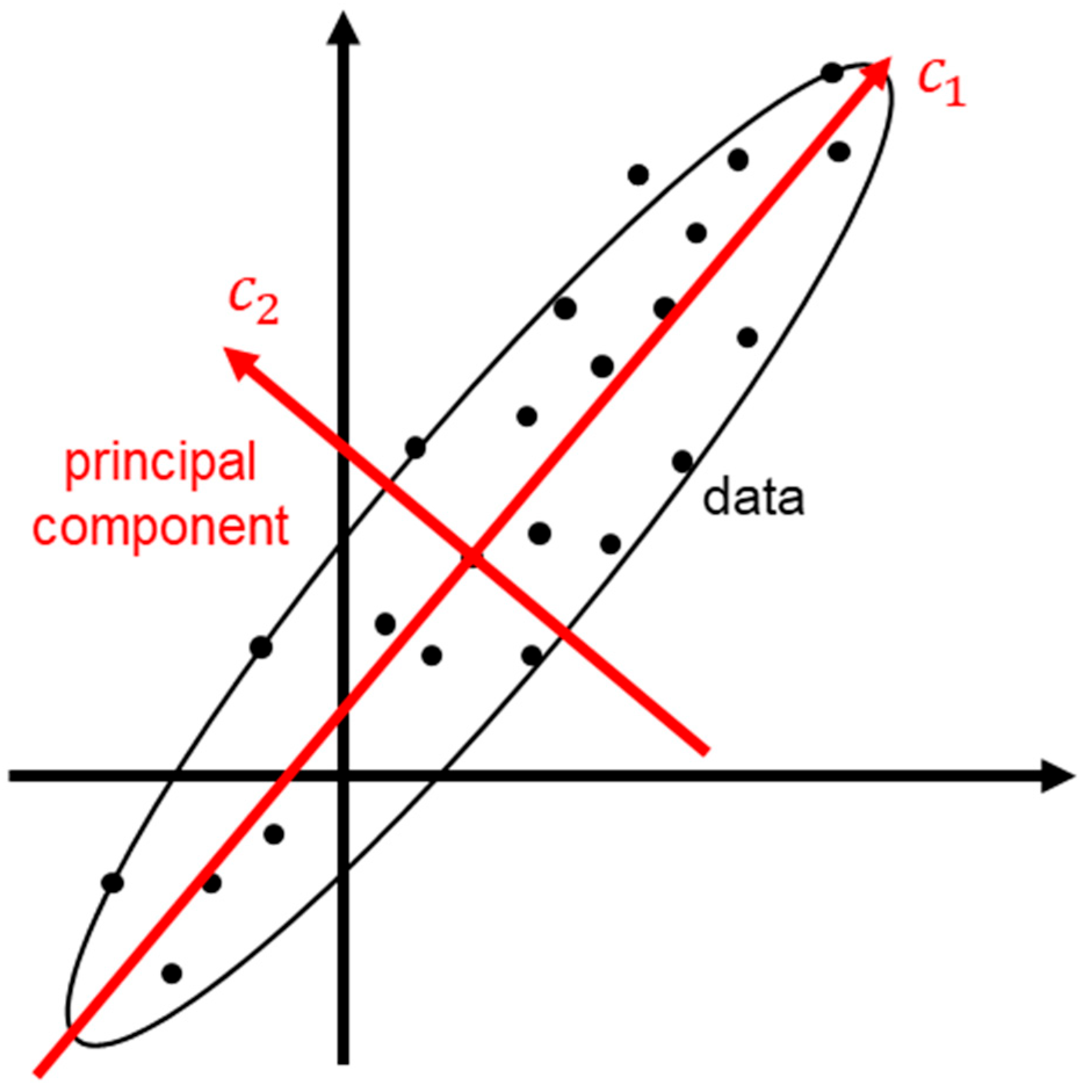
• Multipath Extraction: Apply PCA to the multi-day single-difference residuals to extract the multipath error signal (Section 2.2).
• Sky Grid Partitioning: Divide the station’s sky into grids based on specified intervals and assign the extracted multipath errors to their corresponding grid cells.
• Trend Surface Fitting: Within each grid cell, perform trend surface fitting on the multipath error values (as described in Section 2.3) to build the T-MHM model. Conduct statistical validation of the fitted model; if a fit is not statistically valid, use the mean error in that cell instead.
• Calculating Correction: Determine the satellite elevation and azimuth angles to locate the appropriate grid cell, then compute multipath corrections using either the stored polynomial coefficients or the mean error value.
• Final Positioning: Apply the computed multipath corrections to GNSS observations and perform least-squares estimation to obtain the final positioning results.

The specific GNSS data processing strategies used in this study are summarized in

Table 1. GNSS data processing strategies.

Parameters	Strategies
Observations	GPS L1/L2 BDS B1I/B2I
Ephemeris	GNSS broadcast ephemeris
Sampling interval	10 s
PCO/PCV	Model correction (igs14_2196.atx) [51]
Tropospheric delay	GPT2w+ Saastamoinen
Tropospheric delay projection function	GMF
Ionospheric delay	Double difference elimination
Ambiguity fixing	LAMBDA [52]

.

3. Results

3.1. Analysis of the Spatiotemporal Repeatability of Satellite Residuals

Before extracting multipath signals from the residuals, we first examine the spatiotemporal repeatability of the single-difference residuals for different satellites. This repeatability is a key assumption for our multi-day analysis. Figure 4 shows examples of single-difference residual time series for selected satellites on three different days (Day 001, 002, and 008 of year 2020). The first and second columns in the figure show the time series plots for GPS and BDS satellites, respectively, where “G” denotes GPS satellites and “C” represents BDS satellites. Three distinct colors correspond to the residual time series from the three different days. Since satellite orbital periods are not strictly aligned with a 24 h cycle, the time series have been temporally aligned to facilitate direct comparison across days.

For GPS satellites, which have a revisit period of approximately one sidereal day, the residual sequences show a clear cross-day correlation. As illustrated by the GPS example in Figure 4 (e.g., satellite G02 or G12), the single-difference residuals exhibit similar patterns on Days 001, 002, and 008, indicating significant repeatability. However, the residuals do not align perfectly across the three days. In addition to random noise, other non-multipath signals appear to be present, causing occasional deviations in the single-day residuals compared to the other two days (e.g., as highlighted by the gray-shaded region in the G02 plot).

For BDS satellites, the situation is more complex because the BDS constellation includes three types of orbits: Geostationary Earth Orbit (GEO), Inclined Geosynchronous Satellite Orbit (IGSO), and Medium Earth Orbit (MEO). Each type exhibits different repeat characteristics:

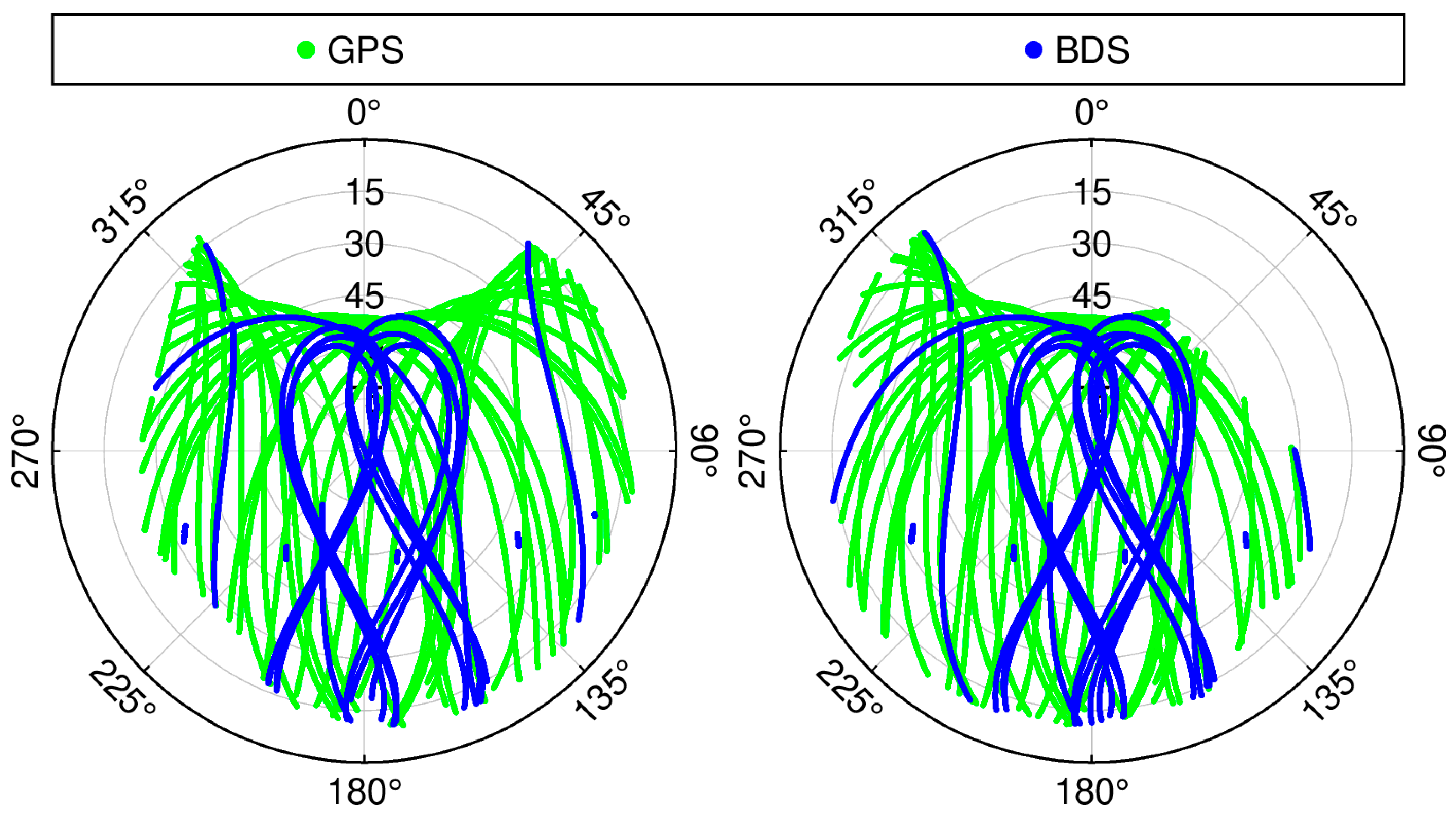
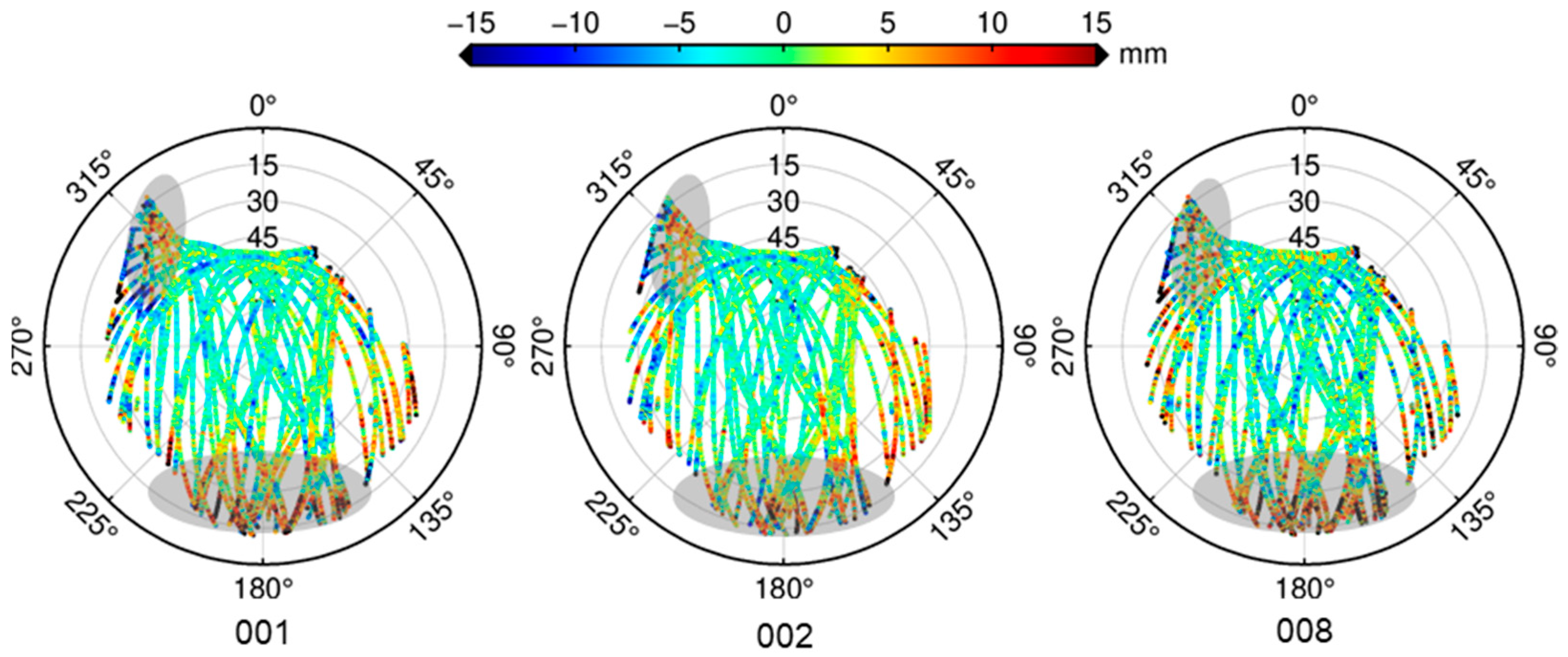
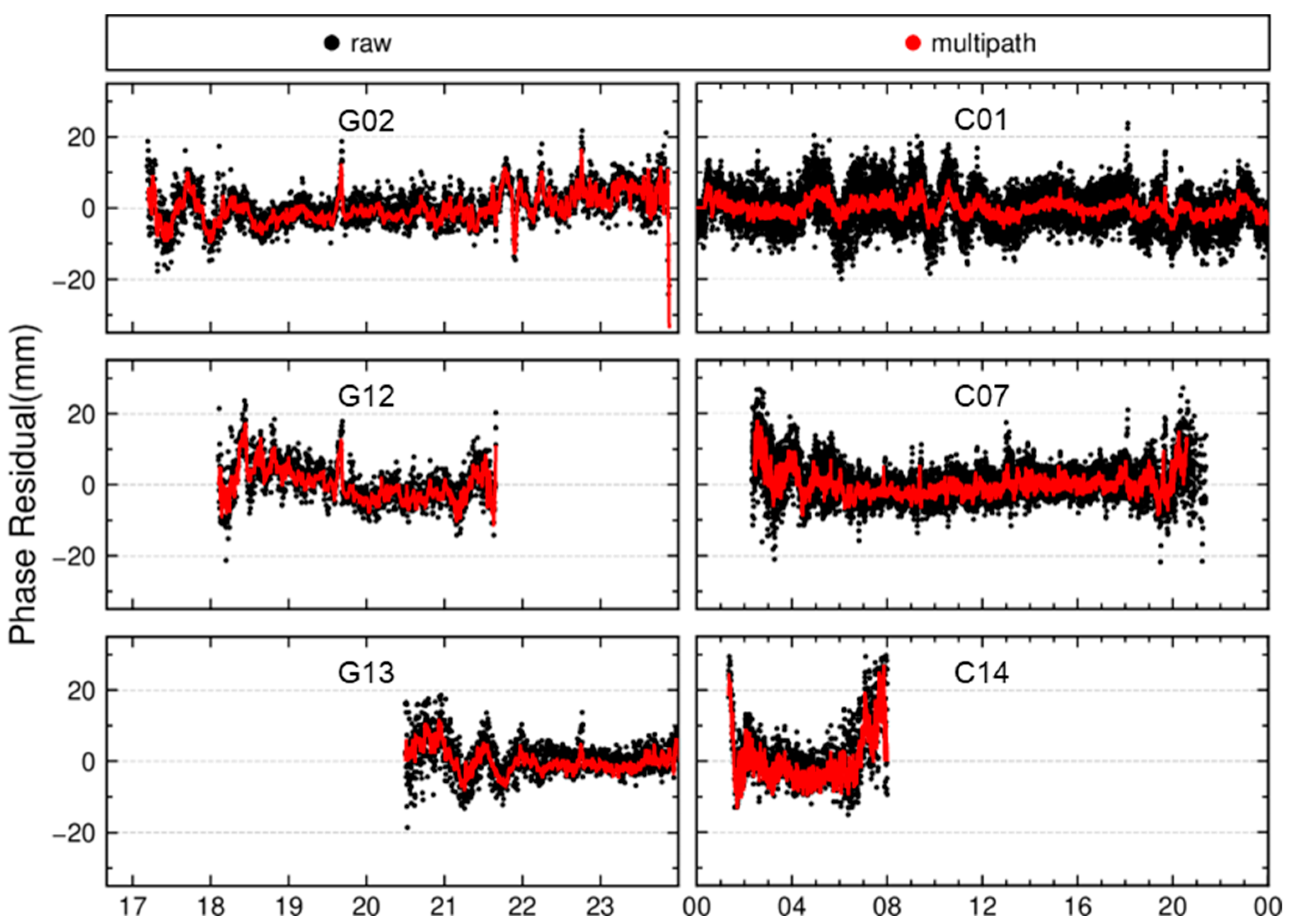
• GEO satellites (e.g., C01) orbit synchronously with Earth’s rotation, resulting in minimal positional variation over the station. As shown in the C01 time series (Figure 4), the GEO satellite is visible throughout the day from the station. One would expect its multipath errors to be relatively stable over time due to its static geometry. However, the residuals exhibit significant temporal trends and cross-day inconsistencies, suggesting the presence of additional unmodeled error sources.
• IGSO satellites (e.g., C07) follow a figure-eight ground track, covering a larger area than GEO satellites. For a station at mid-latitudes (such as in China), the IGSO satellites is visible during most of the day and repeats its ground track approximately every sidereal day. As expected, the C07 residuals exhibit strong repeatability on consecutive days (Figure 4), similarly to the GPS case.
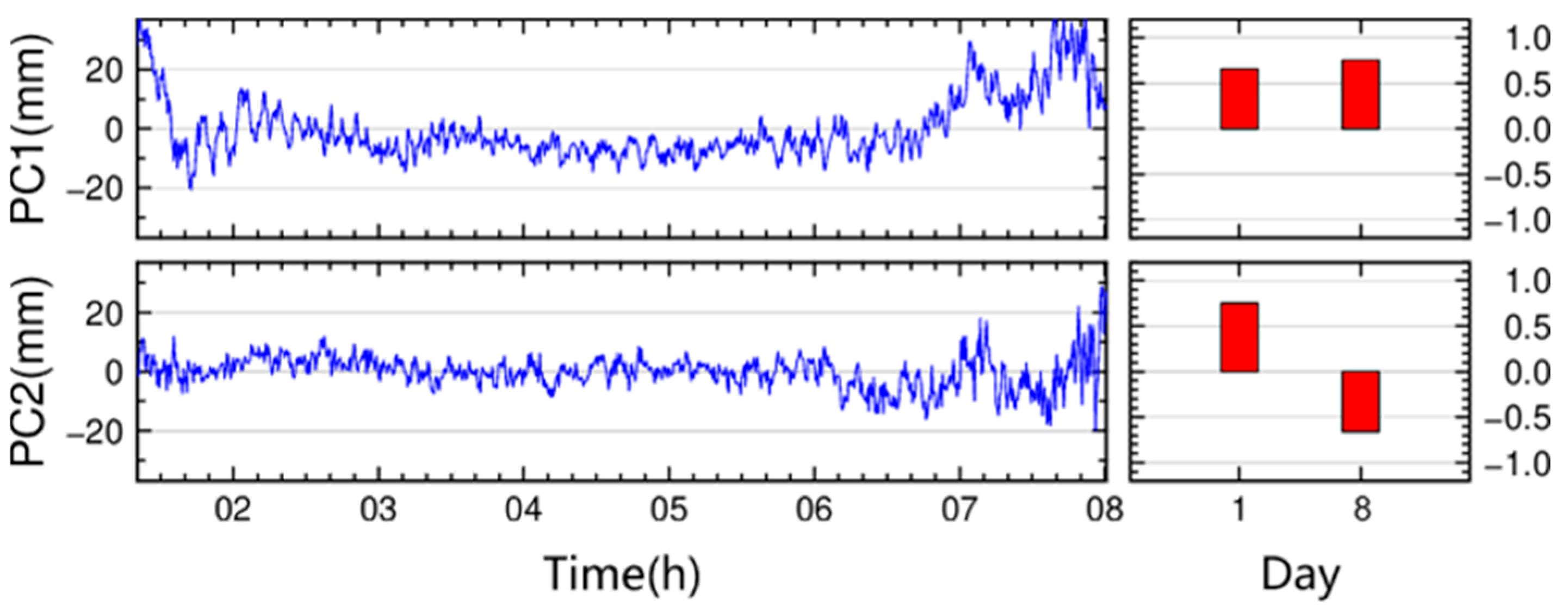
• MEO satellites (e.g., C14) have a longer revisit period of about seven sidereal days. The C14 residuals in Figure 4 illustrate that residual patterns on Day 001 vs. Day 002 (adjacent days) differ significantly in both shape and time coverage (because the satellite’s pass times differ), whereas Day 001 vs. Day 008 (seven days apart) show much higher correlation and more similar trends. This is consistent with the ~7-day repeat cycle for BDS MEO orbits.

To further investigate the spatial characteristics of the residuals, Figure 5 shows the single-difference residual sky plots from satellites on days 001, 002, and 008. The spatial distribution reveals that when the elevation angle is below approximately 45°, the absolute values of residuals mostly exceed 5 mm, indicating poor monitoring conditions at this station. Furthermore, compared to other regions above 30° elevation, residuals in the station’s northeastern obstructed zone (around 45° elevation and 30°–60° azimuth) show significantly higher magnitudes. This highlights that, in deformation monitoring environments, observation quality cannot be evaluated based solely on elevation angle. Additionally, as indicated by the shaded areas in the figure, the single-difference residuals display larger values in two distinct regions: the southern sky and northwestern sky of the station. The sky plots across the three days display consistent patterns, indicating a certain degree of spatial repeatability in the residual distribution.

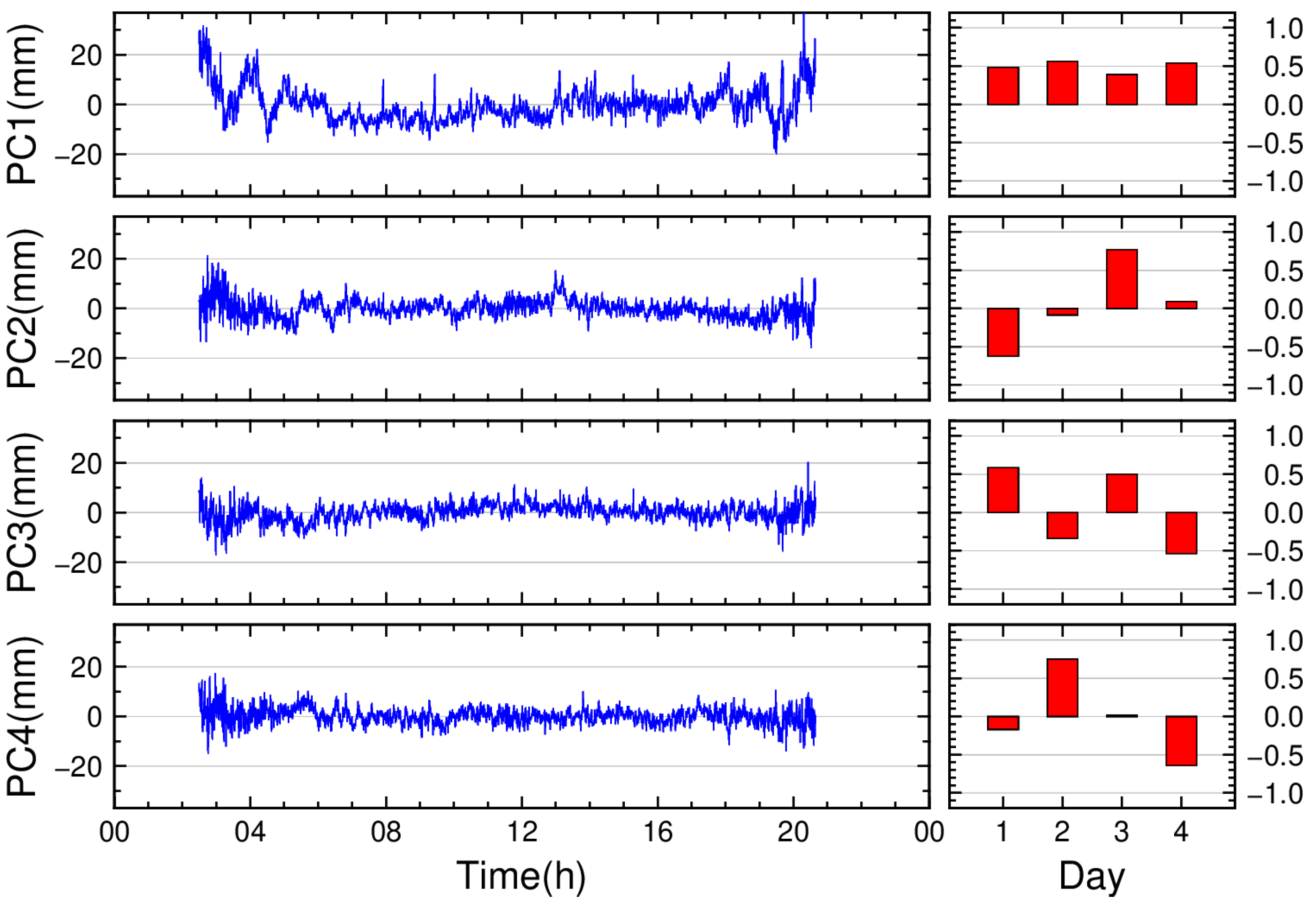
3.2. Identification of Multipath Errors in Residual Signals

With evidence of cross-day residual repeatability, we proceed to isolate the multipath error component using the PCA-based method. Except for BDS MEO satellites, we utilized four days of data for each satellite to perform PCA, decomposing the residuals into four PCs. Due to the unique characteristics of BDS MEO satellites, which require data separated by 7-day intervals for multipath error extraction, and the limited dataset spanning only 14 days in this study, only two days of data could be utilized for BDS MEO satellites, resulting in two decomposed PCs. Figure 6, Figure 7, Figure 8 and Figure 9 present the PCA results of single-difference residuals for selected satellites. In each figure, each row corresponds to a principal component: the left column shows the temporal patterns of the PCs, while the right column displays their corresponding daily coefficients.

Taking the GPS satellite G12 as an example, Figure 6 shows the PCA results of its single-difference residuals. The analysis reveals that the first PC (PC1) exhibits the largest amplitude and most distinct variations, while the subsequent components exhibit progressively smoother changes. This suggests that PC1 captures the dominant variation characteristics of the single-difference residuals. Furthermore, the daily coefficients of PC1 remain nearly constant across multiple days, stabilizing around 0.5 with a maximum variation of 0.04, while the coefficients of other PCs display significant day-to-day fluctuations. These properties confirm that PC1 aligns with the characteristics of multipath errors. During modeling, the multipath error values are derived by multiplying PC1 with the averaged multi-day coefficients of PC1.

For BDS satellites, Figure 7, Figure 8 and Figure 9 show the PCA results for the GEO (C01), IGSO (C07), and MEO (C14) satellites, respectively. Compared to GPS satellites:

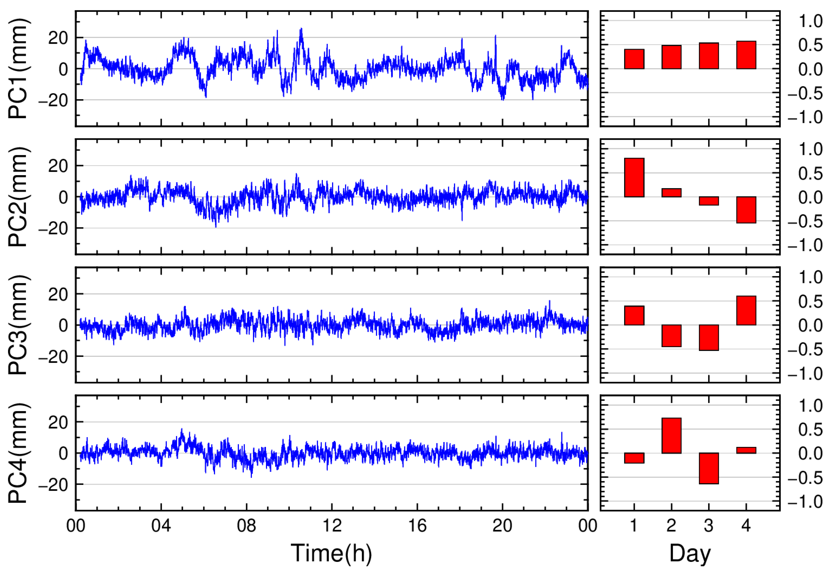
• BDS GEO satellites: The daily coefficients of PC1 exhibit minor variations across days (maximum difference: 0.16), with a multi-day average of 0.50.
• BDS IGSO satellites: The daily coefficients of PC1 show a maximum difference of 0.17 between days, averaging 0.50.
• BDS MEO satellites: The two-day coefficient difference for PC1 is 0.09, with an average of 0.7.

While BDS satellites demonstrate slightly larger day-to-day variations in PC1 coefficients compared to GPS satellites, these coefficients remain stable overall without significant deviations. Thus, for all these satellite types, PC1 can be reliably interpreted as the multipath error component. This consistency supports the validity of using PC1 to model multipath effects across all satellite types in the study.

To quantify the contribution of PC1 versus other components,

Table 2. Contribution of different PCs to the residual variance for representative satellites.

	G02	G12	G13	C01	C07	C14
PC1	71.0%	73.0%	57.2%	48.3%	53.5%	77.8%
PC2	13.6%	15.0%	18.5%	21.6%	18.1%	22.2%
PC3	9.3%	6.5%	15.2%	15.8%	14.7%	/
PC4	6.0%	5.4%	9.0%	14.3%	13.7%	/

lists the contribution ratios of different PCs to the residuals for each satellite type. The results indicate that PC1 accounts for the largest proportion of the residuals, confirming its role as the dominant component. Notably, the lower contribution of PC1 for BDS GEO satellites suggests that multipath effects are less significant in their residuals, with unmodeled errors (e.g., systematic biases or environmental interference) playing a larger role. In contrast, the high contribution rates of PC1 for GPS and BDS MEO satellites (75.0% and 77.4%, respectively) highlight that multipath errors dominate their residual patterns. This validates the feasibility of isolating and modeling multipath errors using PC1 and its corresponding eigenvectors. The stability and dominance of PC1 across all satellite types further reinforce its utility as a robust indicator for multipath characterization in deformation monitoring applications.

Figure 10 illustrates the comparison between the PCA-identified multipath errors and the original residuals. In the plot, black dots represent the raw residuals, while red dots denote the multipath errors identified via PCA. The results demonstrate that the separated multipath errors largely correspond to common variation trends observed in the multi-day residuals. Figure 11 displays the residual time series after removing the multipath errors. The plots reveal that significant variations in the residuals of all satellite types have been effectively eliminated post-correction, with the time series becoming notably smoother and fluctuating around zero. However, consistent with the findings in Table 2, the correction efficacy for BDS GEO satellites remains poor compared to other satellite types. Even after removing the multipath errors, the residual time series for GEO satellites retain higher volatility. This is attributed to the limited orbital motion of GEO satellites relative to the monitoring station, which confines multipath errors to minor fluctuations within a restricted spatial range. Consequently, multipath effects contribute less dominantly to GEO residuals compared to MEO and IGSO satellites. This inherent limitation reduces the effectiveness of multipath corrections for GEO satellites in deformation monitoring applications.

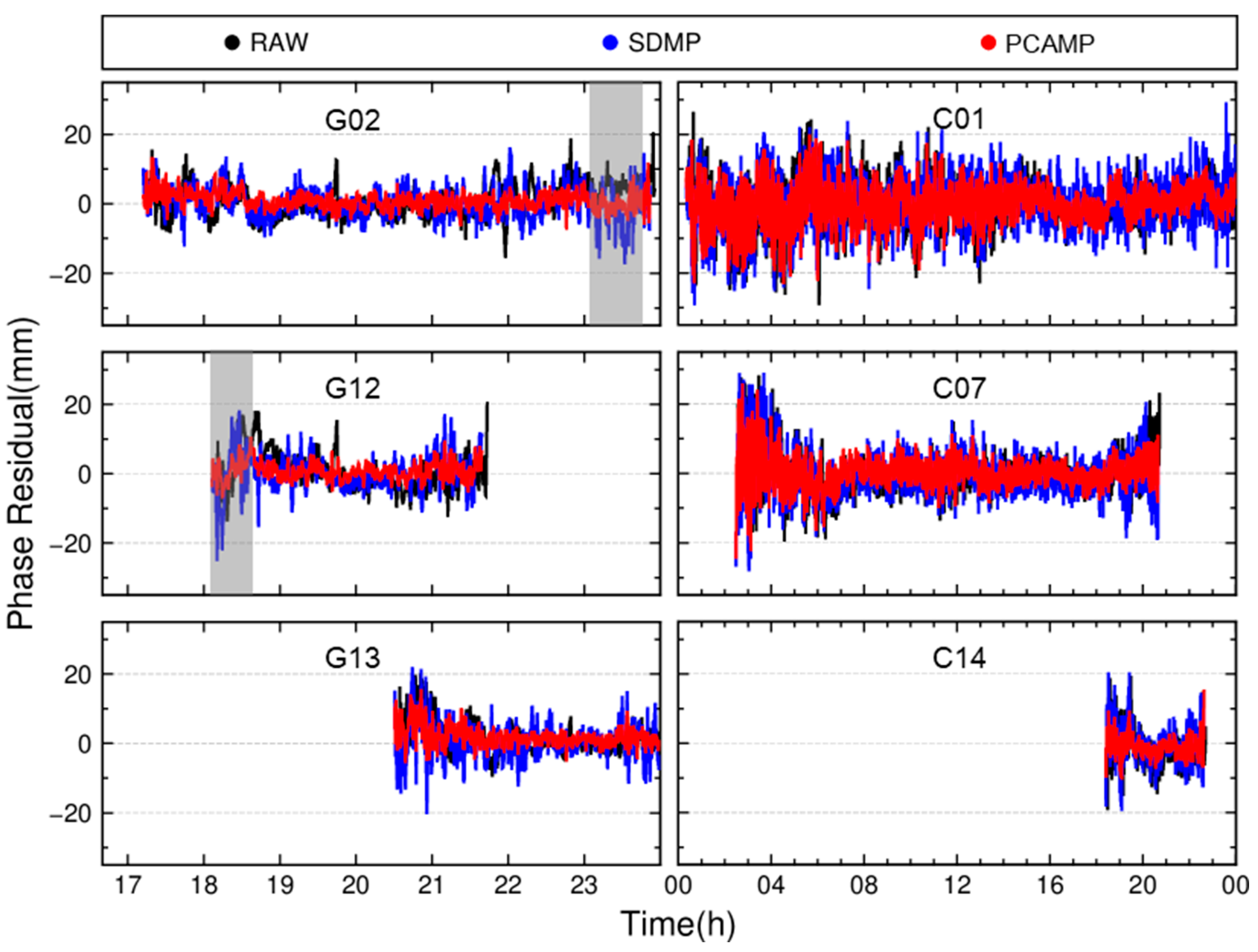
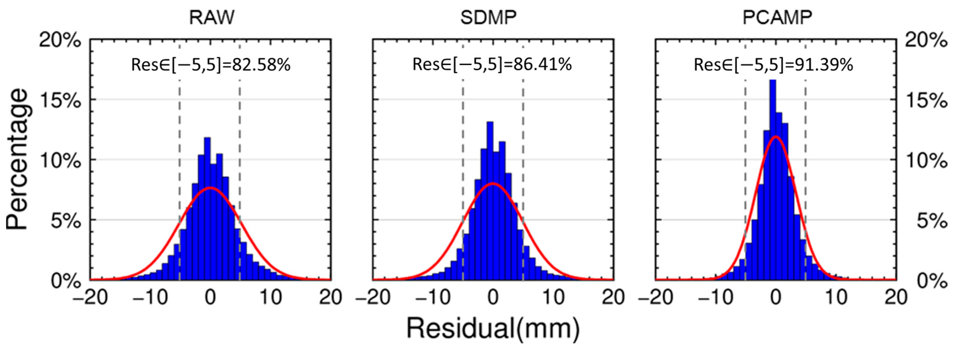
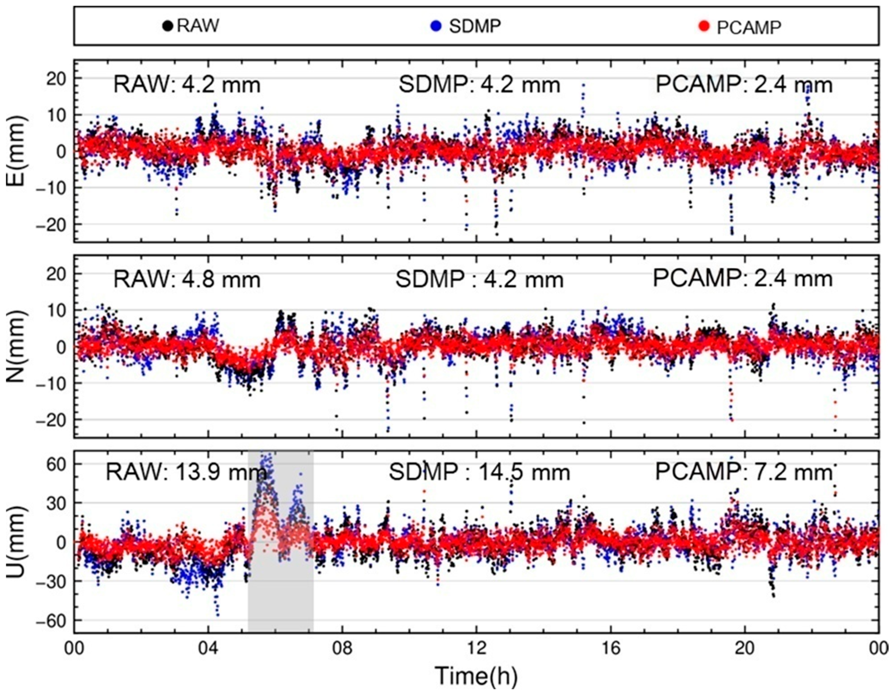
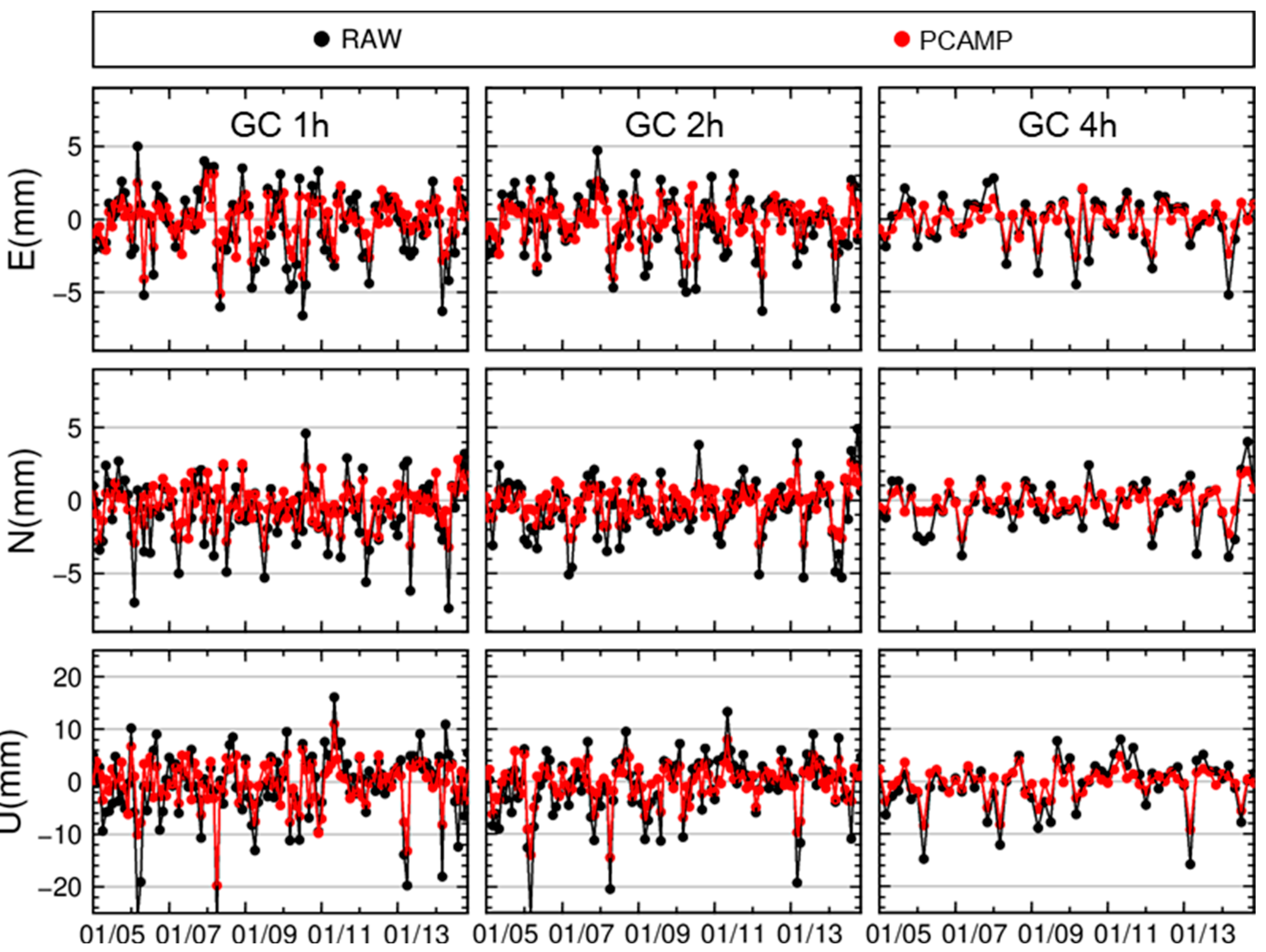
3.3. Model Correction and Positioning

To verify and analyze the correction effect of the model, this section adopts three different multipath error correction strategies to perform dynamic solution on the data of day 006. The specific solution strategies are shown in

Table 3. Strategies for multipath error correction.

Strategy	Content
RAW	No multipath correction
SDMP	Use Day 005 post-fit residuals as multipath errors estimates to correct Day 006 observations
PCAMP	Identify multipath errors via PCA from Days 001–004 residuals and correct Day 006 observations using the T-MHM model

. Among them, the RAW strategy does not correct the multipath error in the observations; the SDMP is the commonly used multipath error correction strategy at present, which assumes that the post-fit residuals only contain observation noise and multipath error; the PCAMP is the method introduced in the previous section, which performs PCA analysis on the post-fit residuals of multiple days to identify and correct the multipath error.

Figure 12 compares the residual time series of different satellite types after applying various correction strategies. In the figure, black, blue, and red represent the single difference residuals of satellites after RAW, SDMP, and PCAMP corrections and solutions, respectively. The residual time series of the same satellite across different days have been temporally aligned to facilitate comparison. The results show that the SDMP correction offers limited improvement—in some cases, particularly in the shaded areas of the figure, the SDMP-corrected residuals are even larger than those of the uncorrected (RAW) case, exhibiting more intense variations. This suggests that, in the deformation monitoring environment studied here, inter-day residuals are not solely composed of multipath effects and observation noise. When using residuals from the previous day for modeling and correction, unmodeled errors specific to that day can be introduced into the current day’s corrections. In contrast, the residuals after PCAMP correction are more stable, significantly eliminating the trend in the RAW residuals, and no significant correction errors have occurred. The results show that compared with SDMP, the PCA method can effectively extract multipath errors and correct them.

In addition, the correction effects of different types of satellites are inconsistent. After correction, the amplitude of the post-correction residuals of GPS satellites has decreased from 35 mm to about 20 mm. For BDS satellites, the amplitude of the post-correction residuals of GEO satellites has decreased from 57 mm to about 43 mm, that of IGSO satellites from 58 mm to about 49 mm, and that of MEO satellites from 38 mm to about 25 mm. The correction effects of the GPS and BDS MEO satellites are similar, and after correction, the amplitudes of the residuals have significantly decreased. After correction, although the amplitudes of the time series of the IGSO and GEO satellites have decreased, the post-correction time series still retain some trends and have relatively large amplitudes, indicating limited correction effects.

Table 4. Average RMS (mm) of single-difference residuals after applying different correction strategies.

	GPS	BDS
		GEO	IGSO	MEO
RAW	5.5	6.1	5.9	5.0
SDMP	4.8	6.0	5.8	4.3
PCAMP	2.8	5.5	4.3	2.9

shows the average RMS values of the post-fit residuals for different types of satellites after applying various correction strategies. Compared with the uncorrected (RAW) case, the SDMP correction offers only moderate improvement for GPS satellites, reducing RMS by approximately 13%, while having a little effect on BDS satellites, especially GEO and IGSO. In contrast, the PCAMP strategy significantly reduces RMS values across all satellite types. Specifically, PCAMP achieved reductions of 49%, 10%, 27%, and 42% for GPS, BDS GEO, BDS IGSO, and BDS MEO satellites, respectively, demonstrating its effectiveness in mitigating multipath effects. Among different satellite types, GPS and BDS MEO satellites exhibit the most significant PCAMP correction benefits. This is largely due to their wider orbital coverage, greater variation in satellite-station geometry, and generally higher signal quality, which makes multipath a dominant component of their residuals. In contrast, BDS GEO satellites, which remain nearly stationary relative to ground stations, contribute less multipath error, resulting in comparatively minimal correction effects.

Figure 13 illustrates the distribution of the single-difference residuals for all satellites after applying different correction strategies. It can be observed that the residual distributions under SDMP and PCAMP are more concentrated compared to RAW. The proportions of residuals with absolute values smaller than 5 mm for RAW, SDMP, and PCAMP are 82.58%, 86.41%, and 91.39%, respectively. Compared with RAW, SDMP only increases the proportion of residuals below 5 mm by 3.83%, indicating limited improvement. In contrast, residuals corrected by PCAMP are evidently closer to zero. PCAMP increases the proportion of residuals below 5 mm by 8.81% compared to RAW, demonstrating a far more substantial correction effect.

Figure 14 presents sky plots of single-difference residuals after applying different correction strategies. In the plots, residual points colored closer to green indicate smaller residual values, while those approaching red or blue represent larger residuals. The SDMP correction moderately improves the single-difference residuals, with some larger residuals in RAW being corrected. However, spatially correlated errors persist in the residual sky plot, particularly in low-elevation regions where red and blue points remain prominent. Notably, the residuals for some satellites at specific epochs even exceed those in RAW, suggesting the influence of day-to-day unmodeled errors on the results. In contrast, the PCAMP residual sky plot demonstrates significantly better performance, with most residuals colored green, indicating values close to zero. Except for residuals in the southern sky and plot edges, larger residuals in PCAMP show weak correlations with elevation or azimuth angles and lack distinct spatial patterns, being nearly uniformly distributed above 30° elevation. This implies that the remaining errors differ from multipath characteristics and likely represent other unmodeled errors specific to the observation day. Across all strategies, residuals in the southern sky consistently show relatively larger magnitudes and prove more difficult to mitigate, highlighting the complexity of error sources in that region.

Figure 15 shows the time series of dynamically fixed solutions coordinates for Day 006 under different correction strategies. The RMS values of the RAW coordinates in ENU directions are 4.2 mm, 4.8 mm, and 13.9 mm, respectively. After SDMP correction, the ENU RMS values become 4.2 mm, 4.2 mm, and 14.5 mm. In contrast, the PCAMP method achieves significantly better RMS values of 2.4 mm, 2.4 mm, and 7.2 mm. Compared with RAW, SDMP shows identical RMS in the E-direction, a 0.6 mm reduction in N-direction RMS, but a 0.6 mm increase in U-direction RMS. Notably, during specific epochs (e.g., gray-shaded regions in the figure), the SDMP coordinates exhibit larger deviations than RAW, particularly in the U-direction. These results suggest that under dam monitoring conditions, the day-to-day residual repeatability is insufficient. SDMP may introduce unmodeled errors beyond multipath effects, leading to incomplete or erroneous observation corrections that fail to improve positioning accuracy and even degrade performance at certain epochs.

In contrast, PCAMP reduces the RMS of coordinate time series by 1.8 mm (42.9%) in E-direction, 2.4 mm (50.0%) in N-direction, and 6.7 mm (48.2%) in U-direction compared to RAW. The PCAMP-corrected coordinate time series exhibit smoother variations compared to other methods, indicating effective mitigation of multipath effects. However, unlike ideal multipath modeling scenarios where residuals after correction typically manifest as white noise [53], the PCAMP-processed field data in this study retain residual variation trends resembling the original series. As discussed in the previous section, PCA-identified multipath errors account for 50–75% of total residuals, constituting the dominant component but leaving residual unmodeled errors. The remaining variations in the coordinate time series likely stem from day-specific unmodeled errors. This finding is consistent with the residual patterns observed in the sky plots, where persistent errors in the southern sky are linked to site-specific environmental factors.

In dam deformation monitoring, the static solutions are typically employed to achieve high positioning accuracy and reliability. This section evaluates positioning performance under static solutions with session lengths of 1 h, 2 h, and 4 h, comparing results before and after PCAMP corrections. As shown in Figure 16, positioning results across all session lengths demonstrate varying degrees of improvement after PCAMP corrections. The corrected time series exhibit reduced amplitude fluctuations and enhanced stability, with particularly notable enhancements in the U direction.

Table 5. RMS (mm) of coordinates before and after PCAMP correction for static positioning solutions of various session lengths, and the improvement (%).

	E			N			U
	RAW	PCAMP	Improvement	RAW	PCAMP	Improvement	RAW	PCAMP	Improvement
1 h	2.1	1.3	38.1	2.1	1.2	42.9	5.8	3.5	39.7
2 h	1.8	1.1	38.9	1.8	1.1	38.9	4.8	3	37.5
4 h	1.6	0.9	43.8	1.5	0.9	40	4.3	2.5	41.9

presents the RMS values of coordinates and their improvement before and after PCAMP multipath error correction. The results demonstrate significant mitigation effects, with average RMS reductions of 40.2%, 40.6%, and 39.7% in the East, North, and Up directions, respectively, showing comparable improvements across all components. Post-correction positioning accuracies reach 1.3 mm (horizontal) and 3.5 mm (vertical) for 1 h solutions, 1.1 mm (horizontal) and 3.0 mm (vertical) for 2 h solutions, and 0.9 mm (horizontal) and 2.5 mm (vertical) for 4 h sessions. Notably, the 2 h and 4 h sessions meet the submillimeter-level accuracy requirements for deformation monitoring applications. Similarly to the single-day kinematic solution results, PCAMP does not eliminate the variation trends in the time series, with some diurnal repeatability and systematic errors remaining—particularly evident in the U-direction. Based on the previous analysis, further investigation of the residuals from the perspective of other unmodeled errors may provide additional insights and improvements.

4. Conclusions

This study presented a refined GNSS multipath mitigation approach, termed PCA-based T-MHM, that incorporates the identification of multipath errors within GNSS residuals. The method addresses the limitations of traditional multipath mitigation methods in complex deformation monitoring environments by using a PCA framework to distinguish multipath signals from other residual errors and then modeling those signals with an enhanced T-MHM. We validated the approach using data from a dam deformation monitoring scenario, characterized by significant multipath due to reflective surroundings and obstructions.

Compared with conventional approaches, the PCA-based T-MHM method achieved significant reductions in residual error and corresponding improvements in positioning accuracy. In our experiments, the proposed model reduced the average post-fit residual RMS by approximately 49% for GPS, 10% for BDS GEO, 27% for BDS IGSO, and 42% for BDS MEO satellites, relative to no correction. The post-correction residuals displayed near-uniform spatial distributions on sky plots with reduced spatial correlations, confirming the method’s effectiveness in mitigating multipath errors. In terms of positioning performance, single-day kinematic solutions showed notable improvements: the RMS of the E, N, and U components decreased by 1.8 mm (42.9%), 2.4 mm (50.0%), and 6.7 mm (48.2%), respectively, enhancing dynamic positioning accuracy from the centimeter to the millimeter level. Static solutions (1 h, 2 h, and 4 h) demonstrated consistent RMS reductions across all E, N, and U components, averaging 40%, and achieved post-correction accuracies of 1.3 mm (horizontal) and 3.5 mm (vertical) for 1 h, 1.1 mm and 3.0 mm for 2 h, and 0.9 mm and 2.5 mm for 4 h sessions. These results meet or exceed the precision requirements for dam deformation monitoring and demonstrate the effectiveness of the method across both short and long observation spans.

While the PCAMP model significantly reduced multipath errors, minor systematic trends (e.g., residual daily signals and slight long-term drift, especially in the Up component) remained, suggesting contributions from other sources, such as residual atmospheric effects or site-specific biases [38]. Future work could explore advanced signal decomposition methods (e.g., wavelet transforms or Empirical Mode Decomposition) and refined atmospheric modeling to further enhance accuracy. Nevertheless, the proposed method represents a substantial advancement in multipath mitigation and can be readily integrated into high-precision GNSS deformation monitoring systems.

References

1. Groves, P.D.; Jiang, Z. Height Aiding, C/N-0 Weighting and Consistency Checking for GNSS NLOS and Multipath Mitigation in Urban Areas. J. Navig. 2013, 66, 653–669. [Google Scholar] [CrossRef]
2. Xue, Z.; Lu, Z.; Xiao, Z.; Song, J.; Ni, S. Overview of Multipath Mitigation Technology in Global Navigation Satellite System. Front. Phys. 2022, 10, 1071539. [Google Scholar] [CrossRef]
3. Brunner, F.K.; Hartinger, H.; Troyer, L. GPS Signal Diffraction Modelling: The Stochastic SIGMA-δ Model. J. Geod. 1999, 73, 259–267. [Google Scholar] [CrossRef]
4. Luo, X.; Mayer, M.; Heck, B. Improving the Stochastic Model of GNSS Observations by Means of SNR-Based Weighting. In Observing Our Changing Earth; Sideris, M.G., Ed.; Springer-Verlag Berlin: Berlin/Heidelberg, Germany, 2009; Volume 133, pp. 725–734. [Google Scholar]
5. Amiri-Simkooei, A.R.; Jazaeri, S.; Zangeneh-Nejad, F.; Asgari, J. Role of Stochastic Model on GPS Integer Ambiguity Resolution Success Rate. GPS Solut. 2016, 20, 51–61. [Google Scholar] [CrossRef]
6. Zhang, Q.; Zhang, L.; Sun, A.; Meng, X.; Zhao, D.; Hancock, C. GNSS Carrier-Phase Multipath Modeling and Correction: A Review and Prospect of Data Processing Methods. Remote Sens. 2024, 16, 189. [Google Scholar] [CrossRef]
7. Xi, R.; Meng, X.; Jiang, W.; An, X.; He, Q.; Chen, Q. A Refined SNR Based Stochastic Model to Reduce Site-Dependent Effects. Remote Sens. 2020, 12, 493. [Google Scholar] [CrossRef]
8. Bilich, A.; Larson, K.M.; Axelrad, P. Modeling GPS Phase Multipath with SNR: Case Study from the Salar de Uyuni, Boliva. J. Geophys. Res.-Solid. Earth 2008, 113, B04401. [Google Scholar] [CrossRef]
9. Benton, C.J.; Mitchell, C.N. Isolating the Multipath Component in GNSS Signal-to-Noise Data and Locating Reflecting Objects. Radio. Sci. 2011, 46, RS6002. [Google Scholar] [CrossRef]
10. Ge, L.; Han, S.; Rizos, C. Multipath Mitigation of Continuous GPS Measurements Using an Adaptive Filter. GPS Solut. 2000, 4, 19–30. [Google Scholar] [CrossRef]
11. Dai, W.; Ding, X.; Zhu, J.; Chen, Y.; Li, Z. EMD Filter Method and Its Application in GPS Multipath-All Databases. Acta Geod. Cartogr. Sin. 2006, 35, 321–327. [Google Scholar]
12. Tang, L.; Liang, S. Research on Multipath Correction of Observation Range Based on EEMD-MHM Model. Hydrogr. Surv. Charting 2022, 42, 54–58,64. [Google Scholar]
13. Yang, D.; Feng, W.; Huang, D.; Li, J. Improved Global Navigation Satellite System–Multipath Reflectometry (GNSS-MR) Tide Variation Monitoring Using Variational Mode Decomposition Enhancement. Remote Sens. 2023, 15, 4331. [Google Scholar] [CrossRef]
14. Zhong, P.; Ding, X.L.; Zheng, D.W.; Chen, W.; Huang, D.F. Adaptive Wavelet Transform Based on Cross-Validation Method and Its Application to GPS Multipath Mitigation. GPS Solut. 2008, 12, 109–117. [Google Scholar] [CrossRef]
15. Wang, Z. Research on GPS Multipath Effect Correction Technology in Urban Environment. Ph.D. Thesis, East China Normal University, Shanghai, China, 2020. [Google Scholar]
16. Genrich, J.; Bock, Y. Rapid Resolution of Crustal Motion at Short Ranges with the Global Positioning System. J. Geophys. Res.-Solid. Earth 1992, 97, 3261–3269. [Google Scholar] [CrossRef]
17. Zhong, P.; Ding, X.; Yuan, L.; Xu, Y.; Kwok, K.; Chen, Y. Sidereal Filtering Based on Single Differences for Mitigating GPS Multipath Effects on Short Baselines. J. Geod. 2010, 84, 145–158. [Google Scholar] [CrossRef]
18. Atkins, C.; Ziebart, M. Effectiveness of Observation-Domain Sidereal Filtering for GPS Precise Point Positioning. GPS Solut. 2016, 20, 123. [Google Scholar] [CrossRef]
19. Agnew, D.C.; Larson, K.M. Finding the Repeat Times of the GPS Constellation. GPS Solut. 2007, 11, 71–76. [Google Scholar] [CrossRef]
20. Choi, K.H.; Bilich, A.; Larson, K.M.; Axelrad, P. Modified Sidereal Filtering: Implications for High-Rate GPS Positioning. Geophys. Res. Lett. 2004, 31, L22608. [Google Scholar] [CrossRef]
21. Wang, M.; Wang, J.; Dong, D.; Li, H.; Han, L.; Chen, W. Comparison of Three Methods for Estimating GPS Multipath Repeat Time. Remote Sens. 2018, 10, 6. [Google Scholar] [CrossRef]
22. Lu, R.; Chen, W.; Zhang, C.; Li, L.; Peng, Y.; Zheng, Z. Characteristics of the BDS-3 Multipath Effect and Mitigation Methods Using Precise Point Positioning. GPS Solut. 2022, 26, 41. [Google Scholar] [CrossRef]
23. Lu, R.; Chen, W.; Li, Z.; Dong, D.; Jiang, W.; Wang, Z.; Huang, L.; Duan, X. An Improved Joint Modeling Method for Multipath Mitigation of GPS, BDS-3, and Galileo Overlapping Frequency Signals in Typical Environments. J. Geod. 2023, 97, 95. [Google Scholar] [CrossRef]
24. Cohen, C.E.; Parkinson, B.W. Mitigating Multipath Error in GPS Based Attitude Determination. In Proceedings of the Guidance and Control 1991; Proceedings of the Annual Rocky Mountain Guidance and Control Conference, Keystone, CO, USA, 2–6 February 1991; pp. 53–68. [Google Scholar]
25. Dong, D.; Wang, M.; Chen, W.; Zeng, Z.; Song, L.; Zhang, Q.; Cai, M.; Cheng, Y.; Lv, J. Mitigation of Multipath Effect in GNSS Short Baseline Positioning by the Multipath Hemispherical Map. J. Geod. 2016, 90, 255–262. [Google Scholar] [CrossRef]
26. Fuhrmann, T.; Luo, X.; Knoepfler, A.; Mayer, M. Generating Statistically Robust Multipath Stacking Maps Using Congruent Cells. GPS Solut. 2015, 19, 83–92. [Google Scholar] [CrossRef]
27. Cai, M.; Chen, W.; Dong, D.; Song, L.; Wang, M.; Wang, Z.; Zhou, F.; Zheng, Z.; Yu, C. Reduction of Kinematic Short Baseline Multipath Effects Based on Multipath Hemispherical Map. Sensors 2016, 16, 1677. [Google Scholar] [CrossRef]
28. Qu, L.; Jiang, W.; Li, J.; Du, Y.; Wang, H.; Wang, L.; Wang, J. Mitigation of Multipath Effects in Multi-GNSS and Multi-Frequency Precise Point Positioning with Multipath Hemispherical Maps. GPS Solut. 2024, 28, 1–13. [Google Scholar] [CrossRef]
29. Wang, Z.; Chen, W.; Dong, D.; Wang, M.; Cai, M.; Yu, C.; Zheng, Z.; Liu, M. Multipath Mitigation Based on Trend Surface Analysis Applied to Dual-Antenna Receiver with Common Clock. GPS Solut. 2019, 23, 104. [Google Scholar] [CrossRef]
30. Lu, R.; Chen, W.; Dong, D.; Wang, Z.; Zhang, C.; Peng, Y.; Yu, C. Multipath Mitigation in GNSS Precise Point Positioning Based on Trend-Surface Analysis and Multipath Hemispherical Map. GPS Solut. 2021, 25, 119. [Google Scholar] [CrossRef]
31. Zhan, W.; He, X.; Yuan, H.; Yang, H.; Zeng, J.; Jia, D. An Improved Multipath Mitigation Method Using Central Hemispherical Cell in Precise Point Positioning. Adv. Space Res. 2025, 75, 2721–2738. [Google Scholar] [CrossRef]
32. Zheng, K.; Tan, L.; Liu, K.; Chen, M.; Zeng, X. Assessing the Performance of Multipath Mitigation for Multi-GNSS Precise Point Positioning Ambiguity Resolution. Remote Sens. 2023, 15, 4137. [Google Scholar] [CrossRef]
33. Tao, Y.; Liu, C.; Tong, R.; Zhao, X.; Feng, Y.; Wang, J. Multipath Mitigation in Single-Frequency Multi-GNSS Tightly Combined Positioning via a Modified Multipath Hemispherical Map Method. Remote Sens. 2024, 16, 4679. [Google Scholar] [CrossRef]
34. Yuan, H.; Zhang, Z.; He, X.; Dong, Y.; Zeng, J.; Li, B. Multipath Mitigation in GNSS Precise Point Positioning Using Multipath Hierarchy for Changing Environments. GPS Solut. 2023, 27, 193. [Google Scholar] [CrossRef]
35. Zhang, R.; Gao, C.; Zhao, Q.; Peng, Z.; Shang, R. An Improved Multipath Mitigation Method and Its Application in Real-Time Bridge Deformation Monitoring. Remote Sens. 2021, 13, 2259. [Google Scholar] [CrossRef]
36. Chen, D.; Ye, S.; Xu, C.; Jiang, W.; Jiang, P.; Chen, H. Undifferenced Zenith Tropospheric Modeling and Its Application in Fast Ambiguity Recovery for Long-Range Network RTK Reference Stations. GPS Solut. 2019, 23, 26. [Google Scholar] [CrossRef]
37. Chen, D.; Ye, S.; Xia, F.; Cheng, X.; Zhang, H.; Jiang, W. A Multipath Mitigation Method in Long-Range RTK for Deformation Monitoring. GPS Solut. 2022, 26, 96. [Google Scholar] [CrossRef]
38. Lu, R.; Zhang, M.; Yuan, P.; Li, Z.; Chen, W.; Cai, M.; Chen, Y.; Dong, D.; Jiang, W. Enhancing Multi-GNSS Positioning Performances in Harsh Environments via a Refined Joint Troposphere-Multipath Hemispherical Map. GPS Solut. 2025, 29, 1. [Google Scholar] [CrossRef]
39. Liu, C.; Tong, R.; Tao, Y.; Chen, J.; Wang, J. A Deep Learning-Enhanced Observation-Domain Multipath Mitigation Study of BDS-3. Adv. Space Res. 2025, 75, 7049–7064. [Google Scholar] [CrossRef]
40. Tong, R.; Liu, C.; Tao, Y.; Wang, X.; Sun, J. ConvGRU-MHM: A CNN GRU-Enhanced MHM for Mitigating GNSS Multipath. Meas. Sci. Technol. 2024, 35, 045007. [Google Scholar] [CrossRef]
41. Guo, Z.; Yao, Y.; Xu, C.; Hu, M. Method for Establishing the Multipath Adaptive Mitigation Model Considering Deformation Displacement of Monitoring Stations. Geo-Spat. Inf. Sci. 2024, 1–16. [Google Scholar] [CrossRef]
42. Xu, C.; Guo, Z.; Yao, Y.; Hu, M.; Pan, P. A Multipath Mitigation Method for Significant Environmental Changes in Deformation Monitoring. Adv. Space Res. 2025, 75, 2753–2763. [Google Scholar] [CrossRef]
43. Pan, Y.; Möller, G.; Soja, B. Machine Learning-Based Multipath Modeling in Spatial Domain Applied to GNSS Short Baseline Processing. GPS Solut. 2024, 28, 1–13. [Google Scholar] [CrossRef]
44. Zhou, H.; Wang, X.; Zhong, S.; Xi, K.; Shen, H. A Multipath Hemispherical Map with Strict Quality Control for Multipath Mitigation. Remote Sens. 2025, 17, 767. [Google Scholar] [CrossRef]
45. Dong, D.; Fang, P.; Bock, Y.; Webb, F.; Prawirodirdjo, L.; Kedar, S.; Jamason, P. Spatiotemporal Filtering Using Principal Component Analysis and Karhunen-Loeve Expansion Approaches for Regional GPS Network Analysis. J. Geophys. Res.-Solid. Earth 2006, 111, B03405. [Google Scholar] [CrossRef]
46. He, X.; Hua, X.; Yu, K.; Xuan, W.; Lu, T.; Zhang, W.; Chen, X. Accuracy Enhancement of GPS Time Series Using Principal Component Analysis and Block Spatial Filtering. Adv. Space Res. 2015, 55, 1316–1327. [Google Scholar] [CrossRef]
47. Wdowinski, S.; Bock, Y.; Zhang, J.; Fang, P.; Genrich, J. Southern California Permanent GPS Geodetic Array: Spatial Filtering of Daily Positions for Estimating Coseismic and Postseismic Displacements Induced by the 1992 Landers Earthquake. J. Geophys. Res.-Solid. Earth 1997, 102, 18057–18070. [Google Scholar] [CrossRef]
48. Li, W.; Li, Z.; Jiang, W.; Chen, Q.; Zhu, G.; Wang, J. A New Spatial Filtering Algorithm for Noisy and Missing GNSS Position Time Series Using Weighted Expectation Maximization Principal Component Analysis: A Case Study for Regional GNSS Network in Xinjiang Province. Remote Sens. 2022, 14, 1295. [Google Scholar] [CrossRef]
49. Zheng, K.; Tan, L.; Liu, K.; Li, P.; Chen, M.; Zeng, X. Multipath Mitigation for Improving GPS Narrow-Lane Uncalibrated Phase Delay Estimation and Speeding up PPP Ambiguity Resolution. Measurement 2023, 206, 112243. [Google Scholar] [CrossRef]
50. Alber, C.; Ware, R.; Rocken, C.; Braun, J. Obtaining Single Path Phase Delays from GPS Double Differences. Geophys. Res. Lett. 2000, 27, 2661–2664. [Google Scholar] [CrossRef]
51. Schmid, R.; Steigenberger, P.; Gendt, G.; Ge, M.; Rothacher, M. Generation of a Consistent Absolute Phase-Center Correction Model for GPS Receiver and Satellite Antennas. J. Geod. 2007, 81, 781–798. [Google Scholar] [CrossRef]
52. Teunissen, P.J.G. The Least-Squares Ambiguity Decorrelation Adjustment: A Method for Fast GPS Integer Ambiguity Estimation. J. Geod. 1995, 70, 65–82. [Google Scholar] [CrossRef]
53. Chen, D. Research on BDS Medium/long-range Quickly Ambiguity Resolution and Regional Error Correction. Ph.D. Thesis, Wuhan University, Wuhan, China, 2016. [Google Scholar]
Figure 1. Schematic diagram of PCA.
Remotesensing 17 02694 g001
Figure 2. Sky plots of the stations (reference station on the left, monitoring station on the right).
Remotesensing 17 02694 g002
Figure 3. Data processing flowchart for multipath error modeling and correction.
Remotesensing 17 02694 g003
Figure 4. Single-difference residual time series for representative GPS and BDS satellites on Days 001, 002, and 008.
Remotesensing 17 02694 g004
Figure 5. Sky plots of satellite single-difference residuals for days 001, 002, and 008.
Remotesensing 17 02694 g005
Figure 6. PCA results of G12 single-difference residuals from days 001 to 004.
Remotesensing 17 02694 g006
Figure 7. PCA results of C01 single-difference residuals from days 001 to 004.
Remotesensing 17 02694 g007
Figure 8. PCA results of C07 single-difference residuals from days 001 to 004.
Remotesensing 17 02694 g008
Figure 9. PCA results of C14 single-difference residuals on days 001 and 008.
Remotesensing 17 02694 g009
Figure 10. Comparison of PCA-identified multipath error signal (red) with raw residuals (black) for a representative satellite.
Remotesensing 17 02694 g010
Figure 11. Single-difference residual time series after removing the identified multipath errors.
Remotesensing 17 02694 g011
Figure 12. Single-difference residual time series for various satellites after applying different correction strategies on day 006.
Remotesensing 17 02694 g012
Figure 13. Histogram of satellite single-difference residuals for all satellites under different correction strategies.
Remotesensing 17 02694 g013
Figure 14. Sky plot of satellite single-difference residuals.
Remotesensing 17 02694 g014
Figure 15. Coordinate time series from kinematic fixed solutions on day 006 under different multipath correction strategies.
Remotesensing 17 02694 g015
Figure 16. Coordinate time series of combined GPS+BDS static solutions for 1 h, 2 h, and 4 h sessions.
Remotesensing 17 02694 g016