Article

The First Step of AI in LEO SOPs: DRL-Driven Epoch Credibility Evaluation to Enhance Opportunistic Positioning Accuracy

1
Aerospace Information Research Institute, Chinese Academy of Sciences, Beijing 100080, China
2
School of Electronic, Electrical and Communication Engineering, University of Chinese Academy of Sciences, Beijing 101400, China
3
School of Information Science and Technology, Beijing University of Technology, Beijing 100124, China
*
Author to whom correspondence should be addressed.
These authors contributed equally to this work.
Remote Sens. 2025, 17(15), 2692; https://doi.org/10.3390/rs17152692
Submission received: 25 June 2025 / Revised: 26 July 2025 / Accepted: 28 July 2025 / Published: 3 August 2025
(This article belongs to the Special Issue LEO-Augmented PNT Service)

Abstract

Low Earth orbit (LEO) signal of opportunity (SOP) positioning relies on the accumulation of epochs obtained through prolonged observation periods. The contribution of an LEO satellite single epoch to positioning accuracy is influenced by multi-level characteristics that are challenging for traditional models. To address this limitation, we propose an Agent-Weighted Recursive Least Squares (RLS) Positioning Framework (AWR-PF). This framework employs an agent to comprehensively analyze individual epoch characteristics, assess their credibility, and convert them into adaptive weights for RLS iterations. We developed a novel Markov Decision Process (MDP) model to assist the agent in addressing the epoch weighting problem and trained the agent utilizing the Double Deep Q-Network (DDQN) algorithm on 107 h of Iridium signal data. Experimental validation on a separate 28 h Iridium signal test set through 97 positioning trials demonstrated that AWR-PF achieves superior average positioning accuracy compared to both standard RLS and randomly weighted RLS throughout nearly the entire iterative process. In a single positioning trial, AWR-PF improves positioning accuracy by up to 45.15% over standard RLS. To the best of our knowledge, this work represents the first instance where an AI algorithm is used as the core decision-maker in LEO SOP positioning, establishing a groundbreaking paradigm for future research.

Graphical Abstract

1. Introduction

Global Navigation Satellite Systems (GNSSs), as the most widely used positioning, navigation, and timing (PNT) solution [1], exhibit some inherent limitations [2]. The most critical limitation of GNSS signals is the relatively high orbital altitude (greater than 19,000 km) [3], which induces substantial signal path loss, resulting in low minimal received power (−155dBW–−163dBW) [4]. This inherent limitation leads to significantly degraded positioning performance or complete service outages in blocked environments such as urban canyons, dense foliage, tunnels, and indoor spaces [5]. Signal of opportunity-based (SOP-based) positioning has emerged as a promising alternative due to its non-cooperative texture, flexibility, and ubiquitous coverage. Recent studies have explored diverse signal sources, including amplitude modulation/frequency modulation radio broadcasts [6], Wi-Fi [7], fifth-generation cellular networks for mobile phones [8], digital television transmissions [9], and low Earth orbit (LEO) satellite signals [10]. Notably, LEO satellite signals have garnered extensive research attention due to their unique advantages: the presence of large constellations offering global coverage [11], rapidly evolving geometry [12], enhanced ground-received power [13], and pronounced Doppler frequency shifts [14]. Previous studies have achieved positioning accuracy ranging from meters to hundreds of meters by leveraging SOPs from single or multiple LEO satellite constellations [15,16,17,18].
LEO SOP positioning utilizes satellite position and velocity information derived from ephemeris extrapolation as spatiotemporal references, combined with Doppler frequency and timestamp measurements extracted from LEO signals to achieve positioning. However, LEO-SOP-based positioning also suffers from inherent limitations. At the satellite level, the error of Two-Line Element (TLE)-based orbit extrapolation models grows over time [19]. The geometric configuration of satellites, characterized by their elevation and azimuth angles, directly influences the Geometric Dilution of Precision (GDOP). A lower GDOP value, resulting from favorable satellite distributions, enhances positioning accuracy by reducing the sensitivity of results to observational errors. Conversely, an unfavorable configuration (e.g., satellites clustered in a narrow angular range) elevates GDOP, amplifying error propagation. At the epoch level, the LEO SOP positioning depends on capturing numerous epochs. The introduction of numerous similar epochs from the same satellite may lead to a near-singular observation matrix, resulting in severe degradation of positioning accuracy. At the signal level, the signal-to-noise ratio (SNR) and Doppler frequency exhibit severe fluctuations [20]. These inherent drawbacks in multiple levels of LEO SOPs limit positioning accuracy.
To mitigate the aforementioned inherent limitations of LEO opportunistic signals, significant research efforts have been made. In 2023, an Orbit Error Compensation and Weighting (OECW) method was proposed to compensate for Doppler frequency errors caused by orbital inaccuracies at each epoch, achieving a 70% improvement in horizontal positioning accuracy [21]. In 2024, a closed-loop machine learning model for LEO satellite orbit prediction was proposed, effectively reducing predicted orbital errors [22]. Compared to orbits predicted using the Simplified General Perturbations Version 4 (SGP4) model, the proposed model-based prediction improved LEO SOP positioning accuracy by 84.6%. In 2023, a comprehensive analysis was conducted on the influence of baseline in LEO SOP differential Doppler positioning [23]. The study achieved a 3D positioning accuracy of 122.1 m for long-baseline scenarios and 1.9 m for zero-baseline cases. At the satellite level, extensive research has been conducted on multi-constellation fusion to optimize the limited geometric configurations inherent in single-constellation systems. In 2024, a research team from Curtin University achieved positioning accuracy of approximately 10 m by performing Doppler-based joint positioning using SOPs from the Starlink, OneWeb, and Iridium constellations [24]. In 2024, a study employing a differential architecture analyzed and compensated for LEO satellite ephemeris errors [25]. In the integrated positioning experiment combining LEO opportunistic signals with an Inertial Navigation System (INS), the system achieved an average Root Mean Square Error (RMSE) of 11.74 m and a final positioning error of 12.01 m. At the signal level, some research achievements have been made to address the limitations of LEO SOPs, including the short availability of signal duration, irregular acquisition times, and large SNR fluctuations. In 2020, a research team from Tsinghua University developed an algorithm utilizing implicit pilot signals in Iridium SOP to enhance Doppler frequency estimation accuracy, achieving a 70% improvement in Doppler estimation accuracy [26]. That same year, a novel Quadratic Square Accumulating Instantaneous Doppler Estimation (QSA-IDE) algorithm was proposed to improve Doppler estimation accuracy under weak signal conditions [27]. Experimental results demonstrated that this algorithm achieved a 2D average positioning error of 163 m, representing a 17 m improvement over conventional methods. In 2022, the same research team further refined their approach by proposing a “phase-time” algorithm that leveraged entire Iridium signal frames rather than just pilot segments for Doppler estimation [28]. Through 800 positioning experiments, this enhanced algorithm was shown to improve positioning accuracy by 31.57–42.81% compared to traditional methods. However, existing studies remain confined to single-factor optimization (satellite/epoch/signal level) and lack joint modeling capability for fusing-level error coupling mechanisms. More fundamentally, conventional methods cannot perceive single-epoch-level signal degradation in real time, leading to severely compromised positioning robustness in complex dynamic scenarios. This paper aims to resolve this core challenge.
This study systematically analyzes multi-level factors affecting LEO SOP positioning accuracy and proposes an innovative Agent-Weighted Recursive Least Squares (RLS) Positioning Framework (AWR-PF). The proposed framework employs an agent to evaluate the credibility of multi-level characteristics and decides epoch weights for real-time RLS iteration. Leveraging the inherent temporal dependency of RLS algorithms, our approach incorporates previously overlooked critical dimensions—epoch arrival sequence and inter-epoch dependencies. Unlike conventional “snapshot” processing, our framework treats positioning as a continuous decision-making process where each epoch generates a positioning state and the agent’s weighting actions directly influence future positioning states.
Our agent learns to predict how current epoch weighting affects future positioning accuracy based on historical epochs. This epoch weighting problem involves complex environmental conditions and strong inter-epoch decision dependencies. Since Deep Reinforcement Learning (DRL) excels at handling sequential decision-making under uncertainty [29], we adopt DRL to address this challenge. To enable DRL-based training, we formulate the positioning problem as a Markov Decision Process (MDP) with multi-dimensional states and discrete actions, effectively transforming it into a model suitable for deep reinforcement learning. As illustrated in Table 1, this MDP model trains an agent to optimize LEO SOP positioning performance through sequential decision-making.
As an advanced DRL method, Double Deep Q-Network (DDQN) effectively mitigates overestimation bias by decoupling action selection from value estimation [30]. This method enables dynamic and precise epoch weight allocation, making it particularly suitable for multi-factor, noise-corrupted weighting scenarios in LEO SOP positioning.
Building upon the DDQN, we developed the DDQN-based Epoch Weighting (DDQN-EW) algorithm by (1) employing a lightweight neural network to extract positioning-relevant features across satellite, epoch, signal, and positioning layers; (2) designing collaborative interaction between the agent and RLS for weight-based decision-making; and (3) formulating a reward mechanism sensitive to positioning error convergence dynamics. This specialized architecture enables intelligent epoch-wise weighting while maintaining computational efficiency for real-time navigation applications.
We trained the agent using the DDQN-EW algorithm on a training set comprising 393,933 real Iridium epochs extracted from 107 h of continuous observation. The agent learns to perform real-time epoch weighting by integrating multiple epoch characteristics. Unlike traditional static epoch weighting and screening algorithms, the proposed approach learns policy directly from extensive empirical data to autonomously generate optimal weighting policy through DRL. During evaluation, the agent generates dynamic weights through real-time analysis of epoch characteristics (SNR/Doppler/elevation angle, etc.), which serve as adaptive factors in RLS positioning, thereby establishing a closed-loop optimization framework. Due to the agent’s comprehensive consideration of multi-level characteristics and temporal dependency-aware decision-making, the proposed AWR-PF demonstrates superior positioning accuracy throughout the entire recursive process compared to both standard RLS and randomly weighted RLS in experimental trials. The main contributions of this study are threefold:
  • Systematic analysis of multi-level characteristics affecting LEO SOP positioning accuracy based on numerous independent trials.
  • Proposal of a novel Agent-Weighted RLS Positioning Framework (AWR-PF), a pioneering application of artificial intelligence (AI) algorithms in LEO SOP positioning. By employing an agent trained on extensive real-world Iridium signal and comprehensively incorporating multiple positioning accuracy-influencing factors, our framework achieves superior positioning performance.
  • Definition of an innovative MDP model with precisely formulated states, actions, and rewards, effectively transforming practical opportunistic signal positioning problems into a model suitable for DRL algorithm training, thereby establishing a paradigm for intelligent algorithm applications in future LEO opportunistic signal positioning systems.
The remainder of this paper is organized as follows: Section 2 characterizes the Iridium signal epoch features that influence positioning accuracy. Section 3 presents the proposed Agent-Weighted RLS Positioning Framework. Section 4 presents the proposed MDP model and details the agent training process using the DDQN-EW algorithm. Section 5 analyzes the training and evaluation results. Section 6 presents some valuable discussions. Finally, Section 7 concludes the paper.

2. Characteristic Analysis of the Iridium System

This section comprehensively analyzes epoch characteristics in LEO SOP positioning from three perspectives: satellite, epoch, and signal levels. These characteristics collectively impact positioning accuracy and must be considered in the following algorithm design.

2.1. The Satellite Level

2.1.1. Error of Predicted Orbit

In LEO SOP scenarios, LEO satellite positions are typically obtained using TLE combined with orbit prediction models. However, existing orbit prediction models exhibit time-growing errors that degrade positioning performance. Doppler frequency serves as the fundamental observable element in LEO SOP positioning, which can be expressed as:
f d = f c c v r r
where f c denotes the carrier frequency, c denotes the speed of light, v denotes the velocity of satellite, and r denotes the distance vector from the satellite to the receiver. The huge orbital position and velocity prediction errors will result in Doppler frequency prediction errors of up to 15 Hz [31]—far exceeding the RMSE of refined Iridium Doppler estimation algorithms [32].
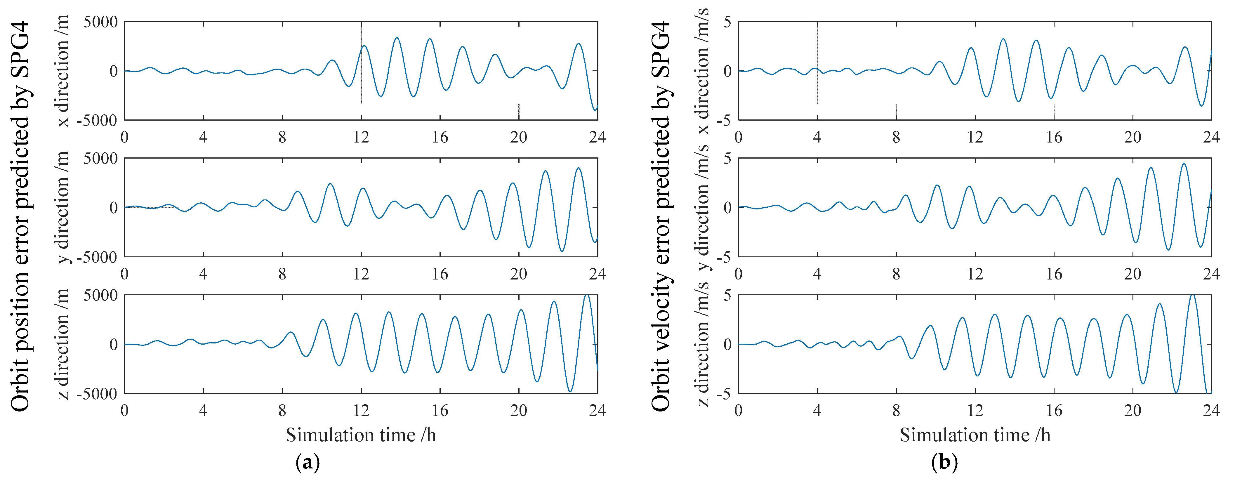
Figure 1 illustrates the simulation result of the 3D position and velocity errors of Iridium satellites predicted via the SGP4 over time. Within the first 8 h, the orbital errors remain relatively stable; beyond this period, errors increase dramatically. Therefore, the ephemeris age—defined as the time interval from the last ephemeris update to the epoch reception moment—quantifies the orbital prediction error for that specific epoch. As orbital errors constitute a significant error source in LEO SOP positioning, ephemeris age must be considered as a critical epoch characteristic.

2.1.2. The Orbital Configuration

The orbital configuration of satellites directly influences the linearity of the observation matrix in positioning solutions. Assume that in a LEO SOP Doppler positioning, a total of N e epochs are received; then the observation matrix G d o p p l e r can be defined as:
G D o p p l e r = ρ ^ ˙ x 1 / γ ρ ^ ˙ y 1 / γ ρ ^ ˙ z 1 / γ 1 ρ ^ ˙ x 2 / γ ρ ^ ˙ y 2 / γ ρ ^ ˙ z 2 / γ 1 ρ ^ ˙ x 3 / γ ρ ^ ˙ y 3 / γ ρ ^ ˙ z 3 / γ 1 ρ ^ ˙ x N e / γ ρ ^ ˙ y N e / γ ρ ^ ˙ z N e / γ 1
where ρ ^ ˙ x i , ρ ^ ˙ y i , and ρ ^ ˙ z i denote the rates of change of the pseudo-range direction vector of the i-th epoch in the x, y, and z directions, respectively (which can be derived using the SPG4 model). γ denotes the maximum rate of change of the pseudo-range direction vector, which is defined as:
γ = ρ ^ ˙ m a x = 1 1 ( Re / a o r b ) μ a o r b 3
where a o r b denotes the semi-major axis of the satellite orbit, Re donates the radius of the Earth, and μ denotes the gravitational constant, with a value of 398,600 × 109 m3/s2.
The dimensionless Doppler positioning cofactor array Q D o p p l e r from γ can be defined as:
Q D o p p l e r = G d o p p l e r T G d o p p l e r 1 = g 11 g 12 g 13 g 14 g 21 g 22 g 23 g 24 g 31 g 32 g 33 g 34 g 41 g 42 g 43 g 44
where the subscripts 1, 2, and 3 of g respectively represent the position estimates in the x, y, and z directions, and 4 represents the clock bias estimation. g 11 denotes the cofactor of the position estimation in the x direction, g 12 denotes the cofactor between the position estimation in the x direction and y direction, and so forth. The dimensionless analysis described above is termed generalized Doppler analysis, where the generalized Doppler geometry dilution of precision (GDOP) and its position dilution of precision (PDOP) can be expressed as [33]:
G D O P = g 11 + g 22 + g 33 + g 44
P D O P = g 11 + g 22 + g 33
The corresponding positioning accuracy can be expressed in terms of the PDOP as [34]:
σ r = P D O P λ σ D / γ
where σ r denotes the positioning error, σ D denotes the observable error of Doppler frequency, and λ denotes the wavelength of the carrier.
Therefore, unlike pseudo-range positioning, generalized Doppler GDOP requires not only diverse geometric distributions of satellites but also diverse velocity directions of satellites; that is, it has higher requirements for the diversity of orbits. More diverse Doppler projection directions can reduce the generalized Doppler GDOP and improve the Doppler positioning accuracy.

2.1.3. Elevation Angle/Azimuth Angle/Satellite-to-Receiver Distance

In LEO SOP positioning, epochs with distinct azimuth and elevation angles correspond to different velocity vectors. As discussed in Section 2.1.2, incorporating epochs with more diverse velocity vectors can improve PDOP and consequently enhances positioning accuracy. Therefore, both azimuth and elevation angles should be treated as critical epoch features for screening purposes.
Furthermore, variations in satellite-to-receiver distances lead to differing signal free-space path loss (FSPL), which can be expressed as:
L f s = 4 π d f c c 2
L f s dB = 20 log 10 d + 20 log 10 f c + 92.45
where d denotes the satellite-to-receiver distance and f c denotes the carrier frequency. A longer satellite-to-receiver distance results in greater FSPL, leading to degraded received signal quality. Therefore, it is essential to incorporate the satellite-to-receiver distance at the epoch reception time as a critical epoch characteristic.

2.2. The Epoch Level

The Phenomenon of Epoch Redundancy

In LEO SOP positioning, a large number of epochs are captured within each observation window. However, the limited number of orbital planes in LEO constellations results in many epochs originating from the same orbital plane or even the same satellite. This study makes a novel observation that introducing these similar epochs leads to a near-rank-deficient condition in the observation matrix, significantly degrading the noise resistance of positioning solutions. This phenomenon becomes particularly pronounced during short observation periods.
Here, we formally define epoch redundancy for LEO SOP positioning for the first time. Consider a positioning scenario where the total number of received epochs is N t o t a l , with N 1 , N 2 , …, N k representing the epoch counts from k individual satellites. Then the epoch redundancy for LEO SOP positioning can be defined as:
R e = max N 1 , N 2 , , N k i = 1 k N i = max N 1 , N 2 , , N k N t o t a l
Figure 2 presents the result from 500 real-world Iridium signal positioning trials. As the epoch redundancy increases, both GDOP and positioning errors exhibit more severe fluctuations. This confirms that the observation matrix has become ill-conditioned, rendering the position solutions highly sensitive to noise.
Therefore, in a positioning trial, the rank of an epoch within its parent satellite’s observation sequence becomes a significant feature worthy of consideration. A higher rank value indicates that more similar epochs from the same satellite have been received prior to this epoch, consequently reducing its utility value for positioning.

2.3. The Signal Level

2.3.1. The Fluctuation of SNR

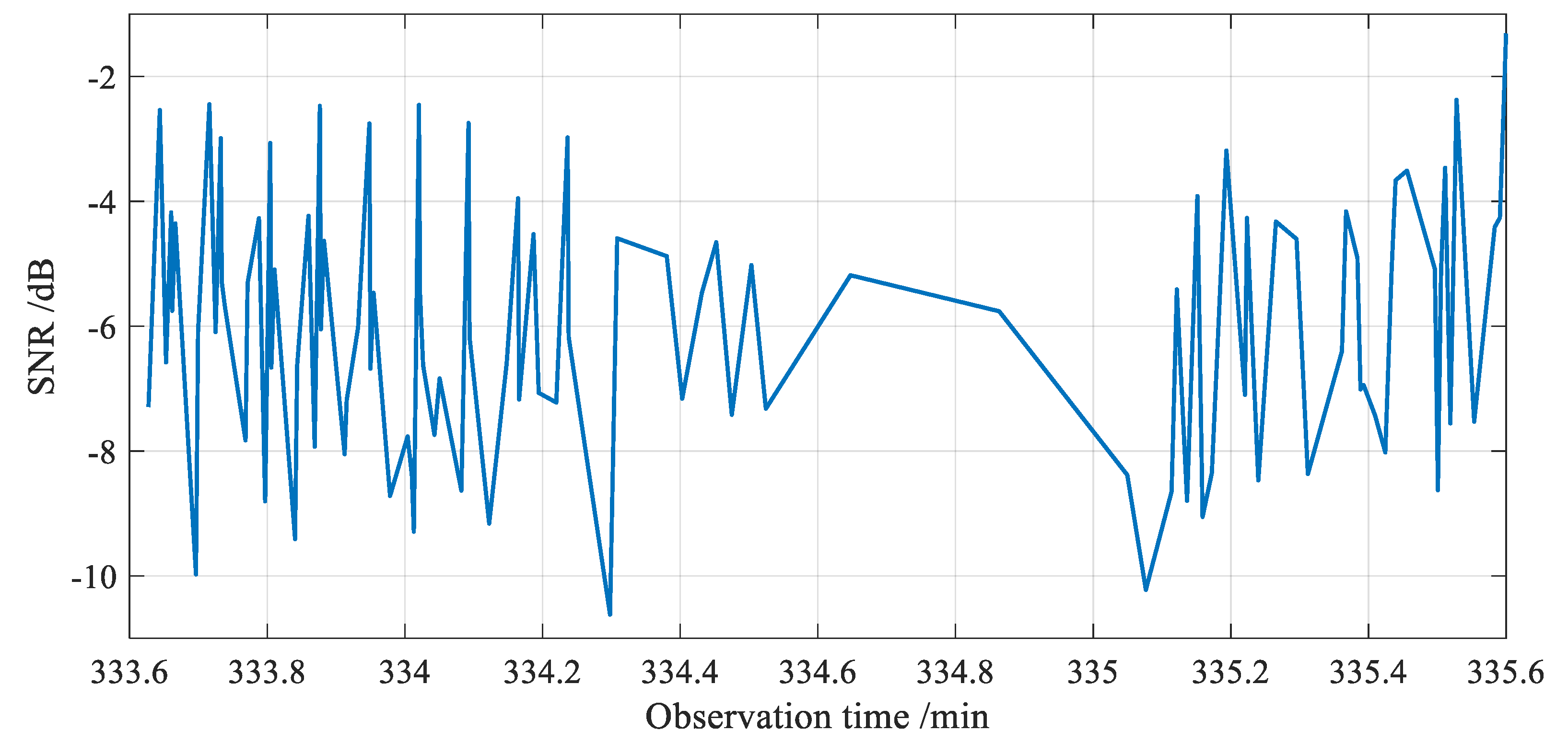
Variations in age, operational status, and orbital characteristics among individual Iridium satellites contribute to significant SNR fluctuations. Furthermore, Iridium’s beam-switching mechanism introduces sever SNR fluctuations even among epochs originating from the same satellite. Figure 3 presents empirical SNR measurements from 100 real Iridium signal epochs. The SNR fluctuation reaches about 9 dB during the 2 min observation window and demonstrates numerous instantaneous SNR transitions. These abrupt variations necessitate that positioning algorithms explicitly account for SNR effects and implement real-time adaptive adjustments.

2.3.2. The Variations in Doppler

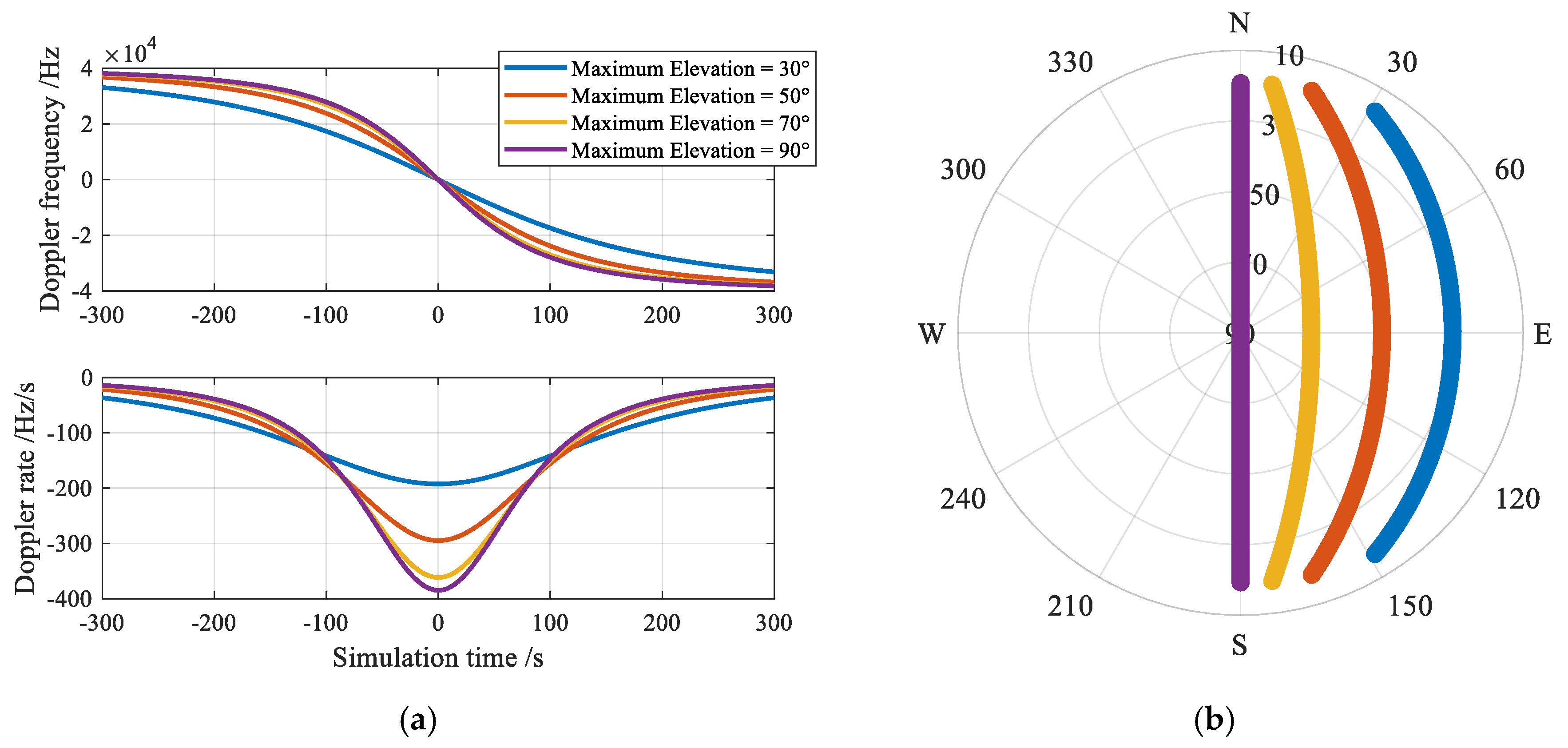
The high relative velocity between Iridium satellites and ground receivers generates significant Doppler frequency variations in the carrier of LEO signal. Figure 4 presents the simulated Doppler frequency and Doppler rate dynamics across three distinct Iridium orbital planes. The maximum Doppler frequency and Doppler rate values exhibit positive correlation with the satellite’s maximum elevation angle. During zenith passes (90° elevation), the absolute Doppler frequency approaches 40 kHz, while the maximum Doppler rate reaches 400 Hz/s. These extreme dynamics necessitate real-time parameter adaptation in positioning algorithms based on instantaneous Doppler characteristics.

3. The Agent-Weighted RLS Positioning Framework

This paper proposes an Agent-Weighted RLS Positioning Framework (AWR-PF) for LEO SOP positioning to achieve real-time epoch dynamic weight decision-making and establish temporal dependencies between epochs. The innovation lies in designing a neural network-based agent that comprehensively evaluates each epoch in real-time based on multiple characteristics (ephemeris age, elevation angle, azimuth angle, satellite-to-receiver distance, SNR, Doppler frequency, and epoch rank within its satellite). The agent additionally incorporates current observation matrix GDOP information. The evaluation result is expressed as a dynamically generated weight, which participates in RLS iteration to enhance positioning accuracy.
To train the agent, we formulated an MDP model including state, environment, action, reward, and state transition process. This MDP model integrates all Iridium epoch characteristics and iteratively updates based on selected action. Using the DDQN-EW algorithm, we trained the agent on an extensive real-world dataset comprising 107 h of continuous observations, ensuring full 24 h coverage and representative sampling of all characteristic Iridium signal conditions. The trained agent effectively learns epoch credibility evaluation across dynamic scenarios, enabling comprehensive and robust positioning accuracy optimization.
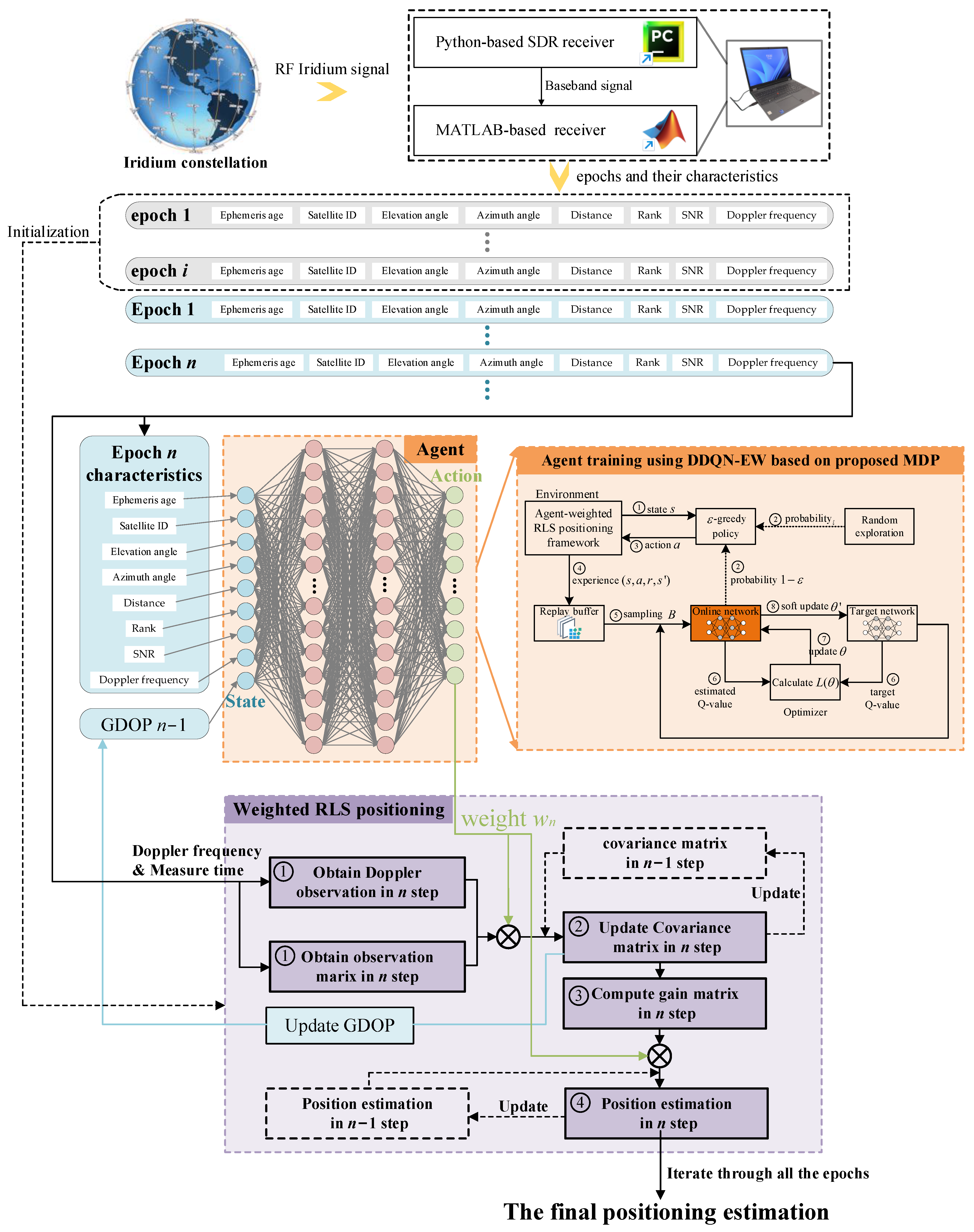
As demonstrated in Figure 5, the framework initially computes the preliminary position estimation, observation matrix, and covariance matrix using epochs accumulated during an initialization period. Then it performs epoch-wise recursive estimation, where an agent dynamically weights each n-th epoch based on its multi-dimensional features and current matrix conditions, and subsequently updates the position estimate and observation matrix through weighted RLS (Algorithm 1) until all epochs are processed to obtain the final position estimation.
Algorithm 1 Agent-Weighted RLS Positioning Framework
Input: Initial position, LEO satellite epochs.
Output: Recursive position estimation.
1//Initialize via LSM (LSM denotes least squares method):
2Construct observation equation G 0 . //Equations (11) and (12)
3Compute initial position estimation Δ x ^ 0 . //Equation (13)
4 Compute   initial   covariance   matrix   P 0 . //Equation (14)
5//Iterations:
6for each new epoch n  do
7         Obtain the weight w n through the agent.
8        Obtain new observation Δ Δ F n and observation matrix Δ G n .
9        //Update covariance matrix and GDOP.
10         P n = P n 1 P n 1 Δ G n T I 1 w n + Δ G n P n 1 Δ G n T 1 Δ G n P n 1 .
11         G D O P n = Trace P n .
12         //Compute gain matrix of this epoch.
13          K n = P n Δ G n T .
14         //Update position estimation.
15          Δ x ^ n = Δ x ^ n 1 + w n K n Δ G n T Δ Δ F n Δ G n Δ x ^ n 1 .
16end for
17return the final position estimation.
Before applying the RLS for position estimation, an initial position estimate is required. This is to ensure that the recursion starts with a reasonable initial state, allowing it to recursively update the target position as new observations become available. In this article, a small number of observations are first processed using the least squares method (LSM) to obtain an initial positioning result. Subsequently, as epochs are captured, the RLS algorithm is applied to perform recursive estimation of the observations. Using the epochs from the first t 0 time to establish the observation equation, assuming there are i 0 LEO satellites during this period and the i -th satellite has k i 0 Doppler observation epochs, the observation equation can be written as:
ρ ˙ u 1 ( 1 ) ρ ˙ u 1 ( k 1 0 ) ρ ˙ u i 0 ( 1 ) ρ ˙ u i 0 ( k i 0 0 ) ρ ˙ ˜ u 1 ( 1 ) ρ ˙ ˜ u 1 ( k 1 0 ) ρ ˙ ˜ u i 0 ( 1 ) ρ ˙ ˜ u i 0 ( k i 0 0 ) = ρ ˙ u 1 ( 1 ) x u ρ ˙ u 1 ( 1 ) y u ρ ˙ u 1 ( 1 ) z u c 0 ρ ˙ u 1 ( k 1 0 ) x u ρ ˙ u 1 ( k 1 0 ) y u ρ ˙ u 1 ( k 1 0 ) z u c 0 ρ ˙ u i 0 ( 1 ) x u ρ ˙ u i 0 ( 1 ) y u ρ ˙ u i 0 ( 1 ) z u 0 c ρ ˙ u i 0 ( k i 0 0 ) x u ρ ˙ u i 0 ( k i 0 0 ) y u ρ ˙ u i 0 ( k i 0 0 ) z u 0 c Δ x u Δ y u Δ z u Δ δ ˙ T 1 0 Δ δ ˙ T i 0 0 + ε
where ρ ˙ ˜ u i denotes the approximate value of the rate of change of the pseudorange after Taylor expansion; ρ ˙ u i / x u , ρ ˙ u i / y u , and ρ ˙ u i / z u are the partial derivatives of the pseudorange rate with respect to the three-dimensional position coordinates; and ε ~ N 0 , C ε denotes the joint Gaussian: white noise with covariance matrix C ε . For simplicity, Equation (11) can be written as:
Δ F 0 = G 0 Δ x 0 + ε
where Δ F 0 represents the initial observation vector, G 0 is the initial coefficient matrix, and Δ x 0 is the initial state vector. Using the minimum variance unbiased estimator (MVUE) for the linear equation, the estimation of Δ x 0 can be obtained as:
Δ x ^ 0 = ( G 0 T G 0 ) 1 G 0 T Δ F 0
Simultaneously, the covariance matrix of the initial state is given by:
P 0 = [ G 0 T G 0 ] 1
In this way, the initial state estimate Δ x ^ 0 and the initial covariance matrix P 0 are obtained, providing the foundation for subsequent recursive calculations.
After obtaining the initial state estimate, each time an epoch is captured, it is added to the equation for an iterative calculation. Suppose that at the (n − 1)-th iteration, the state estimate is Δ x ^ n 1 and the error covariance matrix is P n 1 . When a new n-th epoch is added, the agent determines the weight of the epoch based on the epoch characteristics and GDOP, which can be written as:
w n = A g e n t E A , I D Sat , A e , A a , S R D , R SatID , S N R , f d n , G D O P n 1
where E A denotes the ephemeris age, I D Sat denotes the identification of the Iridium satellite, A e denotes the elevation angle, A a denotes the azimuth angle, S R D denotes the satellite-to-receiver distance, R SatID denotes the epoch rank in the satellite, and f d denotes the estimated Doppler frequency. The new observation value of the epoch is Δ Δ F n and the new observation coefficient matrix is Δ G n , expressed as:
Δ Δ F n = ρ ˙ u ( n ) ρ ˙ ˜ u ( n ) Δ G n = ρ ˙ u ( n ) x u ρ ˙ u ( n ) y u ρ ˙ u ( n ) z u c 0
To obtain the near real-time position estimation, the RLS is employed, which allows for recursive updates of the parameter matrix and state estimate based on existing values, after adding new observations. First, the covariance matrix is updated recursively. When a new observation is added at the n-th step, the new covariance matrix, based on the covariance matrix from the (n − 1)-th step and the weight w n obtained by the agent, can be written as:
P n = P n 1 P n 1 Δ G n T I 1 w n + Δ G n P n 1 Δ G n T 1 Δ G n P n 1
where I denotes the identity matrix. Then the gain matrix for the n-th step is determined, which is used to balance the influence of the new observation on the state update and can be expressed as:
K n = P n Δ G n T
Finally, the weighted recursive update for the state estimate at the n-th step can be obtained as:
Δ x ^ n = Δ x ^ n 1 + w n K n Δ G n T Δ Δ F n Δ G n Δ x ^ n 1
By iteratively using Equations (17)–(19), the state estimate at each step can be recursively obtained, which corresponds to the 3D position solution of the receiver at each step.

4. Agent Training with Markov Decision Process (MDP)

In the AWR-PF proposed in Section 3, the time-varying epoch observation characteristics (SNR, Doppler frequency, azimuth angle, etc.) and the temporal dependencies of epoch-weighting decisions collectively constitute a complex sequential decision-making problem. The MDP model provides a mathematical foundation for the agent to comprehend the AWR-PF and formulate decisions by modeling the state evolution mechanisms, action influence pathways, and long-term reward quantification mechanisms. The model’s definitions of state space, action space, state transitions, and reward function directly determine the upper bound of the agent’s decision-making performance.
To efficiently solve for optimal policies in such high-dimensional continuous state spaces, we employ DDQN—a DRL algorithm that decouples action selection from value estimation to mitigate Q-value overestimation. This approach establishes a novel paradigm for addressing the dynamic epoch-weighting optimization challenges in LEO SOP positioning. The DDQN-based training framework enables the agent to learn a robust weighting policy while maintaining generalization performance in complex positioning scenarios.

4.1. Design of the MDP Model

In the AWR-PF, we formulate the agent’s observable state space by integrating multi-dimensional information extracted from four layers: satellite, epoch, signal, and positioning. The action space is systematically constrained within a scientifically determined weighting range to ensure operational validity. A dynamic reward mechanism is designed to precisely quantify positioning error variations, while the state transition process is meticulously designed to reflect system dynamics. This integrated approach yields a mathematically rigorous MDP model that enables comprehensive epoch validity assessment for optimal weighting decisions. The proposed model establishes a theoretical foundation for intelligent epoch-weight optimization in advanced LEO SOP positioning systems.

4.1.1. Definitions of Each Element in the MDP Model

Consider a continuous sequence of M epochs E n + 1 , E n + 2 , , E n + M from the actual collected epoch set E = E n n = 1 , 2 , , N as the weighting targets for a complete iterative positioning process, where M = M 1 + M 2 . The first M 1 epochs E n + 1 , E n + 2 , , E n + M 1 are used for initial positioning, while the weights of the subsequent M 2 epochs E n + M 1 + 1 , E n + M 1 + 2 , , E n + M 1 + M 2 are determined by the agent.
Next, we define that at each timestep t , the agent observes the environmental state and makes weighting decisions, completing one interaction with the environment (i.e., AWR-PF). After T timesteps, the final positioning result is obtained, where T = M 2 . We define the agent’s interaction with the environment over these T timesteps as an episode.
At any timestep t , the agent’s decision-making process for the weight of epoch E n can be represented by the MDP model as a tuple S ( t ) , A ( t ) , R ( t ) , S ( t ) . The following will introduce each element of the tuple in detail.
At timestep t , the state S ( t ) observed by the agent from the environment is represented as S ( t ) = S satellite ( t ) , S epoch ( t ) , S signal ( t ) , S GDOP ( t ) , with a state space dimension of 9 (comprising 9 components). S ( t ) denotes the next state transitioned to after the agent observes S ( t ) and takes action A ( t ) , expressed as S ( t ) = S ( t + 1 ) .
The satellite state S satellite ( t ) observed by the agent at timestep t is defined as:
S satellite ( t ) = S age ( t ) , S azimuth ( t ) , S elevation ( t ) , S distance ( t )
where S age ( t ) denotes the ephemeris age (corresponding to E A in Equation (15)) derived from the observed ephemeris data, S azimuth ( t ) denotes the azimuth angle (corresponding to A a in Equation (15)) of the satellite associated with epoch E n , S elevation ( t ) denotes the elevation angle (corresponding to A e in Equation (15)) of the same satellite, and S distance ( t ) denotes the satellite-to-receiver distance (corresponding to S R D in Equation (15)). These components collectively characterize the satellite state for the agent’s positioning decisions.
The epoch state S epoch ( t ) observed by the agent at timestep t is defined as:
S epoch ( t ) = S id ( t ) , S rank ( t )
where S id ( t ) denotes the satellite identifier (corresponding to I D Sat in Equation (15)) associated with epoch E n , and S rank ( t ) denotes the cumulative observation count (corresponding to R SatID in Equation (15)) of the corresponding satellite from the initial timestep up to the current timestep t . This provides essential epoch identification and historical tracking information for the agent.
The signal state S signal ( t ) observed by the agent at timestep t is defined as:
S signal ( t ) = S snr ( t ) , S Doppler ( t )
where S snr ( t ) denotes the SNR (corresponding to S N R in Equation (15)) of the observed epoch E n , and S Doppler ( t ) denotes the Doppler frequency (corresponding to f d in Equation (15)) of the corresponding signal. These measurements provide critical signal quality metrics for the agent’s weighting decisions.
Additionally, S GDOP ( t ) denotes the latest GDOP value (corresponding to G D O P n 1 in Equation (15)) obtained by the agent at timestep t through the weighted RLS algorithm, which serves as the agent’s observation of the current positioning system state.
At timestep t , the weight action A ( t ) (corresponding to w n in Equation (15)) is determined by the agent after observing state S ( t ) through epoch E n , with a discrete action space defined as A ( t ) { 0.1 , 0.2 , , 2 } containing 20 possible weight values. The agent evaluates each component of the current state S ( t ) to assess epoch quality, quantizes this evaluation into a discrete weight value, and subsequently applies the selected weight to the weighted RLS algorithm to perform an iterative positioning update incorporating the current epoch’s information.
The reward function R ( t ) is designed to evaluate the agent’s weighting decision A ( t ) during the state transition from S ( t ) to S ( t ) , which can be formulated as:
R ( t ) = k 1 ( e ( t 1 ) e ( t ) ) + k 2 e ( t 1 ) e ( t ) e ( t 1 ) + σ
where e ( t ) denotes the positioning error obtained by comparing the AWR-PF output with the true position at timestep t , and e ( 0 ) denotes the initial positioning error. The minimum offset term σ is utilized to prevent the problem of an infinitely large reward due to e ( t 1 ) becoming exactly zero or near zero. The reward coefficients k 1 and k 2 serve distinct purposes: k 1 focuses on absolute error reduction to encourage a rapid initial error decrease, while k 2 emphasizes relative error reduction (percentage change) to promote stable convergence during later positioning stages, collectively guiding the agent’s learning toward both immediate and long-term positioning accuracy improvements during training.
Our research aims to determine optimal epoch weights to minimize positioning errors. The optimization objective is defined as maximizing the expected discounted cumulative reward:
V = max θ E t = 1 T γ t 1 R ( t ) θ
where θ denotes the parameters of the agent’s neural network, and γ ( 0 , 1 ] denotes the discount factor that balances the importance between immediate and long-term rewards. This formulation effectively models the trade-off between rapid error reduction in early iterations and sustained accuracy improvement throughout the positioning process.

4.1.2. Analysis of the MDP Model Based on the Dynamic Bayesian Network

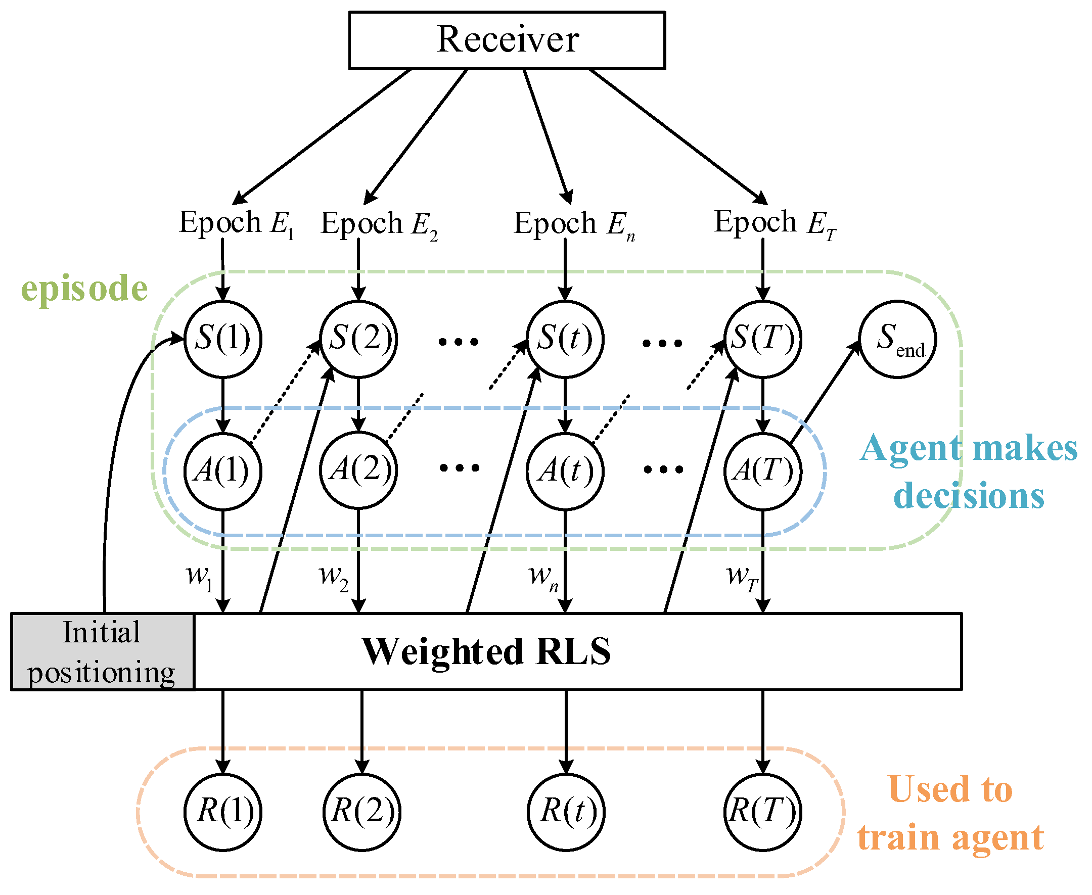
To further analyze this MDP model, Figure 6 illustrates the corresponding dynamic Bayesian network (DBN) model that visually captures the temporal dependency relationships between states, actions, and rewards during the positioning process. This figure explicitly shows how the agent’s weighting decisions A ( t ) at each timestep influence both the immediate reward R ( t ) and the state transition S ( t ) S ( t ) , while maintaining the Markov property where each state depends on its immediate predecessor. The DBN structure particularly highlights the sequential nature of the proposed AWR-PF, where epoch-specific observations progressively refine the positioning solution through the agent’s learned weighting policy.
The MDP’s state transition mechanism can be comprehensively illustrated through the example of S ( 1 ) , A ( 1 ) , R ( 1 ) , S ( 1 ) . The agent initially constructs the complete state S ( 1 ) by integrating: (1) S signal ( 1 ) , which includes SNR and Doppler frequency from the first epoch; (2) S epoch ( 1 ) , containing the satellite identifier and cumulative observation count; (3) S satellite ( 1 ) , comprising ephemeris age, azimuth/elevation angles, and satellite–receiver distance; and (4) S GDOP ( 1 ) , obtained from the covariance matrix.
Upon receiving S ( 1 ) , the agent generates weighting decision A ( 1 ) , which is applied in the weighted RLS positioning. The resulting position estimate yields positioning error e ( 1 ) through comparison with the true position, enabling reward computation R ( 1 ) , which combines both absolute ( k 1 -weighted) and relative ( k 2 -weighted) error improvements from the initial error e ( 0 ) . Then the agent utilizes R ( 1 ) to optimize its parameters. The subsequent state S ( 1 ) (equivalent to S ( 2 ) ) is then assembled from the second epoch’s corresponding measurements, maintaining the temporal progression of the positioning process.
This transition logic iterates sequentially until terminal conditions are met. At the final timestep T , after determining A ( T ) and computing R ( T ) , the system enters termination state S end —a null state indicating episode completion when all epoch weights have been decided. The complete cycle demonstrates how the MDP model achieves progressive positioning optimization through intelligent epoch weighting.

4.2. DRL-Based Solution

To address the sequential decision-making challenge in epoch weighting, we have established the MDP model as detailed in Section 3. Given the complexity of the multi-level state space S ( t ) and the discrete nature of action space A ( t ) while pursuing long-term cumulative reward maximization, we employ DRL for optimal policy derivation.
While conventional value-based deep reinforcement learning approaches like the Deep Q-Network (DQN) [29] offer theoretically sound solutions for Markov decision processes, they exhibit significant limitations when applied to the complex state–action spaces characteristic of our epoch weighting problem. The algorithm’s well-documented propensity for Q-value overestimation [30] originates from its fundamental architecture—specifically, the use of a single network to perform dual functions: both selecting the optimal action and evaluating its value. To mitigate the Q-value overestimation issue inherent in the DQN algorithm and enhance both the stability of the learning process and the performance of the final policy, we adopt the DDQN algorithm.
The key improvement of DDQN lies in its decoupling of action selection and value estimation in the target Q-value computation, achieved through the use of an online network and a target network. Specifically, the online network Q ( s , a ; θ ) (with parameters θ ), which undergoes continuous updates and is responsible for action exploration and selection based on current knowledge, determines the optimal action: a = arg max a Q ( s , a ; θ ) , where s denotes the current state, a denotes the currently determined selected action, s denotes the next state, and a denotes the set of admissible actions available at state s . The value of the selected action is then evaluated by the target network Q ( s , a ; θ ) (with parameters θ ), which periodically synchronizes its parameters from the online network to provide a relatively stable benchmark for value estimation: Q ( s , a ; θ ) . This decoupling mechanism effectively mitigates the Q-value overestimation problem.
While DDQN is conventionally applied in video game domains—where raw pixel frames serve as sequential input states processed through convolutional neural networks (CNNs) for feature extraction and direct-action generation (e.g., movement controls), with rewards derived from game scores to enable end-to-end learning—their direct adaptation to satellite navigation presents fundamental challenges. In LEO SOP applications, raw signal waveform images are unintelligible to agents without engineered state representations. Direct positioning output would cause exponential action space expansion, while undefined reward mechanisms for navigation problems require careful design.
To address these limitations, we innovatively customize DDQN:
  • Structured State Representation: Extracting positioning-relevant features from satellite, epoch, signal, and positioning layers using lightweight neural networks, enabling efficient interpretation of mathematical relationships.
  • Collaborative Decision Framework: Integrating the agent with RLS within the AWR-PF, where the agent evaluates epoch credibility and outputs weight for RLS-based positioning, dramatically reducing decision complexity.
  • Differential Reward Mechanism: Incorporating both absolute and proportional positioning error changes—rather than instantaneous error alone—to account for convergence dynamics during iterative positioning.
These adaptations transform DDQN from a gaming solution into a viable satellite positioning optimizer: the DDQN-based Epoch Weighting (DDQN-EW) algorithm. Subsequently, we will detail DDQN-EW’s implementation.

4.2.1. Network Architecture

Given that the state S ( t ) in our proposed MDP model comprises nine key environmental parameters (including a four-dimensional satellite state: ephemeris age, azimuth angle, elevation angle, and satellite-ground distance; two-dimensional epoch state: satellite identifier and cumulative observation count; two-dimensional signal state: SNR and Doppler frequency; and one-dimensional positioning state: GDOP), we represent it as a nine-dimensional feature vector.
We employ a multi-layer perceptron (MLP) as the approximator for the Q-value function, with identical architectures for both the online network and target network. Below, we define the structure of this MLP.
First, the input layer consists of nine neurons, matching the dimensionality of the state vector. Next, the network includes two hidden layers: the first is a fully connected (FC) layer with H 1 neurons, activated by the rectified linear unit (ReLU), and the second is another FC layer with H 2 neurons, also using ReLU activation. Finally, the output layer is an FC layer with 20 neurons, each corresponding to a discrete action, and if no activation function is applied, it allows direct Q-value estimation.
In evaluation mode, the agent selects the action associated with the highest Q-value in the output layer. In training mode, the agent adopts the ε greedy policy (see Section 4.2.3 for details) to determine actions.

4.2.2. Optimization Objective

The optimization objective of the online network is to minimize the discrepancy between its predicted Q-value Q ( s , a ; θ ) and the target Q-values computed by the target network:
y = r + γ ( 1 d ) Q ( s , arg max a Q ( s , a ; θ ) ; θ )
where d denotes the terminal state indicator (1 if s is terminal state, 0 otherwise). We employ the mean squared error (MSE) as the loss function:
L ( θ ) = E ( s , a , r , s , d ) B ( y Q ( s , a ; θ ) ) 2
The online network parameters θ are updated using the adaptive moment estimation (Adam) optimizer, which computes gradients based on L ( θ ) . The learning rate (denoted as α ) stands as the most critical hyperparameter in the Adam optimizer. This fundamental parameter governs the step size for updating neural network parameters during the optimization process, while the optimizer itself determines the parameter updates based on both L ( θ ) and α . The way the optimizer updates the network parameters is θ θ α θ L ( θ ) , where θ L ( θ ) denotes the gradient of L ( θ ) with respect to θ .

4.2.3. Efficient Training Mechanism

To break the temporal correlation between data samples and improve sample utilization, we incorporate experience replay. Each interaction between the agent and the environment generates an experience tuple s , a , r , s , d , which is stored in a fixed-size replay buffer D . Here, r denotes the immediate reward following the state transition from s to s via action a . The buffer operates as a first-in-first-out (FIFO) queue with a maximum capacity of N D . During training iterations, a mini-batch of N B experience tuples is uniformly sampled at random from the replay buffer:
B = { ( s i , a i , r i , s i , d i ) } i = 1 , 2 , , N b
which is then used to compute the loss function and update the online network.
To provide stable learning targets, we maintain a separate target network Q ( s , a ; θ ) . Unlike the online network Q ( s , a ; θ ) , the target network’s parameters θ are not updated via gradient descent but instead through a soft update mechanism: after each update of the online network parameters θ , the target network parameters are adjusted as follows:
θ τ θ + ( 1 τ ) θ
where τ is the update rate, controlling the speed at which the target network parameters converge toward those of the online network.
To balance exploration of new actions and exploitation of current knowledge during training, we employ the ε greedy policy as the behavior strategy for action selection. With probability ε , an action is chosen uniformly at random from the action space A ( t ) ; with probability 1 ε , the agent selects the current optimal action corresponding to the highest Q-value output by the online network. The exploration rate ε decays over time according to:
ε = max ( ε min , λ ε )
where ε min is the minimum exploration rate, λ is the decay rate, and ε is initialized to 1. This ensures that the policy prioritizes exploration in early training stages and gradually shifts toward exploitation as learning progresses.

4.2.4. Once Training Process

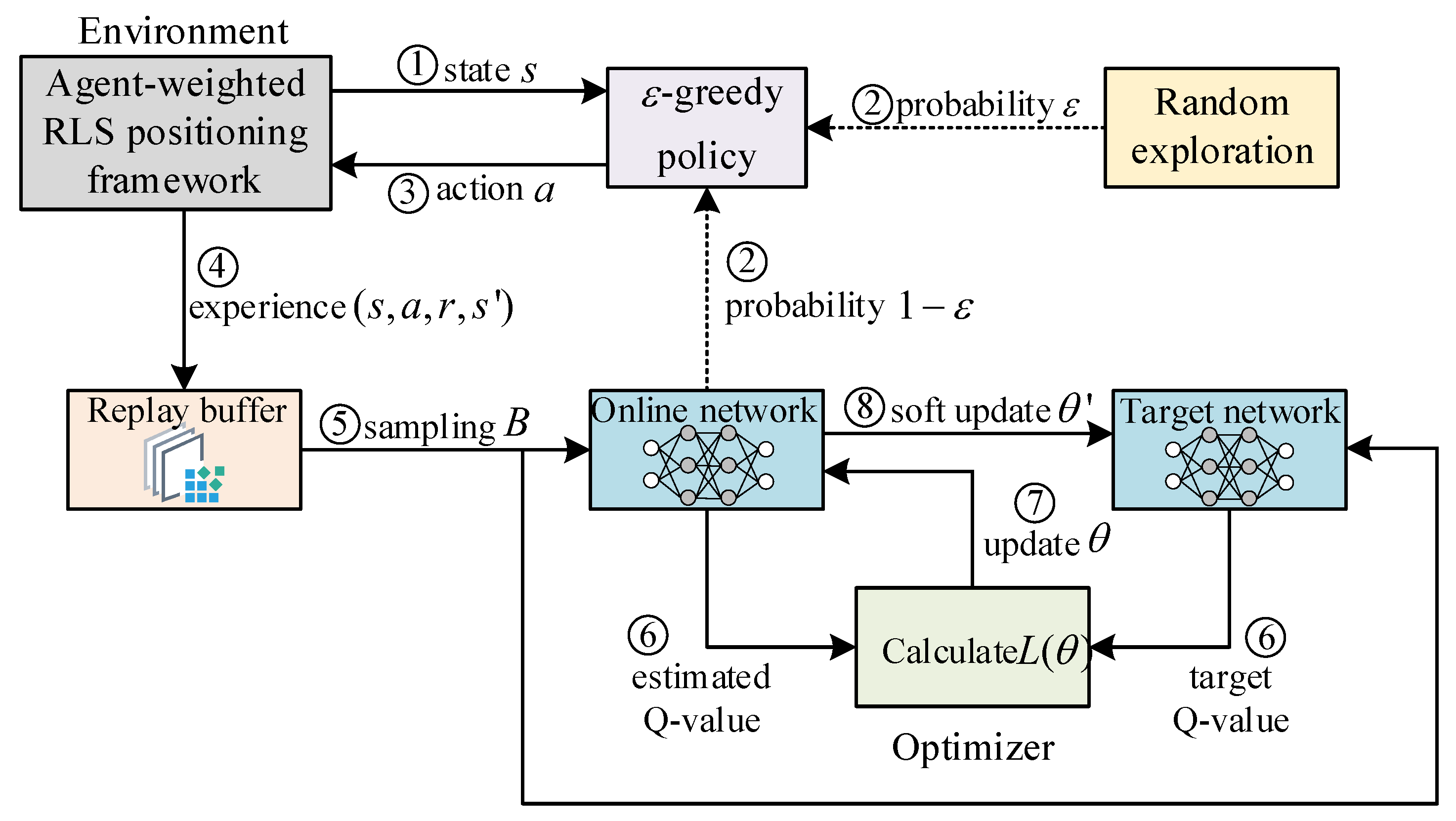
The single training process of the DDQN-EW agent is illustrated in Figure 7. The process begins with the agent observing the current state s from the AWR-PF. An action a is then selected according to the ε greedy policy. Upon executing action a , the weight for the current epoch is determined, and the weighted RLS algorithm performs a single iterative positioning update using this weight combined with epoch-specific information. The positioning result is compared with the true position to compute the immediate reward r . The next state s is then observed, and the terminal flag d is determined based on s . The experience tuple s , a , r , s , d generated from this interaction is stored in the replay buffer D .
During training, a mini-batch B is sampled uniformly from the replay buffer D . The online network and target network are then used to compute the estimated Q-values and target Q-values, respectively. The optimizer calculates the loss L ( θ ) based on these values and performs backpropagation to update the online network parameters θ . Finally, the target network parameters θ are softly updated to complete one training iteration.
This iterative process ensures stable and efficient learning through the ε greedy policy, soft update, and experience replay mechanism.

4.2.5. Overall Training and Evaluation Process

The collected epoch set E is partitioned into subsets of length M , yielding N / M epoch subsets. For each subset, the first M 1 epochs are used for initial positioning, while the remaining epochs form an episode of length M 2 for training the agent (see Algorithm 2). This structured approach maximizes sample utilization efficiency and learning frequency while ensuring stable and uniform training progression. By optimizing both the injection and utilization processes of the experience replay buffer, it enables the learning process to closely follow the pace of agent–environment interactions.
Algorithm 2 Training Iteration of the DDQN-EW Algorithm
Input: Online network Q ( s , a ; θ ) , target network Q ( s , a ; θ ) , replay buffer D , exploration rate ε .
Output: The updated parameters θ and θ .
1for timestep t 1 , T  do
2    for episode k 1 , N / M  do
3        Agent observes state s k ( t ) from AWR-PF.
4        If  t 1  then
5             s k ( t 1 ) = s k ( t ) .
6        end if
7         d k ( t ) = 0 .
8        If  t = T  then
9             s k ( t ) = zeros ( 9 ) , d k ( t ) = 1 .
10        end if
11        With probability ε , agent randomly select an action from A ( t )   as   a k ( t ) ,
12        otherwise a k ( t ) = argmax i Q ( s k ( t ) , a i ; θ ) .
13         ε = max ( ε min , λ ε ) .
14        Obtain reward r k ( t ) from AWR-PF.
15        Store tuple s k ( t ) , a k ( t ) , r k ( t ) , s k ( t ) , d k ( t ) in D .
16        Sample random mini-batch B form D .
17        Calculate estimated Q-value: y = r + γ ( 1 d ) Q ( s , arg max a Q ( s , a ; θ ) ; θ ) .
18        Calculate L ( θ ) = E ( s , a , r , s ) B ( y Q ( s , a ; θ ) ) 2 .
19        Update online network: θ θ α θ L ( θ ) .
20        Update target network: θ τ θ + ( 1 τ ) θ .
21    end for
22end for
Upon completion of agent training, we evaluate its generalization capability using a separately collected epoch set E = E n n = 1 , 2 , , N . Following the same protocol as the training phase, we partition E into N / M independent evaluation episodes. The trained agent then executes a pure exploitation policy (see Algorithm 3) to perform epoch-specific weighting and positioning throughout these episodes.
Algorithm 3 Evaluation Process of the Trained Agent
Input: Trained online network Q ( s , a ; θ ) .
1for timestep t 1 , T  do
2    for episode k 1 , N / M  do
3        Agent observes state s k ( t ) from AWR-PF.
4         a k ( t ) = argmax i Q ( s k ( t ) , a i ; θ ) .
5    end for
6end for

5. Experimental Results

5.1. Iridium Signal Data Acquisition

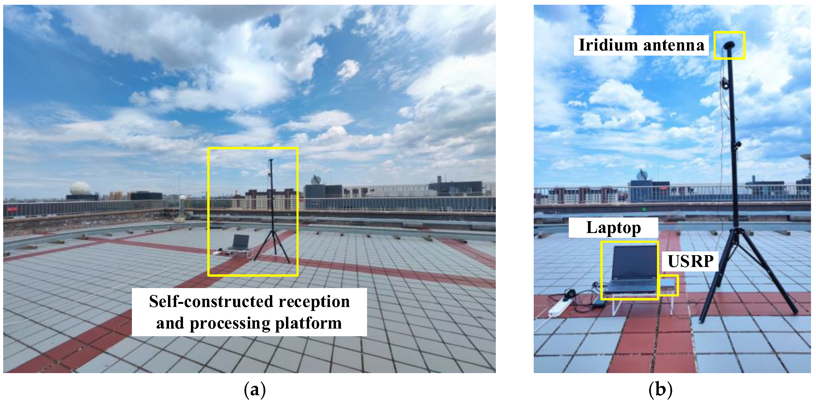
All real Iridium signal data collection was conducted at the Advance Technology Base of the Chinese Academy of Sciences in Beijing, China (40°04′15.45″E, 116°16′28.33″N, 90 m altitude), using a self-constructed reception and processing platform for Iridium signals. The platform was stationary and mounted on the rooftop to minimize signal characteristic variations caused by building obstructions (Figure 8a). As shown in Figure 8b, the platform comprises an Iridium antenna (JCYX008; Zhejiang JC Antenna Co., Ltd., Jiaxing, China), a universal software radio peripheral (USRP B210, Ettus Research, Austin, TX, USA), and a laptop computer (Lenovo ThinkPad X1). The platform enables the acquisition of Iridium signals and the extraction of epoch characteristics for subsequent applications including training and positioning trials.
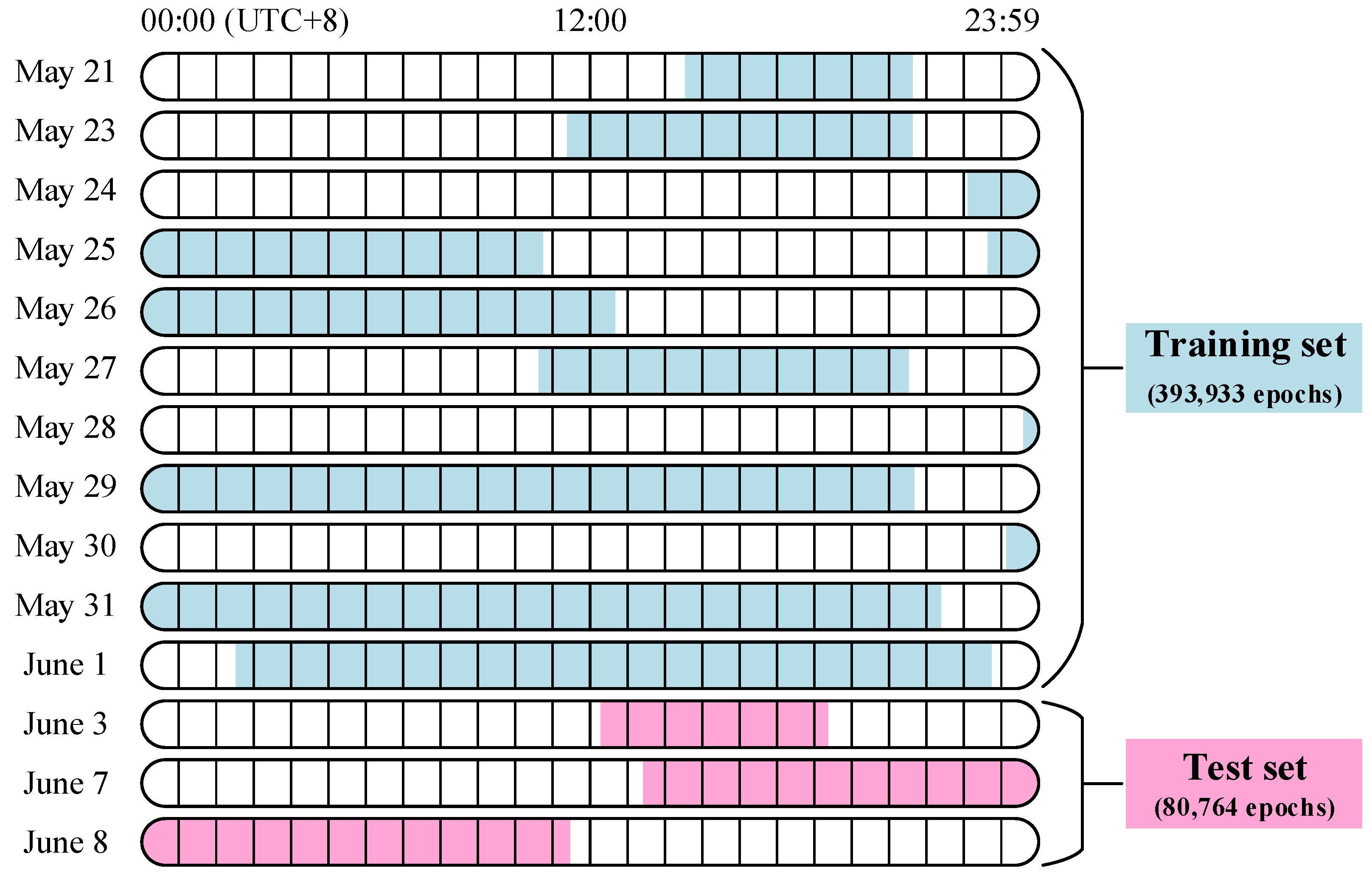
Through long-term observation of Iridium signals, we extracted 393,933 epochs with their characteristics from 107 h of real Iridium signal data to construct a 24 h-coverage training set. Additionally, we extracted 80,764 epochs from 28 h of real Iridium signal data to establish a test set for algorithm validation. The specific signal reception windows are illustrated in Figure 9.
During the reception of training set signals, we deliberately selected diverse observable windows to ensure epoch characteristic variability, thereby enhancing the generalization capability of the trained agent. For the test set, the signals covered nearly all 24 h of the day, enabling comprehensive evaluation of the agent’s positioning performance across all time periods.
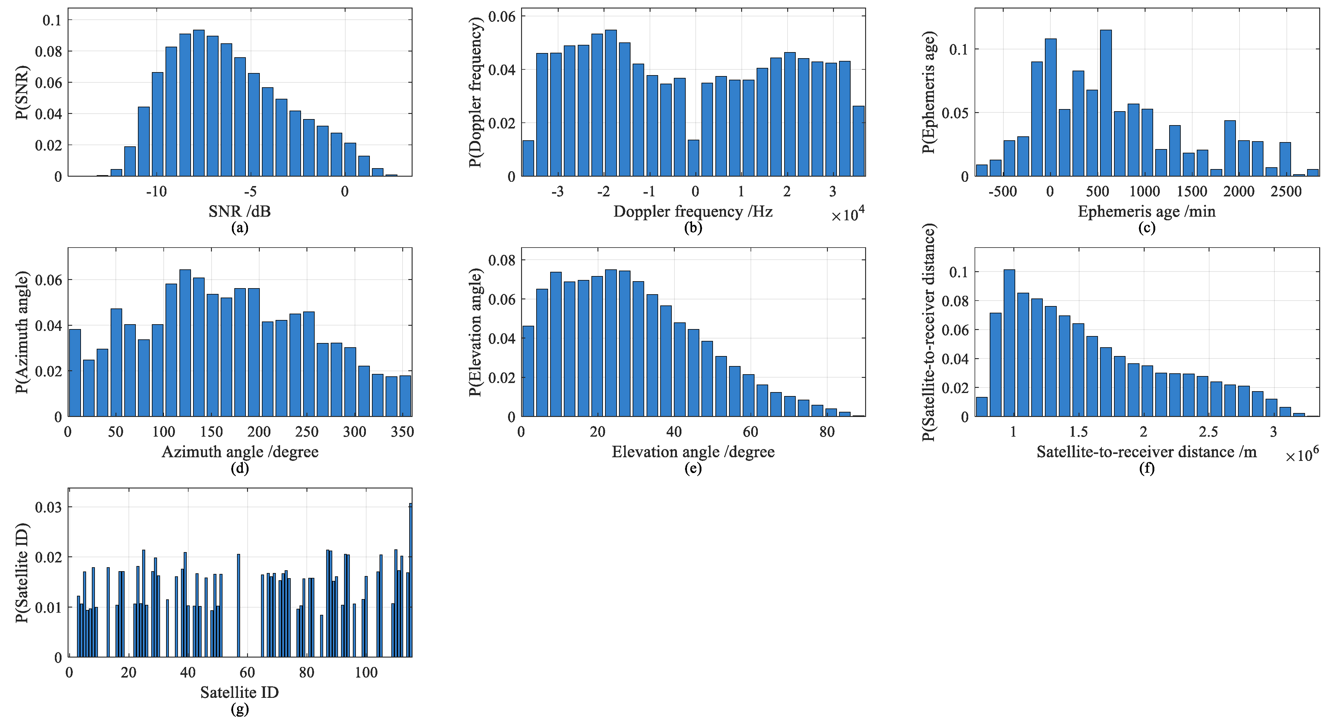
Figure 10 demonstrates that the captured Iridium epochs exhibited wide-ranging characteristic distributions: SNR spanned −14 dB to 4 dB, elevation angles covered 0° to 90°, and signals from 69 distinct satellites were acquired. These statistics confirm the training set’s comprehensive representation of Iridium epoch characteristics across diverse operational conditions, thereby enhancing the trained agent’s generalization capability and robustness when processing heterogeneous epoch samples.

5.2. Training Setup and Results

In this study, we employed a high-performance desktop computing system to train our agent after collecting a substantial volume of epoch signals. The experimental setup utilized an AMD Ryzen 9 9950X 16-core processor (Advanced Micro Devices, Inc.; Sunnyvale, CA, USA) with 48 GB RAM and an NVIDIA GeForce RTX 5070 Ti GPU (NVIDIA Corporation; Santa Clara, CA, USA), providing the necessary computational power for efficient DRL implementation. This hardware configuration enabled effective processing of the extensive navigation epoch data while supporting the computationally intensive training of our DDQN-based positioning system. The complete specifications of training hyperparameters, including batch sizes, learning rates, and network architectures, are systematically documented in Table 2 to ensure experimental reproducibility and facilitate comparative research in the field of navigation-oriented DRL.
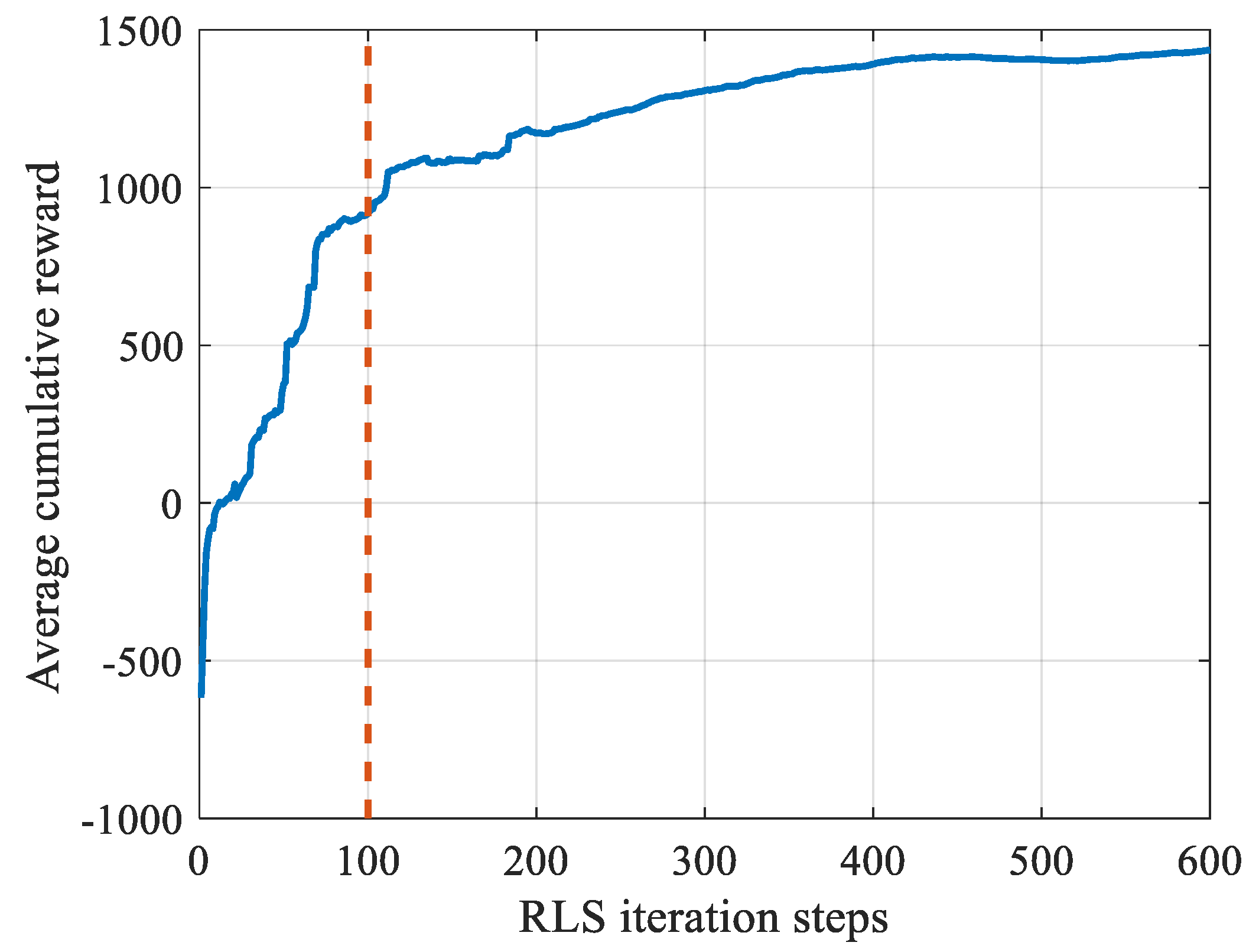
During the training of the agent, we recorded the average cumulative reward obtained during its interaction with the environment (as shown in Figure 11) to evaluate the learning performance. The average reward at each timestep is obtained by averaging the immediate rewards that the agent receives through environmental interactions at that specific timestep across multiple episodes. The cumulative average reward at the current timestep is then calculated by summing these average rewards from the initial timestep up to the present timestep. In the early training phase (from the initial timestep to the 100th timestep), the agent was in the exploration stage and predominantly made random decisions by outputting random weights. However, despite the large initial position estimation errors during the recursive initialization phase, the incorporation of epochs still led to a reduction in positioning errors, resulting in a rapid increase in the agent’s average cumulative reward by nearly 1500. Subsequently, as the agent gradually shifted toward exploitation mode and began making reasonable decisions based on acquired knowledge, the average cumulative reward slowly increased from approximately 900 to nearly 1400.
Furthermore, we introduced both “default” and “random” strategies to benchmark the performance of the agent during the training phase (as illustrated in Figure 12). The “default” strategy assigns a fixed weight of 1 to all epochs (i.e., standard RLS), while the “random” strategy uniformly samples a weight from the discrete set { 0.1 , 0.2 , , 2.0 } at each iteration. Observations revealed that the 3D positioning errors of all three approaches exhibited a consistent downward trend throughout the training process, which aligns with the fundamental principles of epoch-based positioning.
In the initial training phase, the agent predominantly output random weights with occasional selections of actions corresponding to the maximum Q-value. However, since DDQN-EW critically relies on stable value targets provided by the target network—whose parameters at this stage are derived from extremely limited and thus highly inaccurate data—the agent’s autonomous decisions were statistically suboptimal. Consequently, its positioning performance initially underperformed both the “default” and “random” strategies.
As training progresses, the agent continuously learns from batched experiences sampled from the replay buffer, progressively improving the accuracy of the target network’s Q-value estimations. This enables the agent to determine contextually appropriate weights based on varying epoch states, ultimately surpassing the “random” strategy in positioning accuracy. Nevertheless, likely due to convergence to a local optimum during network training, the agent’s final positioning performance eventually plateaued at a level comparable to that of the “default” strategy. Incorporating more epochs could enhance the agent’s positioning performance but risks overfitting to specific epoch characteristics. To ensure generalization, we deliberately limited training iterations. This constraint maintains robust performance across diverse scenarios while preventing over-specialization.

5.3. Evaluation Results

To validate the effectiveness of the proposed Agent-Weighted RLS Positioning Framework (AWR-PF), we conducted 97 independent positioning experiments using 28 h of real Iridium signal data. The intelligent agent in AWR-PF was the same as the one trained in Section 5.2. For comparative analysis, we selected two baseline algorithms: standard RLS (unweighted) and randomly weighted RLS (RWR), of which the weights sampled uniformly from (0, 2].
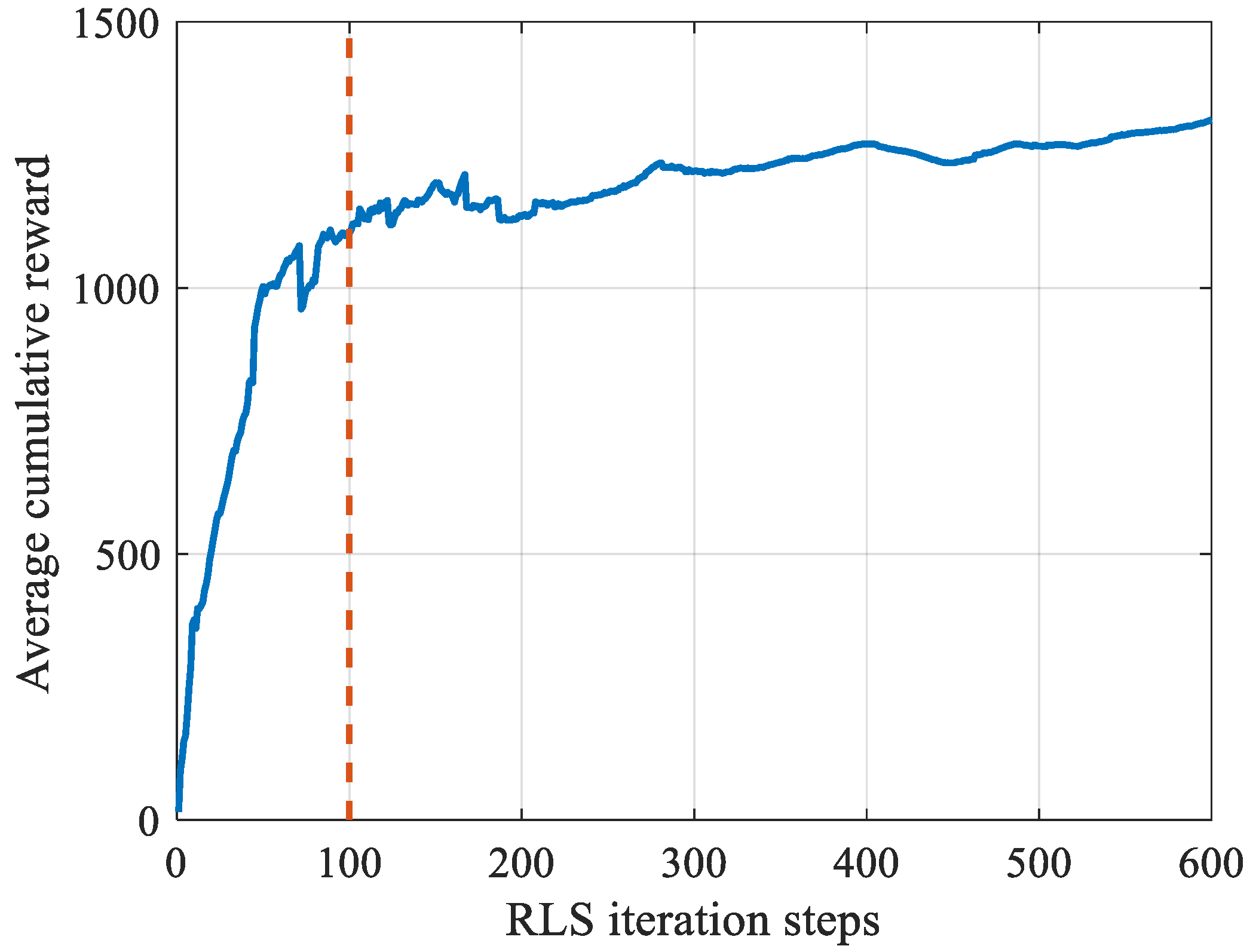
The average cumulative reward obtained by the agent in the test set was recorded (as shown in Figure 13). In the initial testing phase, when encountering states not sufficiently covered during training, the agent demonstrated remarkable robustness, achieving a high average cumulative reward of 1100. This indicates that the agent successfully learned an appropriate weight-determination strategy through DDQN-EW. Subsequently, the accumulated average reward gradually increased to 1300, which is slightly lower than the final average cumulative reward attained during the training phase.
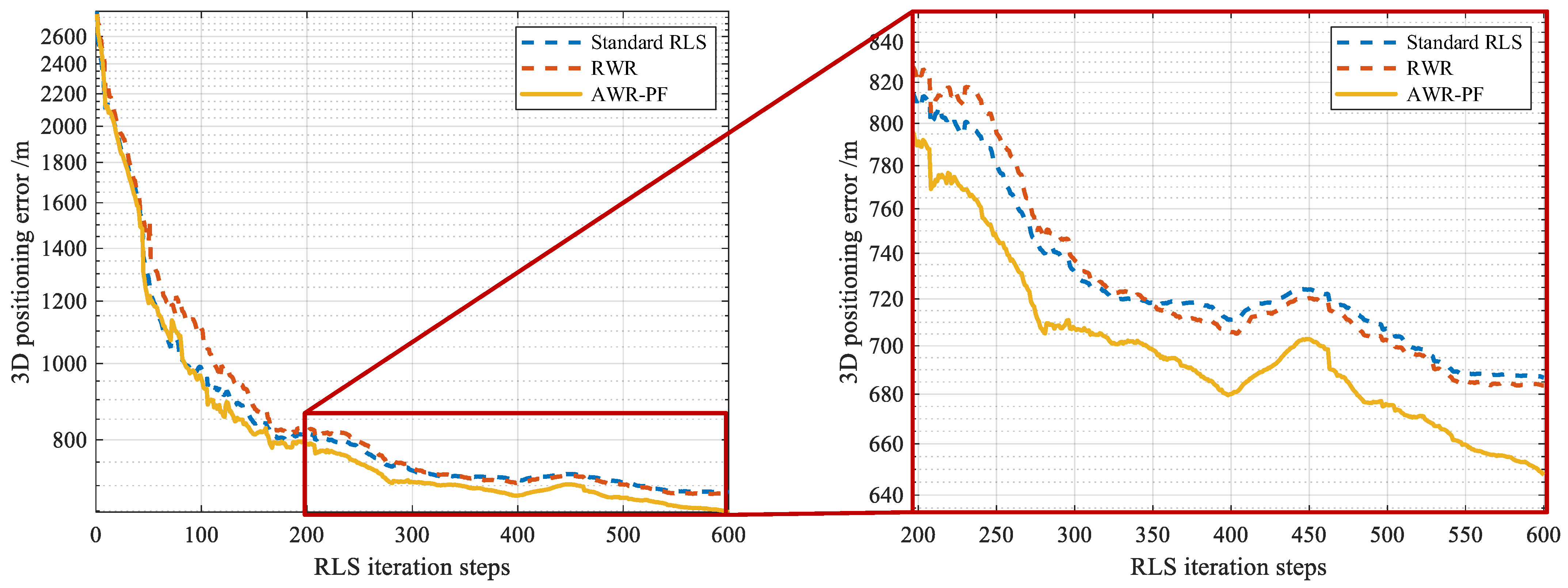
We compared the mean positioning accuracy of each step of the AWR-PF against both the standard RLS and RWR (Figure 14). Consistent with observations during training, all three approaches exhibited a sustained downward trend in 3D positioning error throughout the testing process. During the testing phase, the agent relies solely on acquired knowledge for autonomous decision-making without further exploration. This eliminates the need to recover from inaccurate initial positioning estimates caused by exploratory actions, resulting in significantly faster convergence of positioning errors compared to the training phase. During the initial testing steps, the agent immediately outperformed the RWR and approached the performance level of the standard RLS. This indicates that the trained agent successfully generalized knowledge acquired during training to the test set. As epoch weight determination progressed, the agent—benefiting from DDQN-EW’s characteristic bias toward robust decision-making—demonstrated increasingly stable performance. Consequently, AWR-PF consistently outperformed both the standard RLS and RWR in subsequent iterations.
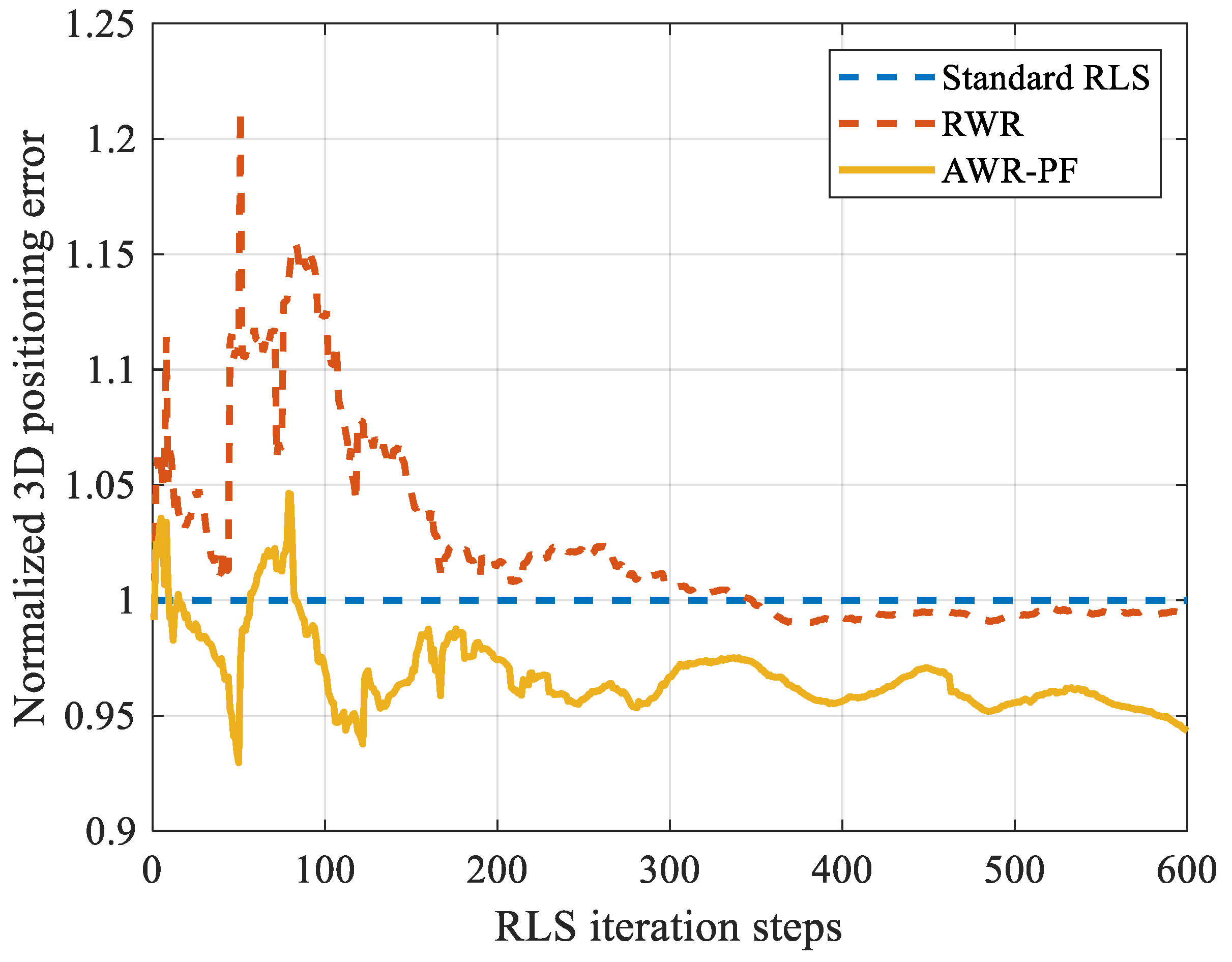
To exclude the influence of absolute positioning error variations across iterations, we calculated the relative positioning errors of both the AWR-PF and RWR with respect to the standard RLS. Using the standard RLS as the baseline, we normalized the positioning errors at each timestep, enabling direct visual comparison of the three methods’ performance throughout the iterative process (Figure 15). The results demonstrate that the RWR exhibited significant performance fluctuations in the initial phase, eventually converging to nearly identical performance with the standard RLS as iterations progressed. This convergence indicates the RWR’s inability to substantially reduce the positioning error with the iterations. In contrast to the RWR, while the proposed AWR-PF still showed some initial performance fluctuations, these variations were markedly smoother and consistently superior to those of the RWR approach. After approximately 100 iterations, the AWR-PF achieved a stable 5% average reduction in positioning error compared to the standard RLS. This performance advantage was maintained consistently throughout the remaining iterations. Notably, this accuracy improvement was derived from the average results of 97 independent positioning trials, conclusively demonstrating that the proposed AWR-PF fundamentally addressed the core optimization challenge of epoch-characteristic-based weighting, rather than achieving incidental performance gains.
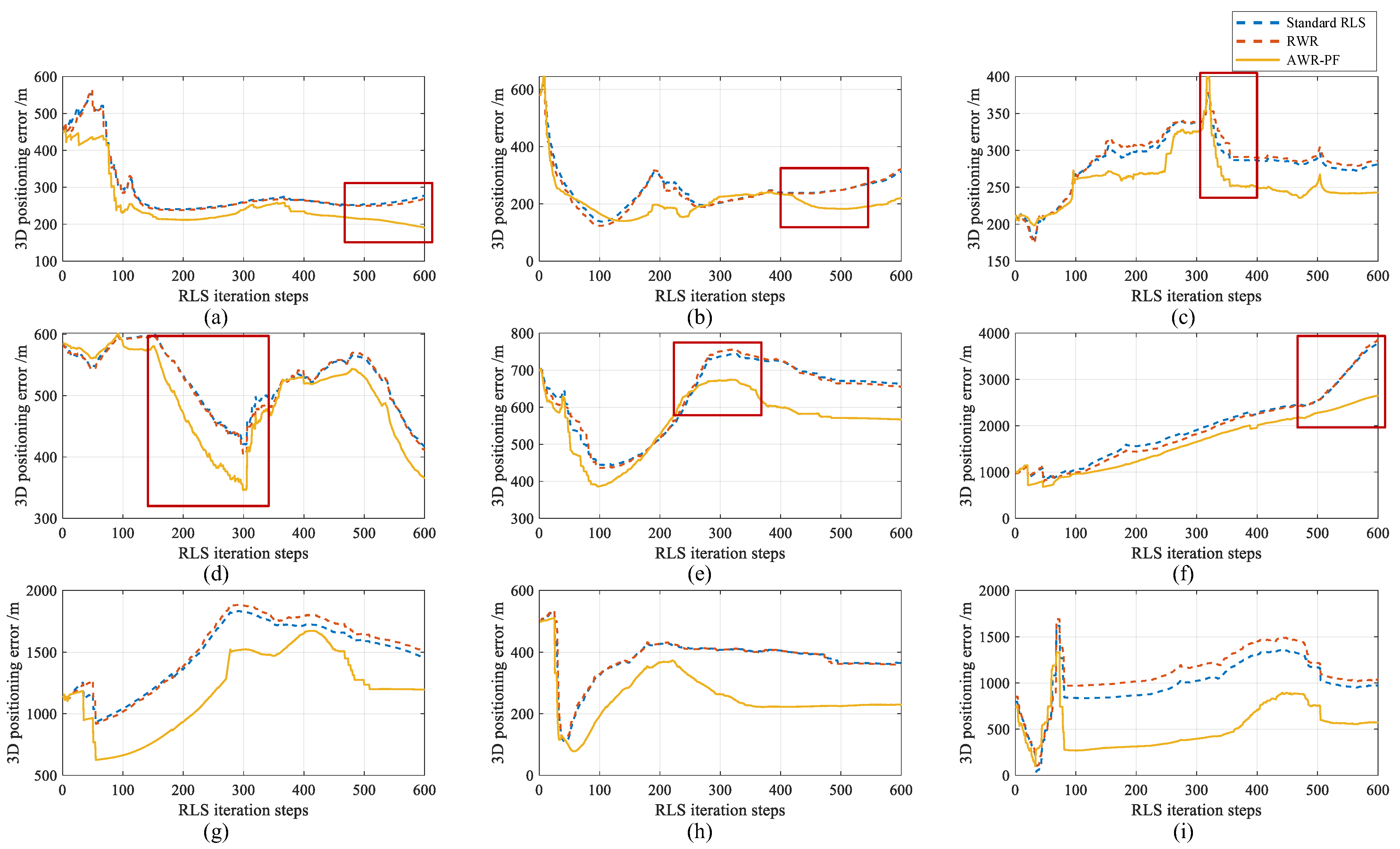
Experimental results from individual positioning trials demonstrate that the proposed AWR-PF achieved a maximum reduction of 45.15% in final error in single positioning trials compared to the standard RLS. As illustrated in Figure 16, representative positioning cases were selected to showcase the superior policy learned by the agent. The agent exhibited remarkable adaptability when processing complex epoch information, dynamically adjusting weighting parameters to optimize positioning accuracy across varying scenarios. The AWR-PF demonstrated adaptive weighting capability by dynamically reducing epoch weights when quality deteriorated (increasing positioning errors) to mitigate accuracy degradation (Figure 16e,f), while increasing weights for high-quality epochs (decreasing errors) to enhance their contribution to the positioning solution, thereby optimizing overall accuracy (Figure 16c,d). The AWR-PF’s weighting strategy demonstrated exceptional robustness by nearly completely mitigating the adverse effects of severely degraded epochs (Figure 16a,b). Consequently, while both standard RLS and RWR exhibited increasing positioning errors under such conditions, the proposed AWR-PF maintained continuous error reduction. Moreover, in additional positioning experiments, the AWR-PF fully leveraged its temporal dependency-aware decision-making capability to dynamically modulate weighting strategies, resulting in comprehensively superior positioning accuracy throughout the entire RLS iterative process compared to both standard RLS and RWR approaches (Figure 16g–i).
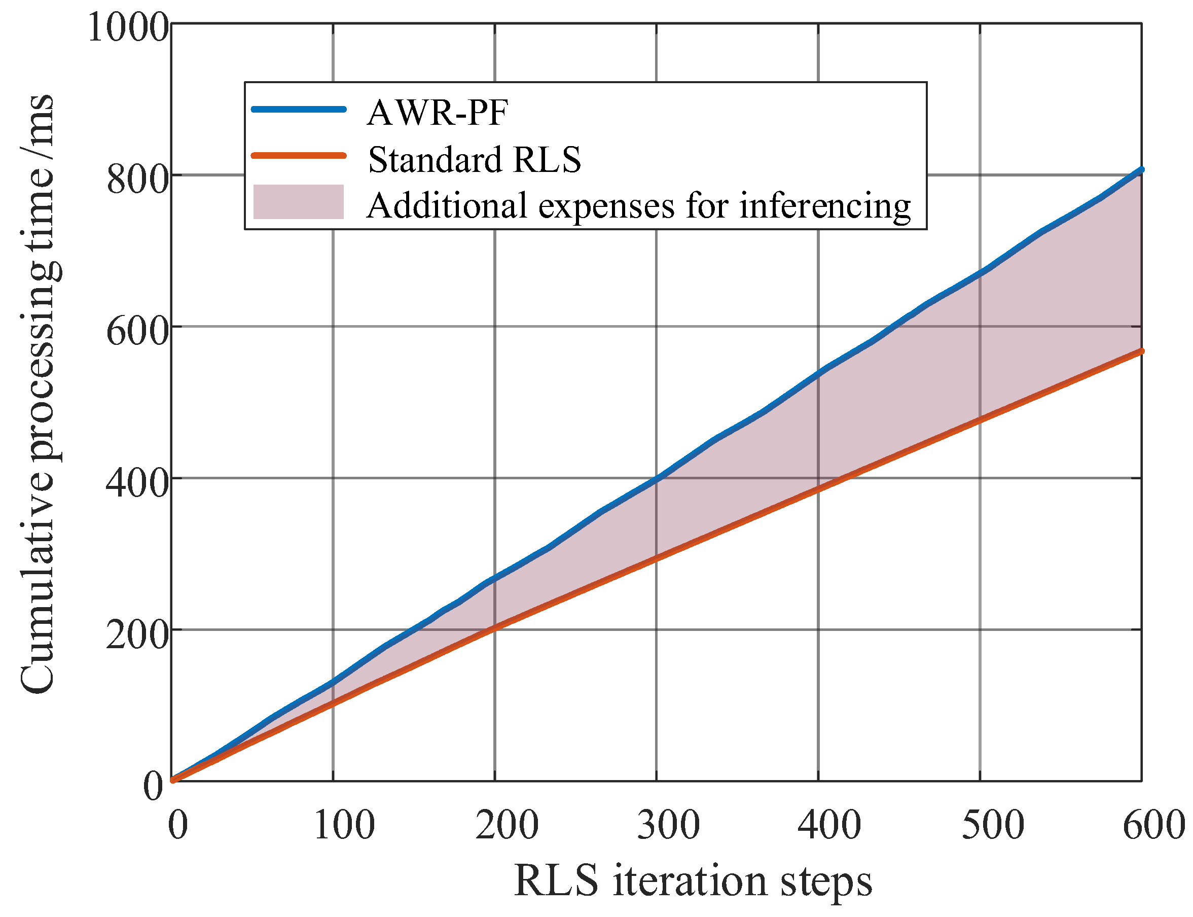
Furthermore, we analyzed the agent’s inference latency and computational overhead to demonstrate AWR-PF’s practical feasibility. First, we recorded average processing times for the AWR-PF and standard RLS during the testing phase (Figure 17). Results indicate that under current desktop computing configurations, the AWR-PF required approximately 0.4 ms for inference in each iteration step, while standard RLS consumed about 0.95 ms per iteration step. The agent’s inference latency constituted roughly 30% of total computation time, demonstrating efficient processing enabled by our lightweight network architecture. Second, we estimated computational overhead based on network design. Given our fully connected layers, each neuronal connection involved one multiplication and one addition operation. The total number of floating point operations for each inference was 2 × ( 9 × 256 + 256 × 256 + 256 × 20 ) = 145,920 . This represents negligible computational demand for modern processors. Collectively, these results confirm the technical viability of deploying our intelligent agent in practical engineering applications.

6. Discussion

6.1. A Comparative Discussion with the Results of Other Methods

At present, in the field of LEO SOP positioning, the research on epoch weighting and screening is relatively scarce, mainly focusing on satellite screening based on geometric configuration and weighting based on orbital error. It is not difficult to find that the existing LEO SOP weighting methods all have essential differences from the method proposed in this paper, which are specifically reflected in the following two points:
  • Current research can only screen satellites, while this paper delves into the weighting of each epoch of satellites.
  • The current research only optimizes based on one or two aspects of parameters, while this paper comprehensively considers nine parameters at four levels.
Furthermore, the use of different constellations and the opacity of engineering details makes it extremely difficult to reproduce algorithms in the same field under strictly con-trolled variables. Based on the above discussion, it is difficult for this paper to make an effective comparison with existing algorithms.
In this work, the test set covers almost all time periods of the 24 h of the day, with an observation duration of 27 h and a total of 80,764 epochs. Among the 97 independent LEO SOP locations examined during the observation period, the AWR-PF outperformed RLR and standard RLS on average. This indicates that the improvement in positioning accuracy by the AWR-PF is not an accidental phenomenon but a fact verified through a large number of experiments.
All the positioning comparisons in the paper have undergone strict variable control. That is, the only difference among the three methods lies in the weighting strategies for epoch elements (weighted by the agent, randomly weighted, and with a constant weight of 1). The results obtained from this comparison demonstrate that the weighting strategy of the agent optimizes the positioning results rather than due to other factors. This also supports the core innovation point of this article: an agent capable of weighting the fusion of multiple characteristics of epoch elements.

6.2. Future Work

Future research may explore migrating the agent from LEO SOP to MEO or GEO SOP scenarios, necessitating adaptation to altered observation characteristics. In MEO and GEO environments, geometric configuration changes will substantially reduce Doppler frequency fluctuations while moderating SNR variations. Consequently, the agent must undergo retraining using MEO/GEO-specific signals. Through this process, the agent will recalibrate its network parameters by enhancing Doppler frequency sensitivity while desensitizing to SNR changes, thereby maintaining effective collaboration with RLS within the AWR-PF. This adaptive retraining ensures optimal performance across distinct orbital regimes despite fundamental differences in signal dynamics.
The reward function in this study relies on positioning error, which poses implementation challenges in GNSS-denied environments, where true position is typically unavailable. This limitation necessitates developing truth-position-independent reward mechanisms for practical deployment. Notably, GDOP offers a significant advantage: Calculated solely from satellite geometry without requiring true position, it quantifies positioning solution sensitivity to measurement errors. This characteristic establishes GDOP as an effective indirect quality metric for epoch assessment. Empirical evidence further indicates that SNR and elevation angle critically influence epoch quality, with both being directly measurable from non-cooperative SOP. Consequently, future research should focus on designing reward mechanisms based on GDOP, SNR, and elevation angle—for instance, assigning higher rewards to epochs exhibiting lower GDOP, higher SNR, and larger elevation angles.
To enhance the agent’s versatility, future work could involve multi-constellation training across diverse locations and receivers. Our trained agent currently supports real-time positioning using Iridium signals with RLS at any time near the training location via corresponding receivers. However, significant changes in location (beyond 500 km), receiver hardware, or satellite constellations (e.g., switching to Starlink or OneWeb) necessitate agent retraining. Three primary factors challenge generalization: Location shifts (>500 km) alter ionospheric/tropospheric conditions, receiver variations introduce antenna gain/phase response discrepancies, and constellation differences fundamentally change geometric configurations. Achieving universal positioning—any location, any receiver, any constellation—requires more extensive and diverse training data. This expansion would simultaneously pose greater demands on MDP design and DRL algorithm performance to maintain robustness across such heterogeneous operational environments. Future implementations must address these scalability challenges to realize truly adaptable navigation agents.
7. Conclusions

This study systematically identifies nine-dimensional characteristic space characterizing Iridium epochs through extensive empirical measurements and positioning experiments with Iridium signals. Building upon this foundation, an innovative Agent-Weighted RLS Positioning Framework (AWR-PF) is proposed, where an agent dynamically adjusts epoch-specific weights in real time based on characteristic variations to enhance positioning accuracy through RLS iterations. Statistical results from 97 independent experiments demonstrate that the AWR-PF achieves superior positioning accuracy compared to standard RLS. Detailed case-by-case analysis further reveals the trained agent’s capability to adaptively modulate weights according to variations within the 9D characteristic space, exhibiting remarkable algorithmic robustness. This work represents the first successful integration of AI algorithms as the core decision-maker in LEO SOP positioning, demonstrating promising initial results. Future refinements in modeling, AI training algorithm selection, and hyperparameter optimization will further unlock the potential of the proposed framework.

Author Contributions

Writing—original draft preparation, methodology, and validation, J.Y.; writing—original draft preparation, methodology, and validation, F.L.; conceptualization, original idea, supervision, writing—review, R.L.; writing—review and editing X.C.; investigation, L.Z.; supervision, H.Y.; project administration, G.Y. All authors have read and agreed to the published version of the manuscript.

Funding

This research was supported by the Specialized Research Fund for State Key Laboratory of Solar Activity and Space Weather.

Data Availability Statement

The raw data supporting the conclusions of this article will be made available by the authors on request.

Acknowledgments

This research has no additional acknowledgments for institutions or individuals.

Conflicts of Interest

The authors declare no conflicts of interest.

References

  1. Langley, R.B.; Teunissen, P.J.G.; Montenbruck, O. Introduction to GNSS. In Springer Handbook of Global Navigation Satellite Systems; Springer: Cham, Switherland, 2017; pp. 3–23. [Google Scholar]
  2. Yun, J.; Lim, C.; Park, B. Inherent limitations of Smartphone GNSS Positioning and effective methods to increase the accuracy utilizing dual-frequency measurements. Sensors 2022, 22, 9879. [Google Scholar] [CrossRef]
  3. Kaplan, E.D.; Hegarty, C.J. Understanding GPS: Principles and Applications, 2nd ed; Artech House: Norwood, MA, USA, 2006; pp. 14–16. [Google Scholar]
  4. Grenier, A.; Lohan, E.S.; Ometov, A.; Nurmi, J. A Survey on Low-Power GNSS. IEEE Commun. Surv. Tutor. 2023, 25, 1482–1509. [Google Scholar] [CrossRef]
  5. Puricer, P.; Kovar, P. Technical limitations of GNSS receivers in indoor positioning. In Proceedings of the 2007 17th International Conference Radioelektronika, Brno, Czech Republic, 24–25 April 2007. [Google Scholar]
  6. Hall, T.D. Radiolocation Using AM Broadcast Signals. Ph.D. Thesis, Massachusetts Institute of Technology, Cambridge, MA, USA, 2002. [Google Scholar]
  7. He, S.; Chan, S.H.G. Wi-Fi fingerprint-based indoor positioning: Recent advances and comparisons. IEEE Commun. Surv. Tutor. 2015, 18, 466–490. [Google Scholar] [CrossRef]
  8. Kraus, T.; Bochkati, M.; Maia, C.A.S.; Lapadat, A.; Cimbaljevic, M.; Mitic, A.; Dütsch, N.; Pany, T. Development of a Front end with GNSS, 4G/5G, any Other SOOP and IMU Support by a Customized SDR. In Proceedings of the 2024 International Technical Meeting of The Institute of Navigation, Long Beach, CA, USA, 23–25 January 2024. [Google Scholar]
  9. Carter, K.L.; Ramlall, R.; Tummala, M.; McEachen, J. Bandwidth efficient ATSC TDOA positioning in GPS-denied environments. In Proceedings of the 2013 International Technical Meeting of The Institute of Navigation, San Diego, CA, USA, 28–30 January 2013. [Google Scholar]
  10. Du, Y.; Qin, H.; Li, J.; Xu, Z.; Su, Y. LEOS-SOP/INS Integrated Differential Positioning Based on Non-parallel Line-of-sight Vectors and Orbit errors Correction. IEEE Sens. J. 2024, 25, 1266–1278. [Google Scholar] [CrossRef]
  11. Xie, H.; Zhan, Y.; Zeng, G.; Pan, X. LEO mega-constellations for 6G global coverage: Challenges and opportunities. IEEE Access 2021, 9, 164223–164244. [Google Scholar] [CrossRef]
  12. Okati, N.; Riihonen, T. Nonhomogeneous stochastic geometry analysis of massive LEO communication constellations. IEEE Trans. Commun. 2022, 70, 1848–1860. [Google Scholar] [CrossRef]
  13. Goh, S.T.; Zekavat, S.A.; Abdelkhalik, O. LEO satellite formation for SSP: Energy and doppler analysis. IEEE Trans. Aerosp. Electron. Syst. 2015, 51, 18–30. [Google Scholar] [CrossRef]
  14. Gao, L.; Tong, F.; Li, J.; Chen, L. Analysis and simulation of Doppler shift of LEO satellite. In International Conference on Wireless Communications, Networking and Applications; Springer Nature: Singapore, 2022. [Google Scholar]
  15. Neinavaie, M.; Shadram, Z.; Kozhaya, S.; Kassas, Z.M. First results of differential Doppler positioning with unknown Starlink satellite signals. In Proceedings of the 2022 IEEE Aerospace Conference (AERO), Big Sky, MT, USA, 5–12 March 2022. [Google Scholar]
  16. Farhangian, F.; Landry, R., Jr. Multi-constellation software-defined receiver for Doppler positioning with LEO satellites. Sensors 2020, 20, 5866. [Google Scholar] [CrossRef]
  17. Jardak, N.; Adam, R.; Jault, Q. Leveraging Multi-LEO Satellite Signals for Opportunistic Positioning. IEEE Access 2024, 12, 127100–127114. [Google Scholar] [CrossRef]
  18. Wang, X.; Zhao, Y.; Lin, G.; Zhou, J. Navigation and positioning with multi-constellation LEO satellite collaboration signals. In Proceedings of the China Conference on Command and Control; Springer Nature: Singapore, 2024. [Google Scholar]
  19. Haidar-Ahmad, J.; Khairallah, N.; Kassas, Z.M. A hybrid analytical-machine learning approach for LEO satellite orbit prediction. In Proceedings of the 2022 25th International Conference on Information Fusion (FUSION), Linköping, Sweden, 4–7 July 2022. [Google Scholar]
  20. Fan, G.; Chen, X.; Chen, Z.; Zhang, R.; Wu, P.; Wei, Q.; Xu, W.; Dai, J. Toward Massive Satellite Signals of Opportunity Positioning: Challenges, Methods, and Experiments. Space Sci. Technol. 2024, 4, 0191. [Google Scholar] [CrossRef]
  21. Wang, D.; Qin, H.; Huang, Z. Doppler positioning of LEO satellites based on orbit error compensation and weighting. IEEE Trans. Instrum. Meas. 2023, 72, 5502911. [Google Scholar] [CrossRef]
  22. Kassas, Z.M.; Hayek, S.; Ahmad, J.H. LEO satellite orbit prediction via closed-loop machine learning with application to opportunistic navigation. IEEE Aerosp. Electron. Syst. Mag. 2024, 40, 34–49. [Google Scholar] [CrossRef]
  23. Zhao, C.; Qin, H.; Wu, N.; Wang, D. Analysis of baseline impact on differential doppler positioning and performance improvement method for LEO opportunistic navigation. IEEE Trans. Instrum. Meas. 2023, 72, 8501110. [Google Scholar] [CrossRef]
  24. Allahvirdi-Zadeh, A.; El-Mowafy, A.; Wang, K. Doppler Positioning Using Multi-Constellation LEO Satellite Broadband Signals as Signals of Opportunity. Navig. J. Inst. Navig. 2025, 72, navi.691. [Google Scholar] [CrossRef]
  25. Saroufim, J.; Hayek, S.; Kassas, Z. Analysis of satellite ephemeris error in differential and non-differential navigation with LEO satellites. In Proceedings of the IEEE Aerospace Conference, Big Sky, MT, USA, 2–9 March 2024. [Google Scholar]
  26. Wei, Q.; Chen, X.; Zhan, Y.F. Exploring implicit pilots for precise estimation of LEO satellite downlink Doppler frequency. IEEE Commun. Lett. 2020, 24, 2270–2274. [Google Scholar] [CrossRef]
  27. Tan, Z.; Qin, H.; Cong, L.; Zhao, C. Positioning using IRIDIUM satellite signals of opportunity in weak signal environment. Electronics 2019, 9, 37. [Google Scholar] [CrossRef]
  28. Huang, C.; Qin, H.; Zhao, C.; Liang, H. Phase-time method: Accurate Doppler measurement for Iridium NEXT signals. IEEE Trans. Aerosp. Electron. Syst. 2022, 58, 5954–5962. [Google Scholar] [CrossRef]
  29. Mnih, V.; Kavukcuoglu, K.; Silver, D.; Graves, A.; Antonoglou, I.; Wierstra, D.; Riedmiller, M. Playing atari with deep reinforcement learning. arXiv 2013, arXiv:1312.5602. [Google Scholar] [CrossRef]
  30. Van Hasselt, H.; Guez, A.; Silver, D. Deep reinforcement learning with double q-learning. In Proceedings of the AAAI Conference on Artificial Intelligence, Phoenix, AZ, USA, 12–17 February 2016; Volume 30. [Google Scholar]
  31. Zhao, C.; Qin, H.; Li, Z. Doppler measurements from multiconstellations in opportunistic navigation. IEEE Trans. Instrum. Meas. 2022, 71, 8500709. [Google Scholar] [CrossRef]
  32. Yang, M.; Wang, Y.; Fang, Z.; Chen, J.; Liu, Y.; Lei, M.; Xu, Y. A Novel Doppler Estimation Approach Using ORBCOMM Signals for High-Precision Positioning. Electronics 2024, 13, 4882. [Google Scholar] [CrossRef]
  33. McLemore, B.; Psiaki, M.L. GDOP of Navigation using Pseudorange and Doppler Shift from a LEO Constellation. In Proceedings of the 34th International Technical Meeting of the Satellite Division of The Institute of Navigation (ION GNSS+ 2021), St. Louis, MO, USA, 20–24 September 2021. [Google Scholar]
  34. Psiaki, M.L. Navigation using carrier Doppler shift from a LEO constellation: TRANSIT on steroids. Navigation 2021, 68, 621–641. [Google Scholar] [CrossRef]
Figure 1. The orbital errors predicted using the Simplified General Perturbations Version 4 (SGP4) model. (a) Three-dimensional position errors; (b) three-dimensional velocity errors.
Remotesensing 17 02692 g001
Figure 2. The variation curves of geometric dilution of precision (GDOP) and positioning errors versus epoch similarity derived from 500 real-world Iridium signal positioning trials.
Remotesensing 17 02692 g002
Figure 3. The signal-to-noise ratio (SNR) of each real Iridium epoch during the 2 min observation window.
Remotesensing 17 02692 g003
Figure 4. The simulation results of temporal evolution of both Doppler frequency and Doppler rate. (a) Doppler frequency and Doppler rate as functions of time; (b) the simulated sky map of temporal evolution.
Remotesensing 17 02692 g004
Figure 5. The diagram of the proposed Agent-Weighted RLS Positioning Framework.
Remotesensing 17 02692 g005
Figure 6. The diagram of the dynamic Bayesian network (DBN) corresponding to the proposed MDP model. Solid arrows indicate direct operations, while dashed arrows indicate indirect influences.
Remotesensing 17 02692 g006
Figure 7. Single training process of Double Deep Q-Network-based Epoch Weighting (DDQN-EW) algorithm. Boxes of the same color indicate the same structure.
Remotesensing 17 02692 g007
Figure 8. The Iridium signal reception and processing platform. (a) Platform deployment scenario; (b) platform configuration.
Remotesensing 17 02692 g008
Figure 9. The distribution of signal reception windows of the training set and the test set.
Remotesensing 17 02692 g009
Figure 10. The characteristic statistics of the captured Iridium epsochs. (a) SNR; (b) Doppler frequency; (c) ephemeris age; (d) azimuth angle; (e) elevation angle; (f) satellite-to-receiver distance; (g) satellite ID.
Remotesensing 17 02692 g010
Figure 11. Agent’s per-timestep average cumulative reward during training. The dotted line indicates that the average cumulative rewards obtained by the agent after this step tend to stabilize.
Remotesensing 17 02692 g011
Figure 12. Comparison of positioning performance with different weighting strategies during training.
Remotesensing 17 02692 g012
Figure 13. Agent’s per-timestep average cumulative reward during testing. The dotted line indicates that the average cumulative rewards obtained by the agent after this step tend to stabilize.
Remotesensing 17 02692 g013
Figure 14. Comparison of positioning performance with different positioning methods during testing: standard RLS, randomly weighted RLS (RWR), and proposed AWR-PF.
Remotesensing 17 02692 g014
Figure 15. Performance comparison of three positioning methods during testing from the standard RLS’s perspective.
Remotesensing 17 02692 g015
Figure 16. Comparative analysis of typical single positioning trial errors reveals distinct performance patterns. The red box indicates that during these periods, the agent’s decision-making demonstrated particular advantages. (a,b) While positioning errors increase with the standard RLS, they demonstrate consistent reduction with the AWR-PF; (c,d) the AWR-PF approach achieves faster error reduction compared to the standard RLS; (e,f) the AWR-PF approach achieves slower error improvement compared to the standard RLS; (gi) the AWR-PF maintains superior positioning accuracy throughout the entire iteration.
Remotesensing 17 02692 g016
Figure 17. Comparison of average processing time with standard RLS and proposed AWR-PF during testing.
Remotesensing 17 02692 g017
Table 1. The Markov Decision Process (MDP) elements of using Deep Reinforcement Learning (DRL) to train agents to optimize low Earth orbit (LEO) signal of opportunity (SOP) positioning using Recursive Least Squares (RLS).
MDP ElementsLEO SOP Positioning Task
EnvironmentAgent-weighted RLS Positioning Framework
AgentTrained neural network
StatesEpoch characteristics and geometry dilution of precision
ActionsEpoch weighting decisions
RewardsVariation in positioning error
PolicyEpoch weighting policy
Table 2. Environment parameters and hyper-parameters for training.
ParameterValueDescription
M 1 200The number of epochs used for initial positioning.
M 2 600The number of epochs used for agent decision-making.
H 1 256The number of neurons in the first hidden layer.
H 2 256The number of neurons in the second hidden layer.
k 1 5Reward coefficient associated with the absolute change in positioning error.
k 2 1000Reward coefficient associated with the percentage change in positioning error.
σ 0.01Minimum offset term.
γ 0.8Discount factor, which quantifies the importance of future rewards.
N D 10,000Experience replay buffer capacity.
N B 64Number of samples per mini-batch.
τ 0.01Target network update coefficient.
ε min 0.01Minimum exploration rate.
λ 0.99995The decay rate of the exploration rate.
α 0.0005The learning rate of the Adam optimizer.
Disclaimer/Publisher’s Note: The statements, opinions and data contained in all publications are solely those of the individual author(s) and contributor(s) and not of MDPI and/or the editor(s). MDPI and/or the editor(s) disclaim responsibility for any injury to people or property resulting from any ideas, methods, instructions or products referred to in the content.