Abstract
Accurate and timely estimation of soybean emergence at the plot scale using unmanned aerial vehicle (UAV) remote sensing imagery is essential for germplasm evaluation in breeding programs, where breeders prioritize overall plot-scale emergence rates over subimage-based counts. This study proposes PlotCounter, a deep learning regression model based on the TasselNetV2++ architecture, designed for plot-scale soybean seedling counting. It employs a patch-based training strategy combined with full-plot validation to achieve reliable performance with limited breeding plot data. To incorporate additional agronomic information, PlotCounter is extended into a multitask learning framework (MTL-PlotCounter) that integrates sowing metadata such as variety, number of seeds per hole, and sowing density as auxiliary classification tasks. RGB images of 54 breeding plots were captured in 2023 using a DJI Mavic 2 Pro UAV and processed into an orthomosaic for model development and evaluation, showing effective performance. PlotCounter achieves a root mean square error (RMSE) of 6.98 and a relative RMSE (rRMSE) of 6.93%. The variety-integrated MTL-PlotCounter, V-MTL-PlotCounter, performs the best, with relative reductions of 8.74% in RMSE and 3.03% in rRMSE compared to PlotCounter, and outperforms representative YOLO-based models. Additionally, both PlotCounter and V-MTL-PlotCounter are deployed on a web-based platform, enabling users to upload images via an interactive interface, automatically count seedlings, and analyze plot-scale emergence, powered by a multimodal large language model. This study highlights the potential of integrating UAV remote sensing, agronomic metadata, specialized deep learning models, and multimodal large language models for advanced crop monitoring.
1. Introduction
Soybean (Glycine max [L.] Merr.), a major global oilseed crop and protein source, is crucial for agricultural sustainability and food security [1,2]. In soybean breeding work, precise seedling counting is a key step, as it forms the basis for evaluating germplasm quality and is an important criterion for selecting superior varieties [3]. Traditionally, seedling counting is conducted by sampling selected field locations and estimating the total number from these observations, a process that is both labor-intensive and prone to error in complex field environments. Therefore, developing an efficient and accurate automated seedling counting method is crucial. Furthermore, creating an automated seedling counting platform tailored for agricultural breeding settings offers an ideal solution.
In addition to manual counting, various classical image processing techniques have been applied to seedling counting. Liu et al. [4] extracted wheat seedlings from RGB images captured by a digital camera and counted them using excess green and Otsu’s thresholding methods, followed by skeleton optimization. Gnädinger and Schmidhalter [5] performed automated maize plant counting using RGB imagery captured by an unmanned aerial vehicle (UAV), applying decorrelation stretch, HSV thresholding, and pixel clustering. Koh et al. [6] estimated safflower seedling density through object-based image analysis combined with template matching applied to UAV RGB images. Furthermore, Liu et al. [7] demonstrated that traditional methods such as corner detection and linear regression can also achieve high accuracy in maize seedling counting using UAV imagery.
In recent years, UAV remote sensing [8] platforms equipped with cameras have facilitated the rapid and high-throughput acquisition of images from large-scale agricultural fields, providing robust technical support for crop seedling monitoring [9]. In such applications, orthomosaic maps have become widely used as fundamental data products. The generation of orthomosaics typically follows a standard workflow that begins with flight planning and UAV image acquisition over the target area, followed by photogrammetric processing, which includes image alignment and mosaicking [10]. These orthomosaics allow agricultural researchers and plant breeders to analyze phenotypic data efficiently and nondestructively [11]. Depending on the sensors mounted on UAVs, remote sensing images may include RGB [12], multispectral [13], or hyperspectral data [14], offering diverse options for crop monitoring and seedling assessment.
In crop seedling counting based on UAV remote sensing, deep learning techniques have played a crucial role [15,16], with RGB imagery serving as the most cost-effective data source [17,18]. Oh et al. [19] developed a method for separating, locating, and counting cotton seedlings using an improved YOLOv3 [20]. Barreto et al. [21] proposed a sugar beet seedling counting model based on a fully convolutional network (FCN) and demonstrated that extending the previously trained FCN pipeline to other crops was possible with a small training dataset. Chen et al. [22] introduced a cabbage seedling counting method by modifying YOLOv8n [23], where a Swin-conv block replaced the C2f block in the backbone, and ParNet attention modules were incorporated into both the backbone and neck parts, enabling accurate tracking and counting of cabbage seedlings. Shahid et al. [24] utilized U-Net [25] and YOLOv7 [26] as plant detection modules for tobacco counting and found the real-time system using YOLOv7 and SORT to be the most effective. Building on TasselNetV2+ [27], Xue et al. [28] proposed the TasselNetV2++ model, which demonstrated strong counting performance for soybean seedlings, maize tassels, sorghum heads, and wheat heads. De Souza et al. [29] employed a multilayer perceptron to classify and count soybean seedlings using RGB and multispectral images with seedlings ranging from 10 to 25.
Among crop seedling counting methods based on UAV and deep learning, detection-based counting methods using the YOLO series have been most widely applied. These methods can simultaneously locate and count seedlings. However, the counting process relies on detection results and is not an end-to-end counting approach. In agricultural scenarios with severe occlusions, segmentation-based models encounter difficulties with sample annotation and target separation. Regression-based crop counting models can directly regress counting results from input images, representing an end-to-end counting method. Among them, TasselNetV2++ exhibited strong adaptability to multiple crops and varying input sizes. However, TasselNetV2++ also achieved counting for small images containing 0 to 22 soybean seedlings. In breeding practices, it is the seedling count and emergence rate per plot that truly matter, not the number of seedlings in each small image.
Although the aforementioned deep learning-based crop counting methods have achieved good performance, they can still be further optimized by incorporating additional information. Multitask learning (MTL) is a method for integrating multi-source information into deep learning models. It can improve model generalization and accuracy by sharing information across related tasks, compared to learning each task independently [30,31]. In the field of crop counting, multitask learning has proven to be an effective approach for integrating information. Pound et al. [32] employed MTL for wheat head counting and classification of images with or without awns, showcasing the potential of MTL in plant phenotyping. Dobrescu et al. [33] used MTL to simultaneously extract different phenotypic traits from plant images and predict three traits: leaf count, leaf area, and genotype category. It demonstrated that jointly learning multiple related tasks can reduce leaf counting errors. Jiao et al. [34] introduced confidence scores as a classification head based on YOLOX [35], improving counting performance by removing redundant detection boxes with classification confidence scores lower than 0.3 during the wheat head counting process. These MTL models generally require both input images and multitask ground truth during training. However, in practical use, only images are needed as input for the trained model to perform the counting task, eliminating the need for additional multitask information.
To provide an intuitive user interface and automated analysis capability, researchers have also focused on model deployment and application. Li and Yang [36] developed a few-shot cotton pest recognition model and integrated an intelligent recognition system into embedded hardware for practical agricultural applications. Sun et al. [37] developed a PC-based software application to extract phenotypic traits from images of rice panicles captured by smartphones, facilitating the analysis of panicle characteristics. To achieve high-precision simultaneous detection of mango fruits and fruiting stems on an edge computing platform, Gu et al. [38] improved the YOLOv8n model and deployed it on both PC and NVIDIA Jetson Orin Nano platforms. Xu et al. [39] developed a real-time pest detection algorithm based on YOLOv5s [40] with the lightweight GhostNet network, optimized its neck and head structures, and deployed the model as an Android application.
The development of large language models (LLMs) and other generative artificial intelligence (AI) has opened new opportunities [41]. Zhu et al. [42] proposed a multimodal model for potato disease detection, integrating a visual branch, a text description branch, and an image statistical feature branch. Based on this model and GPT-4, they developed an expert system for potato disease diagnosis and control. This system can utilize the LLM to offer suggestions for potato disease control, enabling real-time interaction with control recommendations. The LLM can serve as a useful explainer for the output of the self-built model. Moreover, deploying the self-built model with LLM embedding can enhance consultations by providing all necessary information, facilitating real-world applications.
Therefore, the objectives of this study are as follows: (1) achieve end-to-end soybean seedling counting at the plot scale based on TasselNetV2++, named PlotCounter; (2) explore the incorporation of sowing-related information into PlotCounter during the training stage via multitask learning, through category information integration, classifier design, and loss function construction, referred to as MTL-PlotCounter; and (3) develop web-based plot-scale seedling counting agents based on a multimodal LLM and evaluate their performance using a UAV-derived dataset tailored for plot-scale soybean seedling counting.
2. Materials and Methods
2.1. Dataset Preparation
2.1.1. Study Area and Experimental Design
The experiments were carried out in a soybean breeding field in Jinzhong, Shanxi Province, China (37°26′0.9″N–37°26′2.5″N, 112°35′39.9″E–112°35′40.4″E), located within a temperate continental climate zone that experiences an average annual temperature of 10.4 °C and 462 mm of precipitation.
In 2023, a randomized experiment with replications was conducted to evaluate the emergence performance of soybean under different varieties, numbers of seeds per hole (NSPH), and sowing densities. The soybean varieties selected for the experiment were “Dongdou 1” and “Tiefeng 31”, which are the primary varieties promoted in Jinzhong. The experiment simulated precision sowing with 1, 2, and 3 seeds per hole and tested three sowing densities: 120,000, 154,000, and 222,000 seeds per hectare (ha−1). Table 1 presented the hole spacing derived from NSPH values corresponding to various sowing densities with a fixed row spacing of 50 cm. The field experiment tested two soybean varieties under a factorial design combining three NSPH levels and three sowing densities. Each treatment was replicated three times, yielding a total of 54 breeding plots.

Table 1.
Hole spacing derived from numbers of seeds per hole corresponding to various sowing densities.
2.1.2. Plot-Scale Soybean Seedling Dataset Construction
A DJI Mavic 2 Pro UAV (SZ DJI Technology Co., Shenzhen, China) equipped with a Hasselblad L1D-20C camera (SZ DJI Technology Co., Shenzhen, China) was used to capture RGB imagery. Flights were conducted at 5 m altitude with a speed of 2 m/s, achieving a ground sampling distance of 0.1 cm/pixel. Imaging was performed with the camera oriented downward before sunrise (22 June 2023, 5:30–6:00 AM, 16 days after sowing) to minimize shadows, with front and side overlap rates of 75% and 60%, respectively. Based on preliminary tests, a flight height of 5 m was selected to ensure sufficient image resolution and meet the UAV minimum requirement for image stitching. The images were stitched into a TIF format mosaic image using the DJI Smart Agriculture Platform (SZ DJI Technology Co., Ltd., Shenzhen, China).
Individual plot images were extracted from the stitched mosaic image and resized to 3072 × 6144 pixels via zero-padding to standardize their dimensions. The seedling counts per plot ranged from 55 to 211, with a total of 5932 seedlings annotated across all images. Due to significant mutual occlusion among seedlings in the UAV imagery captured after no new soybean seedling emerged, direct image annotation was infeasible, necessitating field-based labeling. Each soybean seedling was manually annotated in the field using printed high-resolution plot images, and the bounding boxes were later converted into dot annotations indicating seedling centroids. Figure 1 showed the field data acquisition and experimental site overview.
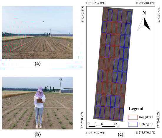
Figure 1.
Field data acquisition and experimental site overview. (a) UAV image acquisition. (b) Field investigation. (c) Experimental site location and plot layout.
Additionally, sowing-related information, including the soybean variety, NSPH, and sowing density for each plot, was recorded in the form of a dictionary, where the key was the plot ID and the values were sets containing the labels for the soybean variety, NSPH, and sowing density. The plot-scale soybean seedling dataset consists of images of 54 plots, dot annotation data for each seedling, as well as soybean variety, NSPH, and sowing density information for each plot. All 54 plots were used in the study and were divided into training, validation, and testing sets for model development and evaluation.
Given that NSPH significantly affected the occlusion level among seedlings, the dataset was partitioned by NSPH to ensure model generalizability. Specifically, from each NSPH category, 10 plots were assigned to the training set, 4 plots to the validation set, and 4 plots to the testing set. Consequently, for the three NSPH levels, the training set comprised 30 plots, while the validation and testing sets each contained 12 plots.
2.2. TasselNetV2++
TasselNetV2++ was composed of three concatenated components: an encoder, a counter, and a normalizer, with its network architecture illustrated in Figure 2. Initially, the encoder adopted a dual-branch architecture. One branch comprised three Conv-CBAM-Pool blocks and two Conv-CBAM blocks, while the other branch employed a simplified version of the YOLOv5s backbone tailored for this architecture. The encoder extracted features through gathering and distribution (GD), fusion via bilinear interpolation, average pooling (AvgPool), and feature concatenation, followed by a low-stage information fusion module (Low-IFM) [43]. In the counter component, the features were transformed into a redundant count map using AvgPool, a Conv-BN-SiLU (CBS) block, a convolutional block attention module (CBAM) [44], a Conv-BN-ReLU (CBR) block, and a final convolutional layer. A normalizer then converted this into the final count map, whose pixel sums yield each image’s seedling total. TasselNetV2++ proved robust across diverse tasks, including images with up to 22 soybean seedlings, but it has not yet been validated at the plot scale.
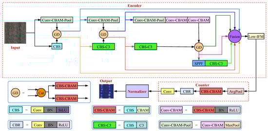
Figure 2.
The architecture of TasselNetV2++.
2.3. Plot-Scale Counting
2.3.1. Subimage Count Accumulation
Xue et al. [28] uniformly divided each plot image into 18 subimages and applied the TasselNetV2++ model to count the seedlings within these subimages. The most straightforward method for deriving plot-scale counting result from subimages is to directly accumulate the counting results of all subimages within a particular plot. The flowchart of the subimage count accumulation method was shown in Figure 3. As illustrated in Figure 3, each subimage of a plot was individually input into the TasselNetV2++ model to obtain its corresponding count. Subsequently, these individual counts were summed up to determine the total seedling count for the entire plot. Although the subimage count accumulation method is easy to operate, allowing for quick acquisition of counting results at the plot scale, it has some obvious limitations. One major issue was the possibility of counting the same soybean seedling twice in neighboring subimages. Moreover, during model validation, the global information at the plot scale was overlooked.
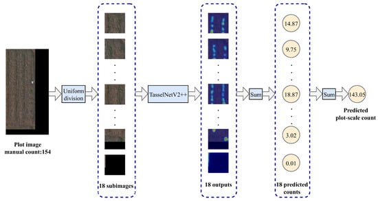
Figure 3.
The flowchart of the subimage count accumulation method.
2.3.2. PlotCounter
Although the subimage count accumulation method was a straightforward way to obtain counting results at the plot scale, the accumulation process inherently resulted in the accumulation of errors. As a result, outstanding subimage counting outcomes did not necessarily ensure superior counting results at the plot scale. PlotCounter aimed to achieve end-to-end seedling counting at the plot scale based on TasselNetV2++. Specifically, plot images were directly fed into the TasselNetV2++ model to obtain the counting results of soybean seedlings within the plot.
Currently, the training set comprises only 30 plots. Directly using these plot images for training would lead to an insufficient number of training samples, which would be inadequate for training a deep learning model. To address the issue of limited training plots, this study introduced a novel approach for organizing training samples. In each training epoch, 20 random patches per plot image were used as training samples. This method allowed for the generation of 600 randomly cropped image patches per training epoch. For model validation, the 12 plot images in the validation set were directly used to evaluate the model’s counting performance at the plot scale, helping to select the most suitable weights for the plot-scale counting task. The flowchart of PlotCounter was presented in Figure 4. As illustrated, PlotCounter employed this innovative sample organization strategy, where randomly cropped image patches from plot images were used for training, and the entire plot images were used for validation to obtain weights tailored for the plot-scale counting task. Consequently, by inputting the plot images from the test set into PlotCounter, the total number of seedlings in each plot can be obtained, achieving end-to-end plot-scale counting.
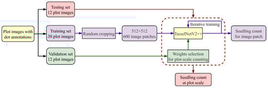
Figure 4.
The flowchart of PlotCounter.
2.4. MTL-PlotCounter
To enhance the accuracy of soybean seedling counting at the plot scale, this study explored the integration of sowing-related information during the training stage. During testing and practical applications, the model was expected to rely exclusively on plot images for counting, without requiring any additional sowing-related inputs. Multitask learning offered an efficient way to integrate various data sources, and during real-world applications, it eliminated the need to supply the model with agronomy data. Therefore, multitask learning was employed to incorporate sowing-related data.
Based on PlotCounter, the multitask driven plot-scale counting model was proposed, namely, MTL-PlotCounter. In MTL-PlotCounter, the main task was to count soybean seedlings at the plot scale, while the classification task served as an auxiliary task to improve counting accuracy. The overall framework of the proposed MTL-PlotCounter was illustrated in Figure 5. The encoder, counter, and normalizer components were consistent with those in TasselNetV2++ and PlotCounter. Similar to PlotCounter’s innovative sample organization strategy, MTL-PlotCounter randomly cropped image patches from plot images for training. Building upon PlotCounter, MTL-PlotCounter included a classifier that shared features extracted by the encoder with the counter.
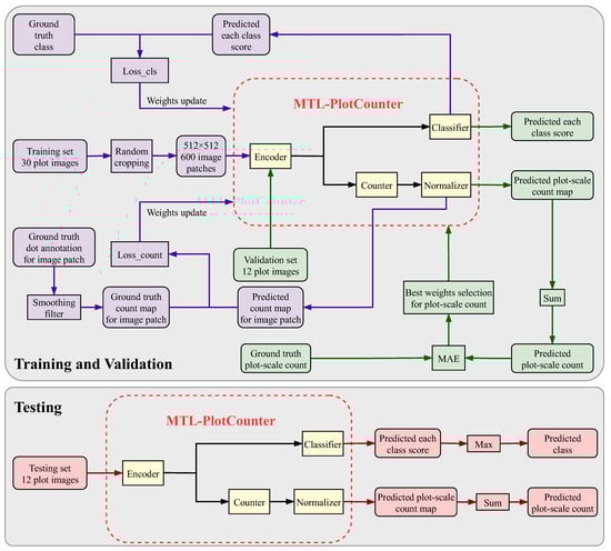
Figure 5.
Overall framework of the proposed MTL-PlotCounter.
As depicted in Figure 5, during the training process, the output for the counting task was the predicted count map for the image patch, while the output for the classification task was the predicted each class score. The counting loss was determined by the deviation between the predicted count map for the image patch and the corresponding ground truth count map, which was obtained through Gaussian smoothing and mean smoothing of the dot annotation image. The classification loss was determined by the deviation between the predicted class score and the ground truth class. Both the counting loss and the classification loss jointly updated the model weights, with the loss function optimizing both counting and classification tasks simultaneously.
As shown in Figure 5, during the validation process, directly inputting the plot image into MTL-PlotCounter can obtain the predicted count map and the class score for that plot. The predicted count for the plot was available by summing all the grayscale values in the predicted plot-scale count map. The best model weights for plot-scale counting were selected by calculating the mean absolute error (MAE) between the predicted counts and the ground truth counts for all plot samples in the validation set. The model weights were updated through training, and the most suitable weights for plot-scale counting were selected through validation. When tested, inputting the plot image into MTL-PlotCounter can predict the plot-scale count and plot category.
The field experimental design incorporated three factors, including soybean variety, NSPH, and sowing density. Utilizing these factors, we developed plot-scale soybean seedling counting models based on multitask learning, driven by variety, NSPH, and sowing density classifications. These models were named V-MTL-PlotCounter (variety driven MTL-PlotCounter), NSPH-MTL-PlotCounter (NSPH driven MTL-PlotCounter), and SD-MTL-PlotCounter (sowing density driven MTL-PlotCounter).
To develop the MTL-PlotCounter, three key issues needed to be solved. These involved integrating category information, designing an effective classifier, and formulating a loss function tailored for the multitask scenario. In the following, the implementation of V-MTL-PlotCounter, NSPH-MTL-PlotCounter, and SD-MTL-PlotCounter will be elaborated from these three aspects.
2.4.1. Category Information Incorporation
The plot IDs ranged from 1 to 54. The field experiment included two soybean varieties, labeled as 0 or 1, while both NSPH and sowing density had three levels, labeled from 0 to 2. The sowing-related category information was stored in a dictionary with the structure {plot ID: [soybean variety label, NSPH label, sowing density label]}. For the V-MTL-PlotCounter, NSPH-MTL-PlotCounter, and SD-MTL-PlotCounter models, the corresponding class label (variety label, NSPH label, and sowing density label) could be extracted from the dictionary using the plot ID. During training, each image patch inherited the category label of its source plot, retrieved via the plot ID.
2.4.2. Classifier Design
Given the complexity of the encoder component, the designed classifier structure was relatively simple. The architecture of the designed classifier was illustrated in Figure 6. It consisted of a convolutional layer, an adaptive AvgPool, a flatten layer, a dropout, a fully connected (FC) layer, batch normalization (BN), a rectified linear unit (ReLU), another dropout layer, and a final FC layer, all connected in series. The input to the classifier was the features extracted from the encoder, and the output was the score for each category. The designed classifier shared the features extracted from the encoder with the counter, featuring a simple structure that could handle input features of various dimensions.
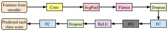
Figure 6.
The architecture of the designed classifier.
Assume the encoder’s output feature map is of size H × W × 128, where H and W denote its spatial height and width, respectively. The detailed parameters and output dimensions of each layer in the classifier were shown in Table 2. The convolutional layer used 64 convolutional kernels of size 3 × 3 × 128 with a stride of 2, reducing the height and width of the input feature map to half of their original size while changing the number of channels to 64. The AvgPool layer reduced the dimension of each feature map by downsampling it to a 1 × 1 feature map. The flatten layer converted the 3D tensor into a 1D tensor with a length of 64. The dropout layer randomly set some neurons to zero with a probability of 0.5 during training to reduce the risk of overfitting, and the output dimension remained 64. The subsequent FC layer, BN layer, ReLU, and dropout layer also had an output dimension of 64. The output dimension of the final FC layer depended on the certain classification task of models: 2 for V-MTL-PlotCounter, 3 for NSPH-MTL-PlotCounter, and 3 for SD-MTL-PlotCounter.
Table 2.
Detailed parameter and output dimension of each layer in the classifier.
2.4.3. Loss Function Construction for MTL-PlotCounter
In multitask driven models, the loss function needs to account for the losses of multiple tasks, including the counting loss and the classification loss. The counting loss, denoted as Loss_count, computed the ℓ1 loss between the predicted count map from the model and the ground truth count map, as presented in Equation (1). The computation of the classification loss involved two steps. First, the scores for each class were converted into probabilities using the softmax function, as presented in Equation (2). Subsequently, the cross-entropy loss function was employed to calculate the classification loss, as presented in Equation (3).
where N is the number of samples, and C represents the number of classes in each classification task. The represents the ground truth count map and represents the predicted count map for the i-th sample, respectively. The represents the predicted score for the i-th sample belonging to the c-th class, and denotes the predicted probability for the i-th sample belonging to the c-th class, respectively. The is the one-hot encoding of the ground truth class label for the i-th sample, which equals 1 if the i-th sample belongs to the c-th class and 0 otherwise.
MTL-PlotCounter adopted a weighted sum approach to construct a loss function suitable for multitask learning. The multitask loss, denoted as MLoss, used a weight of 0.01 to balance the magnitudes of Loss_count and Loss_cls. The MLoss is formulated in Equation (4).
The counting task served as the primary task in MTL-PlotCounter, while the classification task acted as an auxiliary task aimed at driving improvements in counting accuracy. Consequently, MLoss was only used during the training process. During validation, the MAE between the predicted and ground truth plot-scale seedling counts was used to select the optimal model weights suitable for the plot-scale counting task. Given a validation set containing N samples, let denote the predicted seedling count and the corresponding ground truth count for the i-th sample. The MAE is formulated in Equation (5).
2.5. The Design of the Plot-Scale Counting Agent
To facilitate the use of the plot-scale counting model, this study designed and deployed plot-scale counting agents on a web platform, which included both the PlotCounter Agent and the V-MTL-PlotCounter Agent. The core modules of the agent comprised image uploading, plot-scale counting, counting results displaying, and an AI analysis assistant that integrated a multimodal LLM. Technically, the backend employed the FastAPI framework for image uploading and model inference, while the frontend interface was designed using HTML (hypertext markup language) and CSS (cascading style sheets), featuring a green-themed layout. For the multimodal LLM component, the Gemini-2.0-flash model was selected to enable user interaction and intelligent analysis.
The overall framework of the plot-scale counting agent was illustrated in Figure 7. After users uploaded a plot image to the agent, it first retrieved the image dimensions and fed the image into the trained model, either the PlotCounter or V-MTL-PlotCounter. Using the PlotCounter model, the agent inferred the count map and the count result for the plot (predicted plot count). In addition to predicting the count result, the V-MTL-PlotCounter model could also predict the soybean variety of the plot. The agent displayed the count map and count result on the left side of the webpage and included the predicted plot count, variety (unknown for PlotCounter), and plot image size in the image analysis report, which was shown on the right side of the webpage. Subsequently, the agent inputted the original plot image, the image analysis report, and an analysis prompt into the Gemini-2.0-flash model for further analysis of emergence rate and to provide professional advice.
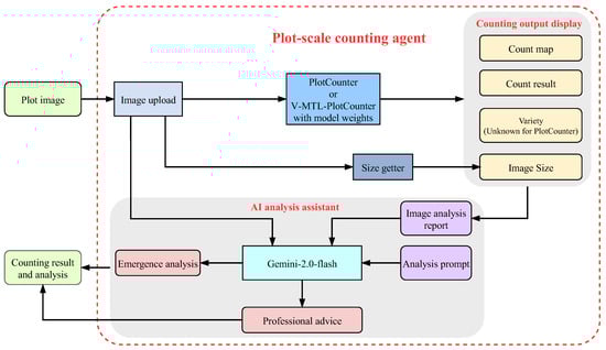
Figure 7.
Overall framework of the plot-scale counting agent.
2.6. Experimental Setting
The experiments were conducted using a laptop featuring a 14-core Intel (R) Core (TM) i7 CPU, 40 GB RAM, 2.28 TB storage, and an NVIDIA RTX 3070 Ti GPU. The operating system utilized was Windows 11, and all models were developed in Python 3.8.3 using PyTorch 1.12. The training was initialized with a learning rate of 0.01, which was reduced ten-fold at both the 200th and 400th epochs during the 500 training epochs. Momentum was configured at 0.95, while a weight decay parameter of 0.0005 was employed.
2.7. Evaluation Metrics
The counting performance of the models was evaluated using MAE, root mean squared error (RMSE), relative MAE (rMAE), relative RMSE (rRMSE), and the coefficient of determination (R2). The corresponding formulas are provided in the following equations.
where N represents the total number of samples, while and represent the ground truth count and predicted count for the i-th sample, respectively. denotes the mean value of all ground truth counts.
The evaluation metric for the model’s classification performance is accuracy, which serves as the most intuitive measure of classification effectiveness. In this study, accuracy was defined task-specifically: for variety classification in V-MTL-PlotCounter, it represented the proportion of correctly identified soybean variety plots; for NSPH classification in NSPH-MTL-PlotCounter, it indicated the proportion of plots with accurately determined NSPH; and for sowing density classification in SD-MTL-PlotCounter, it denoted the proportion of plots with correctly assessed sowing densities.
3. Results
3.1. Comparison of Different Models Employed in PlotCounter
During the experiment, TasselNetV2++ [28], TasselNetV2+ [27], CBAM-TasselNetV2+ [28], and YOLOv5s-Counter [28] were explored as the core models of PlotCounter, respectively. The quantitative evaluation results of plot-scale counting by PlotCounter using different models were shown in Table 3. It can be observed that PlotCounter, using TasselNetV2++ (denoted as PlotCounter), achieved the highest counting accuracy.
Table 3.
Quantitative evaluation results of plot-scale counting by PlotCounter using different models.
Both the single-task and multitask plot soybean seedling counting models generated count maps in the form of grayscale images. To visually demonstrate the counting effects, these grayscale images were converted into color images, resized to match the dimensions of the input plot images, and then overlaid onto the input plot images. Figure 8 presented the visualization of counting outputs generated by the plot-scale counting models.
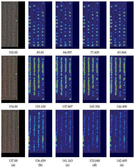
Figure 8.
Visualization of counting outputs generated by the plot-scale counting models. (a) Ground truth. (b) Visualization of count map by PlotCounter. (c) Visualization of count map by PlotCounter using TasselNetV2+. (d) Visualization of count map by PlotCounter using CBAM-TasselNetV2+. (e) Visualization of count map by PlotCounter using YOLOv5s-Counter.
To accurately compare the counting effectiveness of multiple models, including subimage accumulation counting and direct plot-scale counting, the experiments uniformly used plot images with zero-padding edges, which resulted in black borders around the plot images in Figure 8. From Figure 8, it was evident that when counting a plot with three seeds per hole (the first plot depicted in Figure 8), the counting result of each model deviated significantly from the ground truth, while the counting performance of each model was generally good in other cases. Among the samples shown in Figure 8, PlotCounter produced estimates most closely aligned with the ground truth compared to other models. Therefore, TasselNetV2++ was chosen as the core model of PlotCounter.
3.2. Comparison of Subimage Count Accumulation and PlotCounter
Two ways for counting soybean seedlings at the plot scale were compared. One way involved accumulating the counting results of subimages, and the other involved directly counting from plot images. To ensure an accurate comparison between these two ways, the same plot images were used for both. For subimage counting, zero-padding was applied to the edges of the plot images to ensure that each plot image could be evenly divided into 18 subimages. Similarly, zero-padded plot images were also used for direct counting from plot images.
Table 4 presented the quantitative evaluation results of TasselNetV2++ (accumulating the counting results of subimages using TasselNetV2++) and PlotCounter at the plot scale. As shown in Table 4, PlotCounter exhibited superior counting performance across all quantitative evaluation metrics, with an MAE of 5.22, an RMSE of 6.98, an rMAE of 5.22%, an rRMSE of 6.93%, and an R2 of 0.9673, significantly outperforming TasselNetV2++. The superior counting performance of PlotCounter stemmed from its approach to the organization of training samples and the data scale for model validation. PlotCounter adopted a new approach for organizing training samples. Each plot image in the training set was scaled down by a factor of 0.5, and then 20 image patches of 512 × 512 pixels were randomly cropped as training samples. This approach effectively increased the number of samples per training epoch to 600 (i.e., 20 times the number of training plots), addressing the issue of insufficient training samples when the training set contained only 30 plots. In terms of model validation, PlotCounter directly used each plot image in the validation set, fully considering plot-scale information, and selected the optimal weights suitable for the plot-scale counting task.
Table 4.
Quantitative evaluation results of plot-scale counting by TasselNetV2++ and PlotCounter.
3.3. Comparison of PlotCounter and MTL-PlotCounter
To enhance the accuracy of plot-scale counting task, three multitask driven models were designed, including V-MTL-PlotCounter, NSPH-MTL-PlotCounter, and SD-MTL-PlotCounter. Table 5 presented the quantitative evaluation results of plot-scale counting by PlotCounter and MTL-PlotCounter. As shown in Table 5, both PlotCounter and V-MTL-PlotCounter significantly outperformed NSPH-MTL-PlotCounter and SD-MTL-PlotCounter across all counting performance metrics. Comparing V-MTL-PlotCounter with PlotCounter, it was found that V-MTL-PlotCounter achieved relative reductions of 1.92%, 8.74%, 5.17%, and 3.03% in MAE, RMSE, rMAE, and rRMSE metrics, respectively, compared to PlotCounter, while their performances in the R2 metric were comparable. These results indicated that using variety classification as an auxiliary task indeed helped improve the accuracy of plot-scale soybean seedling counting, whereas using NSPH and sowing density classifications as auxiliary tasks did not drive an improvement in counting accuracy.
Table 5.
Quantitative evaluation results of plot-scale counting by PlotCounter and MTL-PlotCounter.
Figure 9 presented the visualization of counting outputs generated by PlotCounter and MTL-PlotCounter on certain test plots. The experiments uniformly utilized plot images with zero-padding on the edges, resulting in plot images with black borders, as shown in Figure 9. From the counting effects shown in Figure 9, it was evident that the plot seedling count predicted by V-MTL-PlotCounter was closer to the ground truth, while the predicted plot seedling counts from NSPH-MTL-PlotCounter and SD-MTL-PlotCounter were relatively similar to those from PlotCounter. Especially in the case of counting plot with three seeds per hole (the first plot in Figure 9), the counting result of V-MTL-PlotCounter was closer to the ground truth than the others, maintaining good performance even in highly occluded scenarios.
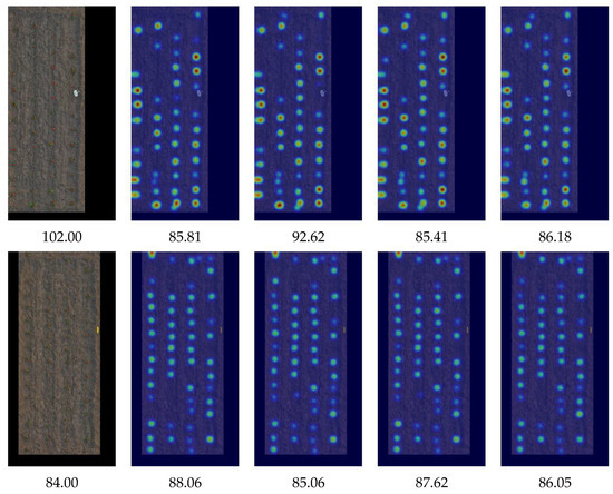
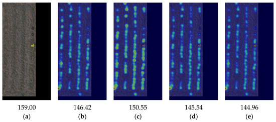
Figure 9.
Visualization of counting outputs generated by PlotCounter and MTL-PlotCounter. (a) Ground truth. (b) PlotCounter’s count map visualization. (c) V-MTL-PlotCounter’s count map visualization. (d) NSPH-MTL-PlotCounter’s count map visualization. (e) SD-MTL-PlotCounter’s count map visualization.
The accuracies of V-MTL-PlotCounter, NSPH-MTL-PlotCounter, and SD-MTL-PlotCounter in their respective classification tasks were 83.33%, 66.67%, and 66.67%, respectively. Due to incomplete seed emergence, the actual NSPH and planting density observed during image data collection may have deviated from the initial sowing settings. The lower classification accuracies for NSPH and sowing density were likely attributed to discrepancies between the actual values during the seedling stage and the labels assigned at the sowing stage. Meanwhile, the soybean varieties remained unchanged in the seedling stage, and the variety classification task achieved relatively good performance.
3.4. The Results of Counting Agents
The feature demonstration of PlotCounter Agent was presented in Figure S1. To use the counting agent, users must upload each plot image separately, rather than the entire map of the experimental field. When a plot image was uploaded into the PlotCounter Agent, it displayed the count map and result, as shown in Figure S1a. Since PlotCounter cannot predict the variety category, the image analysis report showed “Variety: unknown”. The report also displayed the spatial size of the plot image and the predicted seedling count. When the sown seeds, manual seedling count, and prompt for analyzing actual and predicted emergence rates were inputted, as illustrated in Figure S1b, the multimodal LLM component combined the information from the image analysis report and original plot image to provide emergence analysis. Emergence analysis from PlotCounter Agent was shown in Figure S1c.
The feature demonstration of the V-MTL-PlotCounter Agent was shown in Figure S2. Compared to PlotCounter Agent, V-MTL-PlotCounter Agent can also predict the variety category, as demonstrated in Figure S2a, where it predicted the variety of the plot as “Dongdou 1”. Additionally, the agent offered a “Generate Analysis Prompt” function. By clicking the “Generate Analysis Prompt” button, users can select information such as variety, soil, and field management and choose the analysis direction, as shown in Figure S2b, to automatically generate the analysis prompt. The automatically generated analysis prompt was depicted in Figure S2c. Breeders can input the soybean seedling image of a plot directly through the web platform to obtain a counting result, predict seedling count, analyze emergence rate using either the PlotCounter Agent or V-MTL-PlotCounter Agent, and conduct interactive analysis with prompts based on the multimodal LLM.
4. Discussion
4.1. The Outset of PlotCounter
Based on discussions with agricultural breeding experts and a review of recent studies [45], it is clear that the emergence rate at the plot scale is the primary concern in breeding trials, rather than the seedling count in individual subimages. To address this practical requirement, the UAV mosaic image was divided according to plots, and an end-to-end soybean seedling counting model at the plot scale, called PlotCounter, was proposed. This model allows for the acquisition of the total number of seedlings in a plot simply by inputting the plot image.
The PlotCounter adopted a new organization form of samples to address the issue of insufficient training samples at the plot scale and used entire plot images during the model validation process to select the optimal weights suitable for the plot-scale counting task, thereby significantly improving the counting accuracy of soybean seedlings at the plot scale. As stated by Farjon and Edan [46], correct data augmentation strategies, systematic dataset partitioning, and reasonable image patching methods are crucial for enhancing model performance. For practical application scenarios, adopting a dataset partitioning method along with a reasonable organization of training samples and validation scale tailored to the specific task is an effective strategy for improving accuracy. This approach may be more efficient than modifying the model itself.
4.2. The Counting Effect of V-MTL-PlotCounter
To demonstrate the counting efficacy of V-MTL-PlotCounter, we compared it with PlotCounter and state-of-the-art detection-based counting models, including YOLOv5s [40], YOLOv7 [26], and YOLOv8s [23], at the plot scale in terms of counting accuracy. The quantitative evaluation results of plot-scale counting by various models were presented in Table 6. It can be observed that V-MTL-PlotCounter outperformed the other models in counting accuracy metrics such as MAE, RMSE, rMAE, and rRMSE, achieving a comparable R2 to PlotCounter. It is worth noting that PlotCounter and MTL-PlotCounter adopted a patch-based training strategy combined with full-plot validation, which allowed for direct inference on full-plot images to obtain plot-scale seedling counts. In contrast, YOLOv5s, YOLOv7, and YOLOv8s generated plot-scale predictions by aggregating the counts from their subimage-scale outputs.
Table 6.
Quantitative evaluation results of plot-scale counting by various counting models.
For an intuitive comparison of the overall counting accuracy across various models at the plot scale, Figure 10 presented a radar chart with five axes representing MAE, RMSE, rMAE, rRMSE, and R2. To better visualize performance differences among models, each axis of the radar chart was scaled by setting the maximum to the best performance, extending outward by one-tenth of the range between the best and worst values, and the minimum to the worst performance, extending inward by the same proportion. Upon examining the radar chart, it became apparent that the proposed V-MTL-PlotCounter exhibited superior counting performance at the plot scale compared to these models.
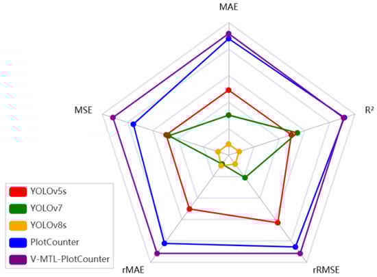
Figure 10.
Radar chart comparing the counting performance of various counting models.
The YOLO series was selected as the state-of-the-art comparison model for two main reasons. It is widely used as the benchmark in recent counting studies, and one branch of the encoder in the proposed models incorporates a customized YOLOv5s backbone. Each model has its own strengths depending on the application scenario. The YOLO models are well recognized for their practicality and versatility in object detection tasks, but they are not end-to-end counting models, as their final counts are derived from detection results. In contrast, the proposed PlotCounter directly estimates the number of seedlings per plot, making it particularly suitable for breeding plot scenarios. With sufficient data across different varieties, V-MTL-PlotCounter can simultaneously perform variety classification and seedling counting, demonstrating strong potential for broader applications.
To evaluate the robustness of V-MTL-PlotCounter against variations in UAV image color characteristics, the model was tested on images with adjusted brightness, contrast, saturation, hue, and color temperature, including slight, moderate, and large levels of change. As shown in Table 7, the model maintained stable accuracy under slight and moderate adjustments, while performance declined under large shifts. These results indicate that the model is generally robust to common color variations. In future deployments, integrating a color correction module into the counting agent could further improve adaptability to diverse UAV imaging conditions.
Table 7.
Performance of V-MTL-PlotCounter under different color adjustments.
4.3. The Application Prospect of the Plot-Scale Counting Agent
Breeders can input plot images into the PlotCounter Agent via a web platform to obtain the total number of seedlings in the plot, significantly facilitating breeding efforts. Additionally, by leveraging the multimodal LLM, the PlotCounter Agent can analyze the emergence rate by inputting the actual sowing parameters for the plot. In the future, when the variety of collected soybean data becomes sufficiently diverse, images can be fed into the V-MTL-PlotCounter Agent to simultaneously predict the total seedling count and soybean variety. The V-MTL-PlotCounter Agent, which integrated seedling counting, variety identification, and intelligent analysis, greatly enhanced the efficiency of obtaining the plot information.
4.4. Current Limitations and Insights for Future Studies
The primary limitation of this study lies in the use of a limited number of plots and soybean varieties, with only 54 in total collected from a single site within a single year, which inevitably imposed constraints on both the model’s performance and its generalizability to broader field conditions. To train the deep learning model with the available 54 plot images, an innovative sample organization strategy was employed due to the use of the regression-based counting model, which accommodated scale differences between validation and training samples compared with others. While the current limitations in plot variety and diversity may restrict generalizability, the developed model offered a viable solution for deep learning applications in small sample scenarios, achieving an accuracy level suitable for practical plot-scale counting. As data from multiple soybean varieties and diverse field environments become available in future studies, the model’s plot-scale counting accuracy is expected to improve further.
The motivation behind jointly optimizing classification and counting as dual tasks during training was the significant impact that different varieties and sowing methods have on emergence. Multitask learning was used to associate these effects and optimize multitask accordingly. Among the three MTL-PlotCounter models, only V-MTL-PlotCounter demonstrated an improvement in counting accuracy. During UAV image acquisition, due to incomplete seed emergence, only the soybean variety remained consistent with the initial sowing settings in each plot, while the NSPH and planting density values deviated. The experiments showed that using accurate and relevant information prediction as an auxiliary task can effectively enhance the main task’s performance.
Although RGB imagery is widely used in breeding trials due to its accessibility and low cost [17,18], future extensions of this work could benefit from incorporating multispectral and Light Detection and Ranging (LiDAR) data. Multispectral imagery enables the calculation of diverse vegetation indices and improves crop segmentation by including near-infrared spectral information [13,47]. LiDAR, in contrast, provides detailed three-dimensional canopy structure and height measurements [48,49]. With accurate geospatial alignment, these complementary data sources could be integrated into the proposed multitask learning framework to enable simultaneous seedling counting, variety identification, and phenological stage estimation [50].
The proposed V-MTL-PlotCounter, deployed as an interactive agent on a web platform, enables automated soybean variety identification, seedling counting, and emergence rate analysis powered by a multimodal LLM. Future work will focus on improving the model’s generalization by incorporating data from diverse crop varieties and enhancing its robustness across varying field environments. Once adapted for seedling counting in multiple crop species, the model will allow agricultural researchers to directly input UAV imagery of breeding plots, facilitating rapid and labor-efficient crop identification and seedling counting.
5. Conclusions
In this study, we constructed a specialized plot-scale dataset, tailored for breeding plot scenarios, which comprises UAV-captured soybean seedling imagery and key sowing-related metadata, including variety, number of seeds per hole, and sowing density, all of which are closely related to plot-scale emergence rate. Using this dataset, we developed PlotCounter, a plot-scale counting model built on the TasselNetV2++ architecture. Leveraging the patch-based training and full-plot validation strategy, PlotCounter achieved accurate seedling counting even under limited data conditions. To further enhance prediction accuracy, we proposed the MTL-PlotCounter framework by incorporating auxiliary classification tasks through multitask learning. Among its variants, V-MTL-PlotCounter, which integrates soybean variety information, demonstrated the best performance, achieving relative reductions of 8.74% in RMSE and 5.17% in rMAE over PlotCounter. It also outperformed models such as YOLOv5s, YOLOv7, and YOLOv8s in plot-scale counting tasks. Both PlotCounter and V-MTL-PlotCounter were deployed as interactive agents on a web platform, enabling breeders to upload plot images, automatically count seedlings, analyze emergence rates, and perform prompt-driven interaction through a multimodal LLM. This study demonstrates the potential of integrating UAV remote sensing, agronomic data, specialized models, and multimodal large language models to enable intelligent crop phenotyping. In future work, we will focus on enhancing model generalization through multiple varieties of data and improving robustness across diverse field environments.
Supplementary Materials
The following supporting information can be downloaded at: https://www.mdpi.com/article/10.3390/rs17152688/s1. Figure S1: Feature demonstration of PlotCounter Agent. (a) Counting result of PlotCounter Agent. (b) Emergence analysis prompt. (c) Emergence analysis of PlotCounter Agent. Figure S2: Feature demonstration of V-MTL-PlotCounter Agent. (a) Counting and variety classification results of V-MTL-PlotCounter Agent. (b) Analysis prompt generation process. (c) Automatically generated analysis prompt.
Author Contributions
Conceptualization, H.S.; methodology, X.X. and H.S.; software, X.X. and C.L.; validation, Z.L. and Y.S.; formal analysis, H.S. and X.L.; investigation, Z.L. and X.L.; resources, H.S. and X.X.; data curation, C.L. and Y.S.; writing—original draft preparation, X.X.; writing—review and editing, H.S.; visualization, X.X. and C.L.; supervision, H.S.; project administration, H.S.; funding acquisition, H.S., X.X. and X.L. All authors have read and agreed to the published version of the manuscript.
Funding
This research was funded by the National Key Research and Development Program of China, grant number 2021YFD1600602-09 and Basic Research Project of Shanxi Province (Youth), grant number 202303021222067, 202203021212455.
Data Availability Statement
The original data presented in the study are openly available in [V-MTL-PlotCounter-Agent] at [https://github.com/2xuexiao/V-MTL-PlotCounter-Agent] (accessed on 31 July 2025).
Conflicts of Interest
The authors declare no conflicts of interest.
Abbreviations
The following abbreviations are used in this manuscript:
| UAV | Unmanned Aerial Vehicle |
| FCN | Fully Convolutional Network |
| MTL | Multitask Learning |
| LLM | Large Language Model |
| AI | Artificial Intelligence |
| NSPH | Numbers of Seeds Per Hole |
| GD | Gathering and Distribution |
| AvgPool | Average Pooling |
| Low-IFM | Low-stage Information Fusion Module |
| CBAM | Convolutional Block Attention Module |
| PlotCounter | Plot-scale Counting |
| MTL-PlotCounter | Multitask Driven Plot-scale Counting |
| MAE | Mean Absolute Error |
| V-MTL-PlotCounter | Variety Driven MTL-PlotCounter |
| NSPH-MTL-PlotCounter | NSPH Driven MTL-PlotCounter |
| SD-MTL-PlotCounter | Sowing Density Driven MTL-PlotCounter |
| FC | Fully Connected |
| BN | Batch Normalization |
| ReLU | Rectified Linear Unit |
| HTML | HyperText Markup Language |
| CSS | Cascading Style Sheets |
| RMSE | Root Mean Squared Error |
| rMAE | relative Mean Absolute Error |
| rRMSE | relative Root Mean Squared Error |
| R2 | Coefficient of Determination |
| LiDAR | Light Detection and Ranging |
References
- Graham, P.H.; Vance, C.P. Legumes: Importance and constraints to greater use. Plant Physiol. 2003, 131, 872–877. [Google Scholar] [CrossRef]
- Yang, H.; Fei, L.; Wu, G.; Deng, L.; Han, Z.; Shi, H.; Li, S. A novel deep learning framework for identifying soybean salt stress levels using RGB leaf images. Ind. Crops Prod. 2025, 228, 120874. [Google Scholar] [CrossRef]
- Cox, W.J.; Cherney, J.H. Growth and yield responses of soybean to row spacing and seeding rate. Agron. J. 2011, 103, 123–128. [Google Scholar] [CrossRef]
- Liu, T.; Wu, W.; Chen, W.; Sun, C.; Zhu, X.; Guo, W. Automated image-processing for counting seedlings in a wheat field. Precis. Agric. 2016, 17, 392–406. [Google Scholar] [CrossRef]
- Gnädinger, F.; Schmidhalter, U. Digital counts of maize plants by unmanned aerial vehicles (UAVs). Remote Sens. 2017, 9, 544. [Google Scholar] [CrossRef]
- Koh, J.C.O.; Hayden, M.; Daetwyler, H.; Kant, S. Estimation of crop plant density at early mixed growth stages using UAV imagery. Plant Methods 2019, 15, 64. [Google Scholar] [CrossRef] [PubMed]
- Liu, S.; Yin, D.; Feng, H.; Li, Z.; Xu, X.; Shi, L.; Jin, X. Estimating maize seedling number with UAV RGB images and advanced image processing methods. Precis. Agric. 2022, 23, 1604–1632. [Google Scholar] [CrossRef]
- Dadrass Javan, F.; Samadzadegan, F.; Toosi, A.; van der Meijde, M. Unmanned aerial geophysical remote sensing: A systematic review. Remote Sens. 2025, 17, 110. [Google Scholar] [CrossRef]
- Pathak, H.; Igathinathane, C.; Zhang, Z.; Archer, D.; Hendrickson, J. A review of unmanned aerial vehicle-based methods for plant stand count evaluation in row crops. Comput. Electron. Agric. 2022, 198, 107064. [Google Scholar] [CrossRef]
- Ludwig, M.; Runge, C.M.; Friess, N.; Koch, T.L.; Richter, S.; Seyfried, S.; Wraase, L.; Lobo, A.; Sebastià, M.-T.; Reudenbach, C.; et al. Quality assessment of photogrammetric methods—A workflow for reproducible UAS orthomosaics. Remote Sens. 2020, 12, 3831. [Google Scholar] [CrossRef]
- Olson, D.; Anderson, J. Review on unmanned aerial vehicles, remote sensors, imagery processing, and their applications in agriculture. Agron. J. 2021, 113, 971–992. [Google Scholar] [CrossRef]
- Gao, M.; Yang, F.; Wei, H.; Liu, X. Automatic monitoring of maize seedling growth using unmanned aerial vehicle-based RGB imagery. Remote Sens. 2023, 15, 3671. [Google Scholar] [CrossRef]
- Feng, Y.; Chen, W.; Ma, Y.; Zhang, Z.; Gao, P.; Lv, X. Cotton seedling detection and counting based on UAV multispectral images and deep learning methods. Remote Sens. 2023, 15, 2680. [Google Scholar] [CrossRef]
- Feng, A.; Zhou, J.; Vories, E.; Sudduth, K.A. Evaluation of cotton emergence using UAV-based narrow-band spectral imagery with customized image alignment and stitching algorithms. Remote Sens. 2020, 12, 1764. [Google Scholar] [CrossRef]
- Jiang, Y.; Li, C. Convolutional neural networks for image-based high-throughput plant phenotyping: A review. Plant Phenomics 2020, 2020, 4152816. [Google Scholar] [CrossRef] [PubMed]
- Huang, Y.; Qian, Y.; Wei, H.; Lu, Y.; Ling, B.; Qin, Y. A survey of deep learning-based object detection methods in crop counting. Comput. Electron. Agric. 2023, 215, 108425. [Google Scholar] [CrossRef]
- Diez, Y.; Kentsch, S.; Fukuda, M.; Caceres, M.L.L.; Moritake, K.; Cabezas, M. Deep learning in forestry using UAV-acquired RGB data: A practical review. Remote Sens. 2021, 13, 2837. [Google Scholar] [CrossRef]
- Gano, B.; Bhadra, S.; Vilbig, J.M.; Ahmed, N.; Sagan, V.; Shakoor, N. Drone-based imaging sensors, techniques, and applications in plant phenotyping for crop breeding: A comprehensive review. Plant Phenome J. 2024, 7, e20100. [Google Scholar] [CrossRef]
- Oh, S.; Chang, A.; Ashapure, A.; Jung, J.; Dube, N.; Maeda, M.; Gonzalez, D.; Landivar, J. Plant counting of cotton from UAS imagery using deep learning-based object detection framework. Remote Sens. 2020, 12, 2981. [Google Scholar] [CrossRef]
- Redmon, J.; Farhadi, A. YOLOv3: An incremental improvement. arXiv 2018, arXiv:1804.02767. [Google Scholar] [CrossRef]
- Barreto, A.; Lottes, P.; Ispizua Yamati, F.R.; Baumgarten, S.; Wolf, N.A.; Stachniss, C.; Mahlein, A.; Paulus, S. Automatic UAV-based counting of seedlings in sugar-beet field and extension to maize and strawberry. Comput. Electron. Agric. 2021, 191, 106493. [Google Scholar] [CrossRef]
- Chen, X.; Liu, T.; Han, K.; Jin, X.; Wang, J.; Kong, X.; Yu, J. TSP-yolo-based deep learning method for monitoring cabbage seedling emergence. Eur. J. Agron. 2024, 157, 127191. [Google Scholar] [CrossRef]
- Ultralytics YOLOv8. Available online: https://github.com/ultralytics/ultralytics (accessed on 20 December 2024).
- Shahid, R.; Qureshi, W.S.; Khan, U.S.; Munir, A.; Zeb, A.; Moazzam, S. Aerial imagery-based tobacco plant counting framework for efficient crop emergence estimation. Comput. Electron. Agric. 2024, 217, 108557. [Google Scholar] [CrossRef]
- Ronneberger, O.; Fischer, P.; Brox, T. U-Net: Convolutional networks for biomedical image segmentation. In Proceedings of the International Conference on Medical Image Computing and Computer-Assisted Intervention (MICCAI), Munich, Germany, 5–9 October 2015; pp. 234–241. [Google Scholar] [CrossRef]
- Wang, C.; Bochkovskiy, A.; Liao, H. YOLOv7: Trainable bag-of-freebies sets new state-of-the-art for real-time object detectors. In Proceedings of the IEEE/CVF Conference on Computer Vision and Pattern Recognition (CVPR), Vancouver, BC, Canada, 18–22 June 2023; pp. 7464–7475. [Google Scholar] [CrossRef]
- Lu, H.; Cao, Z. TasselNetV2+: A fast implementation for high-throughput plant counting from high-resolution RGB imagery. Front. Plant Sci. 2020, 11, 541960. [Google Scholar] [CrossRef]
- Xue, X.; Niu, W.; Huang, J.; Kang, Z.; Hu, F.; Zheng, D.; Wu, Z.; Song, H. TasselNetV2++: A dual-branch network incorporating branch-level transfer learning and multilayer fusion for plant counting. Comput. Electron. Agric. 2024, 223, 109103. [Google Scholar] [CrossRef]
- De Souza, F.L.P.; Shiratsuchi, L.S.; Dias, M.A.; Júnior, M.R.B.; Setiyono, T.D.; Campos, S.; Tao, H. A neural network approach employed to classify soybean plants using multi-sensor images. Precis. Agric. 2025, 26, 32. [Google Scholar] [CrossRef]
- Zhang, Y.; Yang, Q. A survey on multi-task learning. IEEE Trans. Knowl. Data Eng. 2021, 34, 5586–5609. [Google Scholar] [CrossRef]
- Lin, Z.; Zhong, R.; Xiong, X.; Guo, C.; Xu, J.; Zhu, Y.; Xu, J.; Ying, Y.; Ting, K.C.; Huang, J.; et al. Large-scale rice mapping using multi-task spatiotemporal deep learning and Sentinel-1 SAR time series. Remote Sens. 2022, 14, 699. [Google Scholar] [CrossRef]
- Pound, M.P.; Atkinson, J.A.; Wells, D.M.; Pridmore, T.P.; French, A.P. Deep learning for multi-task plant phenotyping. In Proceedings of the IEEE International Conference on Computer Vision Workshops (ICCV), Venice, Italy, 22–29 October 2017; pp. 2055–2063. [Google Scholar] [CrossRef]
- Dobrescu, A.; Giuffrida, M.V.; Tsaftaris, S.A. Doing more with less: A multitask deep learning approach in plant phenotyping. Front. Plant Sci. 2020, 11, 141. [Google Scholar] [CrossRef]
- Jiao, L.; Liu, Q.; Liu, H.; Chen, P.; Wang, R.; Liu, K.; Dong, S. WheatNet: Attentional path aggregation feature pyramid network for precise detection and counting of dense and arbitrary-oriented wheat spikes. IEEE Trans. AgriFood Electron. 2024, 2, 606–616. [Google Scholar] [CrossRef]
- Ge, Z.; Liu, S.T.; Wang, F.; Li, Z.; Sun, J. YOLOX: Exceeding YOLO series in 2021. arXiv 2021, arXiv:2107.08430. [Google Scholar] [CrossRef]
- Li, Y.; Yang, J. Few-shot cotton pest recognition and terminal realization. Comput. Electron. Agric. 2020, 169, 105240. [Google Scholar] [CrossRef]
- Sun, J.; Ren, Z.; Cui, J.; Tang, C.; Luo, T.; Yang, W.; Song, P. A high-throughput method for accurate extraction of intact rice panicle traits. Plant Phenomics 2024, 6, 0213. [Google Scholar] [CrossRef] [PubMed]
- Gu, Z.; He, D.; Huang, J.; Chen, J.; Wu, X.; Huang, B.; Dong, T.; Yang, Q.; Li, H. Simultaneous detection of fruits and fruiting stems in mango using improved YOLOv8 model deployed by edge device. Comput. Electron. Agric. 2024, 227, 109512. [Google Scholar] [CrossRef]
- Xu, W.; Yang, R.; Karthikeyan, R.; Shi, Y.; Su, Q. GBiDC-PEST: A novel lightweight model for real-time multiclass tiny pest detection and mobile platform deployment. J. Integr. Agric. 2024, in press. [Google Scholar] [CrossRef]
- Ultralytics YOLOv5. Available online: https://github.com/ultralytics/yolov5 (accessed on 20 December 2024).
- Kuska, M.T.; Wahabzada, M.; Paulus, S. AI for crop production—Where can large language models (LLMs) provide substantial value? Comput. Electron. Agric. 2024, 221, 108924. [Google Scholar] [CrossRef]
- Zhu, H.; Shi, W.; Guo, X.; Lyu, S.; Yang, R.; Han, Z. Potato disease detection and prevention using multimodal AI and large language model. Comput. Electron. Agric. 2025, 229, 109824. [Google Scholar] [CrossRef]
- Wang, C.; He, W.; Nie, Y.; Guo, J.; Liu, C.; Han, K.; Wang, Y. Gold-YOLO: Efficient object detector via gather-and-distribute mechanism. arXiv 2023, arXiv:2309.11331. [Google Scholar] [CrossRef]
- Woo, S.; Park, J.; Lee, J.Y.; Kweon, I.S. CBAM: Convolutional block attention module. In Proceedings of the European Conference on Computer Vision (ECCV), Munich, Germany, 8–14 September 2018; pp. 3–19. [Google Scholar] [CrossRef]
- Sun, Y.; Li, M.; Liu, M.; Zhang, J.; Cao, Y.; Ao, X. A statistical method for high-throughput emergence rate calculation for soybean breeding plots based on field phenotypic characteristics. Plant Methods 2025, 21, 40. [Google Scholar] [CrossRef]
- Farjon, G.; Edan, Y. AgroCounters—A repository for counting objects in images in the agricultural domain by using deep-learning algorithms: Framework and evaluation. Comput. Electron. Agric. 2024, 222, 108988. [Google Scholar] [CrossRef]
- Zheng, H.; Zhou, X.; He, J.; Yao, X.; Cheng, T.; Zhu, Y.; Cao, W.; Tian, Y. Early season detection of rice plants using RGB, NIR-G-B and multispectral images from unmanned aerial vehicle (UAV). Comput. Electron. Agric. 2020, 169, 105223. [Google Scholar] [CrossRef]
- Maesano, M.; Khoury, S.; Nakhle, F.; Firrincieli, A.; Gay, A.; Tauro, F.; Harfouche, A. UAV-based LiDAR for high-throughput determination of plant height and above-ground biomass of the bioenergy grass Arundo donax. Remote Sens. 2020, 12, 3464. [Google Scholar] [CrossRef]
- Rivera, G.; Porras, R.; Florencia, R.; Sánchez-Solís, J.P. LiDAR applications in precision agriculture for cultivating crops: A review of recent advances. Comput. Electron. Agric. 2023, 207, 107737. [Google Scholar] [CrossRef]
- Kleinsmann, J.; Verbesselt, J.; Kooistra, L. Monitoring individual tree phenology in a multi-species forest using high resolution UAV images. Remote Sens. 2023, 15, 3599. [Google Scholar] [CrossRef]
Disclaimer/Publisher’s Note: The statements, opinions and data contained in all publications are solely those of the individual author(s) and contributor(s) and not of MDPI and/or the editor(s). MDPI and/or the editor(s) disclaim responsibility for any injury to people or property resulting from any ideas, methods, instructions or products referred to in the content. |
© 2025 by the authors. Licensee MDPI, Basel, Switzerland. This article is an open access article distributed under the terms and conditions of the Creative Commons Attribution (CC BY) license (https://creativecommons.org/licenses/by/4.0/).