Estimating Household Green Space in Composite Residential Community Solely Using Drone Oblique Photography

Abstract

Residential green space is an important component of urban green space and one of the major indicators for evaluating the quality of a residential community. Traditional indicators such as the green space ratio only consider the relationship between green space area and total area of the residential community while ignoring the difference in the amount of green space enjoyed by household residents in high-rise and low-rise buildings. Therefore, it is meaningful to estimate household green space and its spatial distribution in residential communities. However, there are frequent difficulties in obtaining specific green space area and household number through ground surveys or consulting with property management units. In this study, taking a composite residential community in Chongqing, China, as the study site, we first employed a five-lens drone to capture its oblique RGB images and generated the DOM (Digital Orthophoto Map). Subsequently, the green space area and distribution in the entire residential community were extracted from the DOM using VDVI (Visible Difference Vegetation Index). The YOLACT (You Only Look At Coefficients) instance segmentation model was used to recognize balconies from the facade images of high-rise buildings to determine their household numbers. Finally, the average green space per household in the entire residential community was calculated to be 67.82 m², and those in the high-rise and low-rise building zones were 51.28 m² and 300 m², respectively. Compared with the green space ratios of 65.5% and 50%, household green space more truly reflected the actual green space occupation in high- and low-rise building zones.

1. Introduction

UGS (urban green space) can provide necessary ecological and environmental services [1], such as reducing urban heat island effects [2], enhancing biodiversity [3], and improving air quality [4], which are crucial for sustainable urbanization and human well-being [5]. RGS (residential green space), as one of the six types of UGSs, plays an important role. RGS usually includes public green spaces within a residential community and green spaces around buildings, which are closely related to the daily lives of residents. High-quality RGS can promote the physical activities of residents [6], improve their physical and mental health, and enhance their satisfaction with the residential community [7]. Therefore, RGS is one of the major factors deciding the quality of a residential community.

The area of RGS is the most fundamental information of a residential community, which is usually achieved via green space surveys. Accurate green space data help planners optimize the allocation of green resources, formulate strategies to improve the overall green situation, and promote fair access of green space resources [8]. Early green space surveys mainly used a combination of manual surveys and mathematical statistical analysis, which required a great amount of manpower and material resources, and the obtained data had the disadvantage of subjectivity [9]. With the development of remote sensing technology, remote sensing-based surveys have gradually become the mainstream of green space survey methods, with the advantages of strong timeliness and low cost [10]. However, green spaces in residential communities commonly exhibit high fragmentation and heterogeneity, so it is difficult to accurately extract them from satellite remotely sensed images of relatively low resolutions [11]. Usually, it requires a large amount of ground surveys to supplement, which cannot satisfy the automation and intelligence requirements of modern urban green space surveys. The combination of drone oblique photography and deep learning methods provides a new solution to this issue and plays an increasingly important role in smart cities [12]. Compared with satellite remote sensing, drone oblique photography has the characteristics of high flexibility, high resolution, and multi-angle photography [13]. The multi-angle photography can obtain facade images of the buildings, which will provide detailed side building information and even be used to produce the DSM (Digital Surface Model) of the entire residential communities.

As an indicator for quantifying vegetation coverage and growth status, the vegetation index is widely used to extract green spaces from remotely sensed data [14]. It usually enhances certain features and details of vegetation by combining the reflectance values of two or more bands. Currently, over a hundred vegetation indices have been proposed, including NDVI (Normalized Difference Vegetation Index) [15], EVI (Enhanced Vegetation Index) [16], and RVI (Ratio Vegetation Index) [17]. These widely used vegetation indices commonly utilize both visible and near-infrared spectral bands, which are very sensitive to vegetation. However, most drones are equipped with consumer-grade cameras and do not have near-infrared bands. Therefore, researchers attempted to construct vegetation indices using only RGB (red, green, and blue) bands, such as EXG (Excess Green) [18], CIVE (Color Index for Vegetation Extraction) [19], EXGR (Excess Green minutes Excess Red Difference Index) [20], NGBDI (Normalized Green Blue Difference Index) [21], NGRDI (Normalized Green Red Difference Index) [22], and VDVI (Visible band difference vegetation index) [23]. Yuan et al. [24] found that VDVI performed the best among various RGB vegetation indices in extracting healthy green vegetation from drone-acquired RGB images. At present, the majority of RGB vegetation indices are focused on agricultural land covers and are rarely constructed specifically for urban green space extraction.

The green space ratio is a traditional indicator for RGS evaluation, which refers to the proportion of green space area within a given region. With the emergence of numerous high-rise buildings in modern cities, the population density in residential communities has sharply increased. Due to the neglect of the differences in green space enjoyed by residents in high- and low-rise buildings, the green space ratio is increasingly unable to adapt to the evaluation of green space quality in modern cities. The green area per capita and green plot ratio [25] are two indicators considering the population and building floors in a residential community. But they usually require accurate data of total population and total building area, which cannot be directly obtained from remotely sensed images. Although the property management departments of residential communities usually have access to these two types of data, it is frequently difficult to obtain them due to privacy concerns. In contrast, it is relatively easier to obtain the household number in residential communities with high buildings from remotely sensed data. The average green space per household can more intuitively reflect the different accessibilities of green spaces for residents in buildings on different floors, making it a more practical indicator for RGS evaluation in modern residential communities than the green space ratio.

The building extraction from remotely sensed images is one of the important fields of remote sensing applications [26]. With the emergence of high-resolution remotely sensed data, it has brought new opportunities and challenges for automatically extracting buildings [27]. Due to the limitations in spatial resolution and vertical angle of view, building information extracted from satellite remotely sensed images mainly consists of overall structures rather than detailed features. In contrast, drone oblique photography can obtain facade images of buildings with ultra-high resolution, which can be used to extract building components such as balconies and windows on the side of high-rise buildings. The household number can be further determined according to the correspondence between components and each household. The traditional methods of extracting building components are usually based on image features such as texture and spectrum. As building components generally show morphological diversities in different regions and color variations under different lighting and shadows, the generalization abilities of these methods are typically poor [28].

Deep learning can effectively learn general patterns from large amounts of building component samples and has become the mainstream technology for the intelligent extraction of building components from remotely sensed images [29]. Instance segmentation, as one key technology in the field of computer vision, can accurately identify and segment each independent object in an image and has been widely used for building extraction. For example, Wu et al. [30] applied an improved Anchor-Free Instance Segmentation algorithm to extract buildings from high-resolution remotely sensed images; Chen et al. [31] converted the semantic segmentation results into instances to extract the location and quantity of buildings. Instance segmentation can be seen as a combination of object detection and semantic segmentation. Object detection outputs object bounding boxes and category information, while instance segmentation further classifies pixels within the bounding boxes and outputs mask information of the objects, obtaining more accurate object shapes and numbers. This enables instance segmentation to be used for automatic recognition and counting of building components [32]. For example, Lu et al. [33] applied the SOLOv2 algorithm to accurately segment windows on building facades to obtain the area ratio of windows to building facades, which is the key parameter for simulating and renovating the energy consumption of existing buildings.

Instance segmentation models are mainly divided into two-stage and single-stage models. The two-stage model represented by Mask R-CNN [34] has accurate segmentation results, but its execution speed is relatively slow; the single-stage model is relatively fast and can meet the needs of rapid object recognition. YOLACT (You Only Look At Coefficients) [35] is a real-time single-stage model that achieves accurate instance segmentation by predicting a set of prototype masks and corresponding mask coefficients. Compared to the two-stage models, YOLACT has a significant advantage in speed, while maintaining relatively high accuracy, strong generalization ability, and robustness, making it an ideal choice for identifying the target building components from the facade images of high-rise buildings.

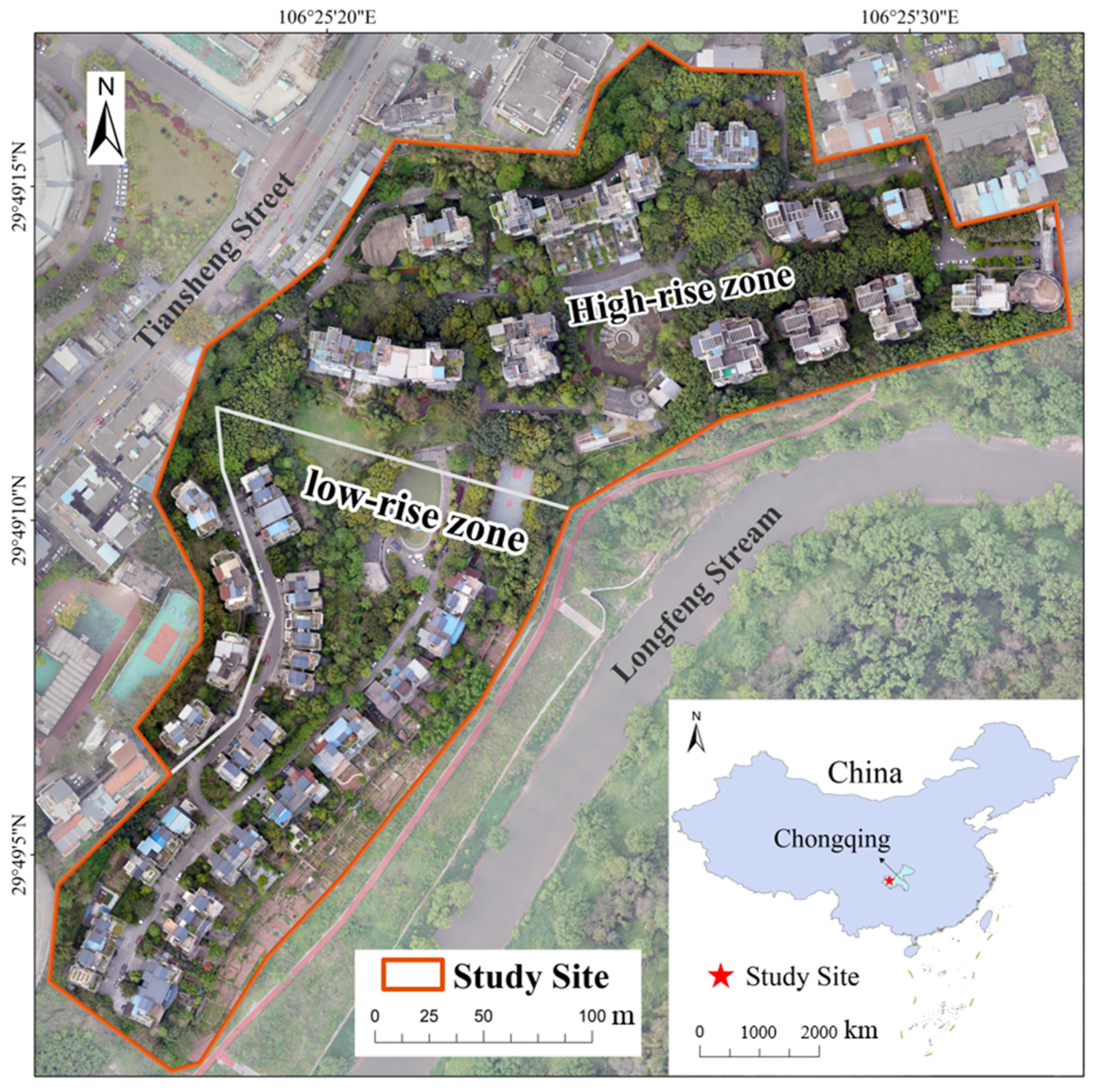
In this study, a composite residential community in Chongqing, China, was taken as the study site, and its oblique RGB images were captured using a five-lens drone. Based on these images, the green space and household number were obtained, and the average green space per household in different building zones was separately calculated. The major objectives include (1) to extract green space using the VDVI vegetation index from the DOM (Digital Orthophoto Map) of the residential community; (2) to obtain the household number of high-rise buildings by automatically recognizing balconies from the facade images using the YOLACT model; (3) to calculate average green space per household in high- and low-rise building zones and analyze the implication for green space evaluation in modern residential communities.

2. Study Site and Data

2.1. Study Site

As indicated in Figure 1, the Panxi Mingdu residential community (106°25′10″–106°25′40”E and 29°49′00″–29°49′20″N) located in Beibei District, Chongqing, China, was selected as the study site, with an elevation ranging from 200 m to 245 m. The residential community covers an area of approximately 0.085 km², with Tiansheng Road crossing above and Longfeng River flowing below. The region belongs to a subtropical humid climate, controlled by the Southeast Asian monsoon circulation, with a mean annual temperature of 18.2 °C and a mean annual precipitation of 1156.8 mm. It has the characteristics of weak wind, high humidity, misty clouds, short sunshine hours, and rare ice and snow.

The residential community is roughly divided into two parts, high-rise building zone and low-rise building zone, with a total of 28 buildings. Among them, there are 16 buildings in the high-rise zone and 12 buildings in the low-rise zone, occupying areas of 0.055 km² and 0.030 km², respectively. Overall, the vegetation types are rich and concentrated, including trees, shrubs, and herbaceous layers. There is a well-developed road network around the community. The convenient transportation and complete supporting facilities can meet the daily needs of the residents. As an old residential community, Panxi Mingdu has a typical and representative level of greenery and architectural composition. Therefore, it is an appropriate study site for studying and estimating household green space in a composite residential community solely using drone oblique photography.

2.2. Drone-Acquired Images

In this study, a quad-rotor drone, Feima D2000 (Feima Robotics, Shenzhen, China), was used for image acquisition, which was equipped with a D-OP5000 (Feima Robotics, Shenzhen, China) five-lens sensor for oblique photography. The image capture for the Panxi Mingdu community was conducted on 2 May 2024. The operation time was between 11:00 a.m. and 1:00 p.m. during the sunny period, when the high surface reflectance was beneficial to acquire high-quality images. The flight altitude was set to 120 m, and the lateral and heading overlap rates were 75% and 80%, respectively. A belt-shaped trajectory was designed based on the scope of the study site, with six round-trip routes and a total flight area of 0.178 km². This flight mission obtained a total of 1385 RGB images with a pixel size of 6000 × 4000. Compared with single-lens cameras, five-lens cameras can capture more complete three-dimensional (3D) scene images of residential communities. The orthographic lens can accurately take photographs of green vegetation on the ground, while the four oblique lenses can fully capture the photographs of building facades, from which the household windows and balconies can be clearly seen.

3. Methods

The major steps in the workflow of this study include (1) preprocessing drone-acquired images to obtain the DOM of the study site; (2) extracting green space in the residential community from the VDVI map calculated based on the DOM; (3) determining the household number of high-rise buildings by recognizing balconies from the facade images using YOLACT instance segmentation model; (4) calculating per household green space in low- and high-rise buildings based on the results of steps (2) and (3).

3.1. Preprocessing of Drone Images

The preprocessing of drone-acquired overlapping images is crucial because it provides a data foundation for subsequent in-depth analysis and research. The first step is image selection, which removes images with significant geometric distortions at the end of each flight route. They are usually captured at the time of drone flight turning. The key steps mainly include image matching, aerial triangulation, orthorectification, and image mosaicking. Image matching is the process of finding tie points between adjacent images captured from different angles. The aerial triangulation is used to establish geometric relationships among adjacent images, which are adjusted through bundle adjustment calculations to determine precise ground point positions. Then, the derived coordinate data are used to create a DSM. Orthorectification corrects topographic distortions in drone-captured images by adjusting pixel positions based on the DSM. Image mosaicking is the process of stitching multiple images together to create a larger, seamless composite image, ensuring geometric alignment and radiometric consistency. These preprocessing procedures can basically be automated using professional software, such as Pixel4DMapper 4.5.6 employed in this study. After preprocessing, the final data product of DOM is obtained. The limitations of initial drone images, such as limited size, varying geometric distortions, and complex local textures, are largely overcome, and those key parameters of the DEM (Digital Elevation Model), including spatial resolution, coordinate system, and band information, are also determined.

3.2. Green Space Extraction

3.2.1. VDVI Construction

Due to the fact that the color images captured by drones only have RGB bands, traditional vegetation indices constructed on multispectral data (near-infrared, red, green, and blue bands) such as NDVI cannot be used to extract green spaces. Drawing inspiration from the construction principle and form of NDVI, the vegetation index VDVI is constructed by optimizing the three visible light bands [36]. It replaces the near-infrared band in NDVI with a green band and substitutes the combination of red and blue bands for the single red band. In order to balance the effects between bands, the weight of the green band is doubled, making it numerically equivalent to the combination of the red and blue bands. Based on these adjustments, the VDVI based on RGB bands is ultimately constructed, and its specific formula is as follows:

$$VDVI={\displaystyle \frac{2\times {\rho }_{green}-{(\rho }_{red}+{\rho }_{blue})}{2\times {\rho }_{green}+{(\rho }_{red}+{\rho }_{blue})}}$$

(1)

where ${\rho }_{red}$, ${\rho }_{green}$, ${\rho }_{blue}$ denote the gray scale values of the red, green, and blue bands, respectively. The value range of VDVI is [−1, 1].

3.2.2. Threshold Determination

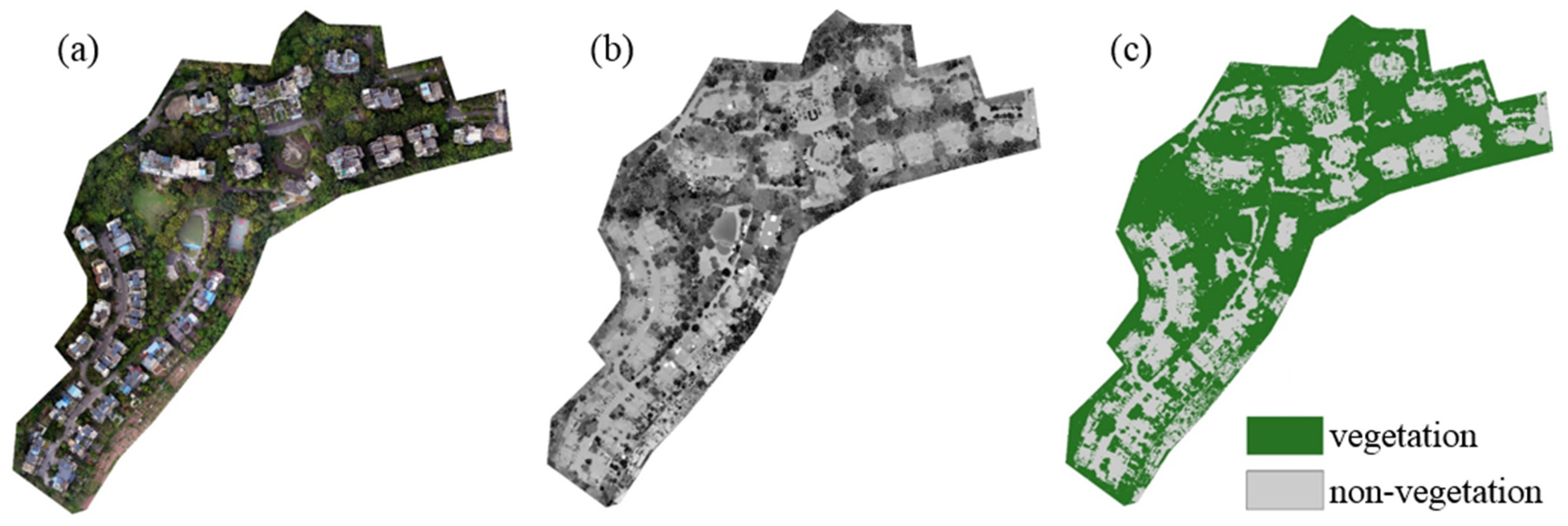
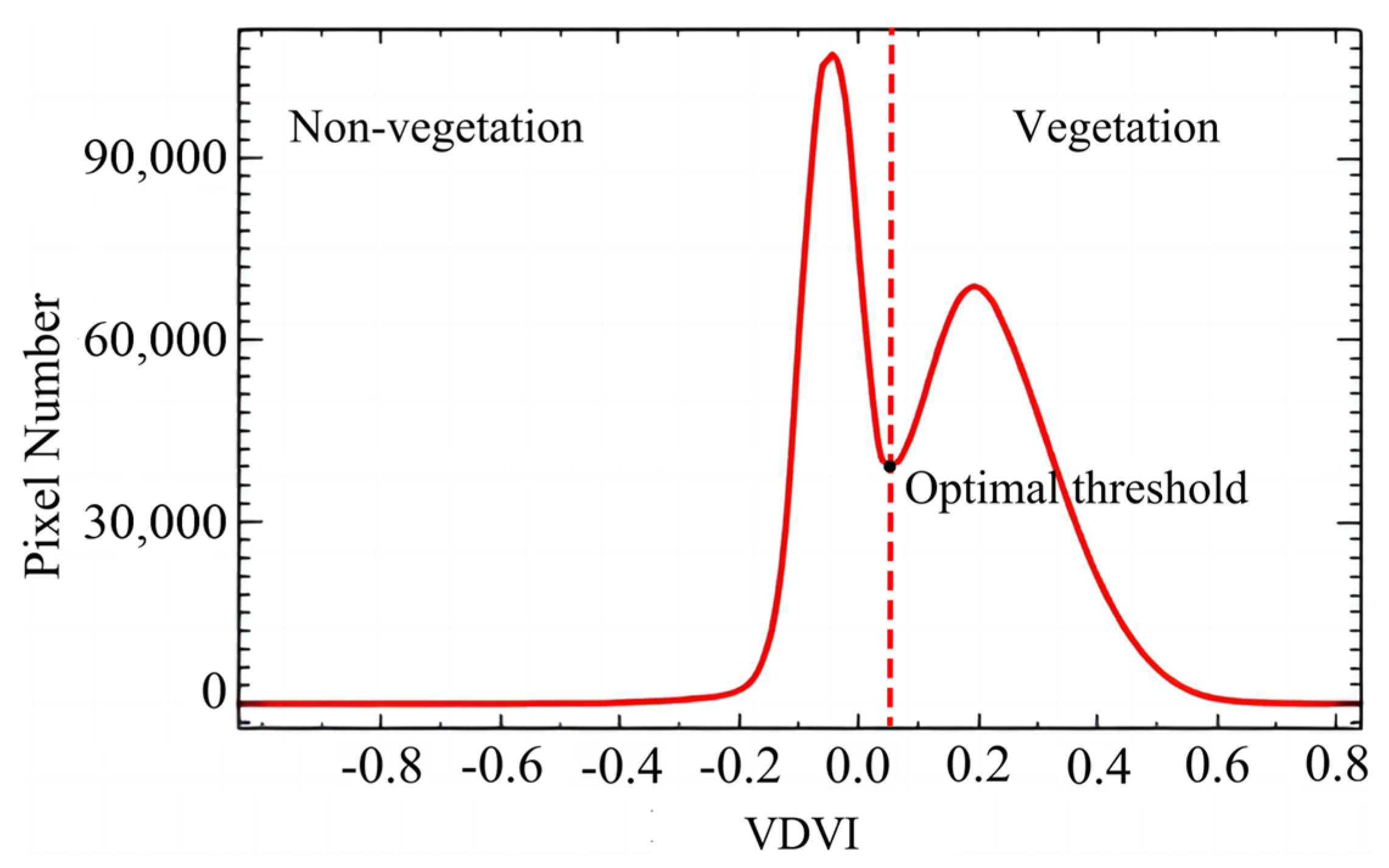
The vegetation extraction from the DOM of the residential community mainly involves two steps: calculating VDVI to quantify vegetation abundance and distinguishing vegetation from non-vegetation by setting a VDVI threshold. The determination of an appropriate threshold is crucial for vegetation extraction [36]. Compared to other vegetation indices, VDVI has a more pronounced bimodal characteristic [29], which can be used to determine the threshold, as proposed by Liang [37]. In the bimodal distribution of calculated VDVI values, one peak represents vegetation and the other represents the background. The VDVI value at the lowest point of the valley between the two peaks is determined as the optimal threshold to distinguish between vegetation and non-vegetation.

3.2.3. Metrics for Green Space Extraction Accuracy

The accuracy of vegetation extraction in the residential community is assessed using the standard confusion matrix for evaluating image classification accuracy, which mainly includes three metrics: kappa coefficient, UA (user accuracy), and PA (producer accuracy). The calculation formula for kappa coefficient based on the confusion matrix is as follows:

$$\begin{array}{c}Kappa={\displaystyle \frac{P_o-P_e}{1-P_e}}\end{array}$$

(2)

where $P_o$ represents the overall classification accuracy, which is the proportion of correctly classified samples in each class to the total number of samples; $P_e$ is the expected consistency rate calculated based on the confusion matrix, which is the sum of the products of the actual and predicted sample numbers for each class divided by the square of the total sample number.

The calculation formulas of UA and PA are as follows:

$$\begin{array}{c}UA={\displaystyle \frac{TP}{TP+FN}}\end{array}$$

(3)

$$\begin{array}{c}PA={\displaystyle \frac{TP}{TP+FP}}\end{array}$$

(4)

where TP (True Positive) is the number of samples correctly classified, FN (False Negative) is the number of samples incorrectly classified as that class, and FP (False Positive) is the number of samples in a class unclassified as that class.

3.3. Household Counting

The household number is one of the two types of prerequisite information for calculating the average green space per household in a residential community. The most convenient method is to directly inquire with the property management unit or conduct on-site investigations, but due to factors such as privacy protection or access control, it is usually difficult to realize. Remote sensing technology, especially high-resolution images captured by drones, provides an alternative solution for obtaining the number of households. Usually, the exposed building components of each household, such as roofs, balconies, windows, etc., are used to count them. For low-rise buildings, it is relatively easier to obtain the number of households, which is directly determined according to the inverted V-shaped roofs. For high-rise buildings, the number of households can only be counted from the facade images through automatic recognition of featured building components. Since a household usually has only one exposed balcony in the target community, the YOLACT instance segmentation model is used to detect and count the balconies of high-rise buildings to achieve the household number.

3.3.1. YOLACT Model

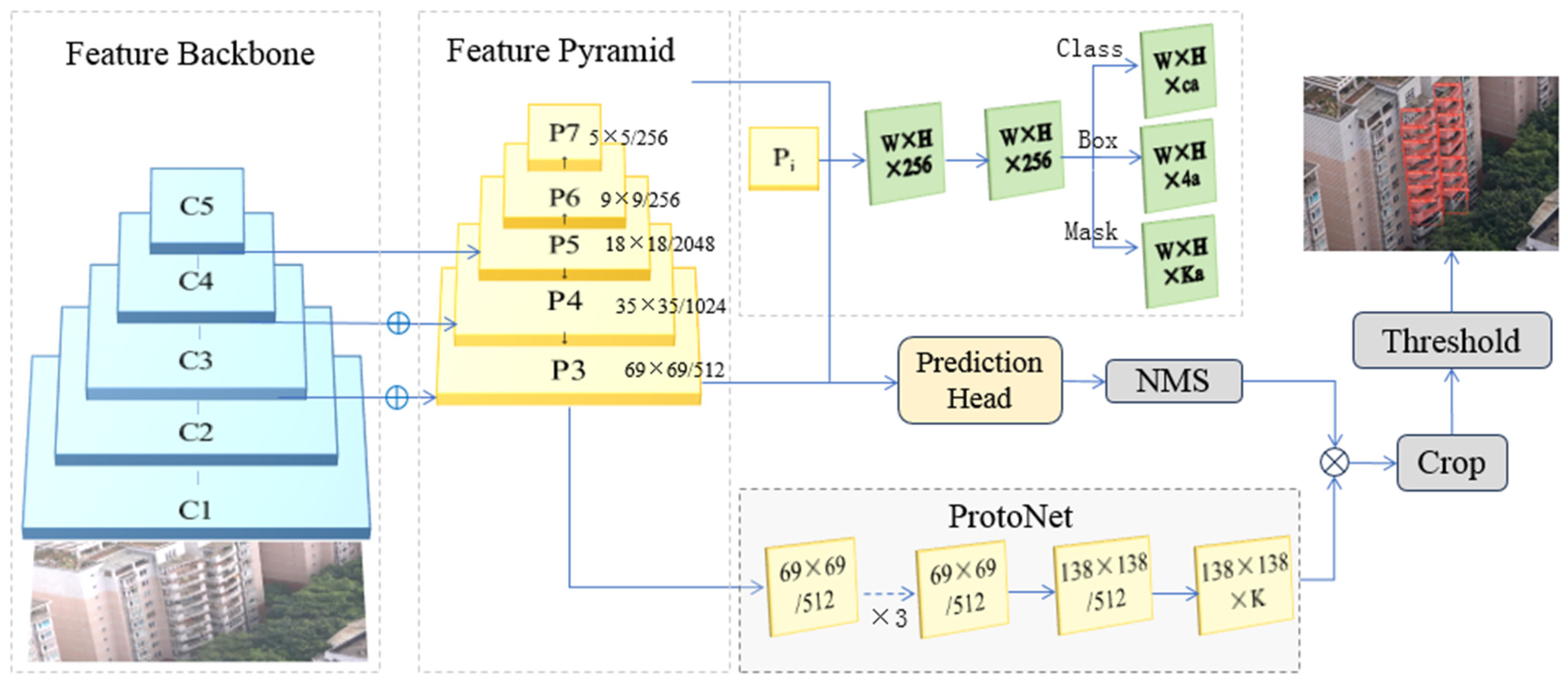
As indicated in Figure 2, the major components of the YOLACT network architecture include Feature Backbone, FPN (Feature Pyramid Net), ProtoNet (Prototype Mask Branch), and Prediction Head Branch [35]. The ProtoNet generates the prototype masks, while the prediction head branch creates the mask coefficient for predicting each instance. The two branches execute in parallel, and, finally, the prototype mask and mask coefficient are linearly combined to generate the instance mask. The YOLACT model usually uses the ResNet series as the backbone network to extract image features. In this study, the feature map generated by ResNet50 [38] is inputted into the FPN [39] to enhance the capability of multi-scale feature expressions, providing rich information for subsequent processing. In the two parallel subtasks, the prediction head branch is responsible for predicting the class and position of the target building component (balcony in this study) and outputting the class probability, bounding box coordinates, and mask coefficient of each bounding box; the ProtoNet adopts a fully convolutional network structure to generate prototype masks with the same resolution as the input images. Finally, by linearly combining the predicted mask coefficients with the corresponding prototype masks, instance masks are created to achieve instance segmentation of balconies. The major parameters of YOLACT, including batch size, training epochs, initial learning rate, etc., will be determined based on specific software and hardware configurations and model training efficiency.

3.3.2. Dataset Construction

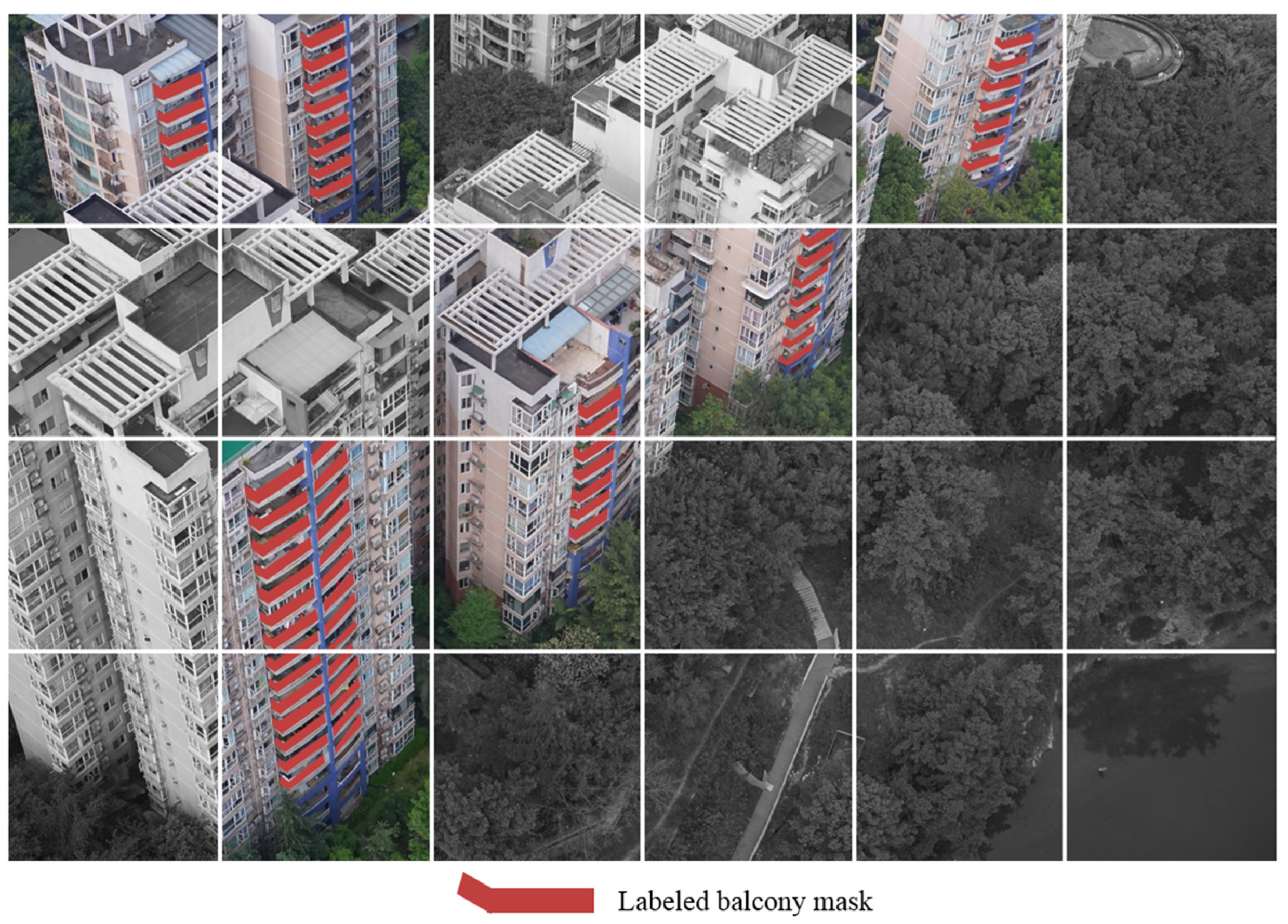
The clear images that contain facades of high-rise buildings are selected to form the initial dataset. The pixel size of the captured images is 6000 × 4000, but the size of a single balcony generally accounts for approximately 1% of an image. Additionally, the facade images typically have a complex environmental background. Hence, large images can lead to difficulties in instance segmentation and even memory overflow, while the resolution reduction through resampling will result in poor segmentation performance. To solve this problem, after the balcony masks in the image are manually labeled using the labelme tool [40], each original image including masks is partitioned into 24 non-overlapping blocks with a pixel size of 1000 × 1000. As seen in Figure 3, only the eight image blocks containing labeled balcony masks will be taken as initial datasets.

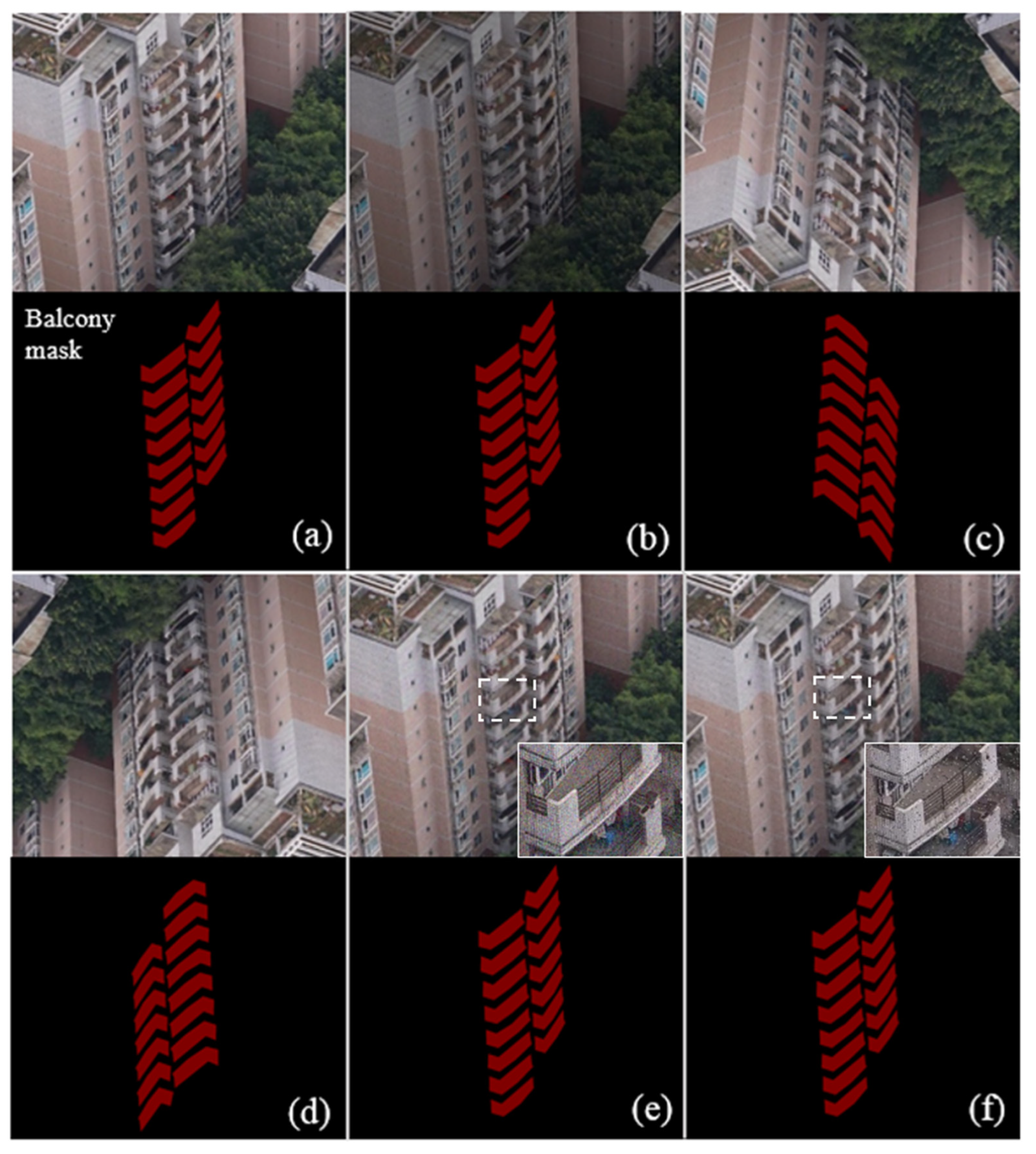
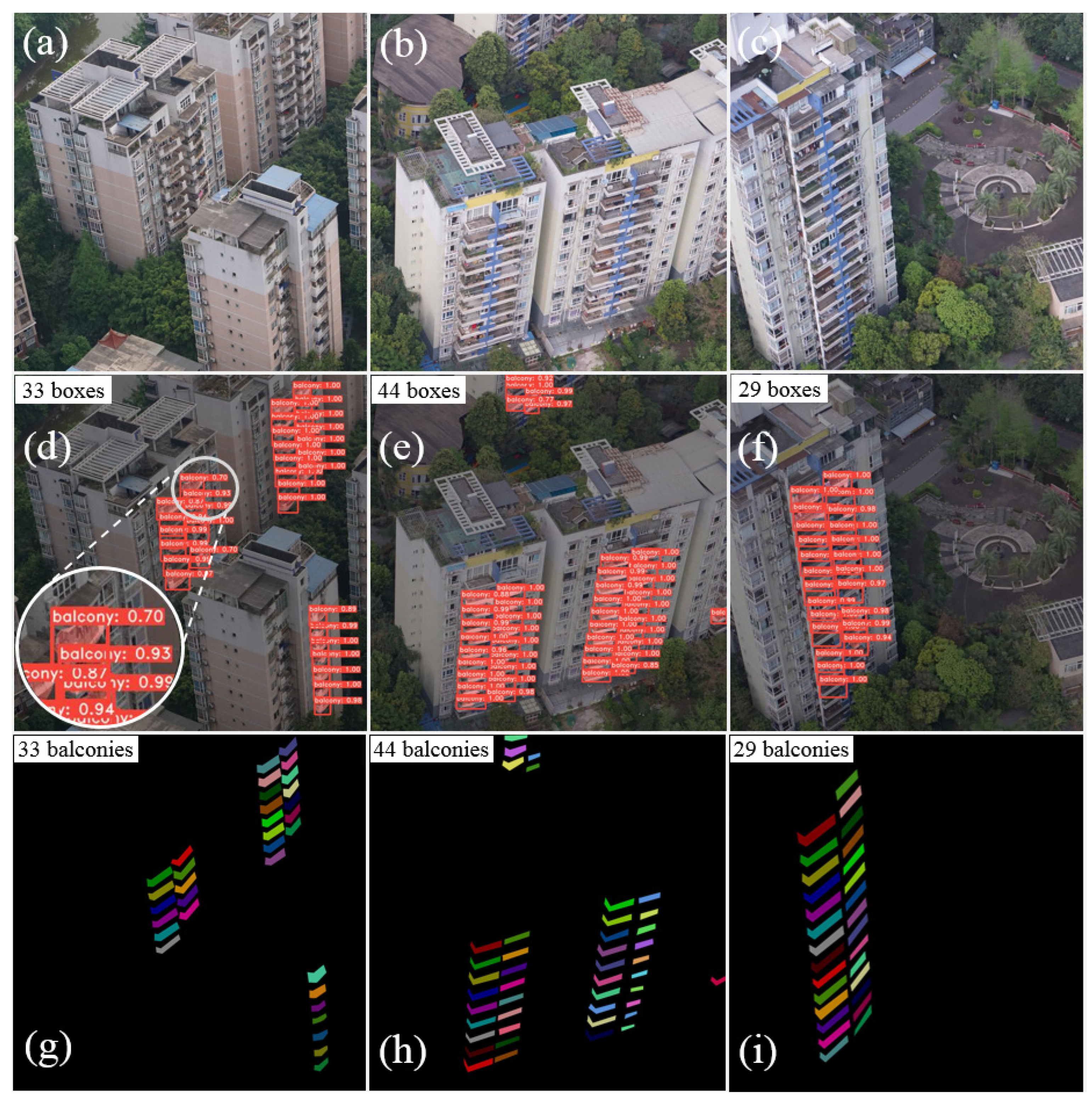
Data augmentation can largely increase the diversity of samples. When augmented data are used to train the model, they can significantly improve the performance of the model, enhance its robustness, and enrich the extracted features. The types of data augmentation mainly include color perturbation, geometric transformation, and noise addition. The facade image block of an example high building and its corresponding balcony masks are shown in Figure 4a, which will be used to illustrate various data augmentation types. Color perturbation refers to adjusting the brightness, saturation, and contrast of an image to simulate its states in various environments. As seen in Figure 4b, the brightness of the original image block is decreased. Geometric transformation refers to simulating the states at different positions and angles through rotation, flipping, and cropping. For example, the pairs of image blocks and balcony masks in Figure 4c,d are for vertical flipping and horizontal 180° rotation, respectively. Noise addition refers to adding various noises to an image to simulate poor imaging qualities in real scenarios. Figure 4e,f are the resulting image pairs added with Gaussian noise and random noise, respectively. All of the sample image pairs including original and augmented image blocks and annotated balcony masks are divided into a training set and a validation set in a ratio of 9:1.

3.3.3. Metrics for Balcony Recognition Accuracy

In this study, there is only one class of balcony involved, and the accuracy of balcony instance segmentation is evaluated using two key metrics: average precision (AP) and average recall (AR). The calculation formulas of AP and AR are as follows:

$$\begin{array}{c}AP={\sum }_{k=1}^{n}P\left(k\right)·∆P\left(k\right)\end{array}$$

(5)

$$\begin{array}{c}AR={\sum }_{k=1}^{n}R\left(k\right)·∆R\left(k\right)\end{array}$$

(6)

where $n$ is the total number of confidence thresholds; $P\left(k\right)$ is the precision at the k-th confidence threshold; $∆P\left(k\right)$ is the change in precision between the k-th and the k+1th confidence thresholds; $R\left(k\right)$ is the recall rate at the k-th confidence threshold; $∆R\left(k\right)$ is the change in recall rate between the k-th and the k+1th confidence thresholds.

For example, mAP₇₅ (m represents the number of class) denotes the average precision with an Intersection over Union (IoU) threshold of 0.75; mAP_all represents the average precision with an IoU threshold range of 0.5–0.95 and a step size of 0.05. IoU is defined as the overlap degree between the predicted box and the real box, that is, the overlap degree between the predicted balcony mask and the real balcony mask, which is used to measure the matching effect between the detected objects and the real ones. The calculation formula for IoU is as follows:

$$\begin{array}{c}IoU={\displaystyle \frac{A\cap B}{A\cup B}}\end{array}$$

(7)

where A represents the predicted box area measured in pixels; B is the actual box area measured in pixels.

4. Results

4.1. Extracted Green Space

After aerial triangulation and clipping, the resulting DOM of the study site (Figure 5a) was actually a large RGB image with a spatial resolution of 0.07 m and a coordination system of WGS84/UTM 48N. To extract the green space of the residential community, the VDVI of the entire community (Figure 5b) was calculated using Equation (1) based on the DOM, and we then generated a bimodal histogram (Figure 6) to determine the optimal threshold of VDVI as 0.055. The vegetation and non-vegetation classification results of the residential community are shown in Figure 5c. It should be noted that the pixels with VDVI values equal to the threshold were classified as vegetation.

As indicated in Figure 5c, the boundary between vegetation and non-vegetation regions is relatively clear. The vegetation accounted for 59.7% of the entire residential community, covering an area of approximately 0.051 km². This indicated that the overall green resources of the residential community were relatively abundant, and a high green space ratio could provide residents with sufficient green space. The vegetation in the high-rise building zone accounted for 70.8% of the total vegetation, while that in the low-rise building zone accounted for 29.2% of the total vegetation. The proportion of non-vegetation was 40.3% of the entire residential community, with an area of approximately 0.034 km². Among them, non-vegetation in the high-rise building zone accounted for 57.7% of the total non-vegetation, and that in the low-rise building zone was for 42.3% of the total non-vegetation.

4.2. Acquired Household Number

In this study, the CPU and GPU configurations for YOLACT model training and segmentation were Intel(R) Core (TM) i7-12700F 2.10 GHz and NVIDIA GeForce GTX 1650 4G, respectively. The software tools were Windows10, PyTorch version 1.2.1, and CUDA version 10.1.

In dataset construction, one or more of the data augmentation types were randomly used, and, finally, a total of 712 sample images and labeled masks were obtained. Then they were divided into a training set of 641 pairs and a validation set of 71 pairs. The feature extraction backbone network adopted the pretrained weights from ResNet-50 [41], and the training process employed a stochastic gradient descent (SGD) optimizer with a batch size of 2 and 200 training epochs. The initial learning rate was set to 2 × 10⁻³ [35]. Some of the convolutional layers in the pretrained model were frozen, resulting in higher initial performance. This not only saved training time but also improved the convergence effect of the model.

To achieve household numbers of all high-rise buildings in the residential community, the trained YOLACT model was applied to segment their facade images. Three typical facade images and recognized balconies are shown in Figure 7. Figure 7a–c show the original facade images of high buildings, Figure 7d–f show the bounding boxes of detected balconies, and Figure 7g–i show the segmented balcony instances. As illustrated in Figure 7d, the YOLACT model not only accurately located the balconies within the detection boxes but also generated a matching balcony mask for each detection box and labeled the probability of recognizing it as a balcony next to the detection box. In most cases, the model could accurately detect the position of the balcony and generate an instance mask that was consistent with the manually labeled one. As a result, it was determined that there were 702 households in the high-rise building zone. According to the inverted V-shaped roof, 50 households were identified in the low-rise building zone. Therefore, the total number of households in the residential community was counted to 752.

4.3. Average Green Space per Household

Based on the results from Section 4.1 and Section 4.2, the overall average green space per household in the residential community was calculated to be approximately 67.82 m². The average green space per household in the high-rise building zone was approximately 51.28 m², and that in the low-rise building zone was approximately 300 m².

According to Section 4.1, the green space area of the high-rise building zone was 0.036 km², and that of the low-rise zone was 0.015 km². Based on the areas of high-rise and low-rise building zones in Section 2.1, their green space ratios were calculated to be 65.5% and 50%, respectively. Based on the above results, the high-rise building zone indicated a certain advantage in terms of green space area and green space ratio. This was clearly contradictory to the design goals and actual feelings of green space resources and qualities in high-rise and low-rise building zones. In contrast, the average green space per household in the low-rise building zone was significantly higher than that in the high-rise building zone (300 m² vs. 51.28 m²), with a proportion of approximately 6:1. This result revealed a significant difference in the allocation of green space resources between the two zones, indicating that the traditional green space ratio index had obvious limitations in assessing the green space qualities of residential communities with large floor differences, while the household green space index could more accurately reflect the actual green space occupation in high- and low-rise building zones.

In future urban greening planning, the layout of green spaces in high-rise building zones should be further optimized, and the household green space should be raised to improve the living quality of local residents. Meanwhile, when evaluating the qualities of green spaces in residential communities, the average green space per household can be taken as an overall indicator, especially for the evaluation of residential communities with high-rise buildings.

4.4. Accuracy Assessment

4.4.1. Vegetation Extraction Accuracy

In this study, due to the difficulty in obtaining the true area of vegetation in the residential community, we used the average (Figure 8b) of multiple SVM-based classification results as the true value to assess the accuracy of vegetation extraction based on VDVI (Figure 8a). The classification accuracies of VDVI are shown in

Table 1. Classification accuracies of VDVI referring to the SVM-based classification result.

Classified data (VDVI)		Reference Data (SVM)
		Non-Vegetation/m2	Vegetation/m2	Total/m2	User Accuracy/%
	Non-vegetation/m2	27,451.93	2490.05	29,941.98	91.68
	Vegetation/m2	4356.91	50,701.10	55,058.02	92.09
	Total/m2	31,808.85	53,191.15	85,000
	Producer accuracy/%	86.30	95.32

. The overall classification accuracy of vegetation and non-vegetation reached 91.94%. The vegetation had a user accuracy of 92.09%, a producer accuracy of 95.32%, and a kappa coefficient of 0.89. These results indicated that the VDVI was very suitable for rapidly extracting green space from the DOM product of drone-acquired RGB images. Compared with supervised classification methods that require a large number of samples, the classification threshold of VDVI was relatively easier to determine, and the vegetation extraction accuracies were highly consistent.

4.4.2. Balcony Recognition Accuracy

The accuracy of the trained YOLACT model for balcony segmentation from facade images of high-rise buildings was assessed against the validation set. The AP and AR values of bounding boxes and instance masks under various IoU thresholds and maximum detection numbers are listed in

Table 2. The accuracies of YOLACT model for balcony segmentation.

Metric	IoU	MaxDets	Box	Mask
AP	0.5:0.95	100	0.844	0.311
AP	0.5	100	0.987	0.631
AP	0.75	100	0.977	0.683
AR	0.5:0.95	1	0.09	0.036
AR	0.5:0.95	10	0.751	0.282
AR	0.5:0.95	100	0.877	0.429

. As a whole, YOLACT demonstrated high detection accuracy. In most cases, the model could accurately identify the locations of balconies and generate masks in the detection boxes. Specifically, the accuracies of the detection boxes were much higher than those of the instance masks. The bounding boxes only displayed the locations of the balconies, while the masks provided the pixel-level shape information of balconies. In this study, accurate bounding boxes could satisfy the requirements for balcony positioning and recognition. At different IoU thresholds, the AP of the detection box reached 0.987 for boxAP₅₀ and 0.977 for boxAP₇₅, respectively. This indicated that the YOLACT model performed well at high confidence levels but poor at low confidence levels. The AR increased with the increment in the maximum detection number, indicating that the model could recognize more objects when allowing for more detections. It fully demonstrated the strong capability of YOLACT to accurately extract building components such as a balcony in complex scenes.

5. Discussion

5.1. Comparison of VDVI with Other Vegetation Indices

Using the appropriate vegetation index is the foundation for accurately extracting green space in the residential community. Therefore, several other RGB vegetation indices, including CIVE, EXGR, EXG, NGBDI, and NGRDI, were selected to compare with VDVI. Their calculation formulas are listed in

Table 3. The formulas of RGB vegetation indices.

Vegetation Index	Formula
CIVE	$\begin{array}{c}0.441{\rho }_{red}-0.881{\rho }_{green}+{0.386\rho }_{blue}+18.78745\end{array}$
EXGR	$\begin{array}{c}{3\rho }_{green}+2.4{\rho }_{red}-{\rho }_{blue}\end{array}$
EXG	$\begin{array}{c}{2\rho }_{green}-{\rho }_{red}-{\rho }_{blue}\end{array}$
NGBDI	$\begin{array}{c}{(\rho }_{green}-{\rho }_{blue})/({\rho }_{green}+{\rho }_{blue})\end{array}$
NGRDI	$\begin{array}{c}{(\rho }_{green}-{\rho }_{blue})/({\rho }_{green}+{\rho }_{blue})\end{array}$

Note: ρ_red, ρ_green, ρ_blue are the gray scale values of the red, green, and blue bands, respectively.

.

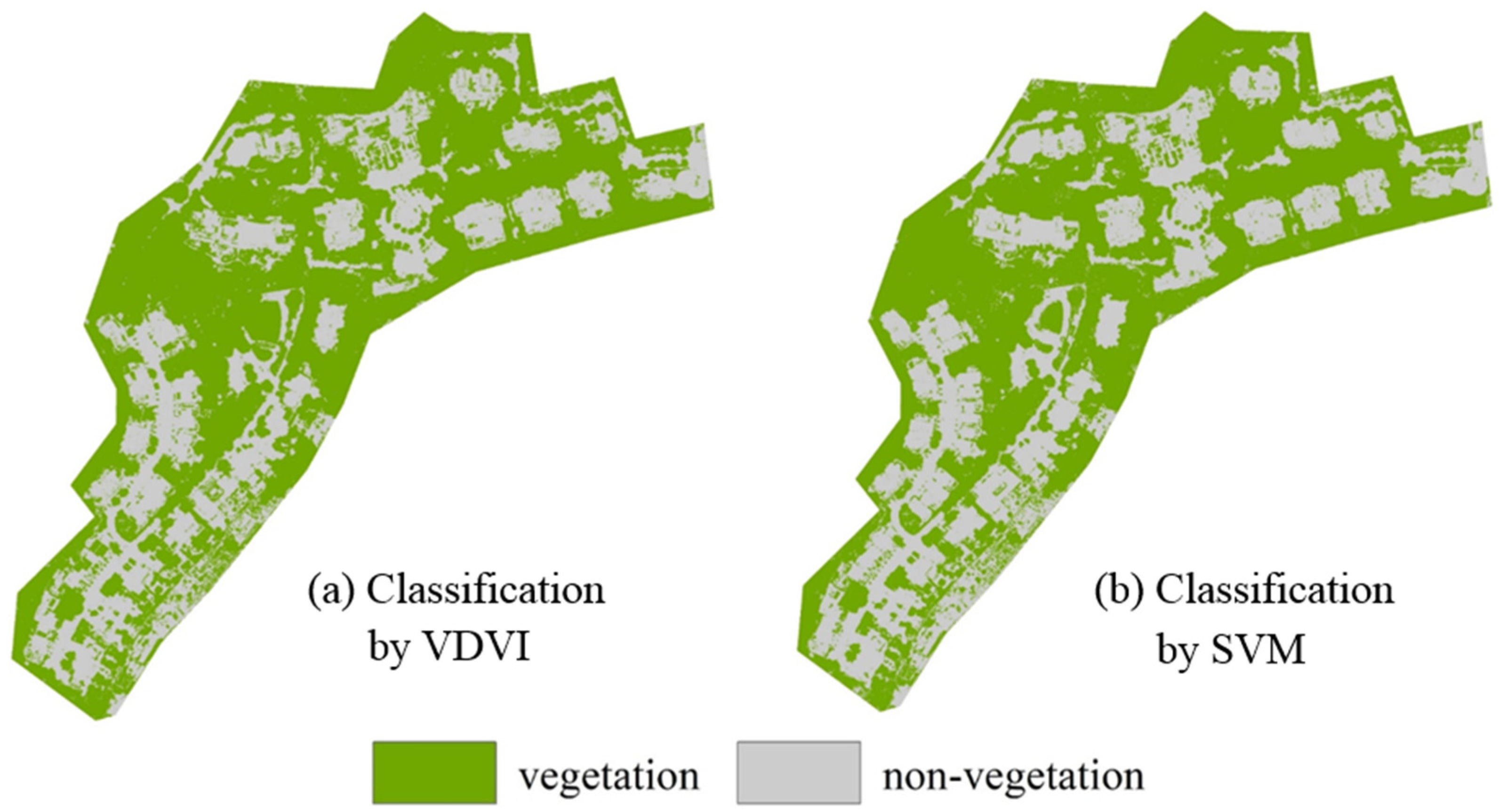
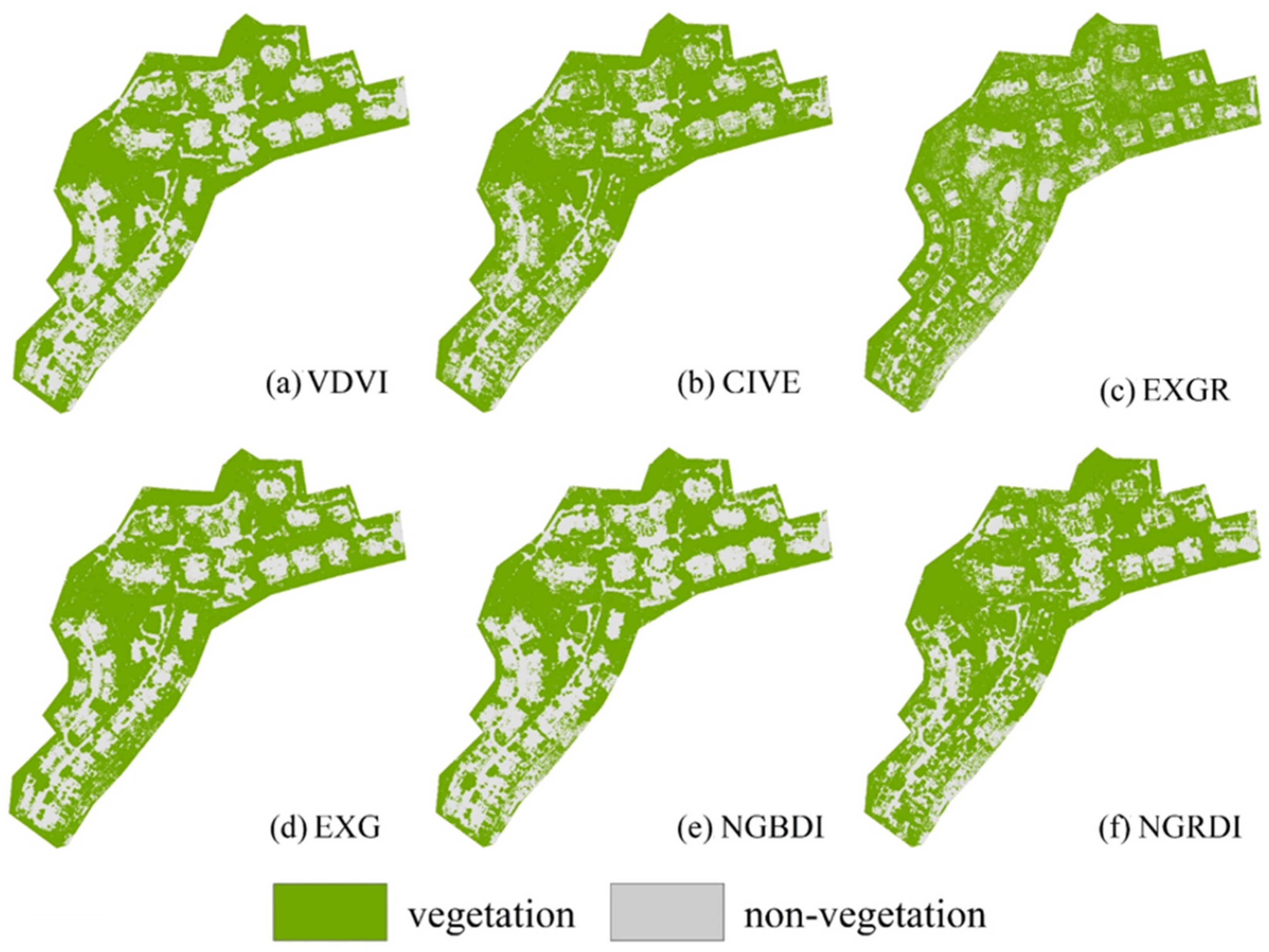
Classification maps of vegetation and non-vegetation based on various vegetation indices are shown in Figure 9, and their thresholds and classification accuracies are listed in

Table 4. The thresholds and classification accuracies of various RGB vegetation indices.

Vegetation Index	Threshold	Correct Rate%			Kappa Coefficient/%
		Vegetation	Non-Vegetation	Overall Accuracy
VDVI	0.055	92.09	91.68	91.94	88.92
CIVE	18.744	98.40	73.63	89.67	85.88
EXGR	0.615	83.28	55.34	73.43	57.78
EXG	0.074	92.58	89.15	91.37	88.10
NGBDI	0.035	94.83	82.86	90.62	87.09
NGRDI	0.039	93.06	73.01	85.99	80.13

. The classification results of VDVI, CIVE, EXG, and NGBDI (Figure 9a,b,d,e) were much better, with clear green space edges and building outlines. In contrast, those of EXGR and NGRDI (Figure 9c,f) had relatively blurred edges and could not distinguish vegetation and non-vegetation well. As seen in Table 4, the overall classification accuracies of all vegetation indices exceeded 85%, except for EXGR with 73.43%. Among them, VDVI performed the best, with the highest overall accuracy of 91.94%, kappa coefficient of 88.92%, and the user accuracies of both vegetation and non-vegetation exceeding 90%.

5.2. Comparison of YOLACT with Mask R-CNN

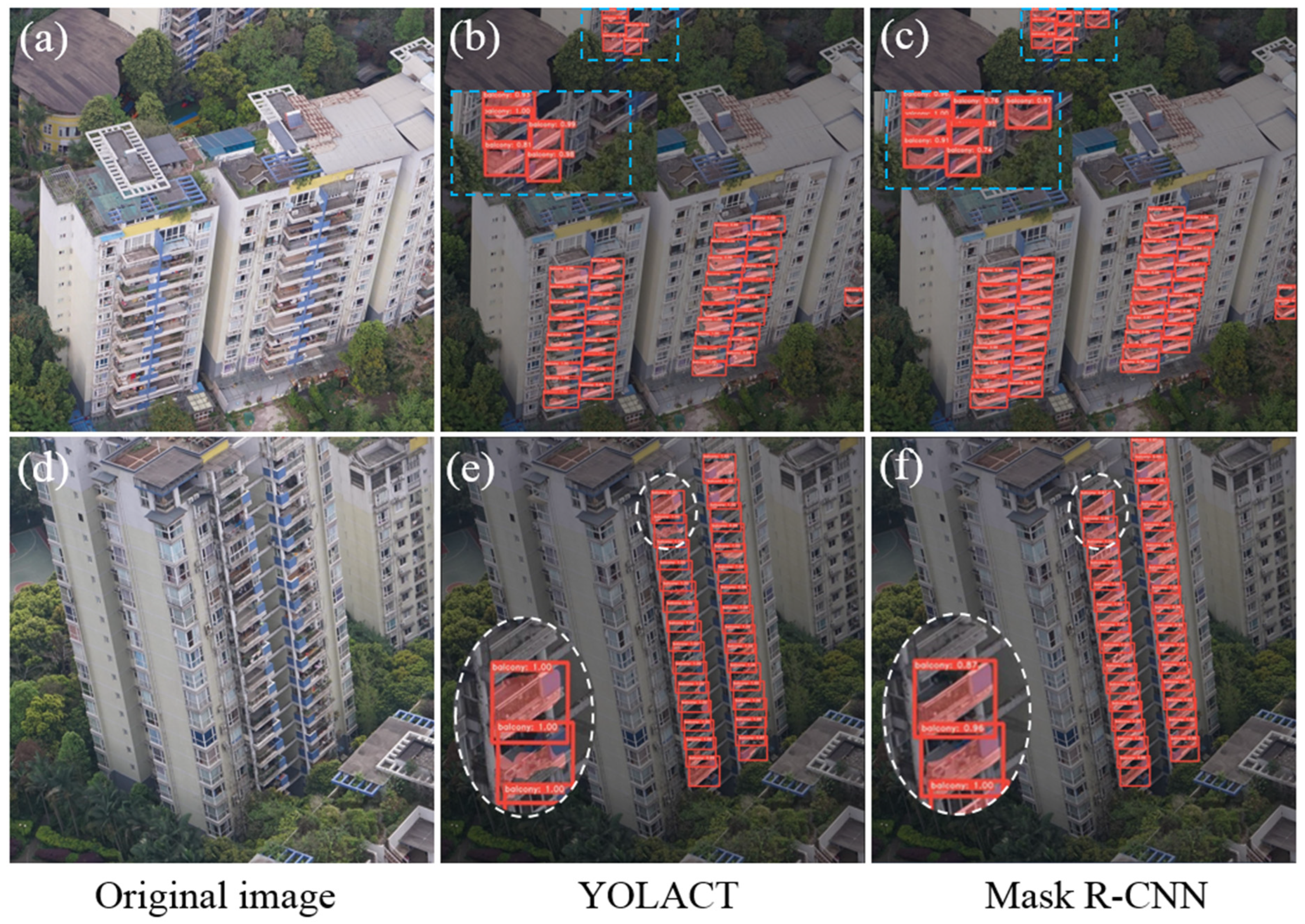
To further verify the effectiveness in extracting balconies from the facade images of high-rise buildings, the YOLACT model was compared with the Mask R-CNN model [34], which is commonly used in instance segmentation. The test balcony detection and segmentation results of YOLACT and Mask R-CNN are illustrated in Figure 10, while a detailed comparison of the two models on metrics including time consumption, AP and AR is given in

Table 5. Balcony detection and segmentation performances of YOLACT and Mask R-CNN.

Model	Instance	Time/ms	APall/%	AP50/%	AP75/%	ARall/%
YOLACT	box	65.67	84.4	98.7	97.7	87.7
	mask		31.1	63.1	68.3	42.9
Mask R-CNN	box	267.21	84.7	98.2	97.0	88.7
	mask		74.1	94.3	91.2	78.4

.

As shown in Figure 10, the two models exhibited high consistency in detecting the position and quantity of bounding boxes of balconies, but the recognition performance of YOLACT was slightly inferior in the partially exposed balconies at the edges of the images. As seen in the cyan dashed rectangles in Figure 10b,c, the numbers of balconies recognized by YOLACT and Mask R-CNN were five and seven, respectively. Additionally, Mask R-CNN was more accurate in balcony shape segmentation, while YOLACT had relatively poor performance in this regard. As indicated in the white dashed ellipses in Figure 10e,f, the balcony mask shapes in the detection boxes segmented by Mask R-CNN had a high degree of consistency with manually annotated ones, while those segmented by YOLACT differed considerably. Their sizes varied to varying degrees, and the edges were serrated.

As listed in Table 5, the two models exhibited high consistency in boxAP and boxAR, both performing well in the recognition of balcony boxes. Both of the boxAP_all exceeded 84%, while their boxAP₅₀ and boxAP₇₅ were both above 98% and 97%, respectively. In terms of boxAR_all, the performances were equally good, both exceeding 87%. In contrast, the maskAP values of YOLACT and Mask R-CNN differed significantly. The maskAP of YOLACT ranged from 30% to 70%, while that of Mask R-CNN was from 70% to 95%. Moreover, the maskAR_all value of YOLACT was only 42.9%, much less than 78.4% of Mask R-CNN.

Although YOLACT was inferior in balcony instance mask segmentation, it exhibited a significant advantage in bounding box detection speed. The detection time of Mask R-CNN was almost four-times that of YOLACT (267.21 ms vs. 65.67 ms). When selecting a suitable instance segmentation model, we needed to comprehensively consider the segmentation accuracy and detection speed of various models according to the study objective. In terms of balcony location and quantity detection, YOLACT indicated no obvious difference from Mask R-CNN, while demonstrating a significant real-time advantage. As the focus of this study was to determine the number of households by detecting balconies, it commonly had a lower accuracy requirement for the balcony instance mask. The balcony mask shapes were only used as auxiliary information for balcony instance judgment. Therefore, YOLACT could soundly achieve our study objective with a higher detection speed.

5.3. Limitations and Future Work

In this study, we conducted preliminarily explored obtaining household green space in a composite residential community solely relying on drone oblique photography. Although the current technical solutions achieved the expected result, there were still some limitations.

First of all, the determination of the household number of high buildings by recognizing balconies from the facade images was based on the premise that there was a one-to-one correspondence between households and balconies in the residential community. However, in more general scenarios, some high buildings in certain communities frequently have more than one balcony per household, and, in this case, the household quantity needs to be converted based on specific corresponding relationships. On the other hand, the balcony size is relatively small compared to the entire facade image, making it difficult to recognize. In this study, a block partition scheme was used to tackle this issue. In the future, to achieve more accurate segmentation of balconies, multi-scale feature fusion can be used to enrich the detailed features of the target region. In the low-rise building zone, the building type was villa, and the household number was directly determined by visually interpreting the inverted V-shaped roofs. In subsequent research, the YOLACT model can also be used to automatically recognize and count the household number in the low-rise building zone.

Secondly, although the household number was determined from a 3D perspective (facade images of high-rise building), the green space extraction was still limited to the 2D orthorectified perspective (DOM). Due to its inability to express the quantitative differences in vegetation with different heights, it may lead to deviations in the actual measurement of vegetation greenness. In subsequent work, the DSM generated from drone oblique images can be used to obtain the 3D geometric shapes of trees, shrubs, and grasslands and further achieve estimation of the volume and greenery of vegetation at different heights. In addition, there is still a lot of information to be explored in building facade images, such as the windows inside the building, which are important channels for residents to indirectly access green spaces. The number and size of household windows can also greatly affect the residents’ experience of green spaces.

Thirdly, we elucidated the differences in accessibility to green space for the residents in high-rise and low-rise zones based on the average green space per household. It was actually a static analysis without considering the mobility of the residents. Due to the connectivity between the high-rise and low-rise zones, residents from different zones could access public green spaces located in both zones. On the other hand, the willingness of residents to visit green spaces is inversely proportional to distance, and nearby green spaces generally have the highest probability of being visited. Therefore, the static analysis of the difference in household green space in high-rise and low-rise zones in a residential community still has certain significance. In future research, it may be considered to incorporate distance-based green space accessibility into the analysis of differences in household green spaces within residential communities. It is expected to further improve the precision of green space analysis in residential communities and achieve more precise evaluation of their green space qualities.

6. Conclusions

RGS is one of the major indicators for evaluating the quality of a residential community. With the emergence of high-rise buildings in modern cities, traditional green space indicators such as the green space ratio cannot truly reflect the green space resources enjoyed by household residents in residential communities. In contrast, average green space per household considers the differences in building floors between various residential communities or different zones within a residential community. However, there were frequently difficulties in acquiring the specific green space area and household number through ground surveys or consulting with property management units. In this study, we solely employed drone oblique photography to separately obtain the green space area and household number in a composite residential community, thereby achieving average green space per household and analyzing its zonal differences. The principal conclusions reached are as follows:

• The VDVI was able to efficiently extract the green space area from drone-acquired oblique RGB images by determining the optimal threshold value for separating vegetation and non-vegetation using a bimodal histogram.
• The YOLACT instance segmentation model was able to rapidly detect bounding boxes of balconies from the facade images of high-rise buildings to accurately count the household numbers.
• Although the green space ratio was relatively low in the low-rise building zone, the average green space per household was significantly higher than that in the high-rise building zone, with a ratio of approximately 6:1.
• Among six RGB vegetation indices, VDVI performed the best in green space extraction, with the highest overall accuracy of 91.94% and a kappa coefficient of 88.92%.
• Compared with the Mask R-CNN model, YOLACT was inferior in segmenting balcony shapes but exhibited a significant advantage in detection speed. The time consumed by YOLACT is only a quarter of that of Mask R-CNN.

Nevertheless, there were still some limitations in achieving average green space per household using drone oblique photography in this study, including singular correspondence between household and balcony, 2D-level green space extraction, static analysis of different accessibility to green space in low- and high-rise building zones. In the future, this study can be further advanced by addressing the aforementioned limitations. For example, one-to-many correspondence between household and building components shall be taken into consideration; the volume and greenery of vegetation at different heights shall be estimated using the local DSM and DEM; the mobility of the residents in the high-rise and low-rise zones shall be counted to dynamically analyze the green space accessibility.

In summary, the feasibility and effectiveness of using drone oblique photography alone to estimate the average green area per household in modern residential communities were demonstrated through this study. Drone oblique photography can greatly reduce ground investigations, overcome access restrictions, and decrease the difficulties in obtaining green space area and household number. The average green area per household is a very promising indicator to more accurately reflect the green space quality of residential communities with high-rise buildings. It is expected to promote more rational planning and design of green spaces in modern residential communities, improve the fairness of green space resource allocation, and ultimately enhance the overall living quality of local residents.