Adaptive Array Shape Estimation and High-Resolution Sensing for AUV-Towed Linear Array Sonar During Turns

Abstract

The deformation of the array shape during the turning process of an autonomous underwater vehicle (AUV)-towed line array sonar can significantly degrade its remote sensing performance. In this paper, a method for circular arc array modeling and dynamic deformation estimation is proposed. By treating the array shape as a hyperparameter, an adaptive central angle (shape) marginal likelihood maximization (ASMLM) algorithm is derived to jointly estimate the array shape and the directions of arrival (DOAs) of sources. The high-resolution ASMLM algorithm is used to improve the DOA estimation performance, effectively suppress left–right ambiguity and significantly reduce computational complexity, making it suitable for AUV platforms with limited computational resources. Experimental results from sea trials in the South China Sea are used to validate the superior performance of the proposed method over existing methods.

1. Introduction

Autonomous underwater vehicles (AUVs) are increasingly utilized for various underwater tasks due to their high mobility, stealth, and cost-effectiveness [1,2,3,4,5,6]. To meet the growing demands of marine exploration, remote sensing, surveillance, and anti-submarine warfare [3,7,8,9], AUVs are often equipped with sonar systems [9,10]. Early AUV sonar systems typically used conformal arrays mounted on the AUV hull, but the aperture of these systems is limited by the physical size of the AUV, restricting their ability to perform low-frequency [11], remote sensing. To address this limitation, towed arrays have been adopted for AUVs [1,11,12,13,14], providing larger apertures and thus improving detection performance [11,15].

However, several challenges are faced by the AUV-towed linear array, particularly due to the limited towing force and energy capacity of the AUV. These arrays are typically thinner and shorter than those towed by ships, making them more susceptible to shape deformations. During turns or encounters with ocean currents [16,17], significant bending of the towed linear array occurs [16,17,18,19,20,21], causing it to deviate from its expected straight-line shape. This bending introduces array shape mismatch, severely degrading the performance of the AUV’s sensing system. Additionally, the directivity of the towed linear array exhibits conical symmetry, resulting in left–right ambiguity [22] in the source DOA estimation.

The towed linear array shape estimation methods are generally divided into non-acoustic and acoustic methods. Traditionally, the shape of a towed linear array can be estimated using non-acoustic sensors [4,16,17,18,23], but this increases installation complexity and cost, making such methods unsuitable for the AUV-towed linear array. Alternatively, the array shape can be estimated based on received acoustic data [24,25]. 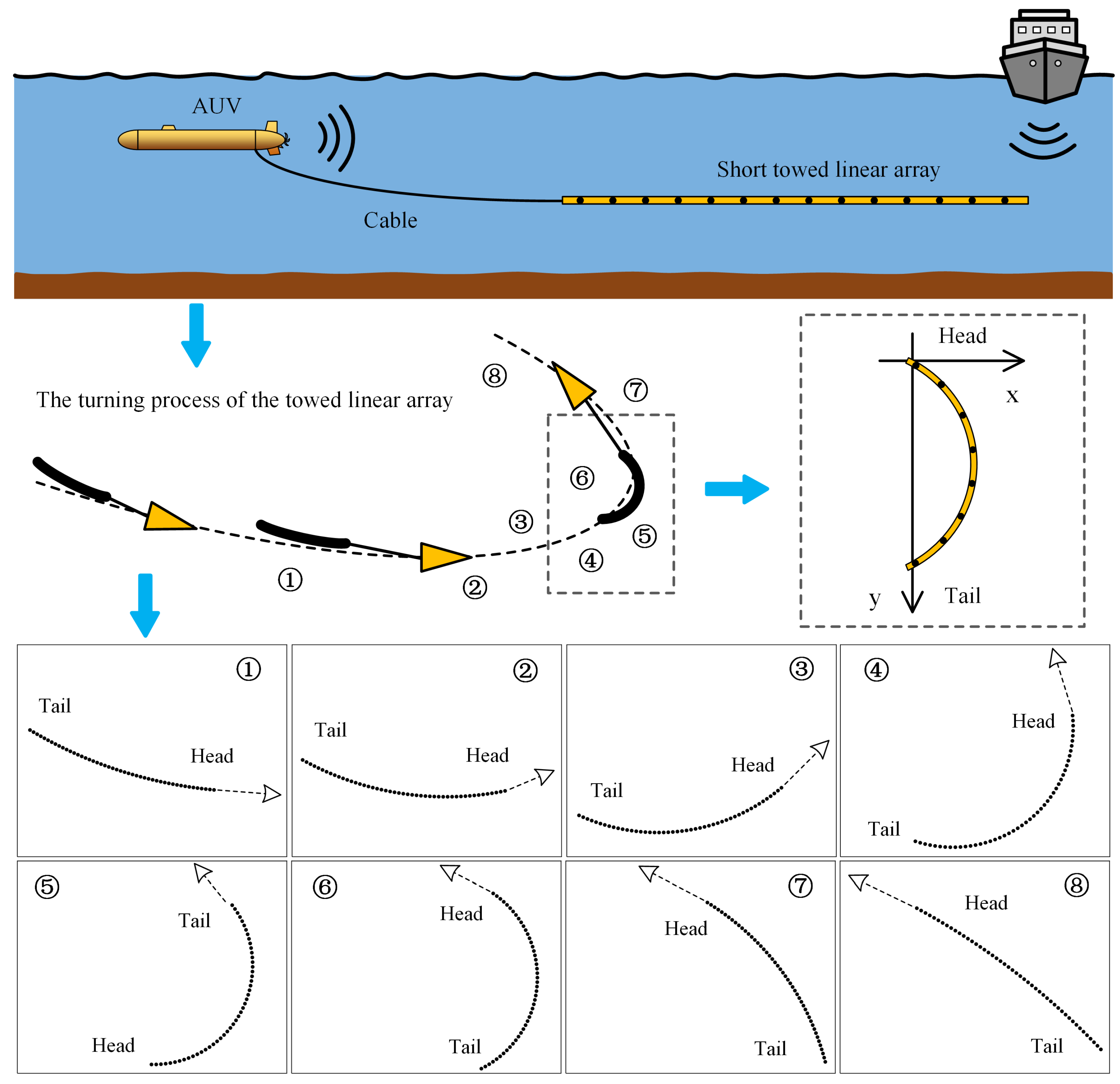In general, the shape of a towed linear array is modeled as either a parabola curve [18,20,21] or a circular arc [26], with the parabolic model being suitable for slow turns [18]. The schematic of the array shape variation in the AUV-towed linear array during the turning process is shown in Figure 1. The actual array shape is complex, making it challenging to accurately describe using simple mathematical models. To simplify this complexity, a circular arc model is adopted in this study to approximate the array overall shape, facilitating subsequent optimization and problem-solving. Although modeling a circular arc is simple, accurately estimating the dynamic changes in the arc shape during the turn is a challenging task.

In addition to modeling challenges, limited computational resources are faced by AUVs, necessitating the development of low-complexity algorithms capable of achieving high-resolution sensing. Conventional beamforming (CBF) offers fast computation but low resolution [27], while algorithms such as estimation of signal parameters via rotational invariance technique (ESPRIT) and multiple signal classification (MUSIC) provide high resolution but struggle with performance in scenarios with insufficient snapshots or low signal-to-noise ratios (SNR) [28]. Sparse Bayesian Learning (SBL) [29,30,31] methods provide a solution by offering high-resolution capabilities even under challenging conditions, such as the adaptive bow SBL (ABSBL) method [18]. However, high computational complexity is typically associated with these methods [32], making them impractical for AUV platforms.

To address these challenges, a circular arc modeling approach for the AUV-towed linear array is proposed. Importantly, the model is conceptually simple, the curvature of the array overall shape is represented by a single parameter, the central angle, which avoids complex parameter coupling and reduces the computational burden. By treating the central angle as an unknown parameter to be estimated, a more precise array manifold matrix can be obtained, thereby improving the estimation performance and mitigating the effects of shape deformation.

In addition, a low-complexity sparse Bayesian learning method tailored for AUV-towed linear arrays is developed. This method addresses the computational limitations of AUV platforms while maintaining high-resolution sensing capabilities. Leveraging sparse signal reconstruction and gradient-based optimization, the proposed approach jointly estimates array shape and source directions of arrival (DOAs). Additionally, by considering array shape deformation, left–right ambiguity is resolved without the need for extra sensors or hardware.

The main contributions of this paper are as follows:

(1) Novel Array Shape Modeling and Estimation: A circular arc model for a towed linear array during turning is proposed. By introducing the central angle as a hyperparameter in the marginal likelihood function, the dynamically changing array shape is estimated, which leads to an accurate array manifold matrix, mitigating array shape mismatch and improving the DOA estimation performance.

(2) Low-Complexity Sparse Bayesian Learning: Considering the computational resource constraints of AUV platforms, a fast sparse Bayesian learning algorithm is derived. The array shape and source directions of arrival are efficiently estimated by this algorithm, enabling high-resolution remote sensing.

(3) Resolution of Left–Right Ambiguity: By incorporating the deformation of the array shape into the estimation process, the left–right ambiguity is effectively resolved when the towed linear array is bent, using only the acoustic data received by the array. The accuracy of the source DOA estimation is enhanced without the need for additional hardware or sensor support.

The remainder of the paper is organized as follows. The circular arc modeling method for the towed linear arrays and direction of arrival estimation are presented in Section 2. The proposed algorithm, termed adaptive central angle (shape) marginal likelihood maximization (ASMLM) method, which jointly addresses the direction of arrival estimation of the source and the array shape estimation, is introduced in Section 3. The computational efficiency, array shape estimation, spatial spectrum estimation performance, and left–right ambiguity suppression effects of the proposed algorithms are discussed in Section 4 through simulation analysis. The effectiveness of the algorithms is validated using experimental data from the South China Sea in Section 5. The conclusions are provided in Section 6.

2. Array Shape Modeling and Direction of Arrival Estimation Problem

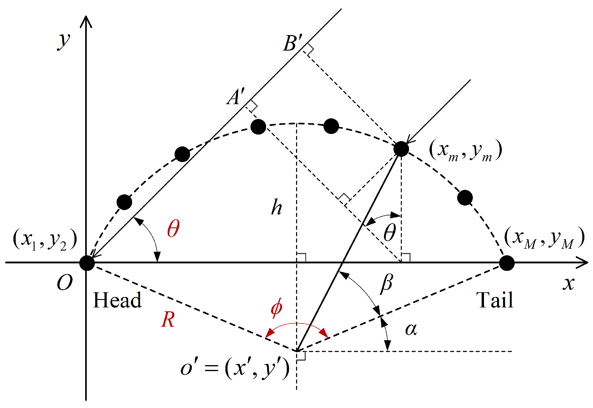
Consider a towed linear array with M elements, as shown in Figure 2. In the established coordinate system, the position of the array head (element 1) is at the origin O, with coordinates $(x_1,y_1)$. The x-axis is defined as the direction from the array head to the tail. The array shape is modeled as a circular arc, with the central angle $\varphi$ in radians given by

$$\varphi ={\displaystyle \frac{D}{R}},$$

(1)

where D is the arc length, which also serves as the aperture of a straight array, and R is the radius of the arc. The height of the arc chord is

$$h=R\left(1-cos\left({\displaystyle \frac{\varphi }{2}}\right)\right).$$

(2)

Assuming the shape of the towed linear array is a minor arc, i.e., $\varphi <\pi$, the coordinates of its arc center $o^{\prime }$ are $(x^{\prime },y^{\prime })$, given by

$$x^{\prime }=Rsin\left({\displaystyle \frac{\varphi }{2}}\right),y^{\prime }=-Rcos\left({\displaystyle \frac{\varphi }{2}}\right).$$

(3)

The coordinates of element m, denoted as $(x_m,y_m)$, where $m\in [1,\dots ,M]$, are expressed as

$$\begin{array}{cc}\hfill x_m& =x^{\prime }+Rcos(\alpha +\beta ),\hfill \\ \hfill y_m& =y^{\prime }+Rsin(\alpha +\beta ),\hfill \end{array}$$

(4)

where

$$\alpha ={\displaystyle \frac{\pi }{2}}-{\displaystyle \frac{\varphi }{2}},\beta =\varphi -{\displaystyle \frac{m-1}{M-1}}\varphi ={\displaystyle \frac{M-m}{M-1}}\varphi .$$

(5)

Substituting $\alpha$ and $\beta$ into $(\alpha +\beta )$ gives

$$\alpha +\beta ={\displaystyle \frac{\pi }{2}}-{\displaystyle \frac{\varphi }{2}}+{\displaystyle \frac{M-m}{M-1}}\varphi .$$

(6)

Substituting Equations (3) and (6) into Equation (4), and simplifying, the coordinates of element m are derived as

$$\begin{array}{cc}\hfill x_m& =Rsin\left({\displaystyle \frac{\varphi }{2}}\right)+Rsin\left({\displaystyle \frac{\varphi }{2}}-{\displaystyle \frac{M-m}{M-1}}\varphi \right),\hfill \\ \hfill y_m& =-Rcos\left({\displaystyle \frac{\varphi }{2}}\right)+Rcos\left({\displaystyle \frac{\varphi }{2}}-{\displaystyle \frac{M-m}{M-1}}\varphi \right).\hfill \end{array}$$

(7)

The source’s DOA $\theta$ is defined as the grazing angle relative to the x-axis. The measurement equation for the DOA estimation problem is given by

$$\mathbf{Y}=\mathbf{AS}+\mathbf{N},$$

(8)

where $\mathbf{Y}=[\mathbf{y}\left(1\right),\mathbf{y}\left(2\right),\dots ,\mathbf{y}\left(L\right)]\in {\mathbb{C}}^{M\times L}$, with L denoting the number of snapshots. The column vector $\mathbf{y}\left(l\right)={\left[y_1\left(l\right),y_2\left(l\right),\dots ,y_M\left(l\right)\right]}^{\mathrm{T}}\in {\mathbb{C}}^{M\times 1}$, for $l\in [1,\dots ,L]$. The array manifold matrix is $\mathbf{A}=\left[\mathbf{a}\left({\theta }_1\right),\mathbf{a}\left({\theta }_2\right),\dots ,\mathbf{a}\left({\theta }_N\right)\right]\in {\mathbb{C}}^{M\times N}$, where N is the number of grid points, and the column vector $\mathbf{a}\left({\theta }_n\right)={\left[{\mathbf{a}}_1\left({\theta }_n\right),\dots ,{\mathbf{a}}_M\left({\theta }_n\right)\right]}^{\mathrm{T}}\in {\mathbb{C}}^{M\times 1}$. The m-th element of $\mathbf{a}\left({\theta }_n\right)$ is ${\mathbf{a}}_m\left({\theta }_n\right)=exp\left(-j\omega {\tau }_m\right)$, where $n\in [1,\dots ,N]$, $\omega =2\pi f$, and f is the frequency. The time delay ${\tau }_m$ for element m relative to the reference element (element 1) is given by ${\tau }_m={\displaystyle \frac{O{B}^{\prime }}{c}}$, where c is the speed of sound. The sound path difference $O{B}^{\prime }$ between element m and element 1 is shown in Figure 2, where $O{B}^{\prime }=O{A}^{\prime }+A^{\prime }{B}^{\prime }$, with $O{A}^{\prime }=x_{m}cos{\theta }_n$ and $A^{\prime }{B}^{\prime }=y_{m}sin{\theta }_n$. Thus, we have

$${\tau }_m={\displaystyle \frac{x_{m}cos{\theta }_n+y_{m}sin{\theta }_n}{c}}.$$

(9)

The m-th element of $\mathbf{a}\left({\theta }_n\right)$ can be expressed as

$$\mathbf{a}\left({\theta }_n\right)=exp\left(-j{\displaystyle \frac{2\pi f}{c}}(x_{m}cos{\theta }_n+y_{m}sin{\theta }_n)\right).$$

(10)

Substituting Equations (1) and (7) into Equation (10), the m-th element of $\mathbf{a}\left({\theta }_n\right)$ can be expressed as

$$\begin{array}{cc}\hfill {\mathbf{a}}_m\left({\theta }_n\right)& =exp(-j{\displaystyle \frac{2\pi f}{c}}[\left(Rsin\left({\displaystyle \frac{\varphi }{2}}\right)+Rsin\left({\displaystyle \frac{\varphi }{2}}-{\displaystyle \frac{M-m}{M-1}}\varphi \right)\right)cos{\theta }_n\hfill \\ \hfill & +\left(-Rcos\left({\displaystyle \frac{\varphi }{2}}\right)+Rcos\left({\displaystyle \frac{\varphi }{2}}-{\displaystyle \frac{M-m}{M-1}}\varphi \right)\right)sin{\theta }_n\left]\right)\hfill \\ \hfill & =exp(-j{\displaystyle \frac{2\pi f}{c}}{\displaystyle \frac{D}{\varphi }}[\left(sin\left({\displaystyle \frac{\varphi }{2}}\right)+sin\left({\displaystyle \frac{\varphi }{2}}-{\displaystyle \frac{M-m}{M-1}}\varphi \right)\right)cos{\theta }_n\hfill \\ \hfill & +\left(-cos\left({\displaystyle \frac{\varphi }{2}}\right)+cos\left({\displaystyle \frac{\varphi }{2}}-{\displaystyle \frac{M-m}{M-1}}\varphi \right)\right)sin{\theta }_n\left]\right)\hfill \end{array}.$$

(11)

In Equation (8), the source matrix $\mathbf{S}=\left[\mathbf{s}\right(1),\mathbf{s}(2),\dots ,$$\mathbf{s}\left(L\right)]\in {\mathbb{C}}^{N\times L}$, where $\mathbf{s}\left(l\right)={[s_1\left(l\right),s_2\left(l\right),\dots ,s_N\left(l\right)]}^{\mathrm{T}}\in {\mathbb{C}}^{N\times 1}$. The noise matrix $\mathbf{N}=[\mathbf{n}\left(1\right),\mathbf{n}\left(2\right),\dots ,\mathbf{n}\left(L\right)]\in {\mathbb{C}}^{M\times L}$ contains the noise vectors, with each column vector $\mathbf{n}\left(l\right)={[n_1\left(l\right),n_2\left(l\right),\dots ,n_M\left(l\right)]}^{\mathrm{T}}\in {\mathbb{C}}^{M\times 1}$ representing white Gaussian noise for the l-th snapshot.

Assume that $K\ll N$ sources impinge on the M-element towed linear array. The received array data $\mathbf{Y}$ is known, and $\mathbf{S}$ is a row-sparse matrix, where only the rows corresponding to the K source directions are non-zero, while all other rows contain zero elements. Consequently, by identifying the non-zero rows $i\in {\mathcal{I}}_K$, the DOAs of the sources can be estimated. This transforms the DOA estimation problem into a sparse reconstruction problem for $\mathbf{S}$ based on Equation (8).

3. The Proposed Method

Since the arc length D of the towed linear array is fixed, the array shape can be uniquely determined by the central angle $\varphi$. Therefore, estimating $\varphi$ from the received data directly yields the array shape. As both the sources and the array shape are unknown, this constitutes a joint estimation problem.

In Equation (8), assuming the noise follows an independent zero-mean Gaussian distribution, the noise variance for the l-th snapshot is ${\sigma }_l^2$, such that $p\left(\mathbf{n}\left(l\right)\right)=\mathcal{N}(0,{\sigma }_l^2\mathbf{I})$. The likelihood function can then be expressed as [29,30,33]

$$p(\mathbf{Y}\mid \mathbf{S};\varphi ,{\sigma }^2)=\prod _{l=1}^L\mathcal{CN}(\mathbf{y}\left(l\right);\mathbf{A}\mathbf{s}\left(l\right),{\sigma }_l^2\mathbf{I}),$$

(12)

where $\mathcal{CN}(·)$ denotes the complex Gaussian distribution. Assuming $s_n\left(l\right)$ follows a Gaussian distribution with variance ${\gamma }_n$, the prior of the source signals is given by

$$p(\mathbf{S};\mathit{\gamma })=\prod _{l=1}^L\prod _{n=1}^{N}p(s_n\left(l\right);{\gamma }_n)=\prod _{l=1}^L\mathcal{CN}(\mathbf{s}\left(l\right);\mathbf{0},\mathbf{\Gamma }),$$

(13)

where $\mathit{\gamma }=[{\gamma }_1,\dots ,{\gamma }_N]$, each snapshot $\mathbf{s}\left(l\right)$ is a multivariate Gaussian with covariance matrix $\mathbf{\Gamma }=diag\left(\mathit{\gamma }\right)$. Within the Bayesian estimation framework, the posterior of the source signals $\mathbf{S}$ can be derived by combining the likelihood of the array observations $\mathbf{Y}$ with the prior of the source signals:

$$p(\mathbf{S}\mid \mathbf{Y};\mathit{\gamma },\varphi ,{\sigma }^2)={\displaystyle \frac{p(\mathbf{Y}\mid \mathbf{S};\varphi ,{\sigma }^2)p(\mathbf{S};\mathit{\gamma })}{p(\mathbf{Y};\mathit{\gamma },\varphi ,{\sigma }^2)}},$$

(14)

where $p(\mathbf{Y};\mathit{\gamma },\varphi ,{\sigma }^2)$ is the evidence. The posterior $p(\mathbf{S}\mid \mathbf{Y};\mathit{\gamma },\varphi ,{\sigma }^2)$ follows a complex Gaussian distribution with mean $\mathit{\mu }$ and covariance $\mathbf{\Sigma }$ [29,33,34]:

$$p(\mathbf{S}\mid \mathbf{Y};\mathit{\gamma },\varphi ,{\sigma }^2)=\mathcal{CN}(\mathit{\mu },\mathbf{\Sigma }),$$

(15)

where

$$\begin{array}{cc}\hfill & \mathbf{\Sigma }={\left({\mathbf{\Gamma }}^{-1}+{\sigma }^{-2}{\mathbf{A}}^{\mathrm{H}}\mathbf{A}\right)}^{-1},\hfill \\ \hfill & \mathit{\mu }={\sigma }^{-2}\mathbf{\Sigma }{\mathbf{A}}^{\mathrm{H}}\mathbf{Y}.\hfill \end{array}$$

(16)

The evidence is given by

$$p(\mathbf{Y};\mathit{\gamma },\varphi ,{\sigma }^2)={\int }_{-\infty }^{\infty }p(\mathbf{Y}\mid \mathbf{S};\varphi ,{\sigma }^2)p(\mathbf{S};\mathit{\gamma })d\mathbf{S}.$$

(17)

Taking the logarithm of Equation (17) yields [29,33]

$$\mathcal{F}(\mathit{\gamma },\varphi ,{\sigma }^2)=logp(\mathbf{Y};\mathit{\gamma },\varphi ,{\sigma }^2)\propto -log\left|\mathbf{P}\right|-tr\left({\mathbf{Y}}^{\mathrm{H}}{\mathbf{P}}^{-1}\mathbf{Y}\right),$$

(18)

where $\mathbf{P}={\sigma }^2\mathbf{I}+\mathbf{A}\mathbf{\Gamma }{\mathbf{A}}^{\mathrm{H}}$. The hyperparameters $\mathit{\gamma }$, $\varphi$, and ${\sigma }^2$ are estimated by maximizing the log marginal likelihood function:

$$\left(\widehat{\mathit{\gamma }},\widehat{\varphi },{\widehat{\sigma }}^2\right)=\underset{\mathit{\gamma }\ge 0,0<\varphi <\pi ,{\sigma }^2>0}{argmax}\mathcal{F}\left(\mathit{\gamma },\varphi ,{\sigma }^2\right).$$

(19)

Simultaneous updates of the three hyperparameters $\mathit{\gamma }$, $\varphi$, and ${\sigma }^2$ do not always lead to an optimal solution and can significantly increase computational complexity. This is because updating the central angle $\varphi$ is to estimate the array shape, that is, to modify the array manifold matrix $\mathbf{A}$, while updating $\mathit{\gamma }$ and ${\sigma }^2$ aims to obtain the optimal DOA estimation result under the current array manifold matrix $\mathbf{A}$.

Therefore, our update strategy begins with initializing $\varphi$. Once $\mathit{\gamma }$ and ${\sigma }^2$ are updated to a suboptimal DOA estimate under the current array shape, $\varphi$ is updated based on the current estimates of $\mathit{\gamma }$ and ${\sigma }^2$. These steps are repeated until the convergence condition is met or the maximum number of iterations is reached.

3.1. Direction of Arrival Estimation

The sparse reconstruction of the source signal is achieved by solving the closed-form solution of the signal variance in spatial domain $\mathit{\gamma }$, which enables the fast estimation of the angle of arrival. By fixing the array shape hyperparameter $\varphi$ and maximizing the log marginal likelihood function, the partial derivative of $\mathcal{F}(\mathit{\gamma },\varphi ,{\sigma }^2)$ with respect to ${\mathit{\gamma }}_n$ is

$${\displaystyle \frac{\partial \mathcal{F}(\mathit{\gamma },\varphi ,{\sigma }^2)}{\partial {\mathit{\gamma }}_n}}={∥{\mathbf{Y}}^{\mathrm{H}}{\mathbf{P}}^{-1}\mathbf{a}\left({\theta }_n\right)∥}_2^2-L\mathbf{a}{\left({\theta }_n\right)}^{\mathrm{H}}{\mathbf{P}}^{-1}\mathbf{a}\left({\theta }_n\right).$$

(20)

Setting Equation (20) equal to zero yields ${∥{\mathbf{Y}}^{\mathrm{H}}{\mathbf{P}}^{-1}\mathbf{a}\left({\theta }_n\right)∥}_2^2=L\mathbf{a}{\left({\theta }_n\right)}^{\mathrm{H}}{\mathbf{P}}^{-1}\mathbf{a}\left({\theta }_n\right)$. By multiplying both sides by ${\mathit{\gamma }}_n$, we obtain ${\mathit{\gamma }}_n{∥{\mathbf{Y}}^{\mathrm{H}}{\mathbf{P}}^{-1}\mathbf{a}\left({\theta }_n\right)∥}_2^2={\mathit{\gamma }}_{n}L\mathbf{a}{\left({\theta }_n\right)}^{\mathrm{H}}{\mathbf{P}}^{-1}\mathbf{a}\left({\theta }_n\right)$, which does not have a closed-form solution [30]. To improve computational efficiency, we rewrite the logarithmic marginal likelihood. The covariance matrix $\mathbf{P}$ in Equation (18) can be decomposed as [33,34]

$$\mathbf{P}={\sigma }^2\mathbf{I}+{\displaystyle \sum _{n\ne i}}\mathbf{a}\left({\theta }_n\right){\mathit{\gamma }}_n\mathbf{a}{\left({\theta }_n\right)}^{\mathrm{H}}+\mathbf{a}\left({\theta }_i\right){\mathit{\gamma }}_i\mathbf{a}{\left({\theta }_i\right)}^{\mathrm{H}}.$$

(21)

Defining $\mathbf{E}={\sigma }^2\mathbf{I}+{\displaystyle \sum _{n\ne i}}\mathbf{a}\left({\theta }_n\right){\mathit{\gamma }}_n\mathbf{a}{\left({\theta }_n\right)}^{\mathrm{H}}$, where $\mathbf{E}$ represents the component of $\mathbf{P}$ after removing the contribution from $\mathbf{a}\left({\theta }_i\right)$. Thus, Equation (21) can be expressed as $\mathbf{P}=\mathbf{E}+\mathbf{a}\left({\theta }_i\right){\mathit{\gamma }}_i\mathbf{a}{\left({\theta }_i\right)}^{\mathrm{H}}$. Substituting this into Equation (18), the marginal likelihood $\mathcal{F}(\mathit{\gamma },\varphi ,{\sigma }^2)$ can be rewritten as

$$\begin{array}{cc}\hfill \mathcal{F}(\mathit{\gamma },\varphi ,{\sigma }^2)& =-log\left|\mathbf{E}+\mathbf{a}\left({\theta }_i\right){\mathit{\gamma }}_i\mathbf{a}{\left({\theta }_i\right)}^{\mathrm{H}}\right|-{\mathbf{Y}}^{\mathrm{H}}{\left(\mathbf{E}+\mathbf{a}\left({\theta }_i\right){\mathit{\gamma }}_i\mathbf{a}{\left({\theta }_i\right)}^{\mathrm{H}}\right)}^{-1}\mathbf{Y}\hfill \\ \hfill & =-log\left|\mathbf{E}\right|-{\mathbf{Y}}^{\mathrm{H}}{\mathbf{E}}^{-1}\mathbf{Y}+log\left({\mathit{\gamma }}_i^{-1}\right)-log\left({\mathit{\gamma }}_i^{-1}+s_i\right)+{\displaystyle \frac{u_i^2}{{\mathit{\gamma }}_i^{-1}+s_i}}\hfill \\ \hfill & =\mathcal{E}({\mathit{\gamma }}_{n\ne i},\varphi ,{\sigma }^2)+\mathcal{C}({\mathit{\gamma }}_i,\varphi ,{\sigma }^2),\hfill \end{array}$$

(22)

where

$$\mathcal{C}({\mathit{\gamma }}_i,\varphi ,{\sigma }^2)=log\left({\mathit{\gamma }}_i^{-1}\right)-log\left({\mathit{\gamma }}_i^{-1}+s_i\right)+{\displaystyle \frac{u_i^2}{{\mathit{\gamma }}_i^{-1}+s_i}},$$

(23)

with

$$s_i=\mathbf{a}{\left({\theta }_i\right)}^{\mathrm{H}}{\mathbf{E}}^{-1}\mathbf{a}\left({\theta }_i\right),u_i=\mathbf{a}{\left({\theta }_i\right)}^{\mathrm{H}}{\mathbf{E}}^{-1}\mathbf{Y}.$$

(24)

The hyperparameter ${\mathit{\gamma }}_i$ is obtained by taking the partial derivative of Equation (18) as follows:

$${\displaystyle \frac{\partial \mathcal{F}(\mathit{\gamma },\varphi ,{\sigma }^2)}{\partial {\mathit{\gamma }}_i^{-1}}}={\displaystyle \frac{\partial \mathcal{C}({\mathit{\gamma }}_i,\varphi ,{\sigma }^2)}{\partial {\mathit{\gamma }}_i^{-1}}}={\displaystyle \frac{(s_i-u_i^2)+{\mathit{\gamma }}_i{s}_i^2}{{({\mathit{\gamma }}_i^{-1}+s_i)}^2}}.$$

(25)

Setting Equation (25) equal to zero yields the closed-form solution for ${\mathit{\gamma }}_i$:

$${\mathit{\gamma }}_i=\left(u_i^2-s_i\right)/\phantom{\left(u_i^2-s_i\right)s_i^2}{s}_i^2.$$

(26)

For computational convenience, $s_i$ and $u_i$ are expressed as:

$$s_i={\displaystyle \frac{S_i}{1-{\mathit{\gamma }}_i{S}_i}},u_i={\displaystyle \frac{U_i}{1-{\mathit{\gamma }}_i{S}_i}},$$

(27)

where

$$S_i=\mathbf{a}{\left({\theta }_i\right)}^{\mathrm{H}}{\mathbf{P}}^{-1}\mathbf{a}\left({\theta }_i\right),U_i=\mathbf{a}{\left({\theta }_i\right)}^{\mathrm{H}}{\mathbf{P}}^{-1}\mathbf{Y}.$$

(28)

Using the Woodbury matrix identity [33], we compute

$$S_i={\sigma }^{-2}\mathbf{a}{\left({\theta }_i\right)}^{\mathrm{H}}\mathbf{B}\mathbf{a}\left({\theta }_i\right),U_i={\sigma }^{-2}\mathbf{a}{\left({\theta }_i\right)}^{\mathrm{H}}\mathbf{B}\mathbf{Y},$$

(29)

where $\mathbf{B}=(\mathbf{I}-\mathbf{A}\mathbf{\Sigma }{\mathbf{A}}^{\mathrm{H}}{\sigma }^{-2})$. The hyperparameter ${\sigma }^2$ is coupled with ${\mathit{\gamma }}_n$. In practice, ${\sigma }^2$ is treated as a regularizer and fixed to ${\sigma }^2=\eta {\parallel \mathbf{Y}\parallel }_2^2$, reducing computational complexity [35], with $\eta$ adjusted based on different signal-to-noise ratios.

To improve computational efficiency, we calculate only $S_i$ and $U_i$, with $s_i$ and $u_i$ computed only when needed according to the formulas in Equation (27). When $i\notin {\mathcal{I}}_K$, we set ${\mathit{\gamma }}_i=0$, which leads to $s_i=S_i$ and $u_i=U_i$. Initializing ${\mathit{\gamma }}_n=0$, we have $\mathbf{P}={\sigma }^2\mathbf{I}+\mathbf{A}\mathbf{\Gamma }{\mathbf{A}}^{\mathrm{H}}={\sigma }^2\mathbf{I}$, and thus ${\mathbf{P}}^{-1}={\sigma }^{-2}\mathbf{I}$. From Equation (28), we can calculate

$$S_n={\sigma }^{-2}\mathbf{a}{\left({\theta }_n\right)}^{\mathrm{H}}\mathbf{a}\left({\theta }_n\right),U_n={\sigma }^{-2}\mathbf{a}{\left({\theta }_n\right)}^{\mathrm{H}}\mathbf{Y},$$

(30)

obtain all the ${\mathit{\gamma }}_n$ to be updated, namely

$${\tilde{\mathit{\gamma }}}_n=\left(u_i^2-s_i\right)/\phantom{\left(u_i^2-s_i\right)s_i^2}{s}_i^2=\left(U_n^2-S_n\right)/\phantom{\left(U_n^2-S_n\right)S_n^2}{S}_n^2.$$

(31)

Substituting ${\tilde{\mathit{\gamma }}}_n$ into Equation (23), we select the ${\mathit{\gamma }}_i$ that maximizes $\mathcal{C}({\mathit{\gamma }}_i,\varphi ,{\sigma }^2)$. Then, we compute ${\mathbf{\Sigma }}_{ii}={({\mathit{\gamma }}_i^{-1}+S_i)}^{-1}$, and ${\mu }_i={\mathbf{\Sigma }}_{ii}{U}_i$. The update formulas for $S_n$ and $U_n$ are as follows:

$${\tilde{S}}_n=S_n-{\mathbf{\Sigma }}_{ii}{\left({\sigma }^{-2}\mathbf{a}{\left({\theta }_n\right)}^{\mathrm{H}}{b}_i\right)}^2,{\tilde{U}}_n=U_n-{\mathit{\mu }}_i\left({\sigma }^{-2}\mathbf{a}{\left({\theta }_n\right)}^{\mathrm{H}}{b}_i\right),$$

(32)

where $b_i\triangleq \mathbf{B}\mathbf{a}\left({\theta }_i\right)$. When $n\ne i$, $s_n={\tilde{S}}_n$, $u_n={\tilde{U}}_n$. When $n=i$, $s_n={\tilde{S}}_n/(1-{\mathit{\gamma }}_i{\tilde{S}}_n)$, $u_n={\tilde{U}}_n/(1-{\mathit{\gamma }}_i{\tilde{S}}_n)$. We update ${\tilde{\mathit{\gamma }}}_n$ using Equation (26), calculate Equation (23), select the next ${\mathit{\gamma }}_i$ that maximizes the value of Equation (23), and check if the termination condition is met. If convergence is not achieved, we continue updating $\tilde{\mathbf{\Sigma }}$ and $\tilde{\mathit{\mu }}$, as described in [21,33], and update $S_n$ and $Q_n$ accordingly. Typically, the number of array elements M is smaller than the number of grid points N. In the SBL algorithm based on expectation maximization, the main steps involve estimating $\mathbf{\Sigma }$ and $\mathit{\mu }$ to compute ${\mathit{\gamma }}_i$, where the computational complexities of $\mathbf{\Sigma }$ and $\mathit{\mu }$ are $\mathcal{O}\left(N^3\right)$ and $\mathcal{O}\left(M{N}^2\right)$, respectively. the main steps of the proposed algorithm compute ${\mathit{\gamma }}_i$ by estimating $S_n$ and $Q_n$, with a complexity of $\mathcal{O}\left(M^{2}N\right)$.

3.2. Array Shape Estimation

The array shape is determined by the hyperparameter $\varphi$, which is estimated from the received data. With fixed hyperparameters $\mathit{\gamma }$ and ${\sigma }^2$, we maximize the expression in (18) to obtain

$$\widehat{\varphi }=\underset{0<\varphi <\pi }{argmax}\mathcal{F}\left(\mathit{\gamma },\varphi ,{\sigma }^2\right).$$

(33)

Take the partial derivative of $\varphi$ in Equation (18):

$${\displaystyle \frac{\partial \mathcal{F}(\mathit{\gamma },\varphi ,{\sigma }^2)}{\partial \varphi }}={\displaystyle \frac{\partial \left(-log\left|\mathbf{P}\right|-tr\left({\mathbf{Y}}^{\mathrm{H}}{\mathbf{P}}^{-1}\mathbf{Y}\right)\right)}{\partial \varphi }}.$$

(34)

Using the chain rule, we derive

$${\displaystyle \frac{\partial (-log|\mathbf{P}\left|\right)}{\partial \varphi }}={\displaystyle \frac{\partial (-tr(log\left|\mathbf{P}\right|\left)\right)}{\partial \varphi }}=-tr\left({\mathbf{P}}^{-1}{\displaystyle \frac{\partial \mathbf{P}}{\partial \varphi }}\right),$$

(35)

$${\displaystyle \frac{\partial \left(-tr\left({\mathbf{Y}}^{\mathrm{H}}{\mathbf{P}}^{-1}\mathbf{Y}\right)\right)}{\partial \varphi }}=-tr\left({\mathbf{Y}}^{\mathrm{H}}{\displaystyle \frac{\partial {\mathbf{P}}^{-1}}{\partial \varphi }}\mathbf{Y}\right)=tr\left({\mathbf{Y}}^{\mathrm{H}}{\mathbf{P}}^{-1}{\displaystyle \frac{\partial \mathbf{P}}{\partial \varphi }}{\mathbf{P}}^{-1}\mathbf{Y}\right)$$

(36)

In Equation (35) and Equation (36), let $\mathbf{H}={\displaystyle \frac{\partial \mathbf{P}}{\partial \varphi }}$. The partial derivative of $\mathcal{F}(\mathit{\gamma },\varphi ,{\sigma }^2)$ with respect to $\varphi$ can then be written as

$${\displaystyle \frac{\partial \mathcal{F}(\mathit{\gamma },\varphi ,{\sigma }^2)}{\partial \varphi }}=tr\left({\mathbf{P}}^{-1}\mathrm{H}\right)-tr\left({\mathbf{Y}}^{\mathrm{H}}{\mathbf{P}}^{-1}\mathrm{H}{\mathbf{P}}^{-1}\mathbf{Y}\right),$$

(37)

where

$$\mathbf{H}={\displaystyle \frac{\partial \mathbf{P}}{\partial \varphi }}={\displaystyle \frac{\partial \left({\sigma }^2\mathbf{I}+\mathbf{A}\mathbf{\Gamma }{\mathbf{A}}^{\mathrm{H}}\right)}{\partial \varphi }}={\displaystyle \frac{\partial \mathbf{A}}{\partial \varphi }}\mathbf{\Gamma }{\mathbf{A}}^{\mathrm{H}}+\mathbf{A}\mathbf{\Gamma }{\left({\displaystyle \frac{\partial \mathbf{A}}{\partial \varphi }}\right)}^{\mathrm{H}}.$$

(38)

To compute ${\displaystyle \frac{\partial \mathbf{A}}{\partial \varphi }}$, the partial derivative of the m-th element ${\mathbf{a}}_m\left({\theta }_n\right)$ of $\mathbf{a}\left({\theta }_n\right)$ in $\mathbf{A}$ is given by:

$${\displaystyle \frac{\partial \left({\mathbf{a}}_m\left({\theta }_n\right)\right)}{\partial \varphi }}={\mathbf{a}}_m\left({\theta }_n\right)\left(-j{\displaystyle \frac{2\pi f}{c}}\right)\left(-{\displaystyle \frac{D}{{\varphi }^2}}G+{\displaystyle \frac{D}{\varphi }}{\displaystyle \frac{\partial G}{\partial \varphi }}\right),$$

(39)

where

$$G=\left(sin\left({\displaystyle \frac{\varphi }{2}}\right)+sin\left({\displaystyle \frac{\varphi }{2}}-{\displaystyle \frac{M-m}{M-1}}\varphi \right)\right)cos{\theta }_n+\left(-cos\left({\displaystyle \frac{\varphi }{2}}\right)+cos\left({\displaystyle \frac{\varphi }{2}}-{\displaystyle \frac{M-m}{M-1}}\varphi \right)\right)sin{\theta }_n$$

(40)

$$\begin{array}{cc}\hfill {\displaystyle \frac{\partial G}{\partial \varphi }}& =\left({\displaystyle \frac{1}{2}}cos\left({\displaystyle \frac{\varphi }{2}}\right)+\left({\displaystyle \frac{1}{2}}-{\displaystyle \frac{M-m}{M-1}}\right)cos\left({\displaystyle \frac{\varphi }{2}}-{\displaystyle \frac{M-m}{M-1}}\varphi \right)\right)cos{\theta }_n\hfill \\ \hfill & +\left({\displaystyle \frac{1}{2}}sin\left({\displaystyle \frac{\varphi }{2}}\right)-\left({\displaystyle \frac{1}{2}}-{\displaystyle \frac{M-m}{M-1}}\right)sin\left({\displaystyle \frac{\pi }{2}}-{\displaystyle \frac{M-m}{M-1}}\varphi \right)\right)sin{\theta }_n\hfill \end{array}.$$

(41)

The central angle $\varphi$ is obtained by applying the gradient descent method, which allows for the estimation of the towed linear array shape.

The proposed algorithm is summarized in Algorithm 1. The main steps are as follows: (a) The central angle $\varphi$ and noise variance ${\sigma }^2$ are initialized. (b) The array manifold matrix $\mathbf{A}$ is computed, followed by the calculation of $S_n$, $U_n$, and ${\tilde{\mathit{\gamma }}}_n$; subsequently, ${\mathit{\gamma }}_i$ is computed, the covariance ${\mathbf{\Sigma }}_{ii}$ and the mean ${\mathit{\mu }}_i$ are updated, and ${\tilde{S}}_n$ and ${\tilde{U}}_n$ are computed. (c) $s_n$ and $u_n$ are computed, ${\tilde{\mathit{\gamma }}}_n$ is updated, the next ${\mathit{\gamma }}_i$ is calculated, and $\tilde{\mathbf{\Sigma }}$, $\tilde{\mathit{\mu }}$ are updated, with ${\tilde{S}}_n$ and ${\tilde{U}}_n$ being computed. (d) The central angle $\varphi$ is updated using the gradient descent method. (e) The estimated central angle $\varphi$ and the variance $\mathit{\gamma }$ are output.

Algorithm 1 ASMLM

Input:  $\mathbf{Y}$ 1: Initialization: $\varphi$, ${\sigma }^2$ 2: repeat 3:   Compute $\mathbf{A}$ using ${\mathbf{a}}_m\left({\theta }_n\right)$ from Equation (11) 4:   Initialize ${\mathit{\gamma }}_n=0$, compute $S_n$, $U_n$ using Equation (30), and ${\tilde{\mathit{\gamma }}}_n$ using Equation (31) 5:   Select ${\mathit{\gamma }}_i$ maximizing Equation (23), update ${\mathbf{\Sigma }}_{ii}$, ${\mathit{\mu }}_i$ using Equation (16) 6:   Compute ${\tilde{S}}_n$, ${\tilde{U}}_n$ using Equation (32) 7:   repeat 8:      Compute $s_n$ and $u_n$: If $n\ne i$, set $s_n={\tilde{S}}_n$ and $u_n={\tilde{U}}_n$; otherwise, set $s_n={\tilde{S}}_n/(1-{\mathit{\gamma }}_i{\tilde{S}}_n)$ and $u_n={\tilde{U}}_n/(1-{\mathit{\gamma }}_i{\tilde{S}}_n)$. Update ${\tilde{\mathit{\gamma }}}_n$ using Equation (26) 9:      Select the next ${\mathit{\gamma }}_i$ maximizing Equation (23) 10:    Compute ${\mathbf{\Sigma }}_{ii}$ and ${\mathit{\mu }}_i$, then compute ${\tilde{S}}_n$ and ${\tilde{U}}_n$ using Equation (32), update $\tilde{\mathbf{\Sigma }}$ and $\tilde{\mathit{\mu }}$ 11:  until No more ${\mathit{\gamma }}_i$ is selected 12:  Optimize $\varphi$ using gradient descent based on Equations (33)–(41) 13: until Convergence of $\varphi$ Output:  $\varphi$ and $\mathit{\gamma }$

Steps (b) and (c) are primarily aimed at obtaining the optimal estimate of $\mathit{\gamma }$ under the current central angle $\varphi$, while step (d) optimizes the central angle $\varphi$ under the current $\mathit{\gamma }$. The number of iterations can be set according to practical needs. For example, if the number of sources K is known, computing ${\gamma }_i$ requires K iterations. If K is unknown, the number of updates for ${\gamma }_i$ should satisfy the spatial sparsity assumption, i.e., $K\ll N$. The iteration for $\varphi$ stops when the maximum number of iterations is reached, or when the set convergence rate is reached.

The proposed method is designed to address the problem of array shape and remote source DOA estimation in AUV-based ocean remote sensing systems using towed linear array sonar. It enhances the capability of remote target localization. With array shape estimation and array signal processing as its core techniques, the method holds significant potential for applications in underwater target detection, ocean acoustic imaging, and environmental parameter estimation.

4. Simulations

A simulation analysis of the performance of the proposed ASMLM method during the steady turning process of a towed linear array is conducted in this section. The analysis focuses on the computational efficiency of the algorithm, the array shape estimation performance, the spatial spectrum estimation performance, and the effectiveness of left–right ambiguity suppression.

Consider a 48-element towed linear array with an element spacing of 0.417 $\mathrm{m}$, a total aperture of approximately 19.6 $\mathrm{m}$, and a sound speed of 1540 $\mathrm{m}$/$\mathrm{s}$. The bearing-time-records (BTRs) [22] of the two sound sources is shown in Figure 3a, where the energy of Source 1 is 0 $\mathrm{dB}$, and its azimuth is varied from 65° to approximately 121°. The energy of Source 2 is $-6$ $\mathrm{dB}$, and its azimuth is varied from approximately 108° to 167°.

A total of 120 Pings were sampled throughout the turning process. Between Ping 40 and Ping 80, the array shape closely resembled a circular arc. The variation in chord height during the turn, which is used to quantify the degree of bending, is illustrated in Figure 3b. For non-arc-shaped configurations, the chord height is defined as the maximum y-axis coordinate of the array elements. Based on the water-pulley model, the evolution of the array shape at different Pings is shown in Figure 4, visually demonstrating the dynamic deformation characteristics of the array during the turning maneuver.

The processed frequency range is from 500 $\mathrm{Hz}$ to 560 $\mathrm{Hz}$. White noise with a power of $-15$ $\mathrm{dB}$ is added, and the number of frequency domain snapshots per ping is 50. The initial central angle $\varphi$ is set to 0.2 radians and $\eta$ is set to 0.1. The grid interval is set to 1°. The BTRs estimation results obtained by different methods are shown in Figure 5. The CBF and MUSIC algorithms are applied based on the conventional linear array model. The ABSBL algorithm is implemented using a parabolic array model. For the linear array, the azimuth estimation range is limited to 0°–180°. However, due to the bending of the array, the azimuth estimation range can be extended to 0°–360°, allowing the left or right azimuth of the sound source to be distinguished.

From Ping 1 to Ping 20, the array bending is slight, and the results processed based on the linear array model still allow the two source signals to be distinguished. From Ping 20 to Ping 100, significant array bending is observed, and the resulting shape mismatch severely affects the estimation performance of the CBF and MUSIC algorithms. The azimuths of the two sources are not successfully estimated by either algorithm. From Ping 100 to Ping 120, although the bending gradually decreases, the estimation of Source 2 remains ineffective for both algorithms, as it is weak and located near the endfire direction. The state-of-the-art ABSBL method performs well in estimating the two source signals from Ping 1 to Ping 30. From Ping 30 to Ping 100, a large curvature is present in the simulated array shape, while a parabolic model is adopted by the ABSBL algorithm. The array shape mismatch prevents the accurate estimation of the azimuths of both sources. From Ping 100 to Ping 120, the ability to estimate the weak Source 2 decreases. In contrast, both sources are consistently estimated throughout the entire process by the ASMLM method.

Additionally, as shown in

Table 1. The average computation time per ping at each frequency point.

	CBF	MUSIC	ABSBL	ASMLM
Time (s)	0.0021	0.0126	6.0862	0.3965

, the average computation time per ping at each frequency point is measured as 0.0021 $\mathrm{s}$, 0.0126 $\mathrm{s}$, 6.0862 $\mathrm{s}$, and 0.3965 $\mathrm{s}$ for CBF, MUSIC, ABSBL, and ASMLM, respectively. Although faster computation speeds are achieved by CBF and MUSIC, their estimation performance deteriorates under array bending and left–right ambiguity cannot be suppressed. The ABSBL algorithm shows good estimation performance when the central angle of the curved shape is not large, but its computation time is slower. In comparison, the ASMLM algorithm is found to effectively balance computation speed and estimation performance.

The spatial spectrum estimation results at different Pings are shown in Figure 6. In Figure 6a, the results at Ping 2 are presented, where the degree of the array is small. The MUSIC algorithm is sensitive to array shape mismatch, and the estimated power of Source 2 differs significantly from the true power. In contrast, the other methods accurately estimate both the azimuth and power of the two sources, among which ABSBL and ASMLM both show the best left–right ambiguity suppression. In Figure 6b–d, the spatial spectrum estimation results at Ping 10, Ping 28, and Ping 56 are shown, respectively. As the bending of the array increases, the performance of CBF, MUSIC, and ABSBL gradually degrades. ASMLM provides accurate azimuth estimates for the sources, though the power estimation for the weak Source 2 slightly decreases. As the bending of the array increases, an improvement in left–right ambiguity suppression is observed. In Figure 7, the suppression results for Source 1 at different Pings are shown. left–right ambiguity suppression power is calculated based on the estimated power difference between the symmetric left and right DOA peaks (between the true source and its mirror image). Under accurate array shape estimation, a lower degree of bending in the array results in poorer left–right ambiguity suppression, whereas a higher degree of bending leads to improved suppression performance.

The array shape estimation results are shown in Figure 8. From Ping 1 to Ping 20 and from Ping 110 to Ping 120, accurate estimations of the chord height of the curved array are provided by both the ABSBL and ASMLM methods. However, from Ping 20 to Ping 110, the chord height varies between 2 $\mathrm{m}$ and 3.6 $\mathrm{m}$, and the chord height estimated by the ABSBL method deviates significantly from the true value.

Overall, during the steady turning process, a low degree of array bending is observed at the initial stage of the maneuver, and the general array shape is effectively estimated by both the ABSBL and ASMLM algorithms. As the degree of bending increases, the performance of the ABSBL algorithm degrades, whereas the ASMLM algorithm maintains robust shape estimation performance throughout the entire turning process. In addition, clear advantages in both computational efficiency and left–right ambiguity suppression are demonstrated by the ASMLM algorithm.

5. Experimental Results

In August 2020, a towed linear array turning experiment is conducted in the South China Sea. The towed linear array consists of 48 elements with an element spacing of approximately 0.417 $\mathrm{m}$ and is connected to the towing platform via a cable. The arc length (array aperture) is about 19.6 $\mathrm{m}$. Attitude sensors are installed at the head and tail of the array to record information such as the array’s heading. The array is deployed at a depth of approximately 50 $\mathrm{m}$, with a sound speed of about 1540 $\mathrm{m}$/$\mathrm{s}$. The GPS-recorded trajectory of the towing platform is shown in Figure 9, where a turning maneuver is performed by the platform in the direction indicated by the orange arrows. The trajectory corresponding to the dataset used in the experiment, consisting of a total of 120 Pings, is represented by the green arrows. The water depth at the experimental site is approximately 1015 $\mathrm{m}$.

The towing platform noise is used as the source signal for estimating the the arrival angles and the array shape. The sampling rate of the array is 16,000 Hz, and the data is processed in 1-second segments, with each segment treated as one Ping. The frequency-domain acoustic pressure received by the array is extracted using the Fourier transform and subsequently normalized. The processed frequency range is from 500 $\mathrm{Hz}$ to 560 $\mathrm{Hz}$. The initial central angle $\varphi$ is set to 0.2 radians and $\eta$ is set to 0.1. The grid interval is set to 1°. The BTR estimation results obtained by different methods are shown in Figure 10. The CBF method [18,20,28] has low resolution, and its estimation performance decreases when the source is located in the endfire direction (from Ping 80 to Ping 120), and it fails to suppress left–right ambiguity. The MUSIC method [18,19] provides high resolution but suffers from significant performance degradation under array shape mismatch, and left–right ambiguity remains unsuppressed. Both the ABSBL [18] and ASMLM algorithms are capable of achieving high resolution and effectively suppressing left–right ambiguity. However, as shown in

Table 2. The average computation time per ping at each frequency point.

	CBF	MUSIC	ABSBL	ASMLM
Time (s)	0.0026	0.0132	6.1530	0.3995

, the average computation time per frequency point is measured as 6.1530 $\mathrm{s}$ for the ABSBL algorithm and 0.3995 $\mathrm{s}$ for the ASMLM algorithm. Clearly, a faster computation speed is achieved by the ASMLM algorithm.

The spatial spectrum estimation results at several Pings are illustrated in Figure 11. In Figure 11c,d, the sources are near the endfire direction. The CBF method shows low resolution, and the resolution of the MUSIC algorithm decreases due to array shape mismatch. High resolution and effective suppression of left–right ambiguity are achieved by both the ASMLM and ABSBL algorithms. Superior performance in suppressing left–right ambiguity is demonstrated by the ASMLM algorithm.

In Figure 12, the variation in array chord height during the turning process is illustrated as estimated by the attitude sensor, the ABSBL algorithm, and the ASMLM algorithm. The array shape derived from the attitude sensor is obtained through interpolation and is regarded as a typical non-acoustic estimation method, which is used as a ground-truth reference. The ABSBL method represents a state-of-the-art acoustic-based approach. Given the complex actual shape of the towed array during turning maneuvers, the proposed ASMLM algorithm is compared with these two representative array shape estimation methods.

Within the range of Ping 1 to Ping 30 and Ping 80 to Ping 120, comparable estimation results are obtained by the ABSBL and ASMLM algorithms. It is demonstrated that when the array exhibits a low degree of bending, the difference between these models is negligible. The impact of array shape mismatch can be effectively mitigated by the ABSBL and ASMLM algorithms. However, within the range of Ping 30 to Ping 80, where more significant array bending is encountered, the estimation results provided by the ASMLM algorithm align more closely with those obtained from the attitude sensor, thereby verifying the accuracy of the proposed towed array shape modeling and estimation method. Overall, more accurate estimation of the array shape is provided by the ASMLM algorithm, while high computational efficiency, high-resolution sensing, and effective left–right ambiguity suppression are maintained.

6. Conclusions

This paper presents an array shape estimation and high-resolution sensing method suitable for the steady turning process of AUV-towed linear array. The overall shape of the towed linear array is modeled as a circular arc, simplifying both modeling and computation. Within the Bayesian estimation framework, the array shape is introduced as a hyperparameter into the marginal likelihood function for estimation. Given the limited computational resources of the AUV remote sensing platform, the proposed algorithm is designed to efficiently estimate the dynamically changing array shape and the DOA of the source, enabling high-resolution sensing. Compared to the CBF and MUSIC methods, higher resolution is achieved by the proposed algorithm, while array mismatch issues are mitigated through array shape estimation and left–right ambiguities are effectively suppressed when the array is bent. When compared with the state-of-the-art ABSBL method, superior performance in computational speed, array shape estimation accuracy, and left–right ambiguity suppression is demonstrated by the ASMLM algorithm. The effectiveness of the proposed algorithm is validated using experimental data collected in the South China Sea.