Study of Antarctic Sea Ice Based on Shipborne Camera Images and Deep Learning Method

Abstract

Sea ice parameters are crucial for polar ship design. During China’s 39th Antarctic Scientific Expedition, ice condition from the entire navigation process of the research vessel Xuelong 2 was recorded using shipborne cameras. To obtain sea ice parameters, two deep learning models, Ice-Deeplab and U-Net, were employed to automatically obtain sea ice concentration (SIC) and sea ice thickness (SIT), providing high-frequency data at 5-min intervals. During the observation period, ice navigation accounted for 32 days, constituting less than 20% of the total 163 voyage days. Notably, 63% of the navigation was in ice fields with less than 10% concentration, while only 18.9% occurred in packed ice (concentration > 90%) or level ice regions. SIT ranges from 100 cm to 234 cm and follows a normal distribution. The results demonstrate that, to achieve enhanced navigation efficiency and fulfill expedition objectives, the research vessel substantially reduced duration in high-concentration ice areas. Additionally, the results of SIC extracted from shipborne camera images were compared with the data from the Copernicus Marine Environment Monitoring Service (CMEMS) satellite remote sensing. In summary, the sea ice parameter data obtained from shipborne camera images offer high spatial and temporal resolution, making them more suitable for engineering applications in establishing sea ice environmental parameters.

1. Introduction

Polar sea ice has undergone significant changes due to global warming [1]. Research indicates that, from 1979 to 2023, the Arctic sea ice cover has experienced a significant decline, with annual changes in SIC ranging from 0.5% to 1%. While Antarctic sea ice cover reached record lows in 2022 and 2023, no discernible long-term downward trend has been observed in the overall changes [2,3,4,5,6,7]. Changes in macro-parameters such as sea ice coverage and thickness in Antarctica, as integral components of the global climate system, directly reflect the state of Earth’s climate system [8,9,10,11] and provide crucial data for assessing the role of sea ice in climate regulation and predicting future climate change [12,13]. Concurrently, with the growing number of Antarctic shipping activities, accurate ice information serves not only as a foundation for planning research routes and identifying sampling points but also ensures the safety of polar resource development and shipping operations [14]. Moreover, as polar ships navigate ice-covered areas for extended periods, the ice load exerted by sea ice demands higher structural performance requirements for ship hulls. Parameters like SIC and SIT significantly influence the ice resistance [15,16]. Thus, conducting an in-depth study on the spatial distribution of Antarctic sea ice is crucial for addressing future climate change and ensuring the safety of polar vessel operations.

Currently, the primary methods for sea ice monitoring include manual measurement, satellite remote sensing, airborne cameras, radar, shipborne electromagnetic induction, and shipborne marine radar. Among these, manual measurement remains the most traditional method of sea ice monitoring. However, this method remains susceptible to environmental influences and implementation challenges, while simultaneously demonstrating critical constraints in both measurement accuracy and temporal continuity of sea ice parameter observations. With the development of satellite technology, satellite remote sensing (e.g., hyperspectral and synthetic aperture radar) has become the mainstream method for sea ice research [17,18], providing large-scale sea ice parameter data through its wide-area scanning capabilities. However, the large observation area also introduces uncertainties in measurement results. Therefore, the emergence of airborne cameras and radars has provided higher-resolution monitoring results for sea ice aerial remote sensing [19]. For small-scale sea ice observations, shipborne equipment can provide detailed sea ice information. For example, shipborne marine radar can be used to study sea ice distribution, and shipborne electromagnetic induction can be employed to measure SIT [20,21]. Research on the extraction of sea ice parameters using the aforementioned sea ice monitoring methods has primarily focused on satellite remote sensing. Initially, the extraction of sea ice parameters through satellite remote sensing primarily relied on traditional machine learning methods, such as artificial neural networks [22,23], support vector machines [24,25], and decision trees [26]. These methods can perform basic classification tasks; however, they exhibit notable limitations when dealing with camera images [27].

In recent years, the development of deep learning technologies has led to the convolutional neural network (CNN) becoming a powerful tool for sea ice recognition [28,29,30]. In 2008, Xu et al. proposed a CNN-based edge detection algorithm for boundary identification of objects in remote sensing imagery, demonstrating CNN’s potential for image feature determination. However, it is poorly suited for handling sea ice images with complicated scenarios and exhibits low segmentation accuracy [31]. In 2015, Ronneberger et al. introduced the U-Net model to biomedical engineering, enhancing segmentation capabilities over previous methods. The model can handle large-scale datasets by increasing the depth of convolutional layers but has limitations in other image recognition tasks [32]. In 2017, Badrinarayanan et al. proposed the SegNet model, which further improved image segmentation by better recovering spatial information through upsampling the pooling layer. It showed improved performance, particularly in processing low-resolution images, but still struggled with preserving object boundaries [33]. In 2021, Nagi et al. proposed a method for sea ice image segmentation using a deep convolutional neural network (DCNN) combined with conditional random fields (CRFs). This approach leverages the complementary nature of both techniques, resulting in significant improvements in segmentation accuracy and edge continuity [34].

Previous studies have primarily utilized deep learning techniques to extract sea ice parameters from satellite remote sensing data. However, this approach is susceptible to environmental factors and noise, which can degrade the quality of acquired remote sensing data and consequently reduce the accuracy of parameter extraction. In light of these limitations, recent research has increasingly explored the application of video image analysis techniques for sea ice monitoring [35]. Specifically, researchers have utilized video imagery captured by unmanned aerial vehicles (UAVs) or shipborne cameras to achieve real-time monitoring of sea ice dynamics [36]. By combining computer vision and deep learning techniques, key sea ice parameter information can be effectively derived from camera images [37]. This method not only enhances the ability to capture rapid sea ice changes but also enables continuous monitoring in extreme environments [38], providing high-resolution data for research on issues like climate change.

Therefore, this paper applies deep learning to shipborne sea ice image segmentation and statistically analyzes shipborne ice conditions to investigate the distribution characteristics of Antarctic sea ice. This approach enhances both the temporal and spatial accuracy of data compared to traditional monitoring and satellite remote sensing methods. Additionally, this paper analyzes sea ice parameters from a statistical perspective, aiming to provide data references for the design of icebreakers and polar navigation environments.

2. Deep-Learning-Based Methods for Extracting Sea Ice Parameters

Sea ice concentration (SIC) and sea ice thickness (SIT) are key parameters for evaluating sea ice conditions. Additionally, higher temporal and spatial resolution data can be obtained by obtaining sea ice parameters from camera images. While deep learning methods enable the automatic recognition of sea ice parameters, two distinct deep learning models are applied separately due to the varying image features used for observing SIC and SIT. These recognition algorithms are employed to collect shipborne data from the 39th Antarctic Expedition, aiming to characterize the ice conditions.

2.1. Segmentation Method of SIC Based on Ice-Deeplab Model

SIC refers to the percentage of sea ice per unit area of the sea surface and serves as a key indicator of sea ice coverage. To address the complex scenarios from camera images, Zhang et al. [37] introduced a Deeplab model-based network called Ice-Deeplab. The model incorporates a convolutional block attention module (CBAM) into the atrous spatial pyramid pooling (ASPP) of the original Deeplab V3+ to explicitly capture low-frequency feature maps. Additionally, it integrates shallow features into the original decoding branch for pixel-level sea ice image segmentation, yielding improved segmentation results and enabling more accurate classification of ice and water. Its overall architecture is illustrated in Figure 1.

To evaluate the accuracy of the Ice-Deeplab model in sea ice segmentation, Zhang et al. compared its performance with that of the PSPNet and U-Net models [37]. They used intersection over union (IoU), mean intersection over union (MIoU), and mean pixel accuracy (MPA) as metrics to assess model precision. The results demonstrated that the proposed Ice-Deeplab model achieved an MPA of 95.6%. In the “Ice” category, its IoU value surpassed that of the PSPNet model by 6.5% and the U-Net model by 3.9%, as shown in

Table 1. Comparison of segmentation results [37].

Network	IoU (%)			MioU (%)	MPA (%)
	Ice	Ocean	Sky
PSPNet	74.4	89.7	98.4	87.5	93.6
U-Net	77.0	90.2	98.5	88.6	94.2
Ice-Deeplab	80.9	92.5	98.7	90.7	95.6

. Additionally, in terms of MIoU, the Ice-Deeplab model outperformed the PSPNet and U-Net models by 3.2% and 2.1%, respectively. These findings indicate that the Ice-Deeplab model outperforms both the PSPNet and U-Net models in sea ice segmentation accuracy.

Given that the Ice-Deeplab model proposed by Zhang et al. was trained using Arctic sea ice data [37], while this paper focuses on the identification of Antarctic sea ice, which lacks melt pools, we annotated Antarctic sea ice in various scenes and weather conditions using the Labelme image classification tool to improve the model’s generalization ability. A dataset of 454 annotated images was incorporated into the Ice-Deeplab model for training. The trained model was then applied to perform semantic segmentation on video images captured during ship-based operations, with the segmentation results presented in Figure 2. Due to the near-large and far-small imaging characteristics of the camera, direct calculation of captured pixel points leads to underestimation of SIC. Therefore, an inverse perspective transform is applied to skew-correct the image, providing accurate SIC information [39,40]. The original image, corrected for distortion in the far-field image, leads to a low resolution in the edge part, as shown in Figure 2c. In contrast, the corrected segmentation result map, free from edge distortion, is shown in Figure 2d. The SIC value is determined primarily by the percentage of different pixel types in the segmented image. Thus, the image correction via inverse perspective transform does not affect concentration recognition results.

The principle of inverse perspective transformation is to convert a 2D plane view into a bird’s-eye view to recover sea level information (i.e., (a) and (c) in Figure 2). The ranging method based on inverse perspective transformation calculates the target distance through the inverse perspective mapping (IPM) obtained after transformation. Creating the IPM map requires projecting points from three-dimensional coordinates $\left(X_W,Y_W,Z_W\right)$ onto the pixel coordinate system using the relationship $(u,v)$. The projection principle is illustrated in Figure 3 [41]. Based on the geometric relationship, the IPM equation is expressed as Equation (1).

$${(u,v,1)}^T=K·T·R{\left(X_W,Y_W,Z_W,1\right)}^T$$

(1)

where $K$ is the rotation matrix; $T$ is the transformation matrix; $R$ is the parameter matrix of the camera.

The matrix P is obtained by multiplying the three matrices $K$, $T$, and $R$. Since the statistics are computed only for data at sea level ($Y_W=0$), Equation (1) is simplified to Equation (2):

$$\left[\begin{array}{c}u\\ v\\ 1\end{array}\right]=\left[\begin{array}{ccc}{P}_{11}& P_{12}& P_{13}\\ P_{21}& P_{22}& P_{23}\\ P_{31}& P_{32}& P_{33}\end{array}\right]\left[\begin{array}{c}{X}_W\\ Y_W\\ Z_W\end{array}\right]$$

(2)

After establishing the projection relationship as outlined in Equation (2) and generating the IPM map, the correspondence between the IPM map and the original map can be identified, and the distance can be computed by determining the scale factor through calibration. During concentration recognition, the inverse perspective transformation can reduce the degree of perspective distortion in the image, thereby eliminating deformation caused by varying distances between the lens and the captured sea level, restoring the original perspective and enhancing recognition accuracy.

Based on the method mentioned, the output for each element within the shipborne image can be derived, while the determination of the SIC value is based on the ratio of the number of sea ice pixels to the total sea area pixels, as calculated in the following equation:

$$C_{ice}={\displaystyle \frac{P_{ice}}{P_{ice}+P_{sea}}}$$

(3)

where P_ice is the number of sea ice pixels, P_sea is the number of seawater pixels, and C_ice is the proportion of sea ice pixels to the pixels of the whole sea area, i.e., SIC.

2.2. Segmentation Method of SIT Based on U-Net Model

When the ship collides with sea ice, the broken ice blocks may flip along the ship’s hull. If the ice blocks rotate to a position perpendicular to the sea level, the ice thickness can be determined by capturing the cross-section [42]. Traditional methods for extracting SIT primarily involve calculating the ratio between calibrated spheres and the cross-sectional area of overturned sea ice [35,42]. However, this approach is inefficient and does not allow for continuous extraction of SIT. To address this limitation, this paper proposes using deep learning techniques for SIT extraction, thereby improving efficiency. In image recognition, the upper and lower edges of the cross-section of sea ice exhibit distinct gradient changes in the image features. This distinctive feature can be categorized as a high-frequency feature in deep learning and can be effectively recognized by the classical end-to-end network U-Net, whose framework is illustrated in Figure 4 [32]. The encoder first extracts the image features, and the decoder gradually restores the resolution of the original image through skip connections, allowing for improved recognition of the target’s edges and details during pixel-level segmentation, and better handling of high-frequency information in the process.

When the segmentation results do not form regular rectangles, and the SIT values cannot be directly determined, as shown in Figure 5a,b. To obtain thickness for irregularly shaped sections, this paper identifies the optimal edge-external rectangle through convex hull boundary rotation, then uses the short edge of the minimum edge-external rectangle to obtain the SIT, as shown in Figure 5c [43]. Although this method exhibits minor deviations at segmentation boundaries due to imperfect alignment, such discrepancies do not significantly affect the practical outcomes. Notably, the proposed approach demonstrates substantially higher recognition efficiency compared to manual measurements. Furthermore, as shown in Figure 5, the number of sea ice sections varies across different scenarios. The thickness of sea ice, being a key factor in hull structural damage and navigational risk, has a more significant impact as its thickness increases within a given scenario. Therefore, when multiple ice-flipping sections are present in the image, only the largest SIT value is considered.

To accurately determine the actual thickness of sea ice during the flipping process, this study systematically analyzes the thickness extraction results from each frame of a continuous sea ice flipping sequence. For example, consider the second piece of sea ice in one of the flipping cross-sections shown in Figure 5. It is evident that the thickness of the sea ice increases throughout the flipping process, until the flipping cross-section moves out of the camera’s field of view as the vessel advances, as illustrated in Figure 6 and Figure 7. The maximum SIT occurs when the ice flips to a position perpendicular to the sea surface, and the thickness measured at this position represents the actual thickness of the sea ice. However, according to the principle of camera projection, the height difference between the sea ice and the water surface can influence the extraction of the actual thickness. Therefore, it is essential to calculate the distance between the camera and the ice-breaking section above the water surface to account for the perspective error caused by this height difference.

Given the installation height of the camera on the icebreaker, which is approximately 25 m above sea level, and the maximum distance that the ice flip section extends above the horizontal plane, which is approximately 1 m. By applying the principle of similar triangles, and referring to the schematic diagram in Figure 8, the ratio between the measured ice thickness above sea level and the actual ice thickness at sea level can be calculated to be 0.96. This indicates that the maximum error between the measured and actual ice thickness is 4%, which is an acceptable error.

$${\displaystyle \frac{c}{c^{\prime }}}={\displaystyle \frac{a}{a+b}}$$

(4)

2.3. The Route of the 39th Antarctic Scientific Cruise

The polar research icebreaker Xuelong 2 departed from Shanghai in late October 2022 and returned to China in early April 2023, completing a 163-day voyage. The expedition primarily focused on monitoring the ice and snow environment and performing logistics missions at the Zhongshan and Great Wall Stations, while avoiding severe ice conditions to improve navigation efficiency. To investigate the distribution of sea ice along the Antarctic route during this expedition, this paper analyzes the SIC and SIT data of the icebreaker Xuelong 2 during its voyage from 21 November 2022 to 4 January 2023. Figure 9 illustrates the research routes and Antarctic stations during this period. The mooring stages at Zhongshan and Great Wall Stations are from 28 November to 5 December 2022, and 29 December 2022 to 4 January 2023. During these periods, the icebreaker remained stationary, and the sea ice images captured showed little variation. Consequently, this paper only considers the sea ice images captured during the 32 days of the icebreaker’s navigation period, excluding the mooring period.

3. Results and Discussion

3.1. Results and Analysis of SIC Extraction

SIC is a key indicator for assessing both sea ice changes and global climate change. It provides valuable insights for icebreaker design and navigation safety. Shipborne data on SIC is more accurate than satellite remote sensing data within smaller spatial scales during the melting period, making the study of its distribution trends essential [42]. As shown in Section 2.3, the SIC remained unchanged during the two unloading phases of the voyage. Therefore, the subsequent analysis focuses exclusively on the concentration data collected during the voyage and excludes the unloading phases.

3.1.1. Temporal Distribution of SIC

Camera images reveal that the icebreaker navigates through different types of ice, including level ice and broken ice, which results in distinct trends in the temporal distribution of SIC. Consequently, this paper analyzes the trend of SIC over time using a box plot, as shown in Figure 10. The navigation route can be divided into four stages: (1) The first stage, from 21 November to 28 November 2022, when Xuelong 2 approached the Zhongshan Station, during which the concentration exhibited a clear increasing trend; (2) The second stage, from 5 December to 9 December 2022, when Xuelong 2 departed from Zhongshan Station, and the concentration showed a decreasing trend; (3) The third stage, from 10 December to 20 December 2022, when Xuelong 2 left the high-concentration ice region, and navigated in both ice-infested and open waters. During this period, the concentration may fluctuate significantly over a short period; (4) The fourth stage, starting from 21 December 2022, when Xuelong 2 navigated in open water, and the SIC exhibited minimal fluctuations, remaining below 5%. Based on the analysis, it is evident that SIC exhibits relatively stable variations when the icebreaker navigates through either continuous ice zones or open waters. However, significant fluctuations in ice concentration occur during transitions between ice-covered and open-water areas. Therefore, a more comprehensive analysis incorporating the characteristics of the navigation route is required to better understand the spatial-temporal variability of SIC.

This paper provides an in-depth analysis of SIC under four typical working conditions: open water to ice area navigation, ice area navigation, ice area to open water navigation, and open water navigation. To assess the accuracy of shipborne observation data, the shipborne observations are compared with satellite remote sensing data, both taken at the same time and location, as shown in the time-history diagram (Figure 11). The blue curve in the time-history diagram represents the shipborne observation data, with each working condition grouped into 24-h intervals and concentration values taken every 5 min, yielding a total of 288 data points. The red curve represents the satellite remote sensing data, obtained from CMEMS. The yellow points on the spatial map indicate the areas traversed by the icebreaker during the specified time period. The obtained remote sensing data represents the average SIC within a specified latitude and longitude range, with a spatial resolution of 12.5 km × 12.5 km. In contrast, the ship-based data reflects the segmented variations in SIC within the same geographic range. Given that the average speed of the Xuelong 2 throughout the voyage was 3.91 kn (7.24 km/h), this implies that the icebreaker can travel approximately 14.5 km every two hours on average, with speed adjustments made in response to changes in SIC. As shown in Figure 11b, in areas with complete sea ice coverage, the latitude and longitude variation are relatively small, resulting in fewer average values for the corresponding remote sensing data. Conversely, in open water areas (Figure 11d), the increased speed expands the navigation range, thereby increasing the volume of corresponding remote sensing data within the same latitude and longitude range.

Additionally, since remote sensing data can only reflect changes in SIC over large areas, and considering the need for safe navigation, icebreakers typically adjust their routes within a short time frame based on the extent of the sea ice ahead. Therefore, SIC data with higher temporal resolution is more valuable for mitigating navigation risks. However, for areas being navigated for the first time, large-area remote sensing data remains essential as a reference. In this study, the errors in SIC between ship-borne data and remote sensing data are calculated under four distinct operational conditions, as shown in Figure 11. To align with the large-scale sea ice data from remote sensing, ship-borne data computes the distance traveled by multiplying speed by time over the same time interval. The total number of sea ice pixels in adjacent time periods is summed, and the ratio of this sum to the overall number of sea ice and seawater pixels is used to estimate the SIC over a larger area. This ensures that the SIC values from both data sources are compared on the same scale, as outlined in Equation (5).

$$C_{iceT}={\displaystyle \frac{P_{ice\left(t_1\right)}+P_{ice\left(t_2\right)}+\cdots +P_{ice\left(t_n\right)}}{{{(P}_{ice}+P_{sea})}_{t_1}+{{(P}_{ice}+P_{sea})}_{t_2}+\cdots +{{(P}_{ice}+P_{sea})}_{t_n}}}$$

(5)

where $C_{iceT}$ is the numerical value of SIC over a large area. $P_{ice\left(t_n\right)}$ is the number of sea ice pixels at a given moment. ${{(P}_{ice}+P_{sea})}_{t_n}$ is the sum of sea ice and seawater pixels at a given moment.

The results indicate that when the Xuelong 2 approached Zhongshan Station, the shipborne observation of SIC fluctuated significantly. Meanwhile, the satellite remote sensing data for the same area contained only eight data points, with no discernible trend. The average error relative to the shipborne observation data was 8.47%, and the maximum error reached 14.9%, as shown in Figure 11a. When the Xuelong 2 approached Zhongshan Station, where ice conditions became heavy, the vessel turned to ramming mode, which slow down navigation speed. At this point, the satellite remote sensing data for the corresponding area contained only four data points, with significantly lower spatial resolution compared to the shipborne observation data. The average error relative to the shipborne data was 15.5%, with a maximum error of 22.8%, as shown in Figure 11b. As the Xuelong 2 departed Zhongshan Station, its speed increased, and the navigational area expanded. The shipborne observation concentration fluctuated more, and the satellite remote sensing data followed a similar fluctuation trend. However, only 35 data points were available in the corresponding area, with an average error of 29.7% and a maximum error of 73.8%, as shown in Figure 11c. As the Xuelong 2 approached the Great Wall Station, the satellite remote sensing data followed the same trend as the shipborne observation data, with an average error of only 0.08% and a maximum error of 0.89%. However, the accuracy is still slightly lower than that of the shipborne data, as shown in Figure 11d.

In summary, the difference between remote sensing data and shipborne observation data is minimal in open water. However, in regions with extensive sea ice coverage, significant discrepancies emerge between remote sensing and ship-based measurements. The accuracy of remote sensing data within specific latitude and longitude ranges decreases markedly as the sea ice coverage area increases. Furthermore, the two datasets enhanced divergence under conditions of significant SIC fluctuation, suggesting that more substantial differences between shipborne observation data and remote sensing data may exist at the marginal ice zone.

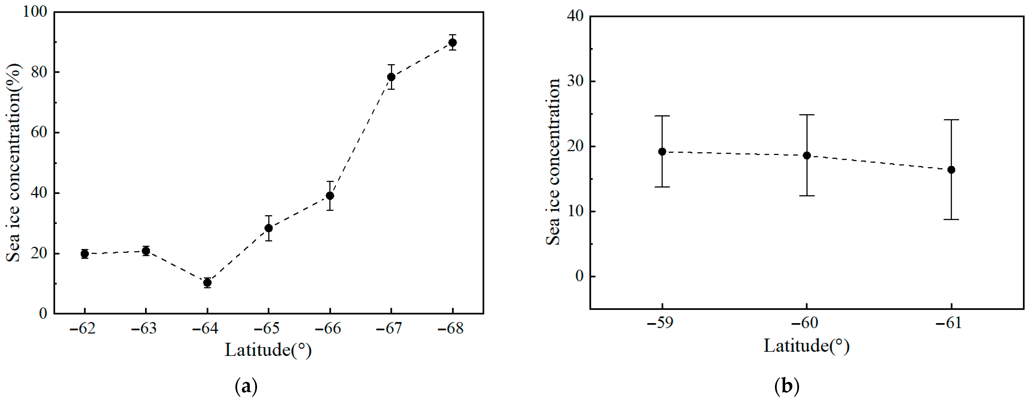
3.1.2. Spatial Distribution of SIC

To verify the difference in SIC between shipborne observation and remote sensing data at the marginal ice zone during the cruise, a spatial map showing concentration changes with latitude and longitude is presented, along with observations of the specific sea areas where sea ice appeared during the voyage (Figure 12). During the 39th Antarctic expedition, except for the stage of approaching and leaving the Zhongshan Station (62°S–68°S, 16°E–78°E), continuous sea ice appeared only in the sea area near the southeastern part of the Atlantic Ocean (59°S–61°S, 3°W–27°W), with localized areas of high SIC appearing around 18 December 2022. As discussed in Section 2.3, in order to improve navigation efficiency, the voyage avoided navigating in a high concentration region, suggesting that the sea area along the route on 18 December 2022 corresponds to the marginal ice zone. Therefore, shipborne observation data for the 18 December 2022 route area were compared with remote sensing data in Figure 13. The comparison reveals a more pronounced difference between the two data sources at the marginal ice zone and highlights the advantage of shipborne observation data. Additionally, the color variations in the concentration data points in Figure 12 illustrate differences in SIC across latitudes, indicating the need for further analysis of the concentration trend with latitude to assess the extent of sea ice coverage at each latitude.

To analyze the trend of SIC with latitude and observe the extent of sea ice coverage at each latitude, the concentration variation along the latitude is provided for the sea area close to the Zhongshan Station (where SIC is high) and the southeastern part of the Atlantic Ocean, as shown in Figure 14. The two regions exhibit different trends in SIC with latitude. Near the Zhongshan Station, the concentration trend decreases with latitude in two stages. The first stage, from 62°S to 64°S, SIC exhibited low values with no discernible spatial trend. Icebreaker navigation in this region encountered minimal resistance, indicating negligible operational impact. In the second stage, the concentration values show a pronounced increase from 64°S to 68°S, with an overall increase of about 40% between 66°S and 67°S. The average SIC close to the Zhongshan Station reaches 90%, rendering conventional vessel navigation infeasible without icebreaker support. In the southeastern part of the Atlantic Ocean, the SIC decreases slightly with latitude, remaining stable at 15–25%. In this navigational environment, conventional vessels have to make adjustments to the route.

3.1.3. Statistical Properties of SIC

The previous analysis focuses primarily on the distribution and trends of SIC under varying operational conditions and across different regions. However, the duration of the ship’s navigation in the ice-covered areas is also a critical factor influencing the strength and stability of the ship’s hull. In high-concentration ice areas, the longer the ship spends navigating, the greater the fatigue damage may be caused to the hull. Therefore, this study presents a frequency distribution graph of SIC, analyzing the concentration levels and calculating the percentage of time spent at different SIC throughout the entire voyage, as shown in Figure 15. The frequency distribution histogram exhibits a bimodal distribution. The first peak occurs within the interval [0, 10%], indicating low SIC, where the ship can navigate freely. This concentration accounts for approximately 63.0% of the total voyage time, corresponding to roughly 20 days of icebreaker navigation. This observed phenomenon primarily results from the Xuelong 2′s operational strategy during its voyage, which focused on conducting cargo resupply operations for Zhongshan and Great Wall Stations while deliberately avoiding regions with high SIC to optimize navigation efficiency. The second peak occurs within the interval [90%, 100%], indicating that the vessel required repeated icebreaking maneuvers in this concentration range. This concentration accounts for approximately 18.9% of the total voyage, corresponding to about 6 days of icebreaker navigation. This data primarily reflects the sea ice coverage observed during the Xuelong 2’s approach to the Zhongshan Station.

3.2. Results and Analysis of SIT Extraction

SIT is a critical factor in determining the icebreaking class of an icebreaker and serves as an important data reference for icebreaker design. However, research on SIT is relatively limited, and the accuracy remains difficult to verify. Therefore, this paper statistically analyzes SIT data obtained through deep learning recognition, aiming to provide a data reference for validating remote sensing data and informing ship design. Similar to the analysis of SIC in Section 3.1, the mooring period is neglected from the analysis of SIT data in this chapter.

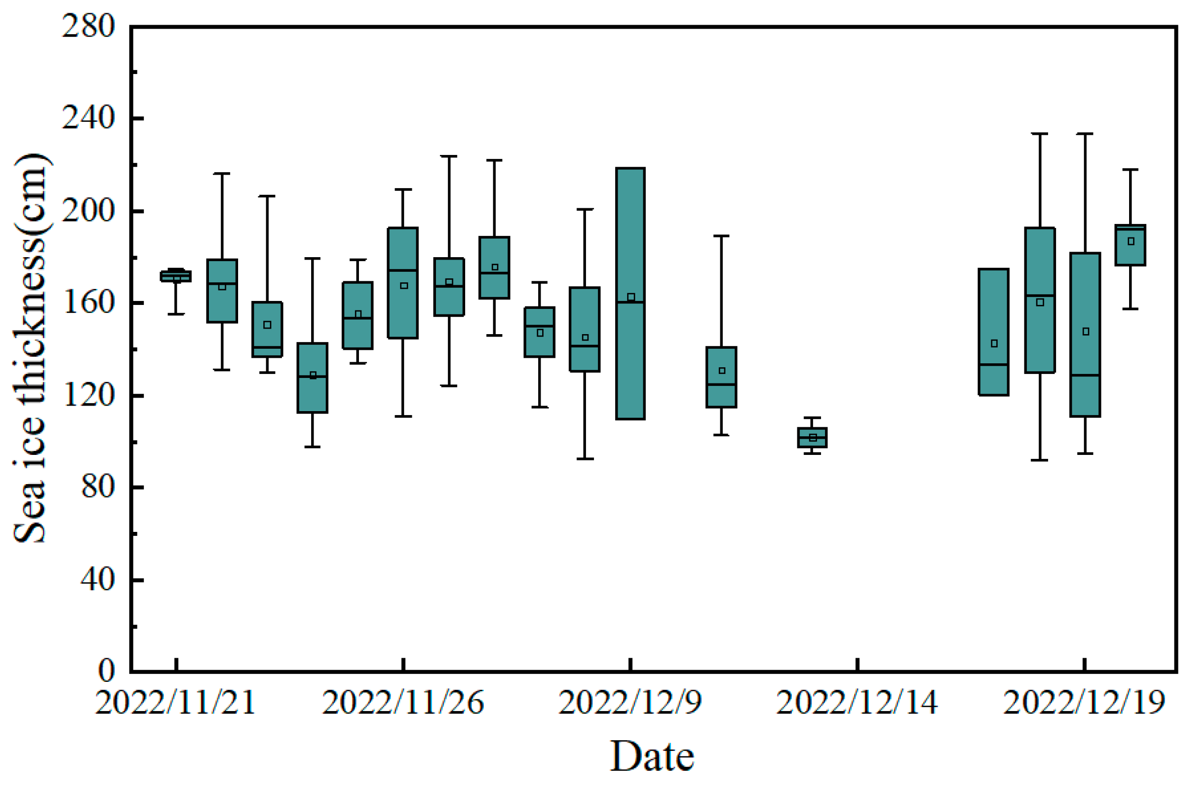
3.2.1. Temporal Distribution of SIT

Shipborne observations of SIT are primarily obtained by flipped ice cross-sections captured by the icebreaker’s camera during its voyage. These cross-sections only appear in 33.2% (17 days) of the voyage stage from the Zhongshan Station to the Great Wall Station. To study the SIT distribution, a box plot of the time history is shown in Figure 16. In general, excluding the case of traveling through open water without ice, the SIT along the voyage route was predominantly distributed between 100 and 220 cm. The minimum SIT was 92.1 cm, and the maximum thickness was 234 cm. As shown in Figure 16, the SIT exhibited a decreasing and then increasing trend as the icebreaker approached the Zhongshan Station. After leaving the Zhongshan Station, no specific trend in SIT was observed. Therefore, further analysis of SIT variations in different regions should consider the spatial distribution of sea ice.

3.2.2. Spatial Distribution of SIT

Antarctic scientific research primarily focuses on logistics and astronomical observations, which results in relatively fixed routes. As such, the spatial distribution of SIT becomes a crucial reference for determining subsequent research routes and assessing associated risks. To study the spatial distribution of SIT, the SIT distribution with respect to latitude and longitude is shown in Figure 17. The data distribution is discontinuous since the thickness can only be extracted and measured when flipped ice cross-areas are captured. Overall, SIT is primarily concentrated in two areas: near the Zhongshan Station and in the southeastern Atlantic Ocean. This distribution corresponds to the higher concentration areas discussed in Section 3.1.2, further indicating that continuous sea ice was present exclusively in these two regions during the cruise. However, the spatial distribution map only reveals the SIT distribution area. Therefore, it is essential to analyze the variation of SIT in different regions and latitudes.

This study examines the variability of SIT across different regions, plotting the intervals of SIT with latitude both close to the Zhongshan Station and in the southeastern Atlantic Ocean, as shown in Figure 18. The SIT in both regions exhibits distinct trends as latitude decreases. Near the Zhongshan Station, the SIT increases with decreasing latitude (every 2°), following an approximately geometric sequence with $\mathrm{q}={\displaystyle \frac{1}{2}}, a_1=10$. The average thickness reaches 160 cm at 68°S. In the southeastern Atlantic Ocean, due to significant longitude changes during icebreaker navigation, the average SIT decreases by approximately 25 cm for each 1° decrease in latitude, reaching 182 cm at 59°S and 128 cm at 61°S.

3.2.3. Statistical Properties of SIT

The above analysis determines the general range of SIT variation in different regions. However, for hull structure design, the primary focus should be on the overall distribution of sea ice and the proportion of different thicknesses in relation to the entire dataset. This paper will conduct a frequency concentration analysis of the entire voyage SIT dataset, revealing that the SIT follows a normal distribution with an average value of 160 ± 29.5 cm, as shown in Figure 19. Subsequently, a correlation analysis was conducted between the SIT frequency concentration and the normal distribution frequency concentration, as shown in Figure 20, showing a strong correlation. This indicates that the SIT distribution can be calculated using Formula (6), which represents the normal distribution probability concentration function.

$$f\left(x\right)={\displaystyle \frac{1}{\sqrt{2\pi }\sigma }}{e}^{-{\displaystyle \frac{{\left(x-\mu \right)}^2}{2{\sigma }^2}}}$$

(6)

where $\sigma$ denotes the average SIT for the entire voyage; $\mu$ denotes the standard deviation; and $x$ denotes a randomized value of SIT.

4. Conclusions

SIC and SIT, as key environmental parameters during ship navigation in ice-infested waters, not only influence ice resistance but also play a crucial role in evaluating sea ice conditions. In this paper deep learning method is applied to obtain sea ice parameters from shipborne camera images, which are collected during China’s 39th Antarctic Research Expedition. The following conclusions are drawn:

(1) SICs are predominantly distributed in the intervals of 0–10% and 90–100%, accounting for approximately 63% and 18.9% of the total period, respectively. High concentration is mainly observed close to the Zhongshan Station.

(2) The SIT follows a normal distribution, with the majority of values ranging from 100 to 220 cm. The average ice thickness is 160 cm, and the maximum thickness is 234 cm.

(3) Compared to satellite remote sensing data, shipborne camera data are more accurate at small-scale observations, offering higher temporal and spatial resolution. The results from the two data sources show a minimal difference in open water, with an average error of only 0.08%. However, significant discrepancies are observed in areas of ice-covered regions, with an average error of 15.5% in level ice areas and 29.7% in broken ice fields.

References

1. Cai, Q.; Wang, J.; Beletsky, D.; Overland, J.; Ikeda, M.; Wan, L. Accelerated decline of summer Arctic sea ice during 1850–2017 and the amplified Arctic warming during the recent decades. Environ. Res. Lett. 2021, 16, 034015. [Google Scholar] [CrossRef]
2. Sun, X.; Lv, T.; Sun, Q.; Ding, Z.; Shen, H.; Gao, Y.; He, Y.; Fu, M.; Li, C. Analysis of Spatiotemporal Variations and Influencing Factors of Sea Ice Extent in the Arctic and Antarctic. Remote Sens. 2023, 15, 5563. [Google Scholar] [CrossRef]
3. Copernicus Marine Service. Copernicus Marine Service Website. 2023. Available online: https://climate.copernicus.eu/climate-indicators/sea-ice#c6146155-6091-4dff-b07d-f1562e6b2989 (accessed on 30 July 2025).
4. Sahoo, S.K.; Momin, I.M.; George, J.P.; Prasad, V.S. Variability of sea ice concentration over Antarctica during recent decade. J. Earth Syst. Sci. 2025, 134, 1–13. [Google Scholar] [CrossRef]
5. Deng, L.J.; Jin, B.W.; Quan, M.Y.; Wang, A.M.; Fan, W.J.; Wang, H. Analysis of changes in Arctic sea ice and its influencing factors during 1979–2022. Mar. Inf. Technol. Appl. 2024, 39, 8–16. (In Chinese) [Google Scholar]
6. Parkinson, C.L.; DiGirolamo, N.E. Sea ice extents continue to set new records: Arctic, Antarctic, and global results. RSE 2021, 267, 112753. [Google Scholar] [CrossRef]
7. Maksym, T. Arctic and Antarctic sea ice change: Contrasts, commonalities, and causes. Annu. Rev. Mar. Sci. 2019, 11, 187–213. [Google Scholar] [CrossRef]
8. Wang, J.; Yang, Q.; Yu, L.; Song, M.; Luo, H.; Shi, Q.; Li, X.; Min, C.; Liu, J. A review on Antarctic sea ice change and its climate effects. Acta Oceanol. Sin. 2021, 43, 11–22. [Google Scholar] [CrossRef]
9. Willis, M.D.; Lannuzel, D.; Else, B.; Angot, H.; Campbell, K.; Crabeck, O.; Delille, B.; Hayashida, H.; Lizotte, M.; Loose, B.; et al. Polar oceans and sea ice in a changing climate. Elementa 2023, 11, 00056. [Google Scholar] [CrossRef]
10. Kusahara, K.; Tatebe, H.; Hajima, T.; Saito, F.; Kawamiya, M. Antarctic Sea Ice Holds the Fate of Antarctic Ice-Shelf Basal Melting in a Warming Climate. J. Clim. 2023, 36, 713–743. [Google Scholar] [CrossRef]
11. Fraser, A.D.; Wongpan, P.; Langhorne, P.J.; Klekociu, A.R.; Kusahara, K.; Lannuzel, D.; Massom, R.A.; Meiners, K.M.; Swadling, K.M.; Atwater, D.P.; et al. Antarctic Landfast Sea Ice: A Review of Its Physics. Rev. Geophys. 2023, 61, e2022RG000770. [Google Scholar] [CrossRef]
12. Eayrs, C.; Li, X.C.; Raphael, M.N.; Holland, D.M. Rapid decline in Antarctic sea ice in recent years hints at future change. Nat. Geosci. 2021, 14, 460–464. [Google Scholar] [CrossRef]
13. Tewari, K.; Mishra, S.K.; Salunke, P.; Ozawa, H.; Dewan, A. Potential effects of the projected Antarctic sea-ice loss on the climate system. Clim Dyn. 2023, 60, 589–601. [Google Scholar] [CrossRef]
14. Ren, Z.; Zha, E.; Long, H.; Liu, W. Ground penetrating radar for detecting ice cracks and crevasses in Chinese national Antarctic research expedition. Prog. Geophys. 2017, 32, 898–901. [Google Scholar] [CrossRef]
15. Huang, L.; Li, Z.; Ryan, C.; Ringsberg, J.; Pena, B.; Li, M.; Ding, L.; Thomas, G. Ship resistance when operating in floating ice floes: Derivation, validation, and application of an empirical equation. Mar. Struct. 2021, 79, 103057. [Google Scholar] [CrossRef]
16. Zhang, X.; Yu, B.; Yang, D.; Liu, L.; Ji, S. Influence of ice floe size on ice resistance of ship hull in broken ice field based on discrete element analysis. Chin. J. Comput. Mech. 2024, 41, 915–920. [Google Scholar] [CrossRef]
17. Yan, Q.; Huang, W. Sea Ice Remote Sensing Using GNSS-R: A Review. Remote Sens. 2019, 11, 2565. [Google Scholar] [CrossRef]
18. Yuan, S.; Liu, C.Y.; Liu, X.Q.; Chen, Y.; Zhang, Y.J. Research advances in remote sensing monitoring of sea ice in the Bohai sea. Earth Sci. Inform. 2021, 14, 1729–1743. [Google Scholar] [CrossRef]
19. MacGregor, J.A.; Boisvert, L.N.; Medley, B.; Petty, A.A.; Harbeck, J.P.; Bell, R.E.; Blair, J.B.; Blanchard-Wrigglesworth, E.; Buckley, E.M.; Christoffersen, M.S.; et al. The Scientific Legacy of NASA’s Operation IceBridge. Rev. Geophys. 2021, 59, 2. [Google Scholar] [CrossRef]
20. Haas, C. Evaluation of ship-based electromagnetic-inductive thickness measurements of summer sea-ice in the Bellingshausen and Amundsen Seas, Antarctica. Cold Reg. Sci. Technol. 1998, 27, 1–16. [Google Scholar] [CrossRef]
21. Uto, S.; Toyota, T.; Shimoda, H.; Tateyama, K.; Shirasawa, K. Ship-borne electromagnetic induction Sounding of Sea-ice thickness in the Southern Sea of Okhotsk. Ann. Glaciol. 2006, 44, 253–260. [Google Scholar] [CrossRef]
22. Zhou, Y.; Gong, C.L.; Hu, Y.; Meng, P.; Ma, W.W. Automatic identification and tracking the Arctic sea ice based on sequential images of FY-3A satellite. In Proceedings of the 5th International Symposium on Photoelectronic Detection and Imaging, Beijing, China, 25–27 June 2013; pp. 418–427. [Google Scholar] [CrossRef]
23. An, J.B.; Shuai, L. A BP neural network model for the sea ice recognition using SAR image. In Proceedings of the International Symposium of Remote Sensing and Space Technology for Multidisciplinary Research and Applications, Beijing, China, 19–24 May 2006; pp. 1–8. [Google Scholar] [CrossRef]
24. Su, H.; Wang, Y.; Xiao, J.; Yan, X.H. Classification of MODIS images combining surface temperature and texture features using the Support Vector Machine method for estimation of the extent of sea ice in the frozen Bohai Bay, China. Int. J. Remote Sens. 2015, 36, 2734–2750. [Google Scholar] [CrossRef]
25. Zhang, M.; Lu, X.; Zhang, X.; Zhang, T.; Wu, L.; Wang, J.; Zhang, X. Research on SVM sea ice classification based on texture features. Acta Oceanol. Sin. 2018, 40, 149–156. [Google Scholar] [CrossRef]
26. Zhang, N.; Wu, Y.S.; Zhang, Q.H. Detection of sea ice in sediment laden water using MODIS in the Bohai Sea: A CART decision tree method. Int. J. Remote Sens. 2015, 36, 1661–1674. [Google Scholar] [CrossRef]
27. Zakhvatkina, N.; Smirnov, V.; Bychkova, I. Satellite SAR data-based sea ice classification: An overview. Geosciences 2019, 9, 152. [Google Scholar] [CrossRef]
28. Boulze, H.; Korosov, A.; Brajard, J. Classification of Sea Ice Types in Sentinel-1 SAR Data Using Convolutional Neural Networks. Remote Sens. 2020, 12, 2165. [Google Scholar] [CrossRef]
29. Han, Y.; Liu, Y.; Hong, Z.; Zhang, Y.; Yang, S.; Wang, J. Sea Ice Image Classification Based on Heterogeneous Data Fusion and Deep Learning. Remote Sens. 2021, 13, 592. [Google Scholar] [CrossRef]
30. Khaleghian, S.; Ullah, H.; Kræmer, T.; Hughes, N.; Eltoft, T.; Marinoni, A. Sea Ice Classification of SAR Imagery Based on Convolution Neural Networks. Remote Sens. 2021, 13, 1734. [Google Scholar] [CrossRef]
31. Xu, G.B.; Zhao, G.Y.; Yin, L.; Yin, Y.X.; Shen, Y.L. A CNN-based Edge Detection Algorithm for Remote Sensing Image. In Proceedings of the 20th Chinese Control and Decision Conference, Yantai, China, 2–4 July 2008; pp. 2558–2561. [Google Scholar] [CrossRef]
32. Ronneberger, O.; Fischer, P.; Brox, T. U-Net: Convolutional Networks for Biomedical Image Segmentation. In Proceedings of the International Conference on Medical Image Computing and Computer-Assisted Intervention, Munich, Germany, 5–9 October 2015; Springer: Berlin/Heidelberg, Germany; pp. 234–241. [Google Scholar] [CrossRef]
33. Badrinarayanan, V.; Kendall, A.; Cipolla, R. SegNet: A Deep Convolutional Encoder-Decoder Architecture for Image Segmentation. IEEE Trans. Pattern Anal. Mach. Intell. 2017, 39, 2481–2495. [Google Scholar] [CrossRef]
34. Nagi, A.S.; Kumar, D.; Sola, D.; Scott, K.A. RUF: Effective Sea Ice Floe Segmentation Using End-to-End RES-UNET-CRF with Dual Loss. Remote Sens. 2021, 13, 2460. [Google Scholar] [CrossRef]
35. Mei, H.; Lu, P.; Wang, Q.K.; Cao, X.W.; Li, Z.J. Study of the Spatiotemporal Variations of Summer Sea Ice Thickness in the Pacific Arctic Sector Based on Shipside Images. Chin. J. Polar Res. 2021, 33, 37–48. [Google Scholar] [CrossRef]
36. Dowden, B.; De Silva, O.; Huang, W.M.; Oldford, D. Sea Ice Classification via Deep Neural Network Semantic Segmentation. IEEE Sens. J. 2021, 21, 11879–11888. [Google Scholar] [CrossRef]
37. Zhang, C.Q.; Chen, X.D.; Ji, S.Y. Semantic image segmentation for sea ice parameters recognition using deep convolutional neural networks. Int. J. Appl. Earth Obs. Geoinf. 2022, 112, 102885. [Google Scholar] [CrossRef]
38. Alsharay, N.M.; Chen, Y.Z.; Dobre, O.A.; Silva, O.D. Improved Sea-Ice Identification Using Semantic Segmentation With Raindrop Removal. IEEE Access 2022, 10, 21599–21607. [Google Scholar] [CrossRef]
39. Lin, J.T.; Peng, J.W. Adaptive inverse perspective mapping transformation method for ballasted railway based on differential edge detection and improved perspective mapping model. Digit. Signal Process. 2023, 135, 103944. [Google Scholar] [CrossRef]
40. Huang, Y.P.; Li, Y.W.; Hu, X.; Ci, W.Y. Lane Detection Based on Inverse Perspective Transformation and Kalman Filter. KSII Trans. Internet Inf. Syst. 2018, 12, 643–661. [Google Scholar] [CrossRef]
41. Lu, P.; Li, Z.J. A Method of Obtaining Ice Concentration and Floe Size From Shipboard Oblique Sea Ice Images. IEEE Trans. Geosci. Remote Sens. 2010, 48, 2771–2780. [Google Scholar] [CrossRef]
42. Wang, Q.K.; Li, Z.J.; Lu, P.; Lei, R.B.; Cheng, B. 2014 summer Arctic sea ice thickness and concentration from shipborne observations. Int. J. Digit. Earth 2019, 12, 931–947. [Google Scholar] [CrossRef]
43. Liu, D.N.; Jiang, S.Q.; Liu, G.M.; Xiang, H.H.; Liu, Z.G. Detection and Control of Surface Scar of Aircraft Rivet Based on Image Processing. In Proceedings of the Conference on Control and Its Applications (CT), Chengdu, China, 19–21 June 2019; pp. 91–97. [Google Scholar]
Figure 1. Overall structure of Ice-Deeplab network.
Remotesensing 17 02685 g001
Figure 2. Schematic diagram of the concentration algorithm. (a) Original images; (b) diagram of segmentation results; (c) original image after correction; (d) segmentation results after correctiong.
Remotesensing 17 02685 g002
Figure 3. Schematic diagram of projection conversion.
Remotesensing 17 02685 g003
Figure 4. Overall structure of U-Net model network.
Remotesensing 17 02685 g004
Figure 5. Schematic diagram of deep learning-based SIT recognition. (a) Original images; (b) deep learning segmentation results; (c) thickness determination.
Remotesensing 17 02685 g005
Figure 6. Time history of recognized ice thickness during the flipping process of a single sea ice floe.
Remotesensing 17 02685 g006
Figure 7. SIT segmentation results at different times. (a) t1; (b) t2; (c) t3. All ice blocks are marked with red boxes while the ice block selected for determining thickness is marked with yellow box.
Remotesensing 17 02685 g007
Figure 8. Schematic diagram of camera, ice flip section location, and sea level.
Remotesensing 17 02685 g008
Figure 9. The route of 39th Antarctic Expedition and Distribution of Stations.
Remotesensing 17 02685 g009
Figure 10. SIC for the 39th Antarctic Scientific Expedition.
Remotesensing 17 02685 g010
Figure 11. Time histories of SIC under different typical conditions. (a) From open water to ice area (23 November 2022); (b) in the ice area (26 November 2022); (c) from ice area to open water (7 December 2022); (d) in open water (28 December 2022).
Remotesensing 17 02685 g011aRemotesensing 17 02685 g011b
Figure 12. Spatial variation of SIC during the 39th Antarctic Expedition.
Remotesensing 17 02685 g012
Figure 13. Comparison of SIC satellite remote sensing results and shipborne observation results (18 December 2022).
Remotesensing 17 02685 g013
Figure 14. SIC versus latitude. (a) Near the Zhongshan Station; (b) South-eastern Atlantic Ocean.
Remotesensing 17 02685 g014
Figure 15. Frequency distribution of sea ice concentration.
Remotesensing 17 02685 g015
Figure 16. SIT for the 39th Antarctic Scientific Expedition.
Remotesensing 17 02685 g016
Figure 17. Spatial variation in SIT during the 39th Antarctic Research Expedition.
Remotesensing 17 02685 g017
Figure 18. SIT versus latitude. (a) Near the Zhongshan Station; (b) South-eastern Atlantic Ocean.
Remotesensing 17 02685 g018
Figure 19. Frequency distribution of SIT during the 39th Antarctic Scientific Expedition.
Remotesensing 17 02685 g019
Figure 20. Correlation analysis of SIT frequency concentration with normal distribution frequency density.
Remotesensing 17 02685 g020