Beyond the Backbone: A Quantitative Review of Deep-Learning Architectures for Tropical Cyclone Track Forecasting

Abstract

Accurate forecasting of tropical cyclone (TC) tracks is critical for disaster preparedness and risk mitigation. While traditional numerical weather prediction (NWP) systems have long served as the backbone of operational forecasting, they face limitations in computational cost and sensitivity to initial conditions. In recent years, deep learning (DL) has emerged as a promising alternative, offering data-driven modeling capabilities for capturing nonlinear spatiotemporal patterns. This paper presents a comprehensive review of DL-based approaches for TC track forecasting. We categorize all DL-based TC tracking models according to the architecture, including recurrent neural networks (RNNs), convolutional neural networks (CNNs), Transformers, graph neural networks (GNNs), generative models, and Fourier-based operators. To enable rigorous performance comparison, we introduce a Unified Geodesic Distance Error (UGDE) metric that standardizes evaluation across diverse studies and lead times. Based on this metric, we conduct a critical comparison of state-of-the-art models and identify key insights into their relative strengths, limitations, and suitable application scenarios. Building on this framework, we conduct a critical cross-model analysis that reveals key trends, performance disparities, and architectural tradeoffs. Our analysis also highlights several persistent challenges, such as long-term forecast degradation, limited physical integration, and generalization to extreme events, pointing toward future directions for developing more robust and operationally viable DL models for TC track forecasting. To support reproducibility and facilitate standardized evaluation, we release an open-source UGDE conversion tool on GitHub.

1. Introduction

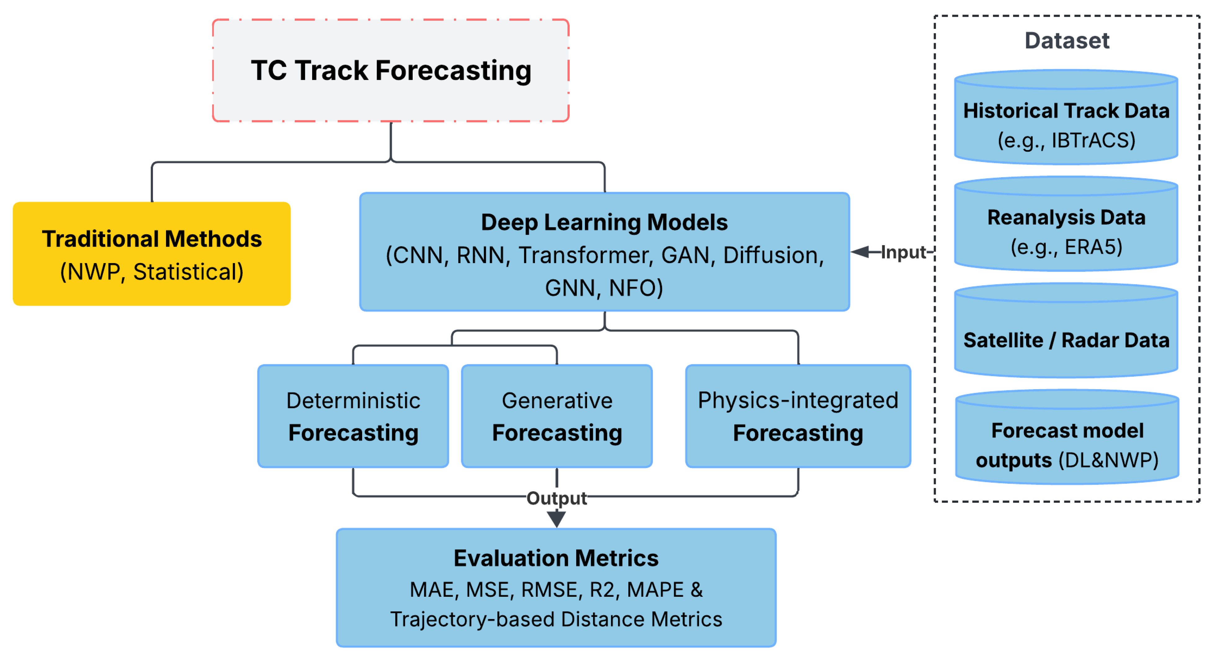
Tropical cyclones (TCs) are among the most devastating natural disasters, responsible for extensive economic damage, loss of life, and disruption of infrastructure in many coastal and island regions [1]. Accurate prediction of TC tracks, including their timing and geographical path, is critical for early warning systems, evacuation planning, and disaster mitigation. Traditional numerical weather prediction (NWP) systems have long served as the foundation of operational TC forecasting. These models simulate physical atmospheric processes through the solution of complex partial differential equations. Although NWP models offer high-fidelity forecasts, they are computationally intensive and sensitive to initial condition uncertainties [2].

In recent years, forecasting TC using AI approaches has emerged as a powerful alternative to traditional methods, with deep learning (DL) proving to be the most effective among them. Unlike NWP models, DL-based approaches can learn nonlinear spatiotemporal dependencies directly from historical data, enabling faster and potentially more robust predictions [3]. A variety of DL architectures have been explored for modeling TC behavior, including recurrent neural networks (RNNs) [4], long short-term memory (LSTM) networks [5], gated recurrent units (GRUs) [6], convolutional neural networks (CNNs) [7], Transformer models [8], graph neural networks (GNNs) [9], generative adversarial networks (GANs) [2,10,11], Fourier neural operators (FNO) [12], and diffusion models [13,14]. These models show promise in capturing the dynamic and complex evolution of TC trajectories from satellite, reanalysis, and other observational data.

A number of recent reviews have explored the application of machine learning or deep learning to TC prediction, including Wang et al. [15], Chen et al. [16], Wang and Li [17], Fan et al. [18], and others. However, this review differs significantly from prior studies in terms of scope, classification methodology, technical depth, and the standardization of evaluation criteria.

First, in terms of research domain, most previous surveys focus on general TC forecasting or even broader weather prediction tasks [19,20]. For example, Fan et al. [18], Wang et al. [15] and Chen et al. [16] present comprehensive overviews that span multiple objectives, such as TC genesis, intensity, and track, as well as associated hazards like precipitation and storm surge [1,21]. Similarly, Wang et al. [17] emphasize infrared-based TC intensity estimation, and several other reviews address sensor-based detection, radar-based diagnosis, or environmental data fusion [22]. Due to their broad scope, these reviews tend to cover only a small number of studies on TC track forecasting, often only a few representative examples, without offering a systematic model-level comparison. In contrast, our work is the first to systematically and exclusively focus on DL-based TC track forecasting, which remains underexplored in the literature despite its critical operational relevance.

Second, most existing reviews employ task-based or data-oriented taxonomies, grouping studies by forecasting objective (e.g., intensity vs. track) or input modality (e.g., infrared, reanalysis, radar). While intuitive, these approaches often obscure the technical evolution of deep-learning models. We instead adopt an architecture-centric classification, organizing the literature by DL paradigm—recurrent networks (RNNs), convolutional networks (CNNs), Transformer and graph-based models, generative frameworks (e.g., GANs, Diffusion models), and spectral operators (e.g., AFNO, SFNO). The proposed design-oriented taxonomy supports a more structured analysis of model development, enables direct comparisons, and elucidates how different deep-learning strategies are adapted for TC track forecasting.

Third, the architecture temporal coverage of prior surveys is often limited. Most conclude with traditional architectures like CNNs, LSTMs, and early GANs, rarely including more recent advances such as Swin Transformers, spatiotemporal GNNs, autoregressive Fourier neural operators, or diffusion-based models. For example, Chen et al. [16] cover GANs only up to 2020, and even the most up-to-date review we identified [15] does not incorporate developments beyond 2022. In contrast, our review explicitly includes state-of-the-art models introduced in recent years, capturing the latest trends in DL-based spatiotemporal modeling for TC track forecasting.

Finally, and most critically, existing reviews offer limited information on model performance due to inconsistent evaluation metrics. Reported errors vary widely between studies, with metrics that include mean absolute error (MAE), root mean square error (RMSE), mean absolute percentage error (MAPE), and coordinate-wise angular deviations. This heterogeneity undermines any meaningful cross-model comparison and hinders progress in benchmarking, tuning, or deployment of DL models. Unified or quantitative assessments are needed.

In this review, we focus on the emerging role of DL in the prediction of the TC track and aim to provide a critical and structured comparison of recent developments. We begin by surveying key aspects of existing DL-based models, including their architectures, input variables, data sources, prediction strategies, and evaluation metrics. In addition, we propose a unified metric, Unified Ground Distance Error (UGDE), to facilitate standardized comparison between different studies. To support practical adoption and reproducibility, we also provide an open-source tool, UGDE-Converter, that converts commonly reported error metrics (e.g., RMSE, MAE, coordinate differences) into the UGDE framework. We further examine how architectural design choices influence forecast accuracy, providing a deeper insight into the factors driving model behavior. This enables us not only to synthesize the existing literature but also to uncover key opportunities and challenges in current DL-based TC track forecasting research.

To conduct this review, we performed a systematic literature search, primarily via Google Scholar, that using keyword combinations such as “tropical cyclone,” “hurricane,” or “typhoon” in conjunction with “track,” “trajectory,” “forecasting,” or “prediction,” and “deep learning,” “machine learning,” or “artificial intelligence.” We included studies published since 2020 that focus explicitly on DL-based approaches to TC track forecasting, along with one 2019 precursor study [2] to a 2022 follow-up [10]. Traditional ML models (e.g., random forests, Support Vector Machines (SVMs)) and purely physics-based methods were excluded unless they incorporated DL components in a hybrid framework. The selected models were then curated and categorized according to architectural family, input design, and forecasting strategy. To enable standardized performance analysis, we extracted reported results and converted them into a unified UGDE metric, allowing for the first direct comparison of forecasting accuracy across diverse model types, datasets, and lead times. This process also enabled us to trace the evolution of architectural choices over time, identify recurring challenges, and highlight future research opportunities.

In summary, the main contributions of this review are:

• We present the first standardized cross-model performance comparison of DL-based TC track forecasting models, grouped by architectural paradigm, enabling in-depth analysis of architectural effectiveness across datasets and lead times.
• We introduce a unified metric (UGDE) for model evaluation and release an open-source tool, UGDE-Converter, on GitHub (https://github.com/Deepfake-H/A-Quantitative-Review-of-Deep-Learning-Architectures-for-Tropical-Cyclone-Track-Forecasting (accessed on 29 June 2025)) to support reproducible and consistent benchmarking.
• We identify key trends, strengths, and limitations across major model families through unified evaluation, revealing how architectural choices and input designs influence predictive performance. We also outline future research directions for developing more accurate, robust, and interpretable deep-learning (DL)-based forecasting systems.

The remainder of this paper is structured as follows. Section 2 introduces the fundamental concepts of TC motion and forecasting, covering both traditional NWP methods and emerging DL strategies. Section 3 categorizes and analyzes major DL architectures applied to TC track prediction. Section 4 presents a critical comparison of model performance using the UGDE metric, supported by in-depth architectural analyses. Section 5 discusses persistent challenges and outlines future research opportunities for advancing DL-based TC forecasting. Finally, Section 6 concludes the paper by summarizing the main findings and emphasizing the contributions of this review.

2. Preliminaries

This section lays the conceptual foundation for understanding DL-based approaches to TC track forecasting. We begin by introducing the fundamental characteristics of TCs and the importance of accurate track prediction. We then review traditional forecasting methods based on NWP and statistical models. Next, we highlight the growing role of DL architectures in TC track forecasting, discussing the key models employed in recent studies. To support these models, we summarize the major datasets commonly used as inputs, including historical best-track data, reanalysis data, and satellite observations. We also categorize the forecasting strategies adopted in DL-based workflows, such as autoregressive, direct, and hybrid AI-NWP prediction schemes. Finally, we review the evaluation metrics used in the literature and emphasize the need for standardized definitions to enable meaningful model comparisons. An overview of the forecasting pipeline is illustrated in Figure 1, which contextualizes the relationships between traditional and DL-based methods, input datasets, prediction strategies, and performance evaluation.

2.1. Fundamentals of TC Track Forecasting

TCs are intense, rotating storm systems that generally originate over warm ocean waters and are characterized by low-pressure centers, strong winds, and heavy rainfall [23]. These systems can cause widespread damage due to strong winds, storm surges, and inland flooding, particularly during landfall. As one of the most devastating natural disasters, TCs pose significant threats to human life, infrastructure, and ecosystems across tropical and subtropical regions [24].

TC track forecasting refers to the task of predicting the future geographic positions of a cyclone over time, based on historical observations, environmental data, and atmospheric dynamics [25]. Accurate track forecasts are crucial for early warning systems, evacuation planning, and disaster risk reduction. The movement of TCs is primarily governed by large-scale environmental steering flows, beta drift, the Coriolis force, and interactions with landmasses or other synoptic-scale systems [26,27]. Even small errors in track prediction can lead to substantial uncertainty in identifying affected regions, underscoring the need for continued improvements in forecasting methodologies.

2.2. Traditional Approaches to TC Track Forecasting

NWP models simulate physical atmospheric processes through the solution of partial differential equations, providing high-accuracy forecasts at the cost of substantial computational resources [28]. Additionally, NWP models are sensitive to initial conditions and model resolution, which can lead to significant forecast errors, especially in rapidly evolving systems like tropical cyclones. Their performance is also constrained by inherent uncertainties in physical parameterizations and boundary conditions [29]. In contrast, statistical and statistical-dynamical methods employ regression techniques, analog approaches, or simplified physical representations to approximate TC motion, typically sacrificing some accuracy in favor of computational efficiency [30,31].

2.3. Deep Learning in TC Track Forecasting

DL, a subfield of machine learning within the broader domain of artificial intelligence (AI), leverages deep neural networks to learn hierarchical representations from data [3].

In the context of TC track forecasting, DL has become the dominant approach due to its capability in modeling spatiotemporal dependencies in geophysical data.

Common DL architectures include:

• Recurrent Neural Networks (RNNs): e.g., LSTM and GRU, suitable for sequence prediction [5,6].
• Convolutional Neural Networks (CNNs): effective in extracting spatial features from meteorological fields [7,32].
• Transformer-based models and graph neural networks (GNN): useful for long-term dependencies and spatial relationships [9].
• Generative Models (GANs, Diffusion Models): support probabilistic and ensemble-style forecasting [10,11].
• Fourier-based Neural Operators (FNO): performs global or regional forecasting via learned frequency-domain transformations [12].

In this work, we focus on recent DL models, especially those based on neural networks, as the core of AI-driven approaches for TC track forecasting, without including earlier machine learning techniques such as Random Forests or SVMs.

2.4. Datasets for DL-Based TC Track Forecasting

Historical TC track datasets: The International Best-Track Archive for Climate Stewardship (IBTrACS) project is the most complete global collection of tropical cyclones available. It merges recent and historical tropical cyclone data from multiple agencies to create a unified, publicly available, best-track dataset that improves inter-agency comparisons. IBTrACS was developed collaboratively with all the World Meteorological Organization (WMO) Regional Specialized Meteorological Centers, as well as other organizations and individuals from around the world. IBTrACS provides latitude, longitude, maximum sustained wind speed, and minimum central pressure at regular intervals (typically 6-hourly) for TCs in history [33]. This dataset forms the foundation for model training, validation, and performance evaluation in track forecasting. Other widely used track datasets include the China Meteorological Administration Best-Track dataset (CMA-BST) [32], the Joint Typhoon Warning Center Best-Track dataset (JTWC) [34], and NOAA’s HURSAT-B1 dataset [35] spans from 1978 to present, while the HURDAT2 dataset [36] covers the period from 1851 to present; both provide cyclone specific variables such as USA_LAT, USA_LON, and USA_WIND, which are commonly used for both track and intensity prediction.

Reanalysis datasets: Reanalysis datasets are widely used in meteorological and climate research as they provide gridded, high-resolution reconstructions of the atmosphere by assimilating historical observations into a consistent numerical model framework. Two reanalysis datasets are widely used in the reviewed AI-based models. ERA5 [37], developed by the European Center for Medium-Range Weather Forecasts (ECMWF), is the fifth-generation global reanalysis dataset, providing hourly atmospheric fields (e.g., wind, temperature, pressure) at high spatial resolution from 1940 onwards. The NCEP/NCAR Reanalysis is a collaborative effort between the National Centers for Environmental Prediction (NCEP) and the National Center for Atmospheric Research (NCAR). It was one of the first large-scale efforts to produce a consistent, long-term global atmospheric dataset using data assimilation techniques [38].

Forecast model outputs: Outputs from operational NWP models are often used as baselines or auxiliary inputs in AI models. ECMWF’s Integrated Forecasting System (IFS) provides high-resolution deterministic and ensemble forecasts for global applications [39]. The Hurricane Weather Research and Forecasting model (HWRF) [40] is a regional NWP system developed by NOAA, specifically designed for TC forecasting, offering predictions on intensity, track, and structure.

Satellite and radar observations: Satellite and radar observations serve as critical data sources and are widely utilized in AI-based TC forecasting models. Geostationary Operational Environmental Satellites (GOES) operated by NOAA deliver near-real-time visible and infrared imagery used for TC cloud structure and intensity analysis over the East Pacific and Atlantic Ocean [41], while Himawari-8 operated by Japan Meteorological Agency (JMA) provides high-frequency multi-band imagery over the Asia–Pacific region, crucial for monitoring TC evolution [42]. Scatterometers (e.g., ASCAT) supply surface wind vector data over global oceans by measuring changes in radar backscatter caused by the wind, aiding in the assessment of TC position and intensity [43]. These datasets enable the extraction of high-resolution structural features critical to TC tracking and intensity estimation.

2.5. Forecasting Strategies in DL-Based TC Prediction

2.5.1. Forecasting Horizon Strategy

DL-based TC forecasting models adopt different strategies based on the forecasting horizon and the nature of the output.

Autoregressive forecasting: predicts one step ahead at each iteration and feeds the output into the next prediction step. This allows the model to handle sequential dependencies but can lead to the accumulation of errors over longer time horizons [44].

Direct forecasting: outputs multiple future steps simultaneously, improving stability and mitigating compounding errors. Transformer-based models are especially effective for this strategy due to their global attention mechanism [45].

2.5.2. Output Nature Strategy

DL models can also be classified based on whether they produce a single deterministic path or a probabilistic distribution of possible outcomes.

Deterministic forecasting: generates a single trajectory as the predicted outcome, usually by optimizing pointwise distance metrics such as mean absolute error (MAE), Root Mean Squared Error (RMSE) [32]. This approach is prevalent due to its interpretability and ease of evaluation, but it inherently lacks uncertainty representation and may struggle with ambiguous cases or bifurcating storm paths.

Generative forecasting: models such as GANs, VAEs, or diffusion models learn to represent the distribution of future cyclone positions, enabling uncertainty quantification and multi-modal forecasting. Although these models can produce multiple possible trajectories or forecast cones, most studies still extract a single representative center point for evaluation and downstream use [11].

2.5.3. Physics-Integrated Forecasting

Some approaches integrate deep-learning models with physical knowledge, such as outputs from NWP systems or explicit physical constraints. These strategies improve consistency with dynamical principles, reduce systematic bias, and improve interpretability. Examples include using NWP fields as boundary forcing [46], embedding conservation laws in loss functions, or coupling DL modules with physical simulators.

In addition, state-of-the-art global AI weather models, such as GraphCast [9], Pangu-Weather [45], FuXi [14], and AIFS [47] are designed to predict global atmospheric states (e.g., wind, pressure, temperature) using deep-learning architectures. Although all these models belong to the class of AI-based foundation models for weather forecasting, some explicitly incorporate tropical cyclone (TC) tracking capabilities. For example, FuXi reports multiple improvements over the original ECMWF TC tracking algorithm; Pangu-Weather describes the use of its own predictions to track TCs and compares the results against ECMWF-HRES, a high-resolution (9 km × 9 km) operational TC tracking system; and AIFS explicitly states that it is capable of high-skill forecasting of upper-air variables, surface weather parameters, and tropical cyclone tracks. In contrast, GraphCast notes that different trackers were applied to GraphCast and HRES, implying that the TC trajectories are not a direct output of the model itself.

In our taxonomy, we therefore label the model’s task as “Track + Weather” if the associated publication indicates embedded or enhanced TC tracking functionality. Models that do not include such tracking capabilities and require generic post-processing are labeled as “Weather” only.

2.6. Evaluation Metrics

Despite increasing interest in DL-based TC track forecasting, there remains no standardized approach to evaluating model performance. Current studies adopt a diverse set of metrics, often inconsistently defined or ambiguously applied. Some works rely on conventional machine learning regression metrics such as Mean Squared Error (MSE), MAE, RMSE, and the coefficient of determination ($R^2$). Others use domain-specific measures based on spatial distance errors between predicted and observed cyclone positions. In many cases, the same term, for example, MAE, may refer to fundamentally different quantities, such as coordinate-wise errors in degrees or geodesic distance errors in kilometers. This inconsistency complicates direct comparison between models and may lead to misinterpretation of results.

Mean Squared Error: MSE computes the average of the squared differences between predictions and observations, e.g., [48]. By squaring the errors, it heavily penalizes larger deviations, making it sensitive to outliers. In TC forecasting, MSE is valuable for detecting large deviations that could represent severe forecast errors.

Root Mean Squared Error: RMSE is the square root of the MSE, restoring the error to the original scale of measurement, e.g., [4]. It provides a balance between capturing the overall error magnitude and emphasizing larger errors. RMSE is widely used in TC track forecasting to evaluate prediction accuracy in units like kilometers.

Coefficient of Determination ($R^2$): $R^2$ quantifies how much of the variance in the observed data is explained by the model predictions, e.g., [32,48]. An $R^2$ value close to 1 indicates high predictive skill, whereas a value near 0 suggests that the model performs no better than a mean-based forecast. Although $R^2$ does not directly represent distance error, it provides insight into overall trajectory model fitting quality.

Mean Absolute Percentage Error (MAPE): MAPE calculates the average absolute percentage difference between predictions and true values, e.g., [32,48]. It offers intuitive interpretability by expressing errors as percentages. However, for TC track forecasting, MAPE is less commonly used because the percentage error becomes unstable when true position values are near zero or small.

Mean Absolute Error: MAE is a widely used metric in AI-based TC track forecasting, measuring the average magnitude of errors between predicted and observed locations. However, its specific definition varies across studies, leading to inconsistencies in reported results. In most cases, MAE refers to the average absolute errors in latitude and longitude, expressed in degrees [35,49,50]. Some studies, however, use MAE to represent the ground distance error between predicted and true TC centers, typically calculated using great-circle distance formulas [7,14]. This ambiguity complicates direct comparisons across models.

Trajectory-based Distance Metrics: Several studies adopt error metrics that directly measure the spatial distance between predicted and observed cyclone positions. However, the terminology used to describe such errors is highly inconsistent. Reported terms include absolute error [2,10], average absolute error [11,50], average absolute position error [6], average absolute distance error [51], average prediction distance error [5], average error [48], error [8], track error [46,52], TC position error [47], median track error [9], mean direct position errors [45], APE (absolute position error) [34,35], MDE (mean distance error) [53,54], and even MAE (mean absolute error) [7,14]. These inconsistencies reflect not only differences in naming but also in how errors are calculated.

This lack of standardized terminology and metric definition presents a significant barrier to fair and transparent model comparison. For example, ref. [34] uses APE to refer to the ground distance error, which may be confused with MAPE, commonly used in other time-series forecasting tasks [32,48]. Moreover, when MAE is reported, it is often unclear whether it refers to coordinate-based errors or distance-based errors, making direct numerical comparisons misleading.

To address these issues, we later introduce a unified metric definition and provide a conversion tool to standardize commonly used evaluation formats. These efforts, presented in Section 4, aim to ensure consistency and enable fair comparisons across DL-based TC track forecasting models.

3. Deep Learning in TC Forecasting

In recent years, deep learning (DL) has emerged as a powerful alternative to traditional numerical and statistical approaches to TC track prediction. DL models can capture complex nonlinear spatiotemporal patterns from large-scale geophysical datasets without relying on explicit physical equations. This section categorizes and reviews the main classes of DL architectures applied to TC track forecasting, including RNNs and their variants, CNNs, Transformer-based models, and GNNs. It also discusses generative approaches for sequence generation and uncertainty quantification, as well as hybrid methods that incorporate physical constraints or NWP components into the DL framework.

Table 1. Comparison of DL models for TC forecasting across key architectural and methodological characteristics, sorted by model architecture.

Study	Task	Architecture	Gen.	Phy.	Datasets
[34]	T	BiGRU + Attention	⃝	✗	JTWC
[35]	T	ConvLSTM + Temporal Atte.	⃝	✗	NCEP + NCAR + HURSAT-B1
[55]	I	LSTM	⃝	✓	NCEP + NCAR + NCEP-GFS + CMA
[5]	T	LSTM + MLP	⃝	✗	IBTrACS
[48]	T	RNN/BiLSTM/GRU	⃝	✗	CMA-BST
[4]	T	RNN/GRU/LSTM	⃝	✗	SHIPS
[6]	T	GRU + AE	⃝	✗	JTWC
[7]	T	CNN + LSTM	⃝	✗	NII + Himawari-1 8 + GOES
[54]	T	CNN + BiLSTM	⃝	✗	CMA-BST + CFSR-GPH
[51]	T	CNN + GRU	⃝	✗	ERA5
[53]	T	CNN + TCN	⃝	✗	IBTrACS + ERA5
[32]	T	TCN/LSTM/ConvLSTM/Trans.	⃝	✗	CMA-BST
[56]	F	ResNet + UNet	⃝	✗	NCEP-FNL + IBTrACS
[57]	I	CNN + Contrastive	⃝	✗	GridSat-B1 + ERA5 + CMA-BST
[45]	T + W	3D Earth-specific Trans. (Pangu)	⃝	✗	ERA5
[9]	W	GNN	⃝	✗	ERA5
[47]	T + W	GNN + Transformer	⃝	✗	ERA5 + IFS
[58]	T + I + S	Transformer/GNN/SFNO/AFNO	⃝	✗	ERA5
[8]	T	Transformer	⃝	✗	CMA
[59]	I	Transformer	⃝	✗	TCIR
[60]	I	ViT	⃝	✗	TCIR
[11]	T	GAN + LSTM + UNet	●	✗	CMA-BST + ERA5
[61]	T	GAN + LSTM	●	✗	HWRF + ERA5 + CMA
[50]	T + I	GAN + LSTM	●	✗	CMA
[2]	T	GAN + CNN	●	✗	KMA + NII + ERA-interim
[10]	T + I	GAN + CNN	●	✗	KMA + ERA-interim
[62]	T	GAN + CNN	●	✗	GridSat-B1 + ERA5 + IBTrACS + BoM
[49]	I	VAE + LSTM	◐	✗	ERA5 + IBTrACS + FengWu output
[13]	S	Video Diffusion	●	✗	ERA5 + INSAT/GOES/Himawari/Meteosat
[63]	I	DDPM	●	✗	ERA5 + HWind + IBTrACS
[14]	T + W	DDPM + Transformer (Fuxi)	●	✗	ERA5 + IBTrACS
[64]	D	NeuralGCM	⃝	✓	ERA5 + WeatherBench2 + CMIP6 + X-SHiELD output
[46]	T	Pangu Transformer + WRF	⃝	✓	IBTrACS-WMO + TIGGE + NCEP-GFS + ERA5 + Freddy
[52]	T + I	Pangu Transformer + WRF	⃝	✓	ERA5 + NCEP + SAR + JTWC
[12]	W	SFNO	⃝	✗	ERA5 + SWE output

Note: ✓ = physical constraint integrated; ✗ = no physical constraint. ● = fully generative architecture (e.g., GAN, VAE, Diffusion), where generation is the dominant structure and output is sampled from learned distributions; ◐ = hybrid generative approach, where generative modules (e.g., GAN, VAE) are used in combination with non-generative models (e.g., LSTM, CNN) but not as the primary framework; ○ = no generative component present in the architecture. Task type: F = Formation of TC; T = Track of TC; W = Weather; S = Structure of TC; I = Intensity of TC; D = Density of TC; For AI global weather models, we assign the task type as T + W if the model explicitly outputs TC track predictions or includes specific modifications for the tracking algorithm. If such TC-related capabilities are not clearly stated, the task type is recorded as W only.

provides a comparative overview of representative studies, organized by task, architecture type, use of generative and physics-based elements, and datasets.

3.1. Recurrent Neural Networks (RNNs) and Variants

RNNs and their variants, such as long short-term memory (LSTM), gated recurrent units (GRU), and convolutional LSTM (ConvLSTM), have been widely used in TC forecasting tasks due to their ability to capture temporal dependencies in sequential meteorological data. Early efforts focused on leveraging temporal modeling through recurrent neural networks, with subsequent improvements that incorporate spatial and contextual information to improve prediction accuracy and interoperability. The following subsections first examine the evolution of RNN-based architectures and then discuss comparative evaluations highlighting their strengths and limitations in TC track forecasting.

Lu et al. [7] proposed DeepTyphoon, a CNN–LSTM-based framework that marks typhoon centers directly on satellite imagery. It employs hybrid dilated convolutions and a convolutional block attention module (CBAM) to improve spatiotemporal feature extraction. The model achieved a 6-h MAE of 64.17 km, outperforming conventional DL methods.

To incorporate geographical and environmental factors, Farmanifard et al. [5] introduced a context-aware hybrid model combining MLP and LSTM. By integrating internal (e.g., TC direction and speed) and external (e.g., wind speed and air pressure) contextual data, the hybrid model significantly improved long-term prediction accuracy, reducing the average 24-h track error compared to standalone models.

Building upon the need to model environmental complexity, Huang et al. [11] proposed MGTCF, a multi-generator GAN-based framework. It introduces two key innovations: a generator chooser network (GC-Net) that probabilistically selects among multiple generators, and an Environment Net (Env-Net) that explicitly encodes environmental influences. MGTCF demonstrated lower forecast errors than China’s official forecast system, particularly in 6 to 24-h prediction windows.

Lian et al. [6] addressed data imbalance and model generalization by proposing a fusion model combining an auto-encoder (AE) with a gated recurrent unit (GRU). The AE layer compresses multi-variable meteorological inputs, while the GRU models sequential dependencies. This approach showed consistent improvement over both NWP and other DL models, reducing track prediction errors by up to 56% over 72-h lead times.

Li et al. [35] focused on long-range forecasting with their TAM-CL model, which integrates ConvLSTM with three-dimensional convolution and a temporal attention mechanism. Using atmospheric reanalysis data, the model enhances the capture of spatiotemporal dynamics and achieves reduced prediction errors across 24-, 48-, and 72-h forecasts.

To further address short-term track and intensity forecasting, Huang et al. [50] proposed MMSTN, a Multi-Modal Spatial-Temporal Network. It jointly processes trajectory and intensity inputs and incorporates a Feature Updating Mechanism (FUM) and GAN module to predict a cone of probability for future TC movements. MMSTN demonstrated better accuracy than the China Central Meteorological Observatory in 6-h forecasts.

Lastly, Song et al. [34] presented a BiGRU-based model with attention, focusing on identifying the most influential historical time steps in TC trajectories. Their model surpassed traditional operational systems and DL baselines (RNN, GRU, LSTM), particularly excelling in 72-h track forecasts.

These studies demonstrate a clear evolution from basic temporal models to advanced hybrid architectures with context-awareness, attention mechanisms, and probabilistic outputs. Collectively, they highlight the promise of DL in improving short-term TC prediction.

In addition, several studies have conducted systematic comparisons among RNN architectures and other mainstream DL models in the context of TC track prediction. These comparative efforts primarily focus on assessing the forecasting accuracy, computational efficiency, and generalizability of models such as LSTM, GRU, ConvLSTM, TCN, and Transformer under various configurations and data regimes.

For example, a study [35] evaluated RNN, LSTM, and GRU on cyclone trajectory prediction in the Indian Ocean basin using the SHIPS dataset. All models were trained on the same features selected via a Chi-square test and random forest importance ranking. Results showed that LSTM consistently achieved the lowest RMSE and MADE scores, followed by GRU and RNN, across lead times up to 72 h. This study underscored the robustness of memory-gated units in sequence modeling, especially in regions with lower data density.

A similar study by Hao et al. [48] extended this comparison in the Northwest Pacific region using China Meteorological Administration (CMA) cyclone best-track data. Besides validating LSTM and GRU as superior to standard RNN, this work also examined the effects of network depth, input history length, and attention mechanisms. Their results revealed that GRU models tend to outperform LSTM in short-range predictions (e.g., 6 h), while LSTM offers better stability in medium to long-range forecasts (24–72 h). The authors also highlighted the importance of training data length and learning rate decay on model convergence.

Wang et al. [51] included GRU, LSTM, and a novel GRU-CNN hybrid model in their evaluation. Leveraging ERA5 reanalysis data alongside IBTrACS cyclone track records, their GRU-CNN fusion achieved substantially lower prediction errors across multiple time horizons compared to all baseline RNNs. The incorporation of CNN modules allowed for better spatial encoding of environmental fields, demonstrating the benefit of hybridizing sequential and spatial architectures.

A broader evaluation was presented in [32], which compared four mainstream DL architectures—LSTM, ConvLSTM, temporal convolutional network (TCN), and Transformer—on both trajectory and intensity prediction tasks. The study concluded that TCN yielded the best overall performance in 6-h forecasts, outperforming LSTM and ConvLSTM in both RMSE and MAPE. Transformer models, while computationally efficient, suffered from degraded performance due to the limited training data size, a known limitation in sequence-to-sequence attention mechanisms.

Overall, these comparative studies reinforce the general trend that gated RNN variants (LSTM and GRU) outperform standard RNNs in TC track forecasting. GRU tends to dominate in short-term prediction, whereas LSTM offers more stable performance over medium-range horizons (up to 72 h). Hybrid structures such as GRU-CNN and modern sequence models like TCN show great promise, especially when spatial dynamics and computational efficiency are key concerns.

Although RNN-based approaches for TC track prediction exhibit promising short-term accuracy and flexibility across varying input types, they remain limited in long-horizon prediction, handling sharp track changes, and integrating physical constraints.

3.2. Convolutional Neural Networks (CNNs)

CNNs are well suited for extracting spatial features from gridded meteorological data, satellite imagery, and reanalysis fields, making them valuable for vision-inspired weather prediction tasks. However, compared to RNNs, CNNs have been less widely adopted in TC track forecasting. This is largely because track forecasting is inherently sequential and depends heavily on temporal dynamics, for which RNN-based models (e.g., LSTM, GRU) are more naturally aligned. Despite this, several studies have demonstrated that when integrated with temporal models or adapted for spatiotemporal processing, CNNs can contribute significantly to TC prediction performance, particularly when multi-modal inputs and spatial context are important.

Several studies have incorporated CNNs into hybrid or standalone architectures for TC track prediction. Lu et al. [7] proposed DeepTyphoon, which combines CNNs with LSTM and CBAM attention for image-to-image prediction of TC center trajectories. By marking typhoon centers directly on satellite images and applying hybrid dilated convolutions, their model achieved a 6-h mean absolute error (MAE) of 64.17 km, outperforming existing RNN-based baselines.

Liu et al. [54] proposed DBF-Net, a dual-branched spatiotemporal fusion network that integrates an LSTM-based encoder for inherent TC features and a CNN-based encoder for 2D geopotential height fields. By effectively combining temporal and spatial features through a dual-path architecture, DBF-Net achieved a 6-h MDE of 31.30 km and a 24-h MDE of 119.05 km, significantly improving over previous deep-learning-based approaches. In addition, ablation results indicate that the CNN-based pressure-field encoder plays a dominant role in DBF-Net’s track forecasting accuracy, while the LSTM-based TC-feature encoder provides complementary temporal information that enhances short-term predictions.

Li et al. [35] introduced TAM-CL, which uses ConvLSTM and 3D temporal attention to forecast directional vectors $(\theta ,\widehat{d})$ of TC movement. The model achieved a 24-h APE of 155.04 km and a 72-h error of 365.60 km.

Huang et al. [50] developed the MMSTN framework, a multi-modal spatial-temporal model that jointly predicts TC track and intensity. It integrates a Feature Updating Mechanism (FUM) and a cone-generation GAN to output probabilistic track estimates. MMSTN outperformed the CMA official forecast in 6-h prediction windows.

Wang et al. [51] proposed the GRU_CNN model, fusing trajectory inputs with CNN-extracted features from reanalysis data such as sea-surface temperature (SST), wind, and geopotential height. Their model achieved high short-term accuracy, with 6-h and 12-h errors of 17.2 km and 43.9 km, respectively, improving over the CMA baseline.

Gan et al. [32] conducted a comparative study of multiple DL techniques, including CNN, ConvLSTM, TCN, and Transformer, for short-term TC track and intensity forecasting. Although CNNs were included, ConvLSTM and TCN outperformed in both accuracy and temporal stability, highlighting CNN’s limitations in temporal modeling.

Yang et al. [53] further extended CNN use in the MT-CNN-TCN framework, which combines 2D/3D CNNs with temporal convolutional networks (TCNs). This model captures multidimensional input patterns and time-difference series, improving 12/24/48-h prediction accuracy by 7%/13%/16% over LSTM.

Beyond track prediction, CNNs have also been successfully applied to other TC forecasting tasks such as intensity estimation, precipitation nowcasting, and rapid intensification (RI) classification. For instance, Huang et al. [11] developed the MGTCF framework using CNN encoders to process heterogeneous meteorological data, incorporating environmental signals via a dedicated environment-aware module. Sønderby et al. [65] introduced MetNet for short-term precipitation forecasting by integrating CNNs with ConvLSTM and axial attention. Similarly, Wang et al. [57] employed CNNs in a contrastive learning framework to identify structural features critical to RI prediction. While these models demonstrate the versatility of CNNs in spatial representation learning, they have not yet been effectively extended to standalone or dominant roles in TC track forecasting. This may be attributed to CNNs’ limited capacity in modeling long-range temporal dependencies, a key requirement for sequential position prediction tasks. Without integration into temporal structures or hybrid architectures, CNN-based models remain constrained in addressing the spatiotemporal complexity of cyclone track evolution.

3.3. Transformer-Based Models and Graph Neural Networks (GNNs)

Transformer and GNN architectures have become increasingly relevant in meteorological forecasting due to their strength in capturing long-range temporal dependencies and complex spatial relationships. In the context of TC prediction, several studies have begun applying these models to improve accuracy in track, intensity, and multi-modal forecasts. We classify existing literature into two groups: (1) studies developing and applying Transformer or GNN-based models to TC-related forecast tasks, and (2) comparative studies evaluating the performance of GNN models against other DL approaches.

Jiang et al. [8] use a standard Transformer network that jointly predicts TC track (latitude and longitude) and intensity by encoding temporal dynamics through multi-head self-attention and a dynamic-length input window. They noted that the Transformer achieved superior performance in the 24-h forecast, outperforming both GRU and LSTM baselines.

Several studies have proposed enhanced Transformer [45] or GNN-based models [9] tailored to TC forecasting. Bi et al. [45] developed the 3D Earth Transformer (3DEST), a spatiotemporally structured model designed to capture long-range dependencies in global geophysical fields, demonstrating strong skill in TC trajectory forecasting. Lam et al. [9] introduced GraphCast, a GNN-based global weather model using mesh-based graph convolutions for autoregressive forecasting. It demonstrated skillful TC tracking over a 10-day horizon. Similarly, ECMWF’s operational model AIFS [47] combines GNN encoders/decoders with a Transformer processor, forming a modular structure capable of global multi-step TC prediction.

Some hybrid approaches integrate enhanced Transformer models with physical components. Liu et al. [46] coupled the transformer-based Pangu-Weather model with WRF, incorporating boundary nudging and SST updates for regional track and intensity forecasts. Xiao et al. [66] further embedded FengWu into a 4DVar assimilation cycle, highlighting potential synergy between physical and AI components, though not directly evaluated for TC track prediction. Xu et al. [52] applied Pangu-initialized WRF to enhance vortex structure, focusing specifically on intensity improvements.

Beyond track prediction, Transformers have been adapted for TC intensity modeling. Chen et al. [60], Tian et al. [59], and Xu et al. [59] use multi-modal satellite fusion and multi-task learning, respectively, to estimate TC intensity from image-based inputs. While promising, these approaches have not yet been extended to spatial trajectory forecasting.

Some studies have conducted comparative evaluations of Transformer and GNN architectures against traditional RNN-based models for TC track forecasting. Jiang et al. [8] compared the Transformer with GRU and LSTM networks on a CMA dataset. The Transformer achieved the best performance across all forecast horizons (6 h to 24 h). Specifically, it reduced the 24-h track MAE to 1.15° in latitude and 1.52° in longitude, outperforming GRU and LSTM, which showed higher errors throughout.

In contrast, Gan et al. [32] evaluated four mainstream DL models—LSTM, ConvLSTM, Temporal Convolutional Network (TCN), and Transformer—under various input length and time interval configurations. Their results revealed that TCN performed best in terms of accuracy, stability, and efficiency, followed by ConvLSTM. The Transformer and LSTM models lagged behind, with the Transformer showing relatively weak predictive accuracy despite the training efficiency. In particular, under one-step and multi-step TC track prediction scenarios, TCN consistently yielded lower MAPE than the Transformer.

In a broader comparative context, Charlton-Perez et al. [58] conducted a large-scale case study of four machine learning models—FourCastNet, FourCastNet-v2, Pangu-Weather, and GraphCast—compared against the ECMWF-IFS. All ML models applied Transformer or GNN architectures. Although these models accurately reproduced the overall track of Storm Ciarán, they underrepresented wind intensity and mesoscale structures. Among the ML models, Pangu and GraphCast showed the highest skill in track prediction, suggesting their suitability for operational TC monitoring despite some limitations in representing storm intensity.

Overall, while comparative studies reveal that although Transformers can outperform RNNs in short-term forecasting, they still struggle to capture fine-grained track variations. In particular, existing research rarely focuses on outlier events or landfall TCs, both of which are critical to disaster preparedness. Enhanced Transformer-based models have shown strong potential in long-range weather forecasting; their application to TC track prediction remains limited in several respects. These models typically rely on extensive training data and require significant computational resources, which can hinder their operational scalability. Moreover, GNN-based models such as GraphCast have shown promising skill in global-scale forecasting, but their targeted application to TC track prediction remains underexplored. In summary, despite encouraging initial results, the use and evaluation of Transformer and GNN models for TC track forecasting are still in their early stages and warrant further task-specific development and analysis.

3.4. Generative Models

Recent advances in deep generative modeling have introduced powerful tools for forecasting complex geophysical phenomena such as TCs. Unlike deterministic models that produce single-point forecasts, generative approaches aim to capture the distributional uncertainty and spatial-temporal variability of atmospheric states. In the context of TC prediction, these models are particularly attractive for producing diverse trajectory scenarios, high-resolution wind structures, or long-range intensity evolution.

GANs have been widely applied to TC track forecasting tasks for their capacity to model complex spatial-temporal dynamics. Ruttgers et al. [2] proposed a multi-scale GAN architecture incorporating satellite imagery and wind fields. Their model demonstrated improved short-range trajectory prediction, with a 6-h MAE of 69.1 km when wind inputs were used, compared to 95.6 km without. Building on this approach, Ruttgers et al. [10] extended the model to jointly predict TC track and intensity using multivariate meteorological time-series. The model achieved a 6-h MAE of 44.5 km and a 12-h MAE of 68.7 km, outperforming JTWC forecasts at the corresponding lead times.

To improve short-term track and intensity forecasting, Huang et al. [50] proposed MMSTN, a Multi-Modal Spatial-Temporal Network that integrates trajectory and intensity information through an LSTM-based encoder-decoder architecture enhanced with a GAN module. The model uses a Feature Updating Mechanism and cone-of-probability prediction to capture diverse TC tendencies. MMSTN achieved track MAEs of 27.57 km (6 h), 59.09 km (12 h), and 139.19 km (24 h), outperforming baselines including CMO and Multi-LSTM. For intensity, it achieved 24 h pressure and wind errors of 4.74 hPa and 2.55 m/s, respectively. As a direct extension, the same authors later developed MGTCF [11], a multi-generator GAN framework designed to improve robustness and diversity in trajectory forecasting. MGTCF incorporates heterogeneous meteorological inputs and an environment-aware encoding module (Env-Net), along with a generator chooser network (GC-Net). It achieved lower trajectory errors of 23.14 km (6 h) and 93.08 km (24 h), and significantly outperformed MMSTN and CMO in intensity forecasting.

Li et al. [61] proposed AST-GAN, an attention-enhanced spatiotemporal GAN framework designed to improve TC track forecasting. The model integrates a spatiotemporal LSTM generator with a multi-scale discriminator and incorporates a channel attention mechanism to enhance feature representation. Trained on HWRF forecast data and fine-tuned with ERA5 reanalysis, AST-GAN achieved promising trajectory accuracy in case studies, including a track prediction error of 41.16 km. In addition, the model demonstrated strong performance in forecasting wind fields, achieving RMSEs of 1.33 m s⁻¹ (average wind) and 1.75 m s⁻¹ (maximum wind) on ERA5.

Huang et al. [62] proposed a multi-scale GAN framework for TC track prediction, addressing anomalies in satellite observations and landfalling TC remnants. Their model integrates multi-source inputs with a customized center detection algorithm. Trained on 14 TCs and tested on cases from 2015 to 2020, it achieved an average track error of 32.0 km on best-track segments and 78.4 km on residual TC. For five TCs with abnormal satellite data, the error was 35.2 km, substantially outperforming previous GAN-based methods that reported errors exceeding 2653.4 km. Notably, this is the only study among the surveyed literature that explicitly evaluates model robustness against both residual structures and anomalous observational data, and extends track prediction to the full lifecycle of landfalling TC systems.

Recent studies have explored diffusion and other generative models as a means to enhance TC trajectory forecasting by learning distributions over future states. Zhong et al. [14] developed FuXi-Extreme, a diffusion-based model designed to enhance predictions of extreme weather events, including TCs. The model applies a denoising diffusion probabilistic model (DDPM) to refine coarse FuXi model forecasts, thereby improving short-term (5-day) spatial detail and extremity representation. For TC forecasting, FuXi-Extreme demonstrated improved track accuracy compared to ECMWF’s HRES baseline, as evaluated using the IBTrACS dataset. While intensity predictions lagged behind HRES, the diffusion-enhanced model significantly reduced along-track error propagation, indicating stronger capabilities in trajectory forecasting.

Lockwood et al. [63] proposed a two-stage super-resolution framework for TC wind field reconstruction. The model employs a neural network for debiasing low-resolution ERA5 data and a conditional DDPM for super-resolving wind field intensity and structure. Although the focus is on spatial detail rather than future-state forecasting, the model demonstrated high accuracy in reconstructing cyclone wind fields at 0.05° resolution. It is not designed for predicting future track evolution, but rather for enhancing the spatial realism of known TC states.

Wang et al. [49] introduced VQLTI, a two-stage generative forecasting framework based on conditional vector-quantized variational autoencoders (CVQ-VAE) for long-term TC intensity prediction. The model discretizes TC intensity into a latent space conditioned on large-scale spatial fields and applies physical constraints derived from FengWu forecasts, including potential intensity (PI). VQLTI achieved state-of-the-art global performance across 24 h–120 h horizons, reducing maximum sustained wind (MSW) forecast errors by 35.65–42.51% compared to ECMWF-IFS. The model is designed for intensity forecasting only and does not predict the TC track.

Overall, GAN-based models have demonstrated strong capabilities in short- to medium-range TC track prediction, with some achieving sub-50 km errors at 6–24 h lead times. Their architectural flexibility—such as multi-generator frameworks and spatiotemporal attention modules—enables the modeling of diverse trajectory scenarios under varying atmospheric conditions. In contrast, diffusion-based models have shown promise in enhancing the resolution and realism of wind field structures, and, when integrated into forecasting frameworks, can contribute to reduced track errors over multi-day horizons. VAE-based methods, while effective in intensity estimation, have yet to be applied to full TC trajectory forecasting.

3.5. Physics-Integrated Approaches

Incorporating physical knowledge into DL models has become an increasingly important strategy to enhance forecast accuracy, generalization, and interpretability in TC prediction. Two major categories of physics-integrated DL models have emerged: hybrid DL–NWP models, which combine DL architectures with traditional NWP systems, and physics-informed deep-learning (PI-DL) models, which embed physical constraints directly into the learning process.

Hybrid DL–NWP Models. Hybrid systems leverage both data-driven learning and physical model outputs. In [46], a hybrid framework couples the global AI model Pangu-Weather with the regional WRF model via dynamical downscaling and large-scale spectral nudging. The model shows significant improvement in 2-week TC forecasts, reducing track errors by 59% and intensity errors by 32% relative to traditional NWP baselines. Similarly, Xu et al. [52] integrate AI-based forecasts from Pangu into WRF with vortex initialization, enhancing intensity prediction accuracy. While ref. [46] provides quantitative TC track error reductions, ref. [52] focuses on structural improvements in TC intensity simulation without explicit track error evaluation.

Physics-informed deep learning (PI-DL). These models integrate physical laws or structures directly into the architecture or training objective. Xiao et al. [66] presents FengWu-4DVar, a global weather system that combines a deep neural forecast model with four-dimensional variational (4DVar) assimilation using automatic differentiation, enabling cyclic correction with observations and ensuring long-range forecast stability. Zhou et al. [55] incorporate an energy-based differential equation into a DL framework for TC intensity prediction. An LSTM network estimates dynamic efficiency terms based on environmental variables that have significantly improved the performance of the forecasting model. However, these techniques mainly solve the problem of TC intensity prediction rather than tracking.

Kochkov et al. [64] introduce NeuralGCM, a differentiable general circulation model that unifies physical and learned modules. A physics-based dynamical core simulates large-scale processes, while neural networks learn unresolved subgrid physics. The model achieves comparable skill to ECMWF-HRES in 1–15-day forecasts and produces realistic TC track statistics over decades. Finally, Bonev et al. [12] proposed the Spherical Fourier Neural Operator (SFNO), a generalization of Fourier neural operators to spherical domains. SFNO is trained on data generated from shallow water equations (SWE), ensuring physically consistent dynamics in the training set. The model respects spherical geometry and rotational symmetry via spherical harmonic transforms, enabling stable long-term forecasts of large-scale flows. However, SFNO itself does not incorporate explicit physical constraints—such as conservation laws or PDE residuals—into its loss function or architecture. As a result, while effective for coarse-scale evolution, SFNO lacks the structural bias needed to accurately resolve small-scale, extreme phenomena such as tropical cyclones, and is not directly applicable to TC track prediction.

These physics-integrated approaches, both hybrid and PI-DL, represent a critical advancement in forecasting TCs, but primarily TC intensity, large-scale atmospheric circulation, and synoptic flow fields, ensuring models remain physically grounded while benefiting from the efficiency and pattern-learning capacity of DL architectures.

4. Quantitative Comparison and Insights

Despite the rapid progress in DL models for TC track forecasting, a major challenge remains in the evaluation and benchmarking of these methods. As discussed in Section 2.1, the field currently suffers from a lack of standardized evaluation metrics, particularly in how spatial distance errors are defined and reported. This inconsistency hinders reproducibility, complicates model comparison, and may lead to misleading interpretations of predictive performance.

To address this gap, we introduce a unified evaluation framework centered around the Unified Geodesic Distance Error (UGDE), a metric designed to provide a consistent, interpretable, and physically meaningful measure of TC track prediction error. UGDE is grounded in the geodesic distance between forecasted and observed TC positions on the Earth’s surface and explicitly resolves the ambiguities identified in prior literature. In this section, we first define UGDE and explain its computation procedure. We then present a comparative analysis of recent DL-based models using UGDE, followed by a discussion of broader methodological insights and open challenges in TC track forecasting.

4.1. UGDE

The Unified Geodesic Distance Error (UGDE) is proposed as a standardized metric for evaluating the accuracy of TC track forecasts. Unlike traditional coordinate-based errors (e.g., MAE in degrees) or inconsistently defined distance metrics, UGDE explicitly measures the great-circle distance between predicted and observed TC centers at each forecast lead time, expressed in kilometers. This ensures geophysical consistency and comparability across datasets, models, and geographic regions.

To enable retrospective benchmarking and cross-study comparison, UGDE must accommodate a wide range of error reporting conventions found in the literature. These conventions include pointwise geodesic distances, coordinate-wise directional errors, and statistical variations such as RMSE and MSE. To standardize these diverse forms, we introduce a systematic set of conversion rules that unify reported error metrics into the UGDE framework. This allows for fair and transparent comparison of TC forecasting performance regardless of the original format.

The following rules are applied to convert various reported error types into a unified UGDE format:

• If forecast errors are reported as great-circle distances, such as mean displacement error (MDE), average position error (APE), or mean absolute error (MAE) in kilometers, they are directly interpreted as UGDE without further conversion, as they inherently represent mean spatial displacement.
• If directional errors are reported in latitude and longitude degrees, they are converted to kilometers using the geographic approximation:

  $$\mathrm{UGDE}=\sqrt{{(111\times \Delta \varphi )}^2+{(111\times cos\left(\overline{\varphi }\right)\times \Delta \lambda )}^2}$$

  where $\Delta \varphi$ and $\Delta \lambda$ are the latitude and longitude errors in degrees, and $\overline{\varphi }$ is the representative mean latitude of the TC track.
• If directional errors are reported in kilometers (e.g., RMSE_lat and RMSE_lon), they are first converted into their corresponding MAE-type values before applying the UGDE formula. Specifically, assuming a normally distributed error, directional RMSE values are scaled by a constant factor:

  $$\mathrm{MAE}\approx \sqrt{{\displaystyle \frac{2}{\pi }}}·\mathrm{RMSE}\approx 0.7979·\mathrm{RMSE}$$
  The resulting directional MAEs are then combined using the Euclidean norm:

  $$\mathrm{UGDE}=\sqrt{{\mathrm{MAE}}_N^2+{\mathrm{MAE}}_E^2}$$
  Similarly, if MSE values are reported, they are square-rooted to obtain RMSE, and then converted to MAE before being unified into UGDE. This transformation ensures that UGDE retains its interpretation as a mean displacement error ($L_1$-norm), in contrast to RMSE-based metrics, which emphasize larger deviations.

To facilitate a systematic and quantitative comparison of TC track forecasting models, several additional adjustments were also applied, including the following:

(1) Estimated from graphical sources. For studies that did not report numerical UGDE values directly, we extracted data from their figures using WebPlotDigitizer [67]. Specifically: Liu et al. [46] from Figure 3b; Lang et al. [47] from Figure 9 (upper-left); and Lam et al. [9] from Figure 3A.

(2) Converted or extrapolated based on partial data. Zhong et al. [14] reported error values only up to a lead time of 4.72 days in their Figure 9 (first column). To enable comparison at the 5-day lead time, we extracted discrete data points using WebPlotDigitizer [67] and fitted a cubic polynomial regression model:

$$y=a{x}^3+b{x}^2+cx+d$$

The least-squares fitting over the extracted dataset yielded the coefficients:

$$a=0.4889,b=1.4468,c=32.6092,d=12.9439$$

Evaluating this model at $x=5.0$ yields an estimated UGDE of approximately 273.27 km.

For Gan et al. [32], who report RMSE values in latitude and longitude degrees, we applied the UGDE formula using a representative mean latitude of $\overline{\varphi }=17.5^{\circ }$, based on the TC locations reported in the original study. This yields a conversion factor of 111 km/deg for latitude and 106 km/deg for longitude. The RMSE values were converted to kilometers and combined via the Euclidean norm to compute UGDE at lead times of 3 h, 6 h, 12 h, 18 h, and 24 h.

(3) Averaged or selected from multiple reported values. Xu et al. [52] provided results for two typhoons (60 km and 106.4 km), and we used the mean value. Jiang et al. [8] reported errors over three typhoons and multiple lead times, which we averaged. Hao et al. [48] reported an average of over 13 typhoons. For Ruttgers et al. [2], who presented two values (69.1 km and 95.6 km), we selected the lower value to ensure consistency with studies reporting single best-track values.

4.2. Architectural Dissection of Representative Models

To enable a consistent and intuitive comparison across different architectures, we present a UGDE trend chart (Figure 2) that visualizes the performance of representative models across various forecast lead times. This visual summary complements

Table 2. Comparison of UGDE (km) for different DL architectures across lead times.

Study	Task	Architecture	UGDE (km) of Lead Time
			3 h	6 h	12 h	18 h	24 h	48 h	72 h	96 h	120 h	144 h	168 h
[46] *	track	Transformer(pangu) + WRF					78.83	78.83	59.44	78.83	117.62	175.80	340.63
[52] *	track + inte	Transformer(pangu) + WRF							83.2
[45]	track + weat	3D Earth-specific Transformer							120.29		195.65
[47] *	track + weat	GNN + Transformer					51.24	81.38	120.29	169.61	243.04
[9] *	track in weat	GNN					54.19	85.85	126.66	174.56	234.52
[14] *	track + weat	DDPM + Transformer					46.50	88.98	137.07	199.09	273.27
[34]	track	BiGRU + Attention					147.38	164.82	171.19
[6]	track	GRU + AE			138.67		143.23	174.57	174.62
[35]	track	ConvLSTM + Temporal Attention					155.04	231.45	365.6
[51]	track	CNN + GRU		17.22	43.9	72.74	106.16	281.52	502.71
[50]	track + inte	GAN + LSTM		27.57	59.09		139.19	336.16	544.16
[11]	track	GAN + LSTM + UNet		23.14	43.37	67.09	93.08
[8] *	track	Transformer		40.93	73.09	118.75	166.51
[5]	track	LSTM + MLP	19.54	63.06	190.73		292.73
[10]	track + inte	GAN + CNN		44.5	68.7
[7]	track	CNN + LSTM		64.17	129.82
[48] *	track	RNN/BiLSTM/GRU		37.06
[2] *	track	GAN + CNN		69.1
[61]	track	GAN + LSTM	41.16	41.16	41.16
[32] *	track	TCN/LSTM/ConvL./Transf.	56.47	79.63	137.89	296.55	456.94
[53]	track	CNN + TCN			66.27		152.3	281.47
[54]	track	CNN + BiLSTM		31.3	58.94	87.6	119.05

Note: Studies marked with an asterisk (*) report results that have been estimated, converted, or averaged to align with the UGDE framework. Studies without sufficient information for conversion, extrapolation, or averaging were excluded from the table. Bolded model names (e.g., GRU, TCN) denote the best-performing model among those compared in the study, and the UGDE results reported correspond to that model.

, providing dynamic insights into how forecasting accuracy evolves for each architectural class. Models are color-coded by architecture of RNN, CNN, GAN, Transformer, Diffusion, GNN/Specific Transformer, and physics-based to emphasize structural trends.

As shown in Figure 2, physics–DL hybrid models [46,52] and weakly physics-aware models [9,14,47] (shown as warm-colored curves) demonstrate superior performance in both forecast range and accuracy compared to purely data-driven DL models [6,8,32,50] (shown as cool-colored curves). In particular, the physics–DL hybrid frameworks, which combine DL with NWP systems that achieve forecast horizons exceeding six days and significantly outperform other models in accuracy from day 3 onward (see Table 2). This highlights the critical role of physical constraints in stabilizing long-range forecasts and mitigating error accumulation.

Furthermore, as shown in Table 2, different models exhibit distinct track forecasting behaviors across various lead times. In the medium to long-term range from 24 to 120 h onward, GNNs [9,47], and diffusion models (DDPM) [14] consistently achieve the best mean distance errors, demonstrating superior capabilities in capturing complex spatiotemporal patterns. Transformer-based architectures require augmentation [45] or integration with GNNs or diffusion mechanisms to attain comparable forecasting accuracy in this range [14,47]. Pure Transformer models [8,45], without such enhancements, exhibit slightly inferior performance compared to GRU-based models between 24 and 72 h and have not been evaluated beyond the 72-h lead time in the surveyed studies, leaving their long-term effectiveness unverified. GRU-based models show a noteworthy advantage by maintaining relatively stable error growth between 12 and 72 h, offering a good balance between short-term precision and mid-range stability [6,34].

In contrast, ConvLSTM models, as well as hybrid CNN/GAN combined with GRU or LSTM variants, perform well for short-term forecasts within 24 h but exhibit a sharp increase in track errors once the lead time extends beyond this threshold [35,50,51]. In addition, GAN-based models show the best performance for very short-term forecasts, particularly within the first 18 h, outperforming other architectures in this range [2,10,11,61,62]. Pure CNN-based models, even those incorporating temporal convolution mechanisms such as TCNs, do not match the predictive accuracy of other methods. Although TCNs introduce temporal convolution mechanisms to enhance sequence modeling, their performance remains inferior to other architectures within the first 18 forecast hours [32]. Between 24 and 48 h, TCNs also lag behind GRU-based models in terms of track prediction accuracy and are only comparable to basic ConvLSTM structures or hybrid RNN variants [53]. Furthermore, since TCN models have not been tested beyond 48 h in the surveyed studies, their effectiveness for longer lead times remains unverified.

Interestingly, the analysis reveals that at the 24-h forecast horizon, all purely DL-driven models, regardless of architectural differences, tend to converge to similar error levels. This suggests that without incorporating physical constraints, the predictive advantage of different DL models becomes marginal at this critical time point, highlighting the importance of hybrid DL-physics frameworks for sustained forecast improvements beyond 24 h.

To further understand these trends, we next perform case-wise comparisons of models with similar architectures but differing physical constraints, input encodings, or temporal modeling strategies. These comparative case studies help isolate the impact of specific design choices on tropical cyclone (TC) track forecasting performance.

4.2.1. Physics-Integrated vs. Data-Driven Models

To deepen our understanding of the performance disparities observed in Table 2, we begin by examining the role of physical constraints in DL-based TC forecasting. Among models with comparable architectural capacity, one prominent axis of divergence lies in the degree of physical integration. As shown in Table 2 and Figure 2, models that incorporate physical constraints—typically by coupling deep-learning forecasts with numerical models like WRF—consistently achieve lower UGDE, especially beyond 72 h. For example, Liu et al. [46] demonstrate that nudging WRF with Pangu-Weather outputs reduces track errors by 32% compared to a standalone WRF, and even outperforms Pangu alone [45]. This hybrid design curbs long-range error accumulation by preserving physically consistent storm structures. Xu et al. [52] further show that initializing WRF with Pangu helps capture rapid intensification events, leading to more accurate forecasts of wind and intensity. These findings highlight the advantage of embedding physical models in the forecasting pipeline to improve both track and intensity predictions at extended lead times.

Weakly physics-aware models incorporate physical reasoning into their architecture or training, but are still driven by data. Examples are ECMWF’s AIFS (Artificial Intelligence Forecasting System), which employs a graph-based Transformer (GNN + Transformer) to respect geospatial relationships [52]; DeepMind’s GraphCast, which uses a learned graph neural network on an icosahedral Earth grid for global weather [9]; and FuXi, which cascades a Transformer with a diffusion model to refine finer-scale details. By design, these models aim to capture atmospheric dynamics more realistically than a generic neural network. In practice, they deliver state-of-the-art medium-range skills. For instance, GraphCast and AIFS have achieved forecast accuracy on par with or exceeding traditional NWP up to about 10 days for certain variables. Their TC track errors (UGDE) are generally lower than earlier purely data-driven models at 1–3-day leads (see Table 2). However, without an explicit physics engine, error growth eventually accelerates. In other words, architectures like GNNs and diffusion networks imbue some physical realism and improve stability relative to plain neural nets, but they cannot entirely halt the accumulation of errors at extended ranges. The UGDE trends reflect that the red and orange curves (GraphCast, AIFS, FuXi) in Figure 2 stay flat through 72 h, yet rise more steeply thereafter than the purple curves of the hybrid models.

Finally, models that rely purely on learning from data (cool-colored curves) tend to excel at short lead times but degrade most quickly with time. This group includes early deep-learning forecasts using CNN [32,51] or RNN [6,34] architectures as well as generative models GAN [50]. Such models can achieve impressive accuracy in the first 18 h. However, without physical governing equations to guide the evolution, their forecasts can drift or develop unphysical biases over time. As a result, their UGDE increases rapidly with lead time. Table 2 shows that beyond 24 h, the mean track errors of purely data-driven models are substantially larger than those of the physics-informed models. Figure 2 (cool-colored curves) illustrates this rapid error growth, with forecasts often differing by hundreds of kilometers beyond about 2 days, far exceeding the error of the hybrid model at the same time. In comparison, the GRU-based model [6,34] (cyan curve) maintains a flat error curve from 12 h to 3 days, but does not make predictions for longer periods. In practical terms, a black-box ML model might predict a TC’s position reasonably well at 1–2 days, but beyond day 3, its track could veer significantly off, whereas a physics-integrated approach keeps the storm closer to reality.

In summary, physics integration in deep-learning models for TC forecasting remains limited in both scope and method. Current approaches primarily adopt post hoc coupling with numerical models (e.g., WRF), which enforce physical consistency externally but do not influence the learning dynamics of the DL model itself. A small number of weakly physics-aware architectures attempt to encode physical structure via graph-based representations or diffusion priors, yet they still lack strict enforcement of conservation laws or governing equations. More direct and intrinsic forms of physical constraint—such as physics-guided loss functions, architectural priors, or dynamical invariants—are rarely applied in TC track prediction. This reflects a key opportunity for future research: to move beyond loose coupling and embed physical reasoning directly into the model design, enabling end-to-end learning that is both data-efficient and physically plausible across lead times.

4.2.2. Same Backbone, Different Outcomes: A GAN + LSTM Case Study

Although both [50,61] adopt a GAN + LSTM hybrid design for TC track forecasting, their results differ substantially, as shown in Table 2. Notably, ref. [50] achieves lower short-term UGDEs (e.g., 27.57 km at 6 h and 59.09 km at 12 h), while ref. [61] maintains a relatively stable accuracy (41.16 km average UGDE at 15 h), without reporting explicit lead-time breakdowns.

This discrepancy stems from key differences in input design, learning objectives, and physical awareness. First, ref. [50] treats track and intensity jointly as multivariate sequences, enabling temporal modeling of motion–intensity dependencies via sequence-to-sequence learning. However, it lacks spatial context and relies entirely on historical time-series. In contrast, ref. [61] uses spatiotemporal wind field images from HWRF and ERA5 as input, capturing environmental flow patterns that directly influence TC movement, and benefits from fine-tuning on physically grounded data.

Second, ref. [61] integrates channel attention into the ConvLSTM generator, enhancing its ability to focus on dynamically relevant regions. While ref. [50] introduces a multi-branch design, it does not explicitly guide attention or spatial feature fusion.

Third, the prediction targets differ: ref. [50] outputs discrete coordinates and scalar intensity variables, optimizing for direct MAE; ref. [61] forecasts full wind fields, from which TC centers are inferred. This distinction partly explains MMSTN’s superior early-time accuracy but faster degradation at long lead times.

Overall, while both models share a GAN + LSTM backbone, their divergent design choices result in contrasting error profiles. This comparison underscores that model labels alone are insufficient to explain performance; input modality, physical grounding, and target formulation play equally critical roles in determining track forecasting skill.

4.2.3. Divergent Transformer Outcomes and the Rise of TCN: A Cross-Study Analysis

Although both [8,32] evaluate standard Transformer architectures for tropical cyclone (TC) track forecasting, their conclusions diverge significantly. As shown in Table 2, ref. [8] finds that a standalone Transformer outperforms LSTM and GRU across all lead times, achieving UGDEs of 73.09 km at 12 h and 166.51 km at 24 h. In contrast, [32] reports that the Transformer performs worst among the four tested models (TCN, LSTM, ConvLSTM, Transformer), with the highest average UGDE (81.04 km), whereas TCN achieves the best average performance (56.47 km). However, even this best-performing TCN in [32] records a UGDE of 137.89 km at 12 h and 456.94 km at 24 h—far worse than the Transformer in [8].

Several factors contribute to this contradiction. First, the input design in [8] incorporates engineered features such as motion vectors and temporal encodings over long sequences, which are well suited for attention-based modeling. In contrast, ref. [32] relies on raw positional sequences with shorter temporal windows, limiting the Transformer’s capacity to extract meaningful dependencies. Enhanced, task-specific Transformer variants, such as those used in [45,52], have demonstrated strong performance even at long lead times, rivaling advanced GNN or diffusion models. However, vanilla Transformers without such architectural or input enhancements, as in [32], often underperform when input design or task alignment is suboptimal.

Second, their comparative baselines differ. Ref. [8]’s evaluation compares only sequence learners (Transformer, GRU, LSTM), with all trained on the same feature set. Study [32], however, pits the Transformer against stronger convolutional hybrids like ConvLSTM and TCN, which are inherently more capable of capturing local dynamics in 1D sequences. Thus, the Transformer in [32] is disadvantaged by design when compared against more spatially aware alternatives.

Third, the sequence lengths and data resolution are not aligned. Ref. [8] use longer sequences, which better suit attention-based models. In contrast, the shorter inputs in [32] setup offer fewer temporal cues for the Transformer to exploit.

In summary, while both studies adopt Transformer backbones, divergent input representations, comparator models, and temporal configurations contribute to their opposing conclusions. This contrast reinforces that model architecture alone does not determine forecasting skill—success hinges on careful alignment between data design, model capacity, and task formulation.

Interestingly, a third study by Yang et al. [53] presents a Multi-Temporal CNN–TCN (MT-CNN-TCN) architecture, which achieves significantly improved results over both earlier TCN and Transformer implementations. Specifically, the MT-CNN-TCN model reports UGDEs of 66.27 km at 12 h, 152.3 km at 24 h, and 281.47 km at 48 h, clearly outperforming the TCN baseline in [32] and even surpassing [8]. This improvement is attributed to the integration of multidimensional feature embeddings and time-difference series modeling, which enhances the TCN’s ability to capture both motion dynamics and cross-variable dependencies.

First, Yang et al.’s model merges a TCN backbone with 2D-CNN and 3D-CNN feature extractors, enabling it to ingest multidimensional meteorological data (e.g., wind, pressure, geopotential height) alongside the TC’s time-series record. By integrating large-scale atmospheric fields from reanalysis and computing temporal difference features between consecutive time steps, the MT-CNN-TCN effectively captures environmental steering influences and the TC’s recent motion trends. Second, instead of predicting both track and intensity, Yang et al.’s framework is laser-focused on trajectory forecasting. The model learns to predict the next center position of the cyclone, thereby avoiding any compromise between track and intensity objectives. Finally, the use of dilated causal convolutions and residual blocks within the TCN component equips the network to learn long-range temporal dependencies without the vanishing gradient issues typical of RNNs. As a result, MT-CNN-TCN demonstrates superior responsiveness to abrupt path changes. In particular, it effectively “locks onto” sharp turning segments that challenge, highlighting the advantage of convolutional temporal modeling for complex TC trajectory dynamics.

Together, these findings suggest that performance disparities among DL models cannot be attributed solely to architectural choice. Instead, the overall design—especially input complexity, temporal context, and task focus—plays a decisive role in shaping predictive accuracy. The superior results of MT-CNN-TCN highlight that enriching model inputs with physically meaningful, multi-source features and designing task-specific architectures can substantially enhance cyclone track forecasting, even when using conventional components like CNNs and TCNs. This reinforces the importance of end-to-end integration between data selection, architecture design, and physical interpretability in future DL-based TC forecasting research.

4.2.4. Contradictory Findings on RNN Variant Performance

Several studies report conflicting conclusions regarding whether Gated Recurrent Units GRUs or LSTMs perform better for TC track forecasting. Ref. [4] argues that LSTM outperforms GRU based on experiments over Indian Ocean cyclones. However, their reported RMSE (0.14 km) and MAPE (0.61%) are unusually low compared to typical TC forecasting benchmarks, raising concerns about potential overfitting or evaluation bias. The study also lacks sufficient methodological detail, such as how forecast lead times were defined or how data were split between training and testing. Additionally, as of writing, this work has not been cited in other studies, and its results remain independently unverified. Given these factors, caution is warranted when interpreting its findings.

In contrast, both [48,51] found that GRU can match or outperform LSTM. Specifically, ref. [48] observed GRU’s slightly superior accuracy over LSTM and BiLSTM when trained with consistent settings. Ref. [51] further extended this insight by proposing a hybrid CNN–GRU architecture. In this design, CNNs extract high-level spatial patterns from environmental variables (e.g., SST, steering winds), which are then fed into a GRU to learn the cyclone’s movement trajectory. This architecture enabled multi-step forecasting from 6 h up to 72 h ahead, significantly improving both short- and long-term prediction accuracy. Their ablation revealed experiments that adding only wind steerings to the GRU yielded near-optimal performance in the 6–12 h range, while including additional variables like SST and geopotential height enhanced accuracy at longer lead times. As shown in Table 2, this GRU + CNN model achieved remarkably low UGDEs (e.g., 17.22 km at 6 h and 43.9 km at 12 h), outperforming not only GRU and LSTM baselines but even more complex models.

Compared to the [53] MT-CNN-TCN, which also employs CNN-based encoders with a TCN backbone, the CNN–GRU of [51] performs better at short lead times. This is likely because their model focuses exclusively on the most influential short-term predictor—upper-level steering flow—using a lighter-weight structure that minimizes overfitting. Meanwhile, ref. [53]’s architecture integrates multi-scale 2D and 3D meteorological features with temporal difference modeling to enhance mid- and long-term prediction. Their model achieves lower UGDEs than the GRU + CNN beyond 24 h, but slightly underperforms in the 6–12 h window.

In summary, the reported superiority of LSTM in [4] appears context-specific and less credible, while the consistent advantages of GRU observed in [48,51]—especially when combined with CNN feature extractors—suggest that GRU-based hybrids are more robust for both short-range forecasting and data-constrained scenarios.

4.2.5. From Short-Term Precision to Long-Term Stability

Performance comparisons from 3 h to 72 h forecast horizons reveal a notable shift: CNN-augmented RNNs like CNN + GRU [51] and CNN + TCN [53] achieve superior accuracy at short lead times (3–24 h), but their advantage diminishes beyond one day. More temporally expressive architectures—such as BiGRU + Attention [34], GRU + AE [6], and ConvLSTM + Temporal Attention [35]—take the lead at 48–72 h.

From the 24 h to 72 h forecast range, the five representative models exhibit clear performance differences in track prediction. CNN + GRU (a convolutional encoder with a GRU predictor) delivers strong accuracy at short to mid-range lead times (up to ∼24 h), often matching or slightly outperforming more complex models in that window [51]. However, beyond 24 h, its advantage fades – errors grow with lead time, and more sophisticated recurrent models begin to pull ahead. In particular, the BiGRU + Attention model proposed by Song et al. [34] and the ConvLSTM + Temporal Attention model of Li et al. [35] attain lower track errors by 48 h and 72 h, outperforming CNN + GRU in longer-range forecasts. The GRU + AE approach (which integrates an auto-encoder for feature compression) also maintains relatively stable error growth out to 72 h, in contrast to traditional methods whose errors “declined dramatically as the prediction time range increased”, as Lian et al. report [6]. Meanwhile, the CNN + TCN model (a 1D/2D CNN coupled with a Temporal Convolutional Network) shows competitive mid-range skill, yielding significant error reductions (e.g., 13–16% at 24–48 h) compared to an LSTM baseline [53]. These results (summarized in Table 2) indicate that CNN + GRU, despite excelling in the 3–24 h span, is ultimately outpaced at longer lead times by architectures with greater temporal modeling capacity.

Several architectural factors explain why CNN + GRU’s accuracy plateaus for forecasts beyond one day, whereas models like BiGRU and ConvLSTM continue to improve. Memory mechanisms in recurrent networks are critical. CNN + GRU uses a single-direction GRU, which, while simpler and faster, has a limited ability to carry information over very long sequences. As the forecast horizon extends, a vanilla RNN/GRU tends to “forget” early trajectory information, causing degraded accuracy by 48–72 h [6]. In contrast, the BiGRU + Attention model leverages a bidirectional GRU layer that processes the sequence in both forward and reverse directions, effectively doubling the context available from the historical track [34]. This bidirectional processing (used during training/encoding) allows the model to capture slow-evolving trends in the cyclone’s motion that influence longer-term movement. On top of that, an attention mechanism is applied to the BiGRU output sequence [34], enabling the network to focus on the most relevant past positions when predicting the future track. By dynamically weighting important timesteps, the attention layer mitigates the memory limitations of the GRU—the model can “revisit” crucial earlier states (e.g., a subtle change in direction 2 days ago) even at a 72 h forecast, instead of relying purely on a fixed-size hidden state. This explains the BiGRU + Attention model’s superior 72 h performance, as it was explicitly observed to have “obvious advantages in mid- to long-term track forecasting, especially in the next 72 h” [34]. Similarly, the ConvLSTM + Temporal Attention model employs an LSTM-based recurrent structure (ConvLSTM) which maintains an internal memory cell, combined with a dedicated temporal attention module to boost long-horizon predictions [35]. The ConvLSTM’s memory cell can preserve longer-term dependencies than a GRU’s state alone, and the temporal attention further guides the model to relevant historical meteorological patterns, yielding improved accuracy for multi-day forecasts.

Another factor is the temporal depth and receptive field of these models. CNN + GRU essentially makes a next-step prediction in an autoregressive manner, which means its effective memory is bounded by the recurrent cell’s capacity. In contrast, architectures like ConvLSTM or TCN-based networks inherently look at a broader window of past inputs when making a prediction. The CNN + TCN model of Yang and Ye [53], for example, uses dilated causal convolutions over the time dimension, allowing it to capture long-range temporal patterns (over dozens of hours) through many convolutional layers. This deep temporal receptive field translates into stronger performance at 2–3-day leads, as the model can detect slower, long-term motions of the cyclone that simpler RNNs might miss. Likewise, the ConvLSTM + Attention model processes sequences of spatial maps through multiple recurrent layers, effectively stacking LSTM time depth; the authors note that their time-attention ConvLSTM performs thorough “spatiotemporal feature extraction“ and significantly improves long-term prediction outcomes compared to non-attention models [35]. Therefore, increasing the temporal modeling depth (either via stacked/dilated convolutions or deeper LSTM layers) is key to better long-range track forecasts—a strength that CNN + GRU (with a single GRU layer) lacks.

In addition, spatial context and environmental features play a vital role in long-horizon accuracy. At short lead times, a storm’s future position is largely determined by its recent motion vector, which CNN + GRU can learn from track history alone. Indeed, Wang et al. [51] found that their GRU-based model performed best among simple deep learners for <24 h predictions. However, as lead time grows, external forces (like large-scale steering flows, pressure systems, or ocean heat content) increasingly steer the cyclone’s path. Complex models that incorporate such data maintain accuracy better. For instance, ConvLSTM + Temporal Attention explicitly ingests 3D atmospheric reanalysis fields at each timestep (e.g., capturing the surrounding pressure pattern) and uses convolution to encode this spatial information [35]. The CNN + GRU model, in its enhanced form, also benefits from adding environmental inputs: when Wang et al. included surrounding geopotential height and sea-surface temperature as CNN-extracted features, the 24–72 h track errors notably decreased [51]. The CNN + TCN approach likewise fuses multiple meteorological feature streams (via parallel 2D and 3D CNNs) before the TCN, which strengthens its 48h forecasts [53]. Thus, models leveraging richer spatial context (maps of the cyclone’s environment) can better anticipate slow-evolving influences on the storm’s trajectory (e.g., a distant high-pressure system guiding the cyclone), giving them an edge at longer lead times. By comparison, a simpler CNN + GRU trained primarily on past track coordinates might lack knowledge of these external factors, explaining its relatively larger errors by 72 h.

In summary, CNN + GRU’s strong short-range performance stems from its efficient capture of recent dynamics with minimal overhead, but its limited memory capacity and context hinder long-range generalization. The more complex RNN-based models (BiGRU + Att, ConvLSTM + Att) and deep temporal convnets (CNN + TCN) inject greater memory, broader temporal depth, and focused attention, which improves multi-day track forecasts at the cost of higher model complexity. This reflects a common trade-off between speed and simplicity versus accuracy on extended forecasts: a lightweight model may run faster and suffice for nowcasts and 1-day predictions, whereas a richer architecture with enhanced memory and spatial-awareness yields better 3-day forecasts. Ultimately, the choice of model involves balancing computational efficiency against the need for long-range forecasting skill. Each architecture provides different compromises between forecast speed, memory retention, and long-horizon accuracy, and in practice, a hybrid strategy (using simpler models for short-term updates and complex models for longer-term outlooks) may offer the best of both worlds.

5. Challenges and Future Directions

While significant progress has been made in DL-based TC track forecasting, critical challenges remain, particularly in terms of accuracy, interpretability, and integration into operational systems. This section discusses these limitations and highlights potential future directions for improvement.

5.1. Long-Term Forecasting Performance

Challenge. DL models continue to struggle with forecasting TC tracks beyond 72 h. Even within the 3-day horizon, prediction errors tend to accumulate due to the absence of physical constraints and limited representation of long-range dependencies.

Future Direction. Hybrid modeling approaches that combine DL’s pattern recognition capabilities with the physical rigor of NWP offer a promising path forward. DL can be used to capture large-scale steering influences, while NWP resolves finer-scale dynamical processes and boundary-layer interactions.

5.2. Integrating Physics and DL

Challenge. Most DL-based models are trained purely on observational or reanalysis data, without enforcing physical constraints. As a result, their outputs may violate conservation laws or produce dynamically implausible forecasts. Weakly physics-aware models, such as GraphCast and Pangu-Weather, improve long-range forecast skill by encoding spatial structure via graph networks or transformer-diffusion hybrids. However, they come with a high computational cost. For instance, GraphCast contains 36.7 million parameters [9], while each 3D deep network in Pangu-Weather has about 64 million parameters [45]. Despite this complexity, they still exhibit error accumulation and do not match the extended-range stability of physics-integrated systems. Meanwhile, physics–DL hybrid models (e.g., Pangu-Weather + WRF) achieve lower track and intensity errors by enforcing dynamical constraints but require complex coupling procedures and are not end-to-end trainable. These tradeoffs between scalability, physical fidelity, and deployment complexity remain a central challenge.

Future Direction. Future work should aim to embed physical structure more natively into DL architectures. This includes: (1) physics-guided loss functions (e.g., conservation-aware objectives), (2) differentiable emulators of physical processes, and (3) hybrid architectures with learnable physics-inspired priors. Such integration can reduce reliance on external coupling, improve generalizability, and enable more interpretable forecasting across lead times.

5.3. Feature Representation and Explainability

Challenge. DL models often rely on high-dimensional input spaces—combining reanalysis, satellite, and ensemble data—without a clear understanding of which features most influence track prediction. This reduces model transparency and may introduce noise or redundancy.

Future Direction. Explainable DL techniques such as saliency maps, SHAP values, and attention visualizations can identify key predictors and reveal physical mechanisms learned by the model. In parallel, feature selection and dimensionality-reduction methods can improve interpretability and generalization.

5.4. Uncertainty Quantification

Challenge. Most DL-based TC forecasts provide deterministic outputs, failing to quantify forecast uncertainty. This limits their applicability in risk assessment and decision-making under uncertainty.

Future Direction. Developing probabilistic forecasting frameworks is essential. Approaches include Bayesian neural networks, ensemble learning, Monte Carlo dropout, and diffusion-based generative models. Future efforts should aim to balance forecast resolution, uncertainty calibration, and computational efficiency.

5.5. Generalization to Rare or Extreme Events

Challenge. DL models trained on historical records often perform poorly on rare or extreme TCs, such as those with unusual trajectories, intensification patterns, or post-landfall reorganization. These events are underrepresented in training datasets and lie at the edge of the feature distribution.

Future Direction. Improving generalization requires techniques such as few-shot learning, transfer learning from related tasks, domain adaptation, and synthetic data augmentation. Embedding physics-based priors can also help models extrapolate to unseen scenarios with degraded structures or complex environments.

5.6. Real-Time and Operational Readiness

Challenge. Many DL models remain computationally intensive and are not optimized for real-time inference or integration into operational forecast workflows. Lack of robustness under real-world data noise further limits deployability.

Future Direction. Efforts should focus on designing lightweight, efficient architectures capable of adapting to streaming data with minimal latency. Operational integration also requires attention to data quality control, ensemble post-processing, and the communication of forecast uncertainty to end users.

6. Conclusions

This review has systematically examined the landscape of DL approaches for TC track forecasting, with particular emphasis on model architectures, evaluation practices, and physical integration strategies. Recent methods were categorized into five main classes: recurrent networks, convolutional models, Transformer and graph-based architectures, generative models, and hybrid DL–NWP frameworks. We then analyzed their strengths in modeling spatiotemporal dependencies and dynamic atmospheric features.

To enable rigorous cross-study comparison, we proposed a unified metric to quantify TC track prediction accuracy. This framework resolves existing ambiguities in evaluation by providing consistent conversion rules for various reported error formats. Through UGDE-based normalization and critical comparison, we identified key performance trends across model classes and lead times, revealing both progress and persistent gaps in generalization, uncertainty handling, and physical consistency.

Building upon these trends, we conducted an architectural dissection of representative models to uncover the underlying causes behind divergent performances, even among models that share similar backbones. Our analysis highlights how subtle differences in input design, temporal structure, target formulation, and physical awareness can lead to markedly different forecast outcomes. The findings of these studies underscore that predictive skill cannot be attributed to model architecture alone, but rather emerges from the synergy between architecture, data, and task-specific design.

Despite the advances of DL models in TC tracking, three key limitations remain prevalent. First, many models do not treat track forecasting as a dedicated target, instead optimizing for intensity or general meteorological fields. Second, evaluations often exclude degraded, landfalling, or anomalous TC cases, limiting real-world applicability. Third, only a minority of studies incorporate physical constraints in a meaningful or integrated manner. Future research should address these challenges along several dimensions. This includes developing physically consistent and uncertainty-aware DL models, extending robustness to rare and complex TC scenarios, and building hybrid systems that leverage the complementary strengths of AI and NWP. Additionally, improved explainability and feature attribution are essential for fostering trust and operational deployment.