Multi-Scale Feature Extraction with 3D Complex-Valued Network for PolSAR Image Classification

Abstract

Compared to traditional real-valued neural networks, which process only amplitude information, complex-valued neural networks handle both amplitude and phase information, leading to superior performance in polarimetric synthetic aperture radar (PolSAR) image classification tasks. This paper proposes a multi-scale feature extraction (MSFE) method based on a 3D complex-valued network to improve classification accuracy by fully leveraging multi-scale features, including phase information. We first designed a complex-valued three-dimensional network framework combining complex-valued 3D convolution (CV-3DConv) with complex-valued squeeze-and-excitation (CV-SE) modules. This framework is capable of simultaneously capturing spatial and polarimetric features, including both amplitude and phase information, from PolSAR images. Furthermore, to address robustness degradation from limited labeled samples, we introduced a multi-scale learning strategy that jointly models global and local features. Specifically, global features extract overall semantic information, while local features help the network capture region-specific semantics. This strategy enhances information utilization by integrating multi-scale receptive fields, complementing feature advantages. Extensive experiments on four benchmark datasets demonstrated that the proposed method outperforms various comparison methods, maintaining high classification accuracy across different sampling rates, thus validating its effectiveness and robustness.

1. Introduction

Polarimetric synthetic aperture radar (PolSAR) is a multi-channel, multi-parameter radar imaging system that combines the all-weather, full-time capabilities of traditional synthetic aperture radar (SAR) with enhanced perception of ground target structures, shapes, and scattering characteristics through electromagnetic wave polarization properties [1]. PolSAR has demonstrated value in urban planning, agricultural monitoring, and geological exploration [2,3,4]. Remote sensing technology, with its wide coverage, short update cycle, and low acquisition cost, has become essential for large-scale surface observation and high-precision classification. For instance, multi-temporal interferometric synthetic aperture radar (MTInSAR) has been used to monitor urban infrastructure health [5]. Furthermore, PolSAR image classification techniques facilitate pixel-level classification, providing vital support for applications such as land use and dynamic change monitoring.

Traditional PolSAR image classification methods rely on two main theoretical approaches: polarimetric target decomposition and mathematical transformation [6]. Polarimetric decomposition analyzes cross-polarization correlation terms to extract deeper polarimetric features. Common methods include the Yamaguchi [7], Freeman [8], and Cloude [9] decompositions, as well as statistical theories like Wishart’s [10], K-distribution [11], and U-distribution [12]. Mathematical transformation extracts physically meaningful features by computing the scattering matrix S, covariance matrix C, and coherency matrix T. With advances in artificial intelligence, machine learning methods such as support vector machine (SVM) [13,14,15], Bayesian methods [16], and k-nearest neighbors [17] have become widely used in PolSAR classification. However, traditional approaches still face limitations with complex PolSAR data, resulting in relatively lower classification accuracy.

In recent years, significant progress has been made in the field of deep learning across various domains. These methods employ a data-driven approach for nonlinear fitting, eliminating the need for complex mathematical modeling and manual parameter tuning. They also shift the computational burden from the prediction phase to the training phase, enhancing model timeliness. With ongoing improvements in SAR sensor and remote-sensing technologies, deep learning has found successful applications in PolSAR image classification. These methods can automatically learn deep features, efficiently extract and classify them, and outperform traditional techniques in handling complex data. However, annotating PolSAR images requires specialized domain knowledge and high annotation density, making it challenging to acquire high-quality labeled data. Consequently, the limited availability of labeled samples remains a major challenge for deep learning methods in PolSAR image classification.

To address the issue of sample scarcity in PolSAR images, research often employs shallow network structures [18]. For example, the real-valued convolutional neural network (RV-CNN) method, based on a two-layer 2D convolution (2DConv), has achieved pixel-level classification of PolSAR images [19]. However, the simplicity of this network structure results in suboptimal classification performance. As a result, deep learning research has explored various techniques to improve accuracy. Liu et al. [20] introduced a neural architecture search method that automatically discovers effective features, improving classification results. Zhang et al. [21] enriched the dataset, using multiple feature-extraction methods, increasing the data volume. To address the “dimension disaster” caused by multiple feature-extraction schemes and multi-temporal data, a feature compression model was proposed, enabling effective PolSAR image classification. Shang et al. [22] utilized ghost convolution for multi-scale feature extraction, reducing redundant information, and they combined it with a mean-variance coordinated attention mechanism to enhance sensitivity to spatial and local pixel information. Hua et al. [23] introduced a contrastive learning method grounded in a fully convolutional network, utilizing multi-modal features of identical pixels to classify PolSAR images.

Phase information is a distinctive feature of PolSAR images, crucial for applications such as object classification and recognition. Complex-valued networks, by using complex-valued filters, activation functions, and other components, process complex input data, capturing both amplitude and phase information. Several studies have examined the effectiveness of complex-valued networks in PolSAR image classification, demonstrating that incorporating both amplitude and phase information yields better performance than real-valued networks [24,25]. The complex-valued convolutional neural network (CV-CNN) method, based on two-layer complex-valued 2DConv, further improved classification accuracy [26]. Attention mechanisms enhance inter-channel dependencies by managing complex data and extracting key features, thus boosting classification accuracy [27]. However, 2DConv can only process each image channel individually and does not effectively exploit the correlations between different polarimetric information in PolSAR images. In contrast, 3D convolution (3DConv) integrates height, width, depth, and channel information, enabling simultaneous computation across all channels, making it a more appropriate convolution method to combine channel context information. As a result, the shallow-to-deep feature fusion network (SDF2Net), which employs a 3D complex-valued network from shallow to deep layers, achieves superior performance in PolSAR image classification [28,29].

Vision transformer (ViT) has gained widespread attention in areas such as computer vision, remote sensing, and earth observation, due to its ability to capture long-range dependencies [30,31,32]. Research has shown that ViT holds great promise for PolSAR classification, particularly with ViT-based network frameworks that significantly improve the performance of both supervised and unsupervised learning classification models [33,34,35]. Nonetheless, compared to traditional convolutional neural networks (CNNs), ViT architectures require a larger number of labeled samples, making it difficult to achieve robustness in PolSAR scenarios with limited labeled data. The introduction of hybrid network architectures helps alleviate the aforementioned problem. A multi-scale sequential network based on attention mechanisms increases multi-scale spatial information between pixels through spatial sequences, thereby more stably improving model performance and overall classification accuracy [36]. A complex-valued 2D–3D hybrid model incorporating the coordinate attention (CA) mechanism has shown significant advantages in extracting polarimetric features [37,38]. Notably, on several benchmark datasets hybrid network architectures combining CNN and ViT outperform single ViT or CNN-based deep learning methods in classification performance. For instance, PolSARFormer merges 2D/3D CNN and local window attention to effectively reduce the demand for a large number of PolSAR image labeled samples [39]. The CNN–ViT hybrid model, by combining local and global features, demonstrates superior classification performance, particularly in handling the rich information present in PolSAR images [40]. The mixed convolutional parallel transformer model significantly improves both classification accuracy and computational speed [41], while Zhang et al. enhanced classification performance by effectively utilizing global features [42]. The 3-D convolutional vision transformer (3-D-Conv-ViT) [43] combines 3DConv and ViT to describe the relationships between different polarimetric direction matrices, thereby effectively applying it to PolSAR image classification and change detection.

However, traditional real-valued ViT fails to fully exploit the complex nature of PolSAR data, limiting its performance in PolSAR image classification tasks. To address this issue, researchers have proposed new complex-valued network architectures. HybridCVNet combines CV-CNN and complex-valued ViT (CV-ViT) technologies to fully leverage the internal dependencies of the data, thereby effectively improving PolSAR image classification accuracy [44]. The complex-valued multi-scale attention vision transformer (CV-MsAtViT) method, built upon the CV-ViT, incorporates multi-scale 3D convolution kernels, effectively extracting spatial, polarimetric, and spatial–polarimetric features from PolSAR data, and, thus, demonstrates excellent classification performance [45]. However, these methods also highlight the increasing complexity of network structures. While these networks are effective in extracting features and achieving high classification accuracy, there is still a contradiction between the complex network structure and the limited availability of labeled data in PolSAR image classification. Furthermore, both single ViT-based networks and hybrid networks involving ViT have numerous parameters, which increases the risk of overfitting. In contrast, traditional CNN methods tend to have an advantage in this regard. Therefore, the core challenge is to design a complex-valued network architecture that does not rely on ViT but can still achieve high-precision PolSAR image classification effectively, accurately, and robustly, especially when labeled data is scarce.

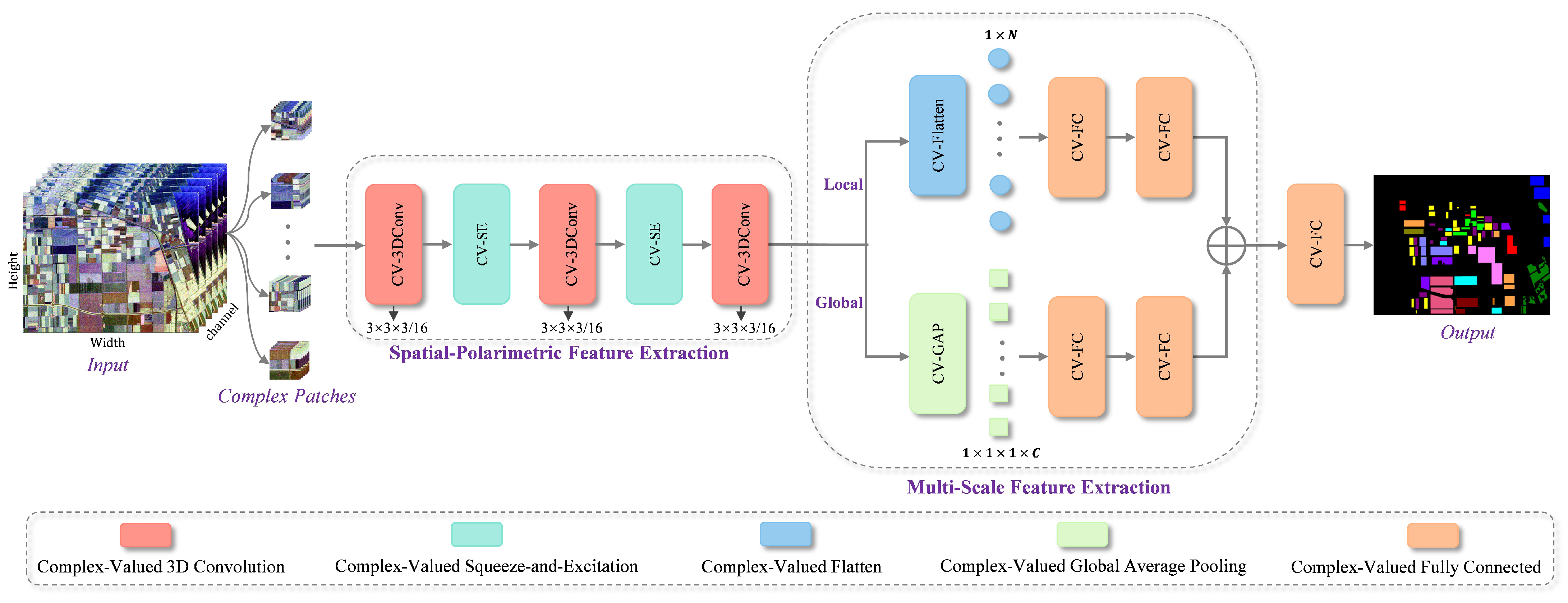
This paper introduces multi-scale feature extraction (MSFE), which utilizes a 3D complex-valued network for the classification of PolSAR images. Unlike the existing hybrid methods, this approach designs a multi-scale feature-extraction network based on CV-3DConv, and its parallel branch structure is used for modeling the multi-scale receptive field, capturing more discriminative features at different levels, which further enhances the classification performance of PolSAR images. The key contributions of this work are summarized as follows:

• Based on the characteristics of PolSAR images, a 3D complex-valued network combining CV-3DConv and complex-valued squeeze-and-excitation (CV-SE) is proposed, which effectively extracts spatial and polarimetric dimensions features that include both amplitude and phase information from PolSAR images, resulting in more representative and discriminative complex-valued features.
• Through the parallel branching structure, the multi-scale receptive field modeling of global and local features is realized. Global features are used to extract the overall semantic information of the image, while local features effectively guide the network in capturing regional semantic information, thus effectively balancing global and local spatial consistency.
• Our experimental results show that MSFE demonstrates significant advantages in both classification accuracy and robustness.

The paper is structured as follows: Section 2 introduces the MSFE method; Section 3 presents and analyzes comparative experimental results on three PolSAR images; Section 4 provides ablation studies and an analysis of the model’s generalization capability; and Section 5 concludes this work.

2. Method

In this section, we provide a detailed description of the overall structure of MSFE and its individual components. Specifically, multi-scale feature modeling plays a key role in multi-instance problems, enabling MSFE to more effectively learn and understand the complex characteristics of PolSAR data, thereby improving performance in PolSAR image classification tasks.

2.1. Network Architecture

Unlike traditional classification tasks, PolSAR image classification is a dense prediction task with semantic segmentation characteristics. Each training sample contains one or more instances, but the label only provides category information. Specifically, let the training set of a PolSAR image be denoted as S, where each sample $S_i$ consists of multiple instances $x_1,x_2,\dots ,x_m(m\in \mathbb{N})$, and the label $y_i$ indicates the sample’s category. Existing PolSAR image classification networks do not fully account for this characteristic. They focus on local image details while neglecting global context, limiting performance in such tasks. Inspired by the DenseCL [46] approach and the characteristics of PolSAR complex-valued data, we propose the MSFE method, as depicted in Figure 1.

The MSFE framework primarily consists of a spatial–polarimetric feature-extraction module and a multi-scale feature-extraction module, aiming to effectively extract multi-scale features containing phase information for high-precision classification of PolSAR images. Specifically, MSFE first employs the spatial–polarimetric feature-extraction module to simultaneously extract complex-valued features along both the spatial and polarimetric dimensions. This process involves enhancing the richness of feature representation, using CV-3DConv, while improving the discriminability of the feature representation through CV-SE. Subsequently, the multi-scale feature-extraction module, with its parallel branch structure, models both the global and local features of the complex-valued input. The global features capture the overall structure and global semantic information of the image, while the local features guide the network to focus on regional structures and local semantic information. Finally, the multi-scale complex-valued features are fused at predetermined ratios, utilizing a multi-scale learning strategy that complements the advantages of different features, enabling the network to fully exploit the amplitude and phase information in the PolSAR images and achieve accurate classification.

2.1.1. Complex-Valued 3D Convolution

Convolution operations rely on the relationships between adjacent pixels to enhance the network’s ability to capture spatially correlated features. Unfortunately, traditional 2DConv processes each channel independently and cannot effectively extract correlations between polarimetric information in PolSAR images (illustrated in the 2DConv of Figure 2).

In contrast, 3DConv computes across all channels simultaneously (illustrated in the 3DConv of Figure 2), enabling the extraction of both spatial and polarimetric features, which significantly improves the model’s feature representation. In 3DConv, the input image X (with dimensions $Height\times Width\times Depth$) is convolved with a 3D kernel, and the results are summed. A scalar bias b is then added to produce the net output of the convolution layer. The mathematical expression is

$$Y_{(x,y,z)}=\sum _{i=1}^h\sum _{j=1}^w\sum _{k=1}^d{K}_{(i,j,k)}{X}_{(x+i,y+j,z+k)}+b,$$

(1)

where K denotes a 3DConv kernel of size $h\times w\times d$. After applying a nonlinear activation function $\sigma$ to (1), the output of the 3DConv layer is given by

$$Output\left(X\right)=\sigma \left(Y_{(x,y,z)}\right).$$

(2)

Although 3DConv outperforms 2DConv, in terms of feature-extraction capability, real-valued convolution cannot simultaneously learn amplitude and phase information, preventing the complex characteristics of PolSAR images from effectively supporting the classification task. To fully utilize the phase information in PolSAR data, we introduce the CV-3DConv, where the image data input for the convolution operation includes both real and imaginary components. As shown in Figure 2, for an input image $X=Re\left(X\right)+iIm\left(X\right)$ and convolution kernel $K=Re\left(K\right)+iIm\left(K\right)$, the output Y of the complex-valued convolution is

$$\begin{array}{cc}\hfill Y& =Re\left(Y\right)+iIm\left(Y\right)=X\ast K=\left(Re\right(X)+iIm(X\left)\right)\ast \left(Re\right(K)+iIm(K\left)\right)\hfill \\ \hfill & =Re\left(X\right)\ast Re\left(K\right)-Im\left(X\right)\ast Im\left(K\right)+i\left(Re\right(X)\ast Im(K)+Re(K)\ast Im(X\left)\right),\hfill \end{array}$$

(3)

where $Re(·)$ and $Im(·)$ denote the real and imaginary parts of the complex-valued convolution, and where i is the imaginary unit.

2.1.2. Complex-Valued Squeeze-and-Excitation

In PolSAR image classification, the network is required to process multiple scattering channels from the central and neighboring pixels. The SE mechanism enhances the network’s ability to model key information by adaptively recalibrating channel-wise feature responses, improving feature discriminability and overall performance. Specifically, by integrating the SE attention mechanism, the network can automatically identify critical channel features within the input data and assign higher importance to them, while suppressing redundant or task-irrelevant information. This attention mechanism effectively captures inter-channel dependencies with negligible additional computational overhead, leading to improved network performance and generalization ability.

Figure 3 is the structure of the CV-SE module. In this module, a complex-valued convolutional transformation $F_{tr}$ maps the complex-valued input X into a feature map $u_c\in {\mathbb{C}}^{H\times W\times D\times C}$, where $u_c$ represents the c-th $H\times W\times D$ matrix in u, and where C denotes the total number of channels.

During the squeeze stage $F_{sq}(·)$, complex-valued global average pooling (CV-GAP) compresses the $H\times W\times D\times C$ feature map into a $1\times 1\times 1\times C$ representation. The squeeze function is

$$z_c=F_{sq}\left(u_c\right)={\displaystyle \frac{1}{H\times W\times D}}\sum _{i=1}^H\sum _{j=1}^W\sum _{n=1}^D{u}_c(i,j,n).$$

(4)

As shown in the equation above, the input is compressed into a column vector of length C, each element representing the aggregated information of a specific channel. Next, in the excitation stage, a pair of complex-valued fully connected (CV-FC) layers is employed to model the importance of each channel, enabling the recalibration of feature responses according to their relevance to the task. This process enhances task-relevant features and suppresses irrelevant ones. The excitation function is formulated as

$$s=F_{ex}(z,W)=\sigma \left(g(z,W)\right)=\sigma \left(W_2\mathbb{C}ReLU\left(W_{1}z\right)\right),$$

(5)

where $\sigma$ denotes the Sigmoid activation function, and $W_1\in {\mathbb{R}}^{{\displaystyle \frac{C}{r}}\times C}$ and $W_2\in {\mathbb{R}}^{C\times {\displaystyle \frac{C}{r}}}$ are the weight matrices of the two CV-FC layers responsible for dimensionality reduction and expansion, respectively. Here, r is a reduction ratio, z is the output from the preceding squeeze layer. The final output $s\in [0,1]$, obtained after the Sigmoid activation, serves as the attention vector used to re-weight each channel of u, thereby enabling channel-wise feature recalibration.

2.2. Multi-Scale Feature Extraction

As shown in Figure 1, the multi-scale feature-extraction module is implemented through a parallel structure consisting of global and local feature branches. Both branches share the same input, but independently perform feature learning. Specifically, the global feature-extraction branch uses a GAP operation to pool the complex-valued input features, extracting global context information. This branch fully leverages the image-level global representation to capture the overall structure and global semantic information of the image, thereby enhancing the macro-level perception ability in PolSAR image classification tasks. In contrast, the local feature branch flattens the complex-valued input features through a flatten operation, ensuring the spatial consistency of the local representation. This enables the flexible capture of regional structures and local semantic information within the image. To effectively balance global and local features and maximize their complementary advantages, we perform weighted fusion of global and local features at a ratio of 30% and 70%. The validation of the optimal weight ratio is discussed in detail in Section 4.3. This multi-scale learning strategy not only ensures the spatial consistency of local representations but also considers the global consistency of the image, overcoming the limitations of traditional dense prediction tasks in handling either global or local information. It effectively enhances the feature prediction ability of the network in complex data, thereby improving the accuracy and robustness of PolSAR image classification tasks.

2.3. Loss Function

We learn from the weighted fused multi-scale features and optimize the feature expression by computing the cross-entropy loss between predicted outputs and actual class labels. Initially, a softmax classifier computes the probability distribution over categories for the input training data, as given by the following formula:

$${\widehat{y}}_l^m=Softmax\left(\right|X_{out}\left|\right),$$

(6)

here, $X_{out}$ is the output of the final CV-FC layer, making $X_{out}$ complex-valued. The $|·|$ denotes the modulus operation, so ${\widehat{y}}_l^m$ is real-valued. Next, the cross-entropy loss is employed to quantify the divergence between ground-truth labels and the predicted probabilities, as follows:

$$Loss=-\sum _{m=1}^M\sum _{l=1}^L{y}_l^{m}log\left({\widehat{y}}_l^m\right),$$

(7)

where L and M are the total quantity of classes and the total samples in the batch, and $y_l^m$ and ${\widehat{y}}_l^m$ represent the true and predicted labels, respectively.

2.4. PolSAR Data Pre-Processing

Constructing polarimetric feature vectors is crucial for PolSAR image classification. PolSAR images are captured by transmitting and receiving electromagnetic waves in various polarization modes, including both horizontal and vertical polarization. Each pixel in a PolSAR image is represented by a $2\times 2$ scattering matrix S, mathematically expressed as follows:

$$S=\left[\begin{array}{cc}{S}_{HH}& S_{HV}\\ S_{VH}& S_{VV}\end{array}\right],$$

(8)

The above expression records the scattering echo information of the terrain under any polarization state, including both amplitude and phase information. In this matrix, $S_{HH}$ and $S_{VV}$ are the co-polarization components, where the polarization modes of transmission and reception are the same; $S_{HV}$ and $S_{VH}$ are the cross-polarization components, where the polarization modes differ. The polarization coherence matrix T is a complex-conjugate symmetric matrix, with real diagonal elements. According to the reciprocity theorem ($S_{HV}=S_{VH}$), the polarization scattering matrix can be converted into T using the Pauli decomposition method:

$$T=\left[\begin{array}{ccc}{T}_{11}& T_{12}& T_{13}\\ T_{21}& T_{22}& T_{23}\\ T_{31}& T_{32}& T_{33}\end{array}\right],$$

(9)

where

$$\begin{array}{cc}\hfill T_{11}& ={\displaystyle \frac{1}{2}}{|S_{HH}+S_{VV}|}^2,\hfill \\ \hfill T_{12}& ={\displaystyle \frac{1}{2}}(S_{HH}+S_{VV}){(S_{HH}-S_{VV})}^{\ast },\hfill \\ \hfill T_{13}& =(S_{HH}+S_{VV})S_{HV}^{\ast },\hfill \\ \hfill T_{21}& ={\displaystyle \frac{1}{2}}{(S_{HH}+S_{VV})}^{\ast }(S_{HH}-S_{VV}),\hfill \\ \hfill T_{22}& ={\displaystyle \frac{1}{2}}{|S_{HH}-S_{VV}|}^2,\hfill \\ \hfill T_{23}& =(S_{HH}-S_{VV})S_{HV}^{\ast },\hfill \\ \hfill T_{31}& ={(S_{HH}+S_{VV})}^{\ast }{S}_{HV},\hfill \\ \hfill T_{32}& ={(S_{HH}-S_{VV})}^{\ast }{S}_{HV},\hfill \\ \hfill T_{33}& =2|S_{HV}{|}^2.\hfill \end{array}$$

(10)

In PolSAR image classification, a six-dimensional feature vector derived from the T is commonly used to represent the PolSAR image features. This feature vector can be expressed as

$$\begin{array}{c}\hfill T^{\prime }=[T_{11},T_{12},T_{13},T_{22},T_{23},T_{33}].\end{array}$$

(11)

3. Experiments

3.1. Settings and Datasets

The MSFE method is refined through the application of the Adam optimizer, with key hyperparameters configured as follows: a learning rate of 0.001, a batch size of 64, and 100 training epochs. Each pixel in the PolSAR image is defined using a $13\times 13$ sliding window, which helps to create a dataset compatible with the network’s input format. For network training, a random selection of 0.2% from the available labeled dataset is employed. All the experimental procedures are executed on a computational setup featuring a 12th Gen Intel(R) Core(TM) processor with 32GB of RAM, utilizing Python 3.9 and TensorFlow 2.10.0.

We validated the effectiveness of the proposed method using three PolSAR images focused on crop types. Figure 4, Figure 5 and Figure 6 show the Pauli RGB images and their corresponding ground truth label maps, while

Table 1. Statistics of categories, number, and proportion of each category in each dataset.

Flevoland-1989 Dataset			Flevoland-1991 Dataset			Indian Head Dataset
Class	Number	Proportion	Class	Number	Proportion	Class	Number	Proportion
Stem Beans	6103	3.78%	Potato	21,613	15.97%	Canola	459,096	22.28%
Peas	9111	5.71%	Fruit	4352	3.22%	Pea	255,108	12.38%
Rapeseed	14,944	8.27%	Oats	1394	1.03%	Flex	131,296	6.37%
Beet	9477	5.98%	Beet	10,817	7.99%	Lentil	217,186	10.54%
Forest	17,283	10.76%	Barley	24,543	18.13%	Spring Wheat	904,386	43.91%
Lucerne	10,050	6.07%	Onions	2130	1.57%	Hayfield	93,134	4.52%
Wheat 1	15,292	9.77%	Wheat	26,277	19.41%	-	-	-
Bare Soil	3078	3.05%	Beans	1082	0.80%	-	-	-
Grass	6269	4.21%	Peas	2160	1.60%	-	-	-
Water	12,690	7.89%	Maize	1290	0.95%	-	-	-
Barley	7156	4.53%	Flax	4310	3.18%	-	-	-
Wheat 2	10,591	6.65%	Rapeseed	28,235	20.86%	-	-	-
Wheat 3	21,300	13.26%	Grass	4204	3.11%	-	-	-
Potatoes	13,476	9.63%	Lucerne	2952	2.18%	-	-	-
Buildings	476	0.44%	-	-	-	-	-	-
Total	157,296	100%	Total	135,359	100%	Total	2,060,206	100%

provides a detailed breakdown of the categories, quantities, and proportions for each dataset. The descriptions of the individual datasets are as follows.

Flevoland-1989 dataset: this dataset consists of L-band fully polarized airborne SAR data released by NASA/JPL Laboratory, collected in 1989. The study area is in the Flevoland region of the Netherlands. The image size is $750\times 1024$. It includes 15 land cover categories. This dataset is widely used for validating PolSAR image classification methods.

Flevoland-1991 dataset: this dataset, also from L-band fully polarimetric airborne SAR data released by NASA/JPL Laboratory, was collected in 1991. The image size is $1020\times 1024$. It includes 14 land cover categories.

Indian Head dataset: this dataset, provided by the European Space Agency, was collected in 2009. It is based on Radarsat-2 satellite system data and simulated C-band fully polarized spaceborne SAR data according to Sentinel-1 satellite system parameters. The study area is at Indian Head Farm in Saskatchewan, Canada, with an image size of $1994\times 1697$. The dataset includes six land cover categories.

3.2. Evaluation Metrics

To thoroughly assess the classification capabilities of the various approaches, we conducted a pixel-by-pixel comparison between the full image classification results predicted by each method and the corresponding ground truth label map. Using the confusion matrix as a basis, this study adopted three well-established quantitative metrics: Overall Accuracy (OA), Average Accuracy (AA), and the Kappa Coefficient (Kappa) to systematically calculate and analyze the experimental results. Elevated metric values reflect better classification performance for the respective method in the context of PolSAR imagery.

These evaluation metrics offer a broad assessment of method performance from several perspectives. In the quantitative evaluation of PolSAR image classification, the confusion matrix serves as a core quantitative visualization tool and the basis for calculating OA, AA, and Kappa. It is mainly used to identify discrepancies between classification results and actual predictions. We denote the confusion matrix as $\mathrm{M}\in {\mathbb{R}}^{K\times K}$, where K is the total quantity of categories in the test set. Its columns represent the predicted categories, with each column’s sum indicating the number predicted for that category. The rows correspond to the actual categories of the samples, with each row sum reflecting the actual number for that category. The diagonal elements indicate the number of correct predictions for each category, while the off-diagonal elements represent the number of incorrect predictions.

OA is defined as the ratio of correct predictions to the total quantity of test samples, applying equal weight to each test sample and reflecting the probability that the classifier’s predicted results align with the ground truth labels. OA is defined as follows, based on the confusion matrix:

$$\begin{array}{c}\hfill OA={\displaystyle \frac{{\sum }_{i=1}^{K}M(i,i)}{{\sum }_{i=1}^K{\sum }_{j=1}^{K}M(i,j)}}.\end{array}$$

(12)

AA is the average accuracy across each predicted category, where the accuracy for each category is the ratio of correct predictions to the actual number for that category. Its mathematical expression is

$$\begin{array}{c}\hfill AA={\displaystyle \frac{1}{K}}\sum _{i=1}^K{\displaystyle \frac{M(i,i)}{{\sum }_{j=1}^{K}M(i,j)}}.\end{array}$$

(13)

Kappa is a commonly used metric in statistics for measuring consistency, accounting for the imbalance in data categories and providing a more comprehensive assessment of classification performance. Its mathematical expression is

$$\begin{array}{c}\hfill Kappa={\displaystyle \frac{OA-p_e}{1-p_e}},\end{array}$$

(14)

where

$$\begin{array}{c}\hfill p_e={\displaystyle \frac{{\sum }_{i=1}^K\left({\sum }_{j=1}^{K}M(i,j){\sum }_{j=1}^{K}M(j,i)\right)}{{\left({\sum }_{i=1}^K{\sum }_{j=1}^{K}M(i,j)\right)}^2}}.\end{array}$$

(15)

3.3. Comparison with Existing Works

We employed both quantitative measures and qualitative visualizations to thoroughly assess the effectiveness of the proposed MSFE method. We compared the MSFE method with five representative deep learning methods, including real-valued 2D and 3D networks and complex-valued 2D and 3D networks [19,26,28,44]. The real-valued networks used $\left[\right|T_{11}|,|T_{12}|,|T_{13}|,|T_{22}|,|T_{23}|,|T_{33}\left|\right]$ as input features, while the complex-valued networks used the complex form of the polarization coherence matrix $[T_{11},T_{12},T_{13},T_{22},T_{23},T_{33}]$, fully exploiting phase information. To ensure fairness, all the compared methods were implemented using open-source code or built on existing open-source implementations.

3.3.1. Flevoland-1989 Dataset

Table 2. Quantitative results of MSFE and different methods on the Flevoland-1989 dataset. The best performance is highlighted in bold.

Class	RV-CNN	3D-CNN	CV-CNN	HybridCVNet	SDF2Net	MSFE
Stem Beans	81.70%	79.35%	85.14%	93.68%	87.97%	97.92%
Peas	83.66%	89.45%	89.29%	92.13%	94.22%	95.06%
Rapeseed	75.38%	97.48%	83.64%	88.26%	73.98%	96.94%
Beet	72.38%	96.15%	60.27%	96.10%	96.90%	91.62%
Forest	77.64%	94.26%	77.43%	93.40%	95.52%	95.68%
Lucerne	71.32%	91.08%	74.27%	91.55%	84.89%	91.05%
Wheat 1	67.13%	92.73%	65.58%	98.18%	97.35%	98.68%
Bare Soil	0.45%	45.52%	0.42%	35.80%	98.83%	97.11%
Grass	37.26%	54.79%	20.00%	87.65%	86.82%	87.81%
Water	50.32%	63.87%	54.19%	63.73%	69.60%	66.80%
Barley	73.71%	84.87%	80.55%	92.72%	82.80%	89.77%
Wheat 2	81.67%	92.28%	71.29%	95.80%	89.59%	91.48%
Wheat 3	90.06%	96.81%	95.10%	98.55%	98.96%	99.18%
Potatoes	95.35%	79.21%	97.28%	97.57%	98.76%	99.95%
Buildings	43.49%	99.58%	14.29%	73.11%	97.90%	79.62%
OA	74.05%	87.00%	74.58%	90.73%	90.09%	93.23%
AA	66.77%	83.83%	64.58%	86.55%	90.27%	91.91%
Kappa	71.63%	85.81%	72.17%	89.88%	89.18%	92.60%

lists the quantitative results of all the comparison methods. In supervised learning, network performance is often limited by the number of labeled samples. Therefore, for the simpler 2D convolution networks (such as RV-CNN and CV-CNN), the OA was below 80%. Among these, the CV-CNN considered the PolSAR data characteristics and phase information, resulting in better evaluation metrics compared to the RV-CNN. Note that 3DConv enhances feature learning ability by adding a depth dimension, enabling the network to extract more advanced semantic features when processing complex data. Consequently, both the real-valued network 3D-CNN and the complex-valued networks SDF2Net and HybridCVNet achieved an average improvement of approximately 14.96%, 21.21%, and 16.39%, respectively, in the OA, AA, and Kappa metrics, compared to the 2D convolution network. These significant improvements in metrics further validate the advantage of 3DConv in learning both spatial and polarimetric dimensional features simultaneously. Compared to 3D-CNN, the complex-valued networks HybridCVNet and SDF2Net, which can learn phase information, showed stronger advantages in PolSAR image classification tasks (with OA exceeding 90%). Specifically, the HybridCVNet method based on the ViT achieved OA, AA, and Kappa of 90.73%, 86.55%, and 89.88%, respectively. The structural design of the 3D complex-valued network MSFE successfully integrated global features and performed weighted fusion with local features, resulting in excellent performance across multiple classes.

However, this joint feature learning strategy inevitably introduces feature coupling during network training. This issue is particularly pronounced for categories with single scattering characteristics, ambiguous boundaries, or highly uneven spatial scale distributions. Under such conditions, multi-scale feature fusion may fail to generate sufficiently discriminative representations, leading to a decline in classification accuracy for specific classes. For example, Beet is characterized primarily by volume scattering and features a compact planting structure with limited texture variation. Local features thus offer limited discriminatory power, while global features may incorporate background information from surrounding categories, compromising classification robustness. Bare Soil, dominated by surface scattering, presents substantial small-scale heterogeneity, due to variations in tillage intensity, soil moisture, and surface roughness. Consequently, local features may capture inconsistent information, and global features often lack stable structural patterns, resulting in weak overall feature representation. Water exhibits specular reflection with low backscattering coefficients. Although it typically shows spatial continuity, boundary regions (e.g., water–land interfaces) are frequently affected by waves, aquatic vegetation, or sediment, introducing instability in edge features and degrading discriminability.

Overall, MSFE achieved the highest classification performance, with improvements of 2.50%, 5.36%, and 2.72% in OA, AA, and Kappa, respectively, compared to the state-of-the-art HybridCVNet method. These experimental results thoroughly demonstrate that even with extremely scarce labeled samples (0.2%), the proposed method still exhibits outstanding performance in PolSAR image classification tasks involving multi-instance problems, thus advancing the practical application of supervised learning methods in PolSAR image classification.

Figure 7 shows the qualitative visual classification results. The 2DConv method struggled to effectively learn the correlations between polarization channels, resulting in relatively poor classification performance (Figure 7a,c). In contrast, the 3D networks based on 3DConv (Figure 7b,d–f) benefited from processing all polarization channels simultaneously, producing clearer results with more defined boundaries and better spatial continuity. These networks showed significant improvements in misclassification for categories such as Bare Soil, Rapeseed, and Wheat 2. More importantly, Figure 7d–f learned both amplitude and phase information from PolSAR images, leading to superior overall performance compared to Figure 7b. Despite the relatively good results from the 3D complex-valued network, some issues remain. Specifically, in Figure 7d a large portion of Bare Soil is misclassified as Potatoes (highlighted by the yellow rectangle), and in Figure 7e some Rapeseed is misclassified as Wheat 2 (highlighted by the white rectangle). In contrast, the method shown in Figure 7f, with its multi-scale feature modeling capability, better aligns with the ground truth labels, demonstrating the stronger representational power and discriminative ability of the features learned by MSFE.

3.3.2. Flevoland-1991 Dataset

Table 3. Quantitative results of MSFE and different methods on the Flevoland-1991 dataset. The best performance is highlighted in bold.

Class	RV-CNN	3D-CNN	CV-CNN	HybridCVNet	SDF2Net	MSFE
Potato	85.07%	99.20%	88.91%	99.10%	99.63%	99.51%
Fruit	84.60%	99.40%	81.23%	88.83%	49.13%	85.43%
Oats	61.26%	44.62%	77.26%	82.14%	72.02%	95.27%
Beet	64.90%	89.94%	79.92%	96.75%	99.27%	96.63%
Barley	64.96%	73.86%	85.92%	90.84%	99.08%	99.50%
Onions	19.06%	7.32%	17.32%	25.87%	6.71%	23.15%
Wheat	79.05%	95.79%	89.46%	99.16%	99.86%	99.89%
Beans	11.09%	2.59%	3.97%	0%	1.76%	81.79%
Peas	89.54%	100%	66.67%	95.83%	100%	96.71%
Maize	51.55%	69.84%	46.51%	0%	0%	52.95%
Flax	36.69%	85.33%	76.89%	55.75%	100%	99.91%
Rapeseed	80.85%	91.67%	87.57%	95.54%	92.60%	99.34%
Grass	61.56%	76.24%	63.27%	50.07%	69.58%	71.10%
Lucerne	69.88%	81.78%	66.33%	89.33%	74.53%	82.32%
OA	73.03%	87.06%	82.88%	90.12%	91.51%	95.74%
AA	61.43%	72.68%	66.52%	69.23%	68.87%	84.54%
Kappa	68.23%	84.72%	79.77%	88.40%	89.98%	94.98%

presents the quantitative results of all the comparison methods. Overall, the classification performance of CV-CNN, RV-CNN, and 3D-CNN was generally lower than that of the 3D complex-valued network. The methods combining feature fusion from the three-branch architecture, such as SDF2Net and the HybridCVNet of incorporation ViT, exhibited relatively prominent performance, with OA exceeding 90% and Kappa close to 90%. However, these methods showed lower AA values of 68.87% and 69.23%, respectively, with particularly low accuracies in the Beans and Maize categories. This indicates that the aforementioned methods fail to provide stable classification results when handling certain complex or data-scarce categories. In contrast, MSFE showed superior performance in categories like Oats, Barley, Wheat, and Rapeseed, maintaining high classification accuracy even for categories where other methods were unstable. For instance, the accuracy for Beans reached 81.79%, which was significantly higher than that of the other methods. Compared to the second-best SDF2Net, MSFE improved OA, AA, and Kappa by 4.23%, 15.67%, and 5.00%, respectively. This further validates the effectiveness of the MSFE method in PolSAR image classification tasks with scarce labeled samples, proving that it can significantly improve classification performance under conditions of limited samples and complex categories.

Figure 8 displays the qualitative visual classification results of different methods. A comparison reveals severe confusion between categories such as Wheat, Lucerne, and Oats. Specifically, Lucerne and Oats are misclassified as Wheat in Figure 8a,c, while in Figure 8b,d,e, they are incorrectly classified as Barley, Grass, or Potato (highlighted by the white rectangle). Further observation reveals that most of the methods faced considerable difficulties in classifying Beans, with a majority misclassifying them as Beet, Onions, or Barley, especially in Figure 8d, where Beans are almost entirely misclassified as Beet (highlighted by the yellow rectangle). However, in Figure 8f these misclassifications or confusions are significantly improved, particularly in the classification of Beans, showing a much higher accuracy. This indicates that MSFE, through multi-scale feature fusion, effectively expands the scale and richness of feature extraction, leading to more consistent classification results with ground truth labels. It further confirms that MSFE provides more accurate and robust classification results when handling complex PolSAR images.

3.3.3. Indian Head Dataset

Table 4. Quantitative results of MSFE and different methods on the Indian Head dataset. The best performance is highlighted in bold.

Class	RV-CNN	3D-CNN	CV-CNN	HybridCVNet	SDF2Net	MSFE
Canola	78.93%	89.14%	81.10%	89.72%	90.87%	90.16%
Pea	79.91%	82.60%	81.17%	86.07%	80.51%	86.66%
Flex	32.24%	34.91%	34.00%	52.94%	41.93%	37.80%
Lentil	72.13%	63.70%	73.35%	78.34%	68.60%	79.11%
Spring Wheat	85.65%	90.70%	84.91%	84.35%	91.33%	91.88%
Hayfield	47.14%	54.49%	47.99%	57.95%	51.06%	58.99%
OA	76.87%	81.31%	77.47%	81.93%	82.52%	84.57%
AA	66.00%	69.26%	67.09%	74.90%	70.71%	74.10%
Kappa	67.95%	73.89%	68.87%	75.44%	75.50%	78.51%

presents the quantitative results of all the comparison methods. The Indian Head dataset has a large image size, with labeled categories covering approximately 60% of the image. As a result, using only 0.2% of the labeled samples was sufficient to support the convergence of the supervised learning methods and ensure their robustness. The 3D network outperformed the 2D network in this dataset, confirming that 3DConv can fully leverage the complex relationships between spatial and polarimetric information, improving classification accuracy. HybridCVNet and SDF2Net achieved the best classification accuracy in the Canola and Flex categories, respectively, but MSFE excelled in multiple categories, particularly Pea (86.66%) and Spring Wheat (91.88%), demonstrating its superior performance. Additionally, MSFE achieved the highest values in all three evaluation metrics, improving OA, AA, and Kappa by 2.05%, 3.39%, and 3.01%, respectively, compared to the second-best method, SDF2Net.

Figure 9 presents the qualitative visualization of the classification results for the different methods. It can be seen that the dataset has a relatively large proportion of categories, with dense distribution, especially with the Spring Wheat category, which accounts for approximately half of the total categories. As a result, there were many misclassifications between categories, such as confusion between Flex and Lentil, Lentil and Canola, and Flex and Pea. However, overall, the classification results in Figure 9f show a significantly higher overlap with the ground truth labels, particularly in areas highlighted by white and red rectangles. This suggests that the MSFE method can effectively reduce misclassifications between categories, improve overall classification accuracy, and demonstrate strong stability and robustness, especially in cases with complex categories and dense samples.

4. Ablation Studies

We conducted a series of ablation studies using the Flevoland-1989 dataset to assess the impact of each module, the multi-scale feature weight, and the sampling rates on MSFE. We also compared network parameters with classification performance. Simultaneously, the non-agricultural Oberpfaffenhofen dataset was used to validate the generalizability of MSFE. All the experiments followed a uniform training scheme.

4.1. Module Contributions

To investigate the contributions of each MSFE component, we conducted a module ablation study, with the results in

Table 5. Quantitative results of the ablation study of the proposed MSFE. The best performance is highlighted in bold.

	CV-3DConv	CV-SE	Multi-Scale Feature	OA	AA	Kappa
Group 1	×	×	×	88.67%	82.75%	87.62%
Group 2	√	×	×	91.07%	89.61%	90.23%
Group 3	√	√	×	91.45%	91.13%	90.66%
Group 4	√	√	√	93.23%	91.91%	92.60%

, where ‘√’ indicates inclusion of the module in the experiment, while ‘×’ indicates it was not. Group 1 served as the baseline reference network, which was a 3D real-valued network without attention mechanisms or multi-scale features. Since CV-3DConv can simultaneously learn both the amplitude and the phase information of PolSAR data, replacing the 3DConv with CV-3DConv in Group 1 allowed the network to capture complex data structures more precisely. For example, compared to Group 1, Group 2 achieved improvements of 2.40%, 6.86%, and 2.61% in OA, AA, and Kappa, respectively, with a particularly significant improvement in AA. This demonstrates that the simultaneous learning of amplitude and phase information enables the network to provide stable classification performance across various categories. To enhance the interdependencies among complex-valued feature channels, the CV-SE module was introduced in Group 2, further improving the network’s performance. Considering the specific attributes of PolSAR image classification, a multi-scale feature-extraction strategy was designed to address the multi-instance problem, effectively modeling both global and local features and capturing key characteristics at the global image level and local region level. For instance, Group 4 showed improvements of 1.78%, 0.78%, and 1.94% in OA, AA, and Kappa, respectively, compared to Group 3. In summary, when all three modules were used together, the network achieved the best classification performance. Compared to the baseline reference network (Group 1), the classification performance of Group 4 was significantly improved (OA: +4.56%, AA: +9.16%, Kappa: +4.98%).

4.2. Number of Parameters Analysis

In CNN methods, the number of learnable parameters directly determines the complexity of the model. Generally, models with fewer parameters are more efficient, particularly in practical applications where computational resources are limited. Reducing the number of parameters can effectively lower both the training and inference time costs. Therefore, we compared the number of parameters across various methods, as shown in Figure 10.

Except for the proposed method, the number of parameters in 2D network methods (such as RV-CNN, CV-CNN) is significantly lower than in 3D network methods (such as 3D-CNN, SDF2Net, and HybridCVNet). However, 2D network methods, due to their relatively simple network structures, suffer from insufficient feature-extraction capabilities, resulting in lower classification accuracy that fails to meet practical application demands. In contrast, while 3D networks generally achieve higher classification accuracy, they often rely on 3DConv modules to enhance feature-extraction capacity, which significantly increases the number of parameters. In particular, HybridCVNet incorporates additional ViT components, resulting in even greater memory consumption and computational cost. Consequently, traditional supervised learning methods have not achieved an effective balance between classification accuracy and computational efficiency, limiting their practical deployment in resource-constrained environments. In this paper, MSFE achieves superior classification accuracy with substantially fewer parameters, establishing a new “Pareto front” in the two-dimensional space of “model complexity and classification performance.” This outcome confirms the effectiveness of the multi-scale learning strategy in preserving local spatial consistency and capturing global semantic information without the need for excessively complex architectures. Consequently, MSFE offers a promising solution for deployment in embedded systems and edge computing scenarios where computational resources are limited, providing a balanced compromise between model efficiency and classification precision.

4.3. Multi-Scale Feature Weight

To determine the optimal ratio between global and local features, we conducted an experimental study on their weight distribution, with the results shown in

Table 6. Ablation study of multi-scale feature weight. The best performance is highlighted in bold.

Local Feature	Global Feature	OA	AA	Kappa
0	1	85.88%	80.91%	84.57%
0.1	0.9	91.30%	88.93%	90.50%
0.2	0.8	91.61%	90.74%	90.84%
0.3	0.7	91.70%	89.74%	90.94%
0.4	0.6	92.06%	87.45%	91.32%
0.5	0.5	92.27%	89.79%	91.56%
0.6	0.4	93.16%	91.77%	92.53%
0.7	0.3	93.23%	91.91%	92.60%
0.8	0.2	92.58%	91.42%	91.90%
0.9	0.1	91.61%	90.61%	90.84%
1	0	90.28%	89.70%	89.38%

. As the global feature weight increased from 0 to 0.3, OA improved by 2.95%, AA increased by 2.21%, and Kappa rose by 3.22%. However, as the global feature weight continued to increase, all the evaluation metrics declined rapidly. Additionally, Figure 11 shows the effect of changes in local feature weight on classification accuracy. The results indicate that as the weight of the local features increased, OA, AA, and Kappa followed an overall trend of first increasing and then decreasing. Notably, when the local feature weight ranged from 0.3 to 0.5, AA exhibited an abnormal decline, which was mainly attributed to the intensified coupling effect between global and local features as their weights approached parity, thereby affecting the discrimination of certain categories. Overall, when the local feature weight was set to 0.7, all three evaluation metrics reached their maximum values, further validating the effectiveness of the multi-scale features designed for multi-instance problems. Therefore, in this study the weights of the global and local features were set to 0.3 and 0.7, respectively.

4.4. Sampling Rates

To further evaluate the robustness of the MSFE, we performed a sensitivity analysis using label samples with different sampling ratios. As shown in

Table 7. Parameter analysis of sampling rates. The best performance is highlighted in bold.

Sampling Rates	Model	OA	AA	Kappa
0.1%	RV-CNN	66.18%	60.03%	63.14%
	3D-CNN	81.44%	76.37%	79.72%
	CV-CNN	72.32%	64.10%	69.76%
	HybridCVNet	85.57%	83.27%	84.25%
	SDF2Net	85.16%	74.81%	83.77%
	MSFE	86.40%	79.39%	85.13%
0.2%	RV-CNN	73.54%	64.80%	71.01%
	3D-CNN	88.24%	83.67%	87.15%
	CV-CNN	74.58%	64.58%	72.17%
	HybridCVNet	88.50%	84.37%	87.44%
	SDF2Net	90.09%	90.27%	89.18%
	MSFE	93.23%	91.91%	92.60%
0.4%	RV-CNN	77.50%	70.04%	75.38%
	3D-CNN	92.75%	89.60%	92.08%
	CV-CNN	80.24%	75.01%	78.45%
	HybridCVNet	93.29%	90.83%	92.68%
	SDF2Net	94.33%	92.89%	93.81%
	MSFE	96.27%	95.47%	95.92%
0.8%	RV-CNN	78.80%	75.62%	76.88%
	3D-CNN	94.63%	93.64%	94.14%
	CV-CNN	82.93%	78.85%	81.38%
	HybridCVNet	95.57%	95.74%	95.17%
	SDF2Net	95.25%	95.10%	94.82%
	MSFE	97.50%	96.77%	97.27%
1.0%	RV-CNN	80.02%	75.46%	78.22%
	3D-CNN	95.45%	94.77%	95.03%
	CV-CNN	81.20%	77.93%	79.50%
	HybridCVNet	97.75%	96.62%	97.54%
	SDF2Net	97.42%	97.17%	97.19%
	MSFE	98.06%	97.38%	97.89%

, increasing the sampling rate improved the accuracy of all the methods. Nonetheless, the performance of the 2D network consistently lagged behind that of the 3D network. When the sampling rate reached or exceeded 0.4%, the OA of all the 3D networks exceeded 90%, validating the advantage of 3DConv in PolSAR image classification. The introduction of phase information allowed HybridCVNet and SDF2Net to outperform the 3D-CNN. The ViT-based method required more training samples to converge than the CNN-based method. Therefore, when the sampling rate reached 0.8%, HybridCVNet’s performance began to surpass that of SDF2Net. Notably, regardless of the sampling rate, MSFE consistently outperformed the other networks.

4.5. Generalization Study

The Oberpfaffenhofen dataset was acquired using L-band E-SAR in the Oberpfaffenhofen region of Germany in 2002, with an image size of $1300\times 1200$. It includes three land cover categories with the following proportions: Built-up Areas (25.01%), Wood Land (18.81%), and Open Areas (56.18%), as shown in Figure 12a,b.

As shown in Figure 12b, most pixels in the Oberpfaffenhofen dataset are classified into well-defined land cover categories. Although the training samples were selected from a small proportion of the labeled data, the dataset size was sufficient for effective training of the supervised models. As a result, the performance differences among the methods in

Table 8. Quantitative results of MSFE and different methods on the Oberpfaffenhofen dataset. The best performance is highlighted in bold.

Class	RV-CNN	3D-CNN	CV-CNN	HybridCVNet	SDF2Net	MSFE
Built-up Areas	83.22%	88.16%	82.65%	86.24%	86.24%	88.34%
Wood Land	85.43%	92.51%	87.25%	97.49%	95.08%	92.72%
Open Areas	93.27%	96.46%	93.46%	95.45%	96.36%	96.86%
OA	89.28%	93.64%	89.59%	93.53%	93.59%	93.95%
AA	87.31%	92.38%	87.79%	93.06%	92.56%	92.64%
Kappa	81.79%	89.13%	82.28%	89.06%	89.07%	89.66%

are minimal. Both RV-CNN and CV-CNN achieved OA near 90%. The networks based on 3DConv consistently outperformed those using 2DConv, highlighting the advantage of 3DConv in capturing complex spatial–polarimetric correlations in PolSAR imagery. This capability enabled better utilization of the data’s intrinsic structure, leading to improved classification performance. Notably, the proposed MSFE method demonstrated strong discriminative power across categories, achieving the highest OA (93.95%) and Kappa coefficient (89.66%).

The visual results in Figure 13 confirm that the category distributions were compact and that the classification performance across different methods aligns with the quantitative analysis in Table 8. However, MSFE resulted in fewer misclassifications, particularly in distinguishing Built-up Areas from Wood Land and Open Areas from Built-up Areas, as highlighted by the white rectangles in Figure 13. This indicates that MSFE demonstrates superior classification consistency.

5. Conclusions

In this paper, we propose a PolSAR image classification method called MSFE. The method is based on a 3D complex-valued network framework, which effectively captures both spatial and polarimetric features, incorporating amplitude and phase information from PolSAR images. Additionally, by integrating global and local features, the method establishes a learning strategy with a multi-scale receptive field, ensuring the learning of regional structures and local semantic information while also incorporating global structure and global semantic information. Our experimental results show that MSFE has strong feature-extraction capabilities and multi-scale feature modeling ability, significantly improving classification accuracy. Future work will focus on extracting more discriminative features to better address the multi-instance problem in dense prediction tasks.

References

1. Shang, R.H.; Wang, J.M.; Jiao, L.C.; Yang, X.H.; Li, Y.Y. Spatial feature-based convolutional neural network for PolSAR image classification. Appl. Soft. Comput. 2022, 123, 108922. [Google Scholar] [CrossRef]
2. Silva-Perez, C.; Marino, A.; Lopez-Sanchez, J.M.; Cameron, I. Multitemporal polarimetric SAR change detection for crop monitoring and crop type classification. IEEE J. Sel. Top. Appl. Earth Obs. Remote Sens. 2021, 14, 12361–12374. [Google Scholar] [CrossRef]
3. Datcu, M.; Huang, Z.; Anghel, A.; Zhao, J.; Cacoveanu, R. Explainable, physics-aware, trustworthy artificial intelligence: A paradigm shift for synthetic aperture radar. IEEE Geosci. Remote Sens. Mag. 2023, 11, 8–25. [Google Scholar] [CrossRef]
4. Shi, H.T.; Zhao, L.L.; Yang, J.; Lopez-Sanchez, J.M.; Zhao, J.Q.; Sun, W.D.; Shi, L.; Li, P.X. Soil moisture retrieval over agricultural fields from L-band multi-incidence and multitemporal PolSAR observations using polarimetric decomposition techniques. Remote Sens. Environ. 2021, 261, 112485. [Google Scholar] [CrossRef]
5. Song, X.Y.; Zhang, L.; Lu, Z.; Wu, J.C.; Song, R.Q.; Liang, H.Y.; Bian, W.W. Toward retrieving discontinuous deformation of bridges by MTInSAR with adaptive segmentation. IEEE Trans. Geosci. Remote Sens. 2024, 62, 5202215. [Google Scholar] [CrossRef]
6. Zeng, Y.; Wang, D.; Tian, T.; Zhang, Y. Research advances on crop classification using PolSAR data. China Agric. Inform. 2020, 32, 13–26. [Google Scholar]
7. Yamaguchi, Y.; Moriyama, T.; Ishido, M.; Yamada, H. Four-component scattering model for polarimetric SAR image decomposition. IEEE Trans. Geosci. Remote Sens. 2005, 43, 1699–1706. [Google Scholar] [CrossRef]
8. Freeman, A.; van Zyl, J.J.; Klein, J.D.; Zebker, H.A.; Shen, Y. Calibration of stokes and scattering matrix format polarimetric SAR data. IEEE Trans. Geosci. Remote Sens. 1992, 30, 531–539. [Google Scholar] [CrossRef]
9. Cloude, S.R.; Pottier, E. An entropy based classification scheme for land applications of polarimetric SAR. IEEE Trans. Geosci. Remote Sens. 1997, 35, 68–78. [Google Scholar] [CrossRef]
10. Lee, J.S.; Grunes, M.R.; Ainsworth, T.L.; Du, L.J.; Schuler, D.L.; Cloude, S.R. Unsupervised classification using polarimetric decomposition and the complex Wishart classifier. IEEE Trans. Geosci. Remote Sens. 1999, 37, 2249–2258. [Google Scholar]
11. Lee, J.S.; Schuler, D.L.; Lang, R.H.; Ranson, K.J. K-distribution for multi-look processed polarimetric SAR imagery. In Proceedings of the IEEE International Geoscience and Remote Sensing Symposium (IGARSS), Pasadena, CA, USA, 8–12 August 1994; pp. 2179–2181. [Google Scholar]
12. Doulgeris, A.P.; Anfinsen, S.N.; Eltoft, T. Classification with a non-Gaussian model for PolSAR data. IEEE Trans. Geosci. Remote Sens. 2008, 46, 2999–3009. [Google Scholar] [CrossRef]
13. Lardeux, C. Support vector machine for multifrequency SAR polarimetric data classification. IEEE Trans. Geosci. Remote Sens. 2009, 47, 4143–4152. [Google Scholar] [CrossRef]
14. Masjedi, A.; Valadan Zoej, M.J.; Maghsoudi, Y. Classification of polarimetric SAR images based on modeling contextual information and using texture features. IEEE Trans. Geosci. Remote Sens. 2016, 54, 932–943. [Google Scholar] [CrossRef]
15. Bi, H.; Xu, L.; Cao, X.; Xue, Y.; Xu, Z. Polarimetric SAR image semantic segmentation with 3D discrete wavelet transform and Markov random field. IEEE Trans. Image Process. 2020, 29, 6601–6614. [Google Scholar] [CrossRef]
16. Kong, J.A.; Swartz, A.A.; Yueh, H.A.; Novak, L.M.; Shin, R.T. Identification of terrain cover using the optimum polarimetric classifier. J. Electromagn. Waves Appl. 1988, 2, 171–194. [Google Scholar]
17. Tao, M.; Zhou, F.; Liu, Y.; Zhang, Z. Tensorial independent component analysis-based feature extraction for polarimetric SAR data classification. IEEE Trans. Geosci. Remote Sens. 2015, 53, 2481–2495. [Google Scholar] [CrossRef]
18. Hua, W.Q.; Xie, W.; Jin, X.M. Three-channel convolutional neural network for polarimetric SAR images classification. IEEE J. Sel. Top. Appl. Earth Obs. Remote Sens. 2020, 13, 4895–4907. [Google Scholar] [CrossRef]
19. Zhou, Y.; Wang, H.; Xu, F.; Jin, Y.Q. Polarimetric SAR image classification using deep convolutional neural networks. IEEE Geosci. Remote Sens. Lett. 2016, 13, 1935–1939. [Google Scholar] [CrossRef]
20. Liu, G.Y.; Li, Y.Y.; Chen, Y.Q.; Shang, R.H.; Jiao, L.C. Pol-NAS: A neural architecture search method with feature selection for PolSAR image classification. IEEE J. Sel. Top. Appl. Earth Obs. Remote Sens. 2022, 15, 9339–9354. [Google Scholar] [CrossRef]
21. Zhang, W.T.; Liu, L.; Bai, Y.; Li, Y.B.; Guo, J. Crop classification based on multi-temporal PolSAR images with a single tensor network. Pattern Recognit. 2023, 143, 109773. [Google Scholar] [CrossRef]
22. Shang, R.H.; Hu, M.W.; Feng, J.; Zhang, W.T.; Xu, S.H. A lightweight PolSAR image classification algorithm based on multi-scale feature extraction and local spatial information perception. Appl. Soft. Comput. 2025, 170, 112676. [Google Scholar] [CrossRef]
23. Hua, W.Q.; Wang, Y.; Yang, S.J.; Jin, X.M. PolSAR image classification based on multi-modal contrastive fully convolutional network. Remote Sens. 2024, 16, 296. [Google Scholar] [CrossRef]
24. Barrachina, J.; Ren, C.; Vieillard, G.; Morisseau, C.; Ovarlez, J.P. Real-and complex-valued neural networks for SAR image segmentation through different polarimetric representations. In Proceedings of the IEEE International Conference on Image Processing (ICIP), Bordeaux, France, 16–19 October 2022; pp. 1456–1460. [Google Scholar]
25. Asiyabi, R.M.; Datcu, M.; Nies, H.; Anghel, A. Complex-valued vs. real-valued convolutional neural network for PolSAR data classification. In Proceedings of the IEEE International Geoscience and Remote Sensing Symposium (IGARSS), Kuala Lumpur, Malaysia, 17–22 July 2022; pp. 421–424. [Google Scholar]
26. Zhang, Z.; Wang, H.; Xu, F.; Jin, Y.Q. Complex-valued convolutional neural network and its application in polarimetric SAR image classification. IEEE Trans. Geosci. Remote Sens. 2017, 55, 7177–7188. [Google Scholar] [CrossRef]
27. Alkhatib, M.Q.; Al-Saad, M.; Aburaed, N.; Zitouni, M.S.; Al-Ahmad, H. PolSAR image classification using attention based shallow to deep convolutional neural network. In Proceedings of the IEEE International Geoscience and Remote Sensing Symposium (IGARSS), Pasadena, CA, USA, 16–21 July 2023; pp. 8034–8037. [Google Scholar]
28. Alkhatib, M.Q.; Zitouni, M.S.; Al-Saad, M.; Aburaed, N.; Al-Ahmad, H. SDF2Net: Shallow to deep feature fusion network for PolSAR image classification. arXiv 2024, arXiv:2402.17672. [Google Scholar]
29. Hu, J.; Shen, L.; Albanie, S.; Sun, G.; Wu, E.H. Squeeze-and-excitation networks. In Proceedings of the IEEE Conference on Computer Vision and Pattern Recognition (CVPR), Salt Lake City, UT, USA, 18–22 June 2018; pp. 7132–7141. [Google Scholar]
30. Hatamizadeh, A.; Kautz, J. MambaVision: A hybrid mamba-transformer vision backbone. In Proceedings of the IEEE Conference on Computer Vision and Pattern Recognition (CVPR), Nashville, TN, USA, 11–15 June 2025; pp. 25261–25270. [Google Scholar]
31. Chen, D.; Miao, D.Q.; Zhao, X.R. Hyneter:hybrid network transformer for multiple computer vision tasks. IEEE Trans. Ind. Inform. 2024, 20, 8773–8785. [Google Scholar] [CrossRef]
32. Yao, T.; Li, Y.H.; Pan, Y.W.; Mei, T. HIRI-ViT: Scaling vision transformer with high resolution inputs. IEEE Trans. Pattern Anal. Mach. Intell. 2024, 46, 6431–6442. [Google Scholar] [CrossRef]
33. Dosovitskiy, A.; Beyer, L.; Kolesnikov, A. An image is worth 16 × 16 words: Transformers for image recognition at scale. arXiv 2020, arXiv:2010.11929. [Google Scholar]
34. Luo, L.; Wang, J.X.; Chen, S.B.; Tang, J.; Luo, B. BDTNet: Road extraction by bi-direction transformer from remote sensing images. IEEE Geosci. Remote Sens. Lett. 2022, 19, 2505605. [Google Scholar] [CrossRef]
35. Dong, H.W.; Zhang, L.M.; Zou, B. Exploring vision transformers for polarimetric SAR image classification. IEEE Trans. Geosci. Remote Sens. 2021, 60, 5219715. [Google Scholar] [CrossRef]
36. Hua, W.Q.; Wang, X.L.; Zhang, C.; Jin, X.M. Attention-based multiscale sequential network for PolSAR image classification. IEEE Geosci. Remote Sens. Lett. 2022, 19, 4506505. [Google Scholar] [CrossRef]
37. Li, W.M.; Xia, H.; Zhang, J.D.; Wang, Y.; Jia, Y.; He, Y.H. Complex-valued 2D-3D hybrid convolutional neural network with attention mechanism for PolSAR image classification. Remote Sens. 2024, 16, 2908. [Google Scholar] [CrossRef]
38. Hou, Q.B.; Zhou, D.Q.; Feng, J.S. Coordinate attention for efficient mobile network design. In Proceedings of the IEEE Conference on Computer Vision and Pattern Recognition (CVPR), Nashville, TN, USA, 10–25 June 2021; pp. 13713–13722. [Google Scholar]
39. Jamali, A.; Roy, S.K.; Bhattacharya, A.; Ghamisi, P. Local window attention transformer for polarimetric SAR image classification. IEEE Geosci. Remote Sens. Lett. 2023, 20, 4004205. [Google Scholar] [CrossRef]
40. Wang, W.K.; Wang, J.L.; Quan, D.; Yang, M.J.; Sun, J.D.; Lu, B.B. PolSAR image classification via a multi-granularity hybrid CNN-vit model with external tokens and cross-attention. IEEE J. Sel. Top. Appl. Earth Obs. Remote Sens. 2024, 17, 8003–8019. [Google Scholar] [CrossRef]
41. Wang, W.K.; Wang, J.L.; Lu, B.B.; Liu, B.Y.; Zhang, Y.K.; Wang, C.Y. MCPT: Mixed convolutional parallel transformer for polarimetric SAR image classification. Remote Sens. 2023, 15, 2936. [Google Scholar] [CrossRef]
42. Zhang, Y.P.; Ferraioli, G.; Pascazio, V.; Schirinzi, G.; Vitale, S.; Xing, M.D. PolSAR image classification with Transformer. In Proceedings of the IEEE International Geoscience and Remote Sensing Symposium (IGARSS), Athens, Greece, 7–12 July 2024; pp. 3414–3417. [Google Scholar]
43. Wang, L.; Gui, R.; Hong, H.Y.; Hu, J.; Ma, L.; Shi, Y. A 3-D convolutional vision transformer for PolSAR image classification and change detection. IEEE J. Sel. Top. Appl. Earth Obs. Remote Sens. 2024, 17, 11503–11520. [Google Scholar] [CrossRef]
44. Alkhatib, M.Q. PolSAR image classification using a hybrid complex-valued network (HybridCVNet). IEEE Geosci. Remote Sens. Lett. 2024, 21, 4017705. [Google Scholar] [CrossRef]
45. Alkhatib, M.Q. PolSAR image classification using complex-valued multiscale attention vision transformer (CV-MsAtViT). Int. J. Appl. Earth Obs. Geoinf. 2025, 137, 104412. [Google Scholar] [CrossRef]
46. Wang, X.; Zhang, R.; Shen, C.; Kong, T.; Li, L. Dense contrastive learning for self-supervised visual pre-training. In Proceedings of the IEEE Conference on Computer Vision and Pattern Recognition (CVPR), Nashville, TN, USA, 10–25 June 2021; pp. 3024–3033. [Google Scholar]
Figure 1. Architecture of the MSEF. MSFE performs learning of complex-valued local and global features through parallel branch structures, enabling the network to jointly consider image-level and pixel-level semantic information during the multi-scale feature learning process. C and N represent the amount of output channels and the total quantity of elements in the output matrix of the convolutional layer, respectively.
Remotesensing 17 02663 g001
Figure 2. Diagram of the convolutional structure, which includes real-valued 2DConv, real-valued 3DConv, and CV-3DConv. In the diagram, dark colors represent real values or the real part of the complex values, while light colors represent the imaginary part of the complex values. X, K, and Y represent the input, convolution kernel, and output, respectively.
Remotesensing 17 02663 g002
Figure 3. Diagram of CV-SE, where all components are extended to the complex domain. X, X ˜ , and C represent the input, output, and channel, respectively.
Remotesensing 17 02663 g003
Figure 4. Flevoland-1989 dataset: (a) Pauli RGB image; (b) ground truth label map.
Remotesensing 17 02663 g004
Figure 5. Flevoland-1991 dataset: (a) Pauli RGB image; (b) ground truth label map.
Remotesensing 17 02663 g005
Figure 6. Indian Head dataset: (a) Pauli RGB image; (b) ground truth label map.
Remotesensing 17 02663 g006
Figure 7. Qualitative results of MSFE and different methods on the Flevoland-1989 dataset, with the categories where the proposed method significantly outperformed the comparison methods highlighted by white and yellow rectangles.
Remotesensing 17 02663 g007
Figure 8. Qualitative results of MSFE and different methods on the Flevoland-1991 dataset, with the categories where the proposed method significantly outperformed the comparison methods highlighted by white and yellow rectangles.
Remotesensing 17 02663 g008
Figure 9. Qualitative results of MSFE and different methods on the Indian Head dataset, with the categories where the proposed method significantly outperformed the comparison methods highlighted by white and red rectangles.
Remotesensing 17 02663 g009
Figure 10. Comparison of MSFE and parameter number of different methods. “M” represents the unit “Million”.
Remotesensing 17 02663 g010
Figure 11. Classification accuracy at different percentages of local feature weight for OA, AA, and Kappa.
Remotesensing 17 02663 g011
Figure 12. Oberpfaffenhofen dataset: (a) Pauli RGB image; (b) ground truth label map.
Remotesensing 17 02663 g012
Figure 13. Qualitative results of MSFE and different methods on the Oberpfaffenhofen dataset, with the categories where the proposed method significantly outperformed the comparison methods highlighted by a white rectangle.
Remotesensing 17 02663 g013