A Self-Supervised Contrastive Framework for Specific Emitter Identification with Limited Labeled Data

Abstract

Specific Emitter Identification (SEI) is a specialized technique for identifying different emitters by analyzing the unique characteristics embedded in received signals, known as Radio Frequency Fingerprints (RFFs), and SEI plays a crucial role in civilian applications. Recently, various SEI methods based on deep learning have been proposed. However, in real-world scenarios, the scarcity of accurately labeled data poses a significant challenge to these methods, which typically rely on large-scale supervised training. To address this issue, we propose a novel SEI framework based on self-supervised contrastive learning. Our approach comprises two stages: an unsupervised pretraining phase that uses contrastive loss to learn discriminative RFF representations from unlabeled data, and a supervised fine-tuning stage regularized through virtual adversarial training (VAT) to improve generalization under limited labels. This framework enables effective feature learning while mitigating overfitting. To validate the effectiveness of the proposed method, we collected real-world satellite navigation signals using a 40-meter antenna and conducted extensive experiments. The results demonstrate that our approach achieves outstanding SEI performance, significantly outperforming several mainstream SEI methods, thereby highlighting the practical potential of contrastive self-supervised learning in satellite transmitter identification.

1. Introduction

With the rapid development of satellite technology, the satellite transmitter identification method based on radar and optical imaging has matured. However, deep-learning methods that rely on a single image modality still have inherent limitations. Specific Emitter Identification (SEI), as a physical layer-based identity authentication mechanism, analyzes the unique radio frequency characteristics of the received radio signals. Radio Frequency Fingerprints (RFFs) for identifying different emission sources [1] have received extensive attention in recent years. RFFs originate from the inherent differences in the design or manufacturing process of hardware circuits and have the characteristics of being tamper-resistant and difficult to forge [2], laying the physical foundation for SEI and providing an important complementary perspective for satellite transmitter identification.

Deep Learning (DL), with its powerful data analysis capabilities, has been extensively applied in wireless communication technologies [3,4,5], including SEI [6,7,8,9,10,11,12,13,14,15]. For instance, Ref. [16] proposed an SEI method utilizing Complex-Valued Neural Networks (CVNNs) to process In-phase and Quadrature (I/Q) signals directly, significantly enhancing recognition accuracy. Ref. [17] introduced Knowledge Graph (KG) technology to SEI, designing an Adaptive Feature Combination (AFC) strategy via attention mechanisms to assign optimal weights to features for building an efficient classifier. Ref. [18] explored the application of Graph Neural Networks (GNNs) in SEI, effectively improving system robustness in a complex wireless communication environment. Ref. [19] proposed a Transformer-based SEI method to better capture long-term dependencies within signals. These DL-based SEI approaches rely on massive historical RF signal samples and deep neural networks to extract robust and effective RFFs, demonstrating superior performance compared to traditional methods based on handcrafted features.

However, most existing DL-based SEI methods depend on supervised learning, requiring large amounts of precisely labeled data for effective training. In practical applications, especially for satellite signal data, obtaining reliable annotations during data acquisition is often challenging, resulting in scarce, accurately labeled samples. Consequently, the proportion of effectively labeled data is typically low, making the application of conventional supervised learning methods difficult under such constraints. To address the issue of limited labeled training samples, Few-Shot Learning (FSL) has recently been introduced to SEI. Ref. [20] applied meta-learning to SEI, directly utilizing I/Q data for training to reduce manual preprocessing steps. Validated on data collected from ZigBee devices and drones, this method achieved optimal performance with only 15 samples per class. Ref. [21] improved a meta-learning algorithm to better handle high-dimensional input data by calculating the distance and scatter between features, using this information to predict emitters. Compared to traditional meta-learning, the enhanced algorithm incorporates richer signal information to extract higher-quality, low-dimensional features. Ref. [22] proposed a novel FSL-SEI method based on Deep Metric Ensemble Learning (DMEL). Leveraging Complex-Valued Convolutional Neural Networks (CVCNNs) combined with contrastive loss and SoftMax loss, it extracts discriminative features characterized by compact intra-class distances and separable inter-class distances, ultimately enabling ADS-B signal identification via an ensemble classifier.

The above-mentioned FSL-SEI methods assume that only a small number of labeled samples exist. However, a more realistic scenario is that a large number of unlabeled samples and limited labeled data are available. Semi-supervised learning provides an effective approach for this scenario. It utilizes unlabeled samples to offer auxiliary information and regularization constraints during model training. Semi-supervised learning mainly includes generative methods, pseudo-labeling methods, consistency regularization methods, and hybrid methods. Generation methods, such as Generative Adversarial Network (GAN) [23], Convolutional Autoencoder (CAE) [24], and diffusion models [25], because they can generate pseudo-samples that conform to the real data distribution, directly alleviating the scarcity problem of labeled data. Ref. [26] introduced a semi-supervised Auxiliary Classifier GAN (ACGAN) for modulation recognition, incorporating training tricks from Improved GAN [27] (e.g., feature matching, minibatch discrimination, and classification backbone). Both labeled and unlabeled samples were used as real samples to train the ACGAN, while labeled samples participated in the discriminator training to achieve classification capability. Ref. [28] proposed a semi-supervised Deep Convolutional GAN (DCGAN) for modulation recognition and SEI, using unlabeled samples as real samples for DCGAN training and labeled samples to train the discriminator’s classification ability. Generating pseudo-labels based on high-confidence model predictions is another effective strategy to regularize deep model training. Ref. [29] proposed a Semi-Supervised SEI method using Metric Adversarial Training (MAT). Specifically, it innovatively introduced pseudo-labels into metric learning, realizing Semi-Supervised Metric Learning (SSML), and designed an objective function alternately regularized by SSML and Virtual Adversarial Training (VAT) to extract discriminative and generalizable semantic features from radio signals. Consistency regularization methods aim to maintain consistency in model outputs for perturbed inputs. Ref. [30] proposed a SEI method based on Dual Consistency Regularization (DCR), combined with pseudo-labeling. It enforced consistency between the predicted class distributions of unlabeled data under different augmentations and consistency between the semantic feature distributions of labeled samples and pseudo-labeled samples to achieve more accurate emitter identification.

However, semi-supervised learning still relies on pseudo-labels or generated data whose quality cannot be guaranteed. Self-Supervised Learning (SSL) is a type of unsupervised learning. It uses contrastive learning to construct auxiliary tasks, trains the RFFs extractor with unlabeled data, and then only requires a small number of labeled samples to fine-tune the RFFs extractor to complete the SEI task. Therefore, SSL is a more balanced and effective paradigm. It utilizes a large amount of unlabeled data to learn meaningful representations, while only requiring a small number of labeled samples to adapt to downstream tasks. Ref. [31] introduced an efficient self-supervised learning method referred to as BYOL [32] to SEI and designed three optimized data augmentation schemes that are phase rotation, random cropping, and jitter. Ref. [33] performed self-supervised learning of constellation trace figure to achieve feature extraction of unlabeled RF signals and SEI in the downstream task. Ref. [34] employed BYOL as the self-supervised backbone for pretraining, designed an Adversarial Augmentation (Adv-Aug) strategy, and introduced knowledge transfer to fine-tune the extractor and classifier. Ref. [35] designed an asymmetric dual-network architecture (online and target networks), employing contrastive loss to distinguish positive and negative sample pairs, combined with a non-contrastive consistency constraint for cross-network feature alignment, further enhancing the robustness and generalizability of the learned RFFs. In conclusion, both unsupervised and self-supervised learning methods can extract RFFs on unlabeled samples and serve the target SEI task. However, since the amount of labeled data available for fine-tuning is typically much smaller than the unlabeled data used in pretraining, models remain susceptible to overfitting during the fine-tuning stage.

Inspired by the aforementioned research, this paper proposes a Self-Supervised Learning SEI (SSL-SEI) method. The method fully leverages unlabeled auxiliary datasets to train the RFFs extractor and achieves high-performance emitter identification by fine-tuning the RFFs extractor and classifier using a limited number of labeled samples. The main contributions of this paper are as follows:

• We propose a novel SSL-SEI framework that integrates self-supervised contrastive learning with supervised fine-tuning. This framework effectively leverages unlabeled signals to learn generalizable RFFs and adapts to downstream SEI tasks using only a small number of labeled samples, thereby overcoming the limitations of dependence on labeled samples and achieving high-accuracy emitter identification.
• We design specialized data augmentation strategies for satellite signals and design a hybrid encoder combining Transformer [36] and ResNet [37] modules to enhance RFF extraction. In the fine-tuning phase, we introduce VAT [38] as a regularization technique to further improve model robustness under label-scarce conditions.
• We validate the proposed method on the real-world Beidou Navigation Satellite System (BDS) signal datasets with 10 emitter classes. Experimental results show that our approach significantly outperforms the competing methods across various settings with limited labeled samples, demonstrating its effectiveness and generalizability.

2. System Model and Problem Formulation

2.1. System Model

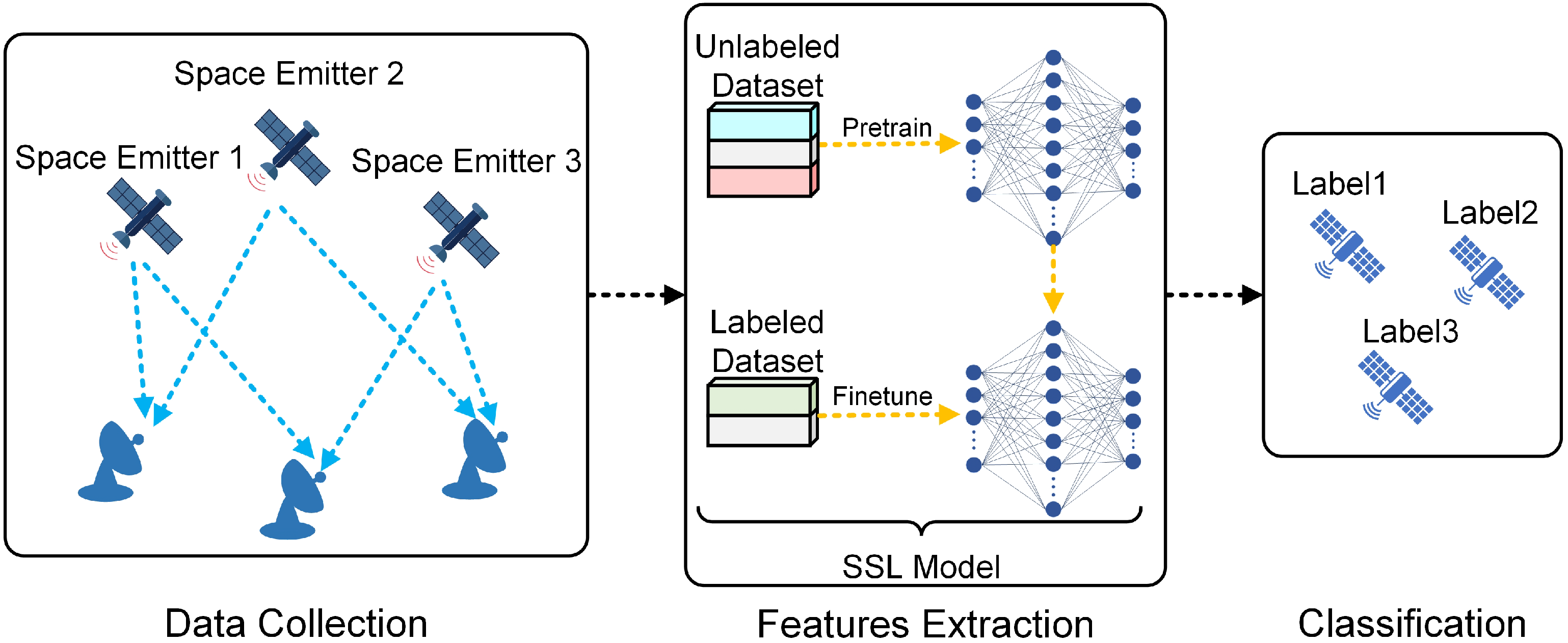
As shown in Figure 1, for radio frequency signals collected from one particular emitter, the identification phase in the SEI system consists of three main steps: data collection, feature extraction, and classification. Considering that it is difficult to collect enough reliable labeled data for driving the training process of RFFs extractor and classifier in real-world scenarios, using unlabeled datasets to construct a self-supervised pretraining task is an effective method. In this paper, it is considered that in the application of real-world scenarios, the datasets of the pretraining phase are unlabeled, and self-supervised contrastive learning is applied to the pretraining task of the RFFs extractor. Subsequently, the pretrained extractor is fine-tuned together with the classifier to tune parameters with the support of limited labeled samples to obtain an end-to-end mapping from input samples to categories.

2.2. Problem Formulation

SSL-SEI aims at achieving high SEI performance with limited labeled samples. The real received space-specific emitter signal $x\left(t\right)$ can be represented as

$$x\left(t\right)=\left[s\left(t\right)*h\left(t\right)+n\left(t\right)\right]·e^{-j2\pi f_{m}t}$$

(1)

where $s\left(t\right)$ denotes the signal containing useful information, $h\left(t\right)$ denotes the pulse response of the channel, and $n\left(t\right)$ denotes the noise and interference during transmission. Additionally, $f_m$ denotes the frequency generated by the mixer to convert a radiofrequency signal into an intermediate frequency signal.

Assume that the sample $\mathbf{x}$ is from an unlabeled dataset ${\mathcal{D}}_{ul}={\left\{{\mathbf{x}}_i\right\}}_{i=1}^N$, where ${\mathbf{x}}_i\in {\mathbb{R}}^L$ denotes a time-domain signal of length L. In this paper, positive and negative sample pairs are generated through data augmentation. Positive samples are defined as two augmented views of the same signal, while negative samples are augmented views of all remaining samples in the same batch.

Using an encoder network $f_{\theta }(·)$ and a neural projection head $g_{\varphi }(·)$, we obtain low-dimensional embedding features:

$${\mathbf{z}}_i=g_{\varphi }\left(f_{\theta }\left({\tilde{\mathbf{x}}}_i\right)\right)\in {\mathbb{R}}^p$$

(2)

where $\theta$ and $\varphi$ denote the parameters of the encoder and projection networks, respectively.

To perform SEI with limited labeled data, a small labeled dataset is introduced to fine-tune the model, defined as ${\mathcal{D}}_l={\left\{({\mathbf{x}}_j,y_j)\right\}}_{j=1}^M$, where ${\mathbf{x}}_j\in {\mathbb{R}}^L$ is a time-domain signal and $y_j\in \{1,2,...,C\}$ denotes its corresponding emitter class label, with C being the number of classes and $M\ll N$.

The goal of the fine-tuning phase is to optimize the feature enhancement module and classifier using the labeled dataset ${\mathcal{D}}_l$, while keeping the pretrained encoder $f_{{\theta }^{*}}$ fixed. The objective is defined as:

$$\underset{\psi ,\omega }{min}{\mathbb{E}}_{({\mathbf{x}}_j,y_j)\sim {\mathcal{D}}_l}{\mathcal{L}}_{\sup }\left(c_{\omega }\left(q_{\psi }\left(f_{{\theta }^{*}}\left({\mathbf{x}}_j\right)\right)\right),y_j\right)$$

(3)

where $({\mathbf{x}}_j,y_j)\sim {\mathcal{D}}_l$ indicates that the sample-label pair $({\mathbf{x}}_j,y_j)$ is drawn from the labeled dataset ${\mathcal{D}}_l$, ${\mathbf{x}}_j$ denotes the signal sample, and $y_j$ is its corresponding class label, $q_{\psi }(·)$ denotes the feature enhancement module and $c_{\omega }(·)$ is the classifier. The function ${\mathcal{L}}_{\sup }(·)$ typically denotes the supervised classification loss used to match predictions to ground-truth labels.

3. Methodology

This section first introduces the overall framework of the proposed method, and then details the various modules of the proposed method.

3.1. Overall Structure

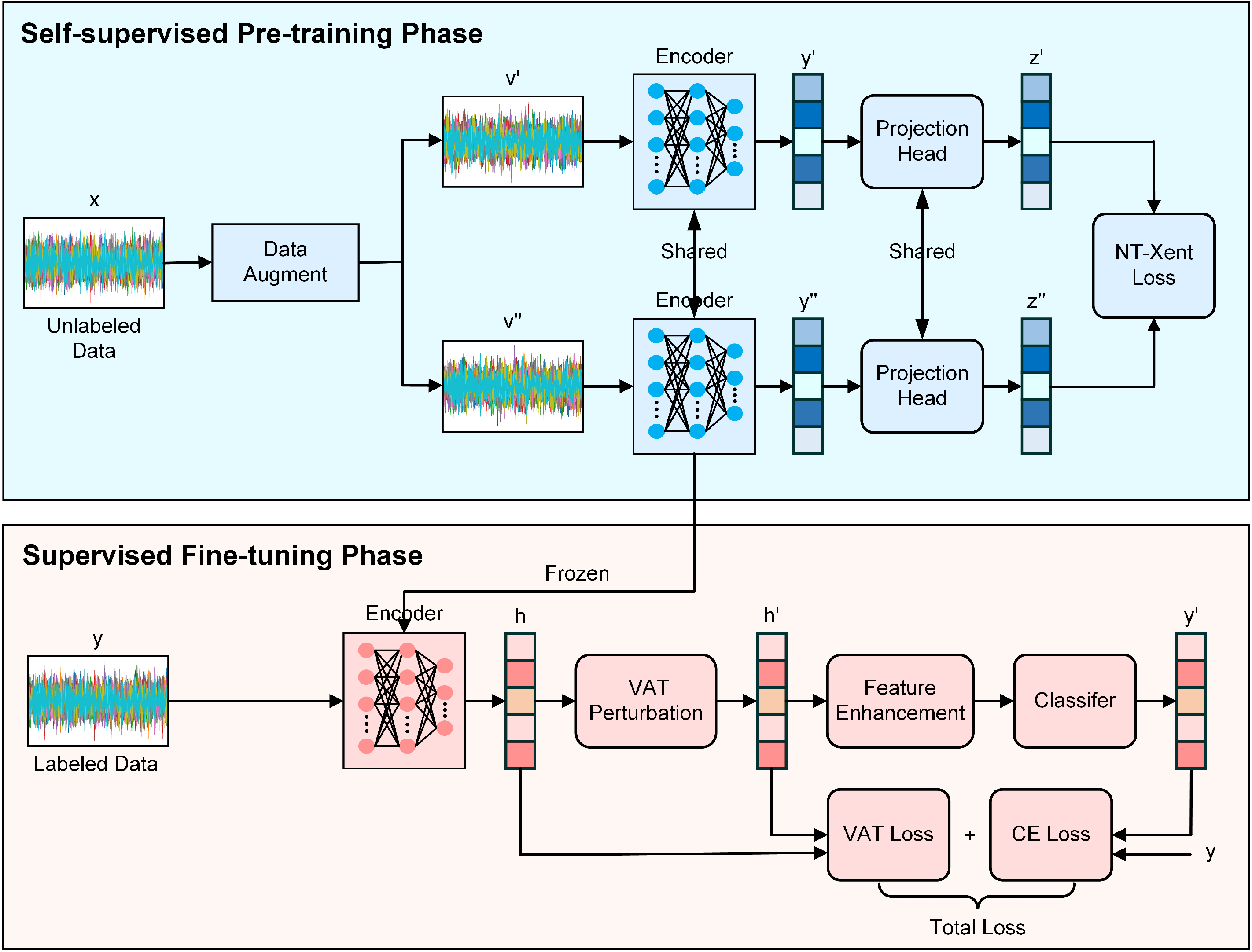
Figure 2 shows the framework of the proposed SSL-SEI method. The proposed method consists of two modules: the self-supervised training module and the fine-tuning classification module. The self-supervised training module includes data augmentation, a ResNet-Transformer hybrid encoder, and a nonlinear projection head. The fine-tuning module consists of a pretrained encoder, a feature enhancement module, and a classifier. Specifically, during the self-supervised training phase, the encoder learns general RFFs through contrastive learning of augmented positive and negative samples. Then, the high-dimensional features are mapped to the low-dimensional contrast space by the projection head. In the fine-tuning stage, adversarial disturbances are introduced into the encoded feature space, and finally, a simple linear classifier is added to optimize the classifier parameters with labeled samples.

3.2. Pretraining Phase

3.2.1. Data Augmentation

Data augmentation is one of the key components in SSL for SEI. It plays a crucial role in constructing positive and negative sample pairs for contrastive learning. To ensure that the extracted RFFs remain invariant to signal content, we design three effective augmentation methods tailored for space-specific emitter signals: Shift, Noise, and Scale. These augmentations introduce diversity while preserving emitter-specific features, thus enabling the model to learn discriminative and robust representations.

Shift: Since RFFs are typically time-invariant, the proposed shift method enhances data diversity by altering the temporal alignment of signals while preserving the underlying RFFs. This helps the model learn more robust and generalizable representations. Unlike general (non-circular) shifts that may lose important parts of the signal, circular shifts retain the complete content, making them particularly suitable for SEI tasks. The proposed shift method circularly shifts the signal by a random offset $\Delta t$ samples,

$${\tilde{\mathbf{x}}}_{\mathrm{shift}}\left[n\right]=\mathbf{x}[(n+\Delta t)modL]$$

(4)

where $\Delta t$ is sampled from a uniform distribution, $\Delta t\sim \mathcal{U}(-100,100)$, and $mod$ denotes the modulo operation, which ensures circular wrapping of indices, thereby preserving the full signal content and avoiding index overflow or truncation.

Noise: To simulate real-world signal impairments such as thermal noise or channel interference, we inject zero-mean Gaussian noise with adaptive intensity, encouraging the model to learn noise-robust features.

$${\tilde{\mathbf{x}}}_{\mathrm{noise}}=\mathbf{x}+\epsilon$$

(5)

where $\epsilon$ is a Gaussian white noise sequence sampled from $\mathcal{N}(0,{\sigma }^{2}I)$, with standard deviation $\sigma =0.05$, corresponding to a 5% perturbation of the signal amplitude.

Scale: To simulate realistic power variations in satellite communication systems caused by transmission power adjustments or dynamic range differences among receivers, we apply randomized linear scaling to the input signals:

$${\tilde{\mathbf{x}}}_{\mathrm{scale}}=\alpha \mathbf{x}$$

(6)

where $\alpha$ is sampled from a uniform distribution, $\alpha \sim \mathcal{U}(0.8,1.2)$.

3.2.2. ResNet-Transformer Hybrid Encoder

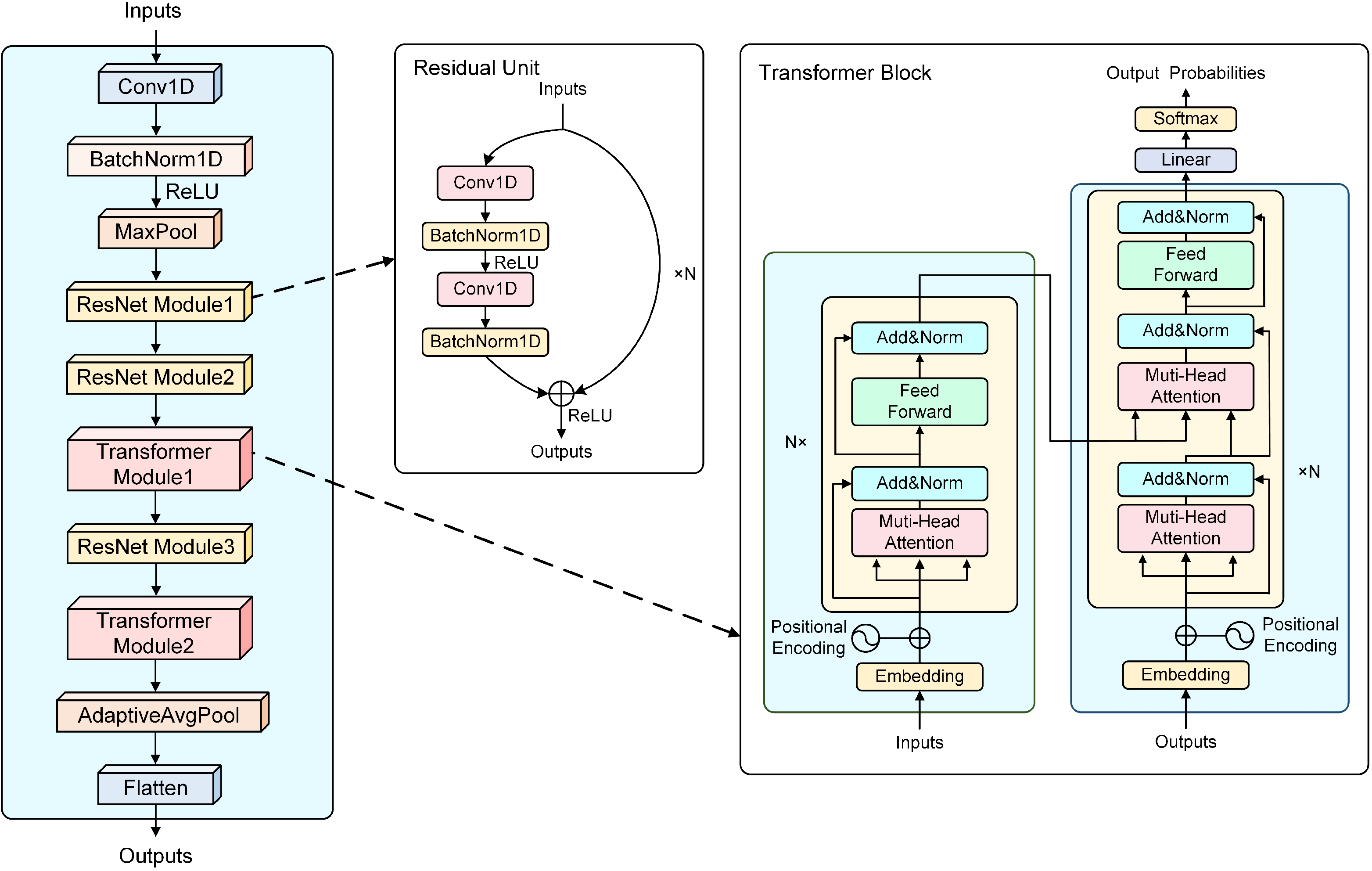
In this paper, a multi-scale spatiotemporal feature fusion encoder is designed, which can jointly capture local and global features of radio frequency signals through alternating stacking of ResNet and Transformer modules. Specifically, for a one-dimensional (1D) raw signal of length L, the model first undergoes 1D convolution, BatchNorm (BN), ReLU activation, and max pooling for embedding to obtain feature vectors. Subsequently, the use of ResNet modules and Transformer modules extracts more robust RFFs from the input feature vectors. Finally, an Adaptive Average Pooling (AdaptiveAvgPool) is applied to compress the temporal dimension to a fixed length, followed by a flatten operation that transforms the resulting tensor into a 1D feature vector. This produces a feature vector of dimension $1\times d$, which is then passed into a nonlinear projection head to map the high-dimensional features into a lower-dimensional contrastive space. Additionally, it uses only the I part of the raw I/Q signal as input, avoiding the extra signal preprocessing step, making it easier to achieve end-to-end training and recognition. Figure 3 shows the specific architecture of the encoder.

The proposed hybrid encoder stacks three ResNet modules and two Transformer modules to hierarchically extract discriminative RFFs, capturing both local features and global temporal dependencies. The three ResNet modules consist of {2, 4, 2} basic residual units, respectively. Each basic residual unit contains two 1D convolutional layers with $7\times 1$ kernels, followed by BN and ReLU activation. Skip connections are incorporated to mitigate gradient vanishing, while adaptive downsampling is applied in the first unit of each module via a $1\times 1$ convolutional layer when the stride or channel dimension changes. After the second and third ResNet modules, Transformer modules with positional encoding and multihead self-attention mechanisms are, respectively, inserted to model long-range interactions in the time domain. The following details the positional encoding and multihead self-attention mechanisms.

Positional encoding: To inject positional information into the Transformer architecture, the absolute position coding defined by the sine function is adopted in this paper. For a given position $pos\in [0,T-1]$ and dimension $i\in [0,d_{model}-1]$, the encoding is computed as:

$$P{E}_{(pos,2i)}=sin\left({\displaystyle \frac{pos}{{10000}^{2i/d_{model}}}}\right)$$

(7)

$$P{E}_{(pos,2i+1)}=cos\left({\displaystyle \frac{pos}{{10000}^{2i/d_{model}}}}\right)$$

(8)

where $d_{model}$ denotes the feature dimension, T is the sequence length. This encoding is added element-wise to the reshaped ResNet output ${\mathbf{h}}_{reshape}\in {\mathbb{R}}^{T\times B\times d_{model}}$ before feeding into the Transformer:

$${\mathbf{h}}_{pos}={\mathbf{h}}_{reshape}+\mathbf{PE}\left(pos\right)$$

(9)

where $\mathbf{PE}\left(pos\right)\in {\mathbb{R}}^{T\times d_{model}}$, B is the batch size, and it is broadcast to $T\times B\times d_{model}$ along the batch dimension to enable element-wise addition with ${\mathbf{h}}_{reshape}$.

Multihead Self-Attention: The implementation of the multihead attention mechanism is divided into three steps:

1.

Linear Projections: Initialize the weight matrices ${\mathbf{W}}^Q,{\mathbf{W}}^K,{\mathbf{W}}^V$, and then calculate the $\mathbf{Q},\mathbf{K},\mathbf{V}$ of each head, respectively,

$$\mathbf{Q}={\mathbf{h}}_{pos}{\mathbf{W}}^Q,\mathbf{K}={\mathbf{h}}_{pos}{\mathbf{W}}^K,\mathbf{V}={\mathbf{h}}_{pos}{\mathbf{W}}^V$$

(10)

where ${\mathbf{W}}^Q,{\mathbf{W}}^K\in {\mathbb{R}}^{d_{model}\times d_k}$, ${\mathbf{W}}^V\in {\mathbb{R}}^{d_{model}\times d_v}$, with $d_k=d_v=d_{model}/n_{heads}$;

2.

Scaled Dot-Product Attention: Each head calculates attention independently,

$$\mathrm{Attention}(\mathbf{Q},\mathbf{K},\mathbf{V})=\mathrm{Softmax}\left({\displaystyle \frac{\mathbf{Q}{\mathbf{K}}^{\top }}{\sqrt{d_k}}}\right)\mathbf{V}$$

(11)

where $\sqrt{d_k}$ represents the scaling factor;

3.

Multihead Concatenation: Project back to the original space through ${\mathbf{W}}^O\in {\mathbb{R}}^{h{d}_v\times d_{model}}$, and then concatenate all the head outputs,

$$\mathrm{MultiHead}(\mathbf{Q},\mathbf{K},\mathbf{V})=\mathrm{Concat}({\mathbf{head}}_1,...,{\mathbf{head}}_h){\mathbf{W}}^O$$

(12)

where h is the number of attention heads.

3.2.3. Nonlinear Projection Head

To facilitate contrastive learning, each feature vector ${\mathbf{h}}_{t,b}\in {\mathbb{R}}^{d_{model}}$, extracted from the encoder output ${\mathbf{h}}_{reshape}$, is independently transformed by a nonlinear projection head $g(·)$. This projection maps the representations into a lower-dimensional latent space to enhance the effectiveness of contrastive objectives. The projection head consists of two fully connected layers with a ReLU activation in between:

$$\mathbf{z}=g\left(\mathbf{h}\right)={\mathbf{W}}^{\left(2\right)}·\mathrm{ReLU}({\mathbf{W}}^{\left(1\right)}\mathbf{h}+{\mathbf{b}}^{\left(1\right)})+{\mathbf{b}}^{\left(2\right)}$$

(13)

where ${\mathbf{W}}^{\left(1\right)}\in {\mathbb{R}}^{d_{model}\times d_{model}}$, ${\mathbf{b}}^{\left(1\right)}\in {\mathbb{R}}^{d_{model}}$, ${\mathbf{W}}^{\left(2\right)}\in {\mathbb{R}}^{d^{\prime }\times d_{model}}$, and ${\mathbf{b}}^{\left(2\right)}\in {\mathbb{R}}^{d^{\prime }}$. Here, $d^{\prime }$ denotes the dimension of the projected latent space, $\mathbf{z}\in {\mathbb{R}}^{d^{\prime }}$ is the final output vector corresponding to each feature position. All projection operations are applied independently to each time step and batch element.

To train the encoder and projection head jointly, we adopt the normalized temperature-scaled cross-entropy (NT-Xent) loss, which encourages the model to bring positive pairs close while pushing apart negative pairs in the projected space. The loss is defined as:

$$\mathcal{L}=-{\displaystyle \frac{1}{2B}}\sum _{k=1}^B\left[log{\displaystyle \frac{exp(s_{k,k+B}/\tau )}{{\sum }_{m=1}^{2B}{1}_{[m\ne k]}exp(s_{k,m}/\tau )}}+log{\displaystyle \frac{exp(s_{k+B,k}/\tau )}{{\sum }_{m=1}^{2B}{1}_{[m\ne k+B]}exp(s_{k+B,m}/\tau )}}\right]$$

(14)

where $s_{i,j}={\mathbf{z}}_i^{\top }{\mathbf{z}}_j/(\parallel {\mathbf{z}}_i\parallel \parallel {\mathbf{z}}_j\parallel )$ denotes the cosine similarity between embeddings $z_i$ and $z_j$, $\tau$ is a temperature parameter that controls the concentration of the similarity distribution, and $1_{m\ne k}\in \{0,1\}$ is an indicator function evaluating to 1 if $\mathit{m}\ne \mathit{k}$. The batch size is denoted by B, and for each anchor k, the corresponding positive sample is at position $k+B$.

3.3. Fine-Tuning Phase

The SEI is a classification task. Therefore, when the SSL phase is over, the encoder network that has learned universal feature representations from unlabeled radiation source signal data can be used as a feature extraction network. In the proposed framework, adversarial perturbations are injected into the output space of the encoder in order to enhance the robustness to the feature distribution shift. Finally, a linear classifier is added to adapt to different downstream classification tasks.

Specifically, after the SSL phase, freeze parameters of the encoder $f(·,\theta )$ as the feature extraction network, where $\theta$ is the frozen parameters. Then, VAT is introduced in the feature space. The specific process is as follows: first of all, sample random noise $d\sim \mathcal{N}(0,{\xi }^{2}I)$, where $\xi ={10}^{-6}$ for initialization. Then, for the feature vector $\mathbf{h}=f(\mathbf{x};\theta )\in {\mathbb{R}}^{256}$ output by the frozen encoder, the adversarial direction is generated through iterative gradient ascent:

$${\mathbf{r}}_{adv}=\underset{{∥\mathbf{r}∥}_2\le \epsilon }{argmax}{D}_{KL}(p\left(y\right|\mathbf{h})\parallel p\left(y\right|\mathbf{h}+\mathbf{r}))$$

(15)

where $\epsilon$ controls perturbation magnitude, $p\left(y\right|\mathbf{h})$ denotes original prediction distribution, $p\left(y\right|\mathbf{h}+\mathbf{r})$ denotes perturbed prediction distribution, “∥” denotes the KL divergence between two probability distributions, and KL divergence measures the difference in classification distribution before and after feature perturbation. Then calculate the VAT loss:

$${\mathcal{L}}_{VAT}={\mathbb{E}}_x\left[D_{KL}(p\left(y\right|\mathbf{h})\parallel p\left(y\right|\mathbf{h}+{\mathbf{r}}_{adv}))\right]$$

(16)

Finally, a lightweight network $q_{\psi }$ is appended to adapt features for downstream tasks:

$${\mathbf{h}}_{enh}=Dropout\left(GeLU\left(LayerNorm({\mathbf{W}}_f\mathbf{h}+{\mathbf{b}}_f)\right)\right)$$

(17)

where ${\mathbf{W}}_f$, ${\mathbf{b}}_f$, and $\mathbf{h}$ is the frozen encoder output. Furthermore, a linear layer $c_{\omega }$ is used as a classifier to map the enhanced features to the class logic.

The total loss combines cross-entropy and VAT regularization:

$${\mathcal{L}}_{CE}={\displaystyle \frac{1}{N}}\sum _{i=1}^N-logp\left(y_i\right|{\mathbf{x}}_i)$$

(18)

$${\mathcal{L}}_{total}={\mathcal{L}}_{CE}+\lambda {\mathcal{L}}_{VAT}$$

(19)

where $\lambda$ is a weighting factor that determines the intensity of regularization, y denotes the ground-truth label.

3.4. Description of the Algorithm

The proposed framework operates in two stages: self-supervised pretraining for generic feature learning and supervised fine-tuning for task-specific adaptation.

Pretraining Phase: Leveraging unlabeled RF signals, the model learns discriminative representations through contrastive learning. Input signals undergo data augmentation to generate positive and negative pairs, which are encoded by the hybrid encoder. A nonlinear projection head maps encoded features to a lower-dimensional space where NT-Xent loss maximizes agreement between positive pairs while repelling negatives.

Fine-tuning Phase: The pretrained encoder is frozen to preserve general features. A lightweight feature enhancement module and linear classifier are appended. VAT injects worst-case perturbations into the frozen encoder’s feature space to enhance robustness, combining cross-entropy classification loss with VAT loss. The specific pseudocode is shown in Algorithm 1.

Algorithm 1: Self-Supervised SEI Framework

Pretraining Phase   Input: Unlabeled dataset ${\mathcal{D}}_{ul}={\left\{{\mathbf{x}}_i\right\}}_{i=1}^N$, where ${\mathbf{x}}_i\in {\mathbb{R}}^{4000}$   Parameters: Encoder $f_{\theta }$, Projection head $g_{\varphi }$ 1: for epoch $=1$ to $N_{pretrain}$ do 2:     for each batch ${\left\{{\mathbf{x}}_k\right\}}_{k=1}^B\subset {\mathcal{D}}_{ul}$ do 3:         Generate two augmented views: ${\tilde{\mathbf{x}}}_i\leftarrow {\mathcal{T}}_1\left({\mathbf{x}}_k\right)$, ${\tilde{\mathbf{x}}}_j\leftarrow {\mathcal{T}}_2\left({\mathbf{x}}_k\right)$ 4:         Extract representations: ${\mathbf{h}}_i\leftarrow f_{\theta }\left({\tilde{\mathbf{x}}}_i\right)$, ${\mathbf{h}}_j\leftarrow f_{\theta }\left({\tilde{\mathbf{x}}}_j\right)$ 5:         Project features: ${\mathbf{z}}_i\leftarrow g_{\varphi }\left({\mathbf{h}}_i\right)$, ${\mathbf{z}}_j\leftarrow g_{\varphi }\left({\mathbf{h}}_j\right)$ 6:         Compute similarity: $\mathrm{sim}(\mathbf{u},\mathbf{v})\leftarrow {\displaystyle \frac{{\mathbf{u}}^{\top }\mathbf{v}}{\parallel \mathbf{u}\parallel \parallel \mathbf{v}\parallel }}$ 7:         Compute contrastive loss ${\mathcal{L}}_{cont}$ as Equation (14) 8:         Update parameters: $$\theta \leftarrow \theta -{\eta }_{\theta }{\nabla }_{\theta }{\mathcal{L}}_{cont},\varphi \leftarrow \varphi -{\eta }_{\varphi }{\nabla }_{\varphi }{\mathcal{L}}_{cont}$$ 9:     end for 10: end for   Fine-tuning Phase   Input: Labeled dataset ${\mathcal{D}}_l={\left\{({\mathbf{x}}_j,y_j)\right\}}_{j=1}^M$, $y_j\in \{1,\dots ,C\}$   Parameters: Frozen encoder $f_{{\theta }^{*}}$, Feature enhancement module $q_{\psi }$, Classifier $c_{\omega }$ 11: for epoch $=1$ to $N_{finetune}$ do 12:     for each batch ${\left\{({\mathbf{x}}_k,y_k)\right\}}_{k=1}^B\subset {\mathcal{D}}_l$ do 13:         Feature extraction and enhancement: $$\mathbf{h}\leftarrow f_{{\theta }^{*}}\left({\mathbf{x}}_k\right),{\mathbf{h}}_{\mathrm{enh}}\leftarrow q_{\psi }\left(\mathbf{h}\right),\widehat{y}\leftarrow c_{\omega }\left({\mathbf{h}}_{\mathrm{enh}}\right)$$ 14:         Compute cross-entropy loss ${\mathcal{L}}_{CE}$ as Equation (18) 15:         Generate random noise: $d\sim \mathcal{N}(0,{\xi }^{2}I)$ 16:         Compute adversarial direction ${\mathbf{r}}_{adv}$ as Equation (15) 17:         Compute VAT loss ${\mathcal{L}}_{VAT}$ as Equation (16) 18:         Compute total loss ${\mathcal{L}}_{total}$ as Equation (19) 19:         Update parameters: $$\psi \leftarrow \psi -{\eta }_{\psi }{\nabla }_{\psi }{\mathcal{L}}_{\mathrm{total}},\omega \leftarrow \omega -{\eta }_{\omega }{\nabla }_{\omega }{\mathcal{L}}_{\mathrm{total}}$$ 20:     end for 21: end for

4. Experimental Results Analysis and Discussion

4.1. Datasets

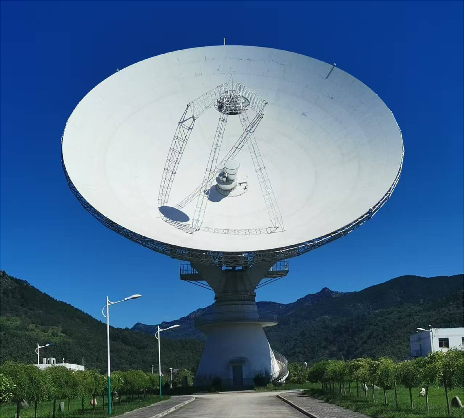
In order to validate the effectiveness of the proposed method, we collected real-world satellite navigation signals using a 40-m antenna, as shown in Figure 4, and conducted extensive experiments. These data are from the BDS signals and contain 10 different categories, labeled from 0 to 9. Each sample is a 1D sequence of length 4000, and its shape is $1\times 4000$. In the pretraining stage, each class has 800 samples, totaling 8000 training samples. This ensures that the encoder learns generalizable representations of all categories without label supervision. During the fine-tuning stage, we simulated a limited labeled data scenario. The number of labeled samples per class was varied across experiments, taking values from the set $\{10,15,20,25,30,35,40\}$, to evaluate model performance under different levels of supervision. For each scenario, the labeled data are randomly divided into the training set and the validation set, with a ratio of 0.8:0.2, respectively. The test set remained fixed throughout all experiments and consisted of 1500 samples, ensuring consistent and fair evaluation across all models.

To ensure a fair and objective evaluation, the pretraining dataset (unlabeled) and the fine-tuning dataset (labeled) are strictly non-overlapping. Specifically, the unlabeled data used during the self-supervised pretraining stage is entirely separate from the labeled data used in the fine-tuning stage. Furthermore, within the fine-tuning process, the training, validation, and test sets are constructed independently without any shared samples. This strict separation prevents data leakage and ensures that the experimental results accurately reflect the validity of the model. The details of the datasets are shown in

Table 1. Details of BDS signal datasets for pretraining and fine-tuning.

Parameters	Pretraining	Fine-Tuning
Number of classes	10 (0–9)	10 (0–9)
Dimension of samples	$1\times 4000$	$1\times 4000$
Number sample of per class	800	{10,15,20,25,30,35,40}
Train/Valid ratio	-	(0.8,0.2)
Test set	-	$1500\times 4000$

.

4.2. Experimental Details

All experiments were implemented using Python 3.9.19 and the PyTorch 1.11 framework. Training was conducted on a workstation equipped with an NVIDIA GeForce RTX 4090 GPU. For the self-supervised pretraining stage, we trained the model for 200 epochs using the LARS optimizer, with a batch size of 256 and a learning rate set to $5\times {10}^{-2}$. The temperature parameter $\tau$ in the contrastive loss is set to 0.1. During the fine-tuning stage, we trained for 100 epochs using a smaller batch size of 32, and adopted the Adam optimizer with a learning rate of $5\times {10}^{-4}$ for stable convergence. The test batch size was also set to 32 to match the training configuration during evaluation. The VAT weight ($\lambda$) is set to 0.3, and the perturbation magnitude ($\epsilon$) is set to 4.0. These values are selected to balance the trade-off between task loss and adversarial smoothing. The selection principle of VAT parameters will be discussed in detail in Section 4.6. The details and simulation parameters are shown in

Table 2. Parameter settings of SSL-SEI.

Parameters	Self-Supervised Training	Fine-Tuning
Python	3.9.19
PyTorch	1.11
Platform	NVIDIA GeForce RTX 4090 GPU
Epochs	200	100
Training Batch Size	256	32
Test Batch Size	-	32
Optimizer	LARS	Adam
Learning Rate	$5\times {10}^{-2}$	$5\times {10}^{-4}$
Temperature ($\tau$)	0.1	-
VAT Weight ($\lambda$)	-	0.3
VAT Perturbation ($\epsilon$)	-	4.0

.

We use four widely used evaluation metrics for SEI, including Accuracy (ACC), Recall (R), Precision (P), and F1-score (F). Among them, Accuracy, Recall, Precision, and F1-score range from 0 to 1. It is worth noting that a higher value of all metrics indicates better performance of the model. These evaluation metrics are defined as follows:

Accuracy (ACC): Accuracy measures the proportion of correct predictions out of the total number of predictions. It is defined as:

$$ACC={\displaystyle \frac{TP+TN}{TP+TN+FP+FN}}$$

(20)

where $TP$ represents the number of true positives, $TN$ represents the number of true negatives, $FP$ represents the number of false positives, and $FN$ represents the number of false negatives.

Recall (R): Recall measures the proportion of actual positives that are correctly identified:

$$R={\displaystyle \frac{TP}{TP+FN}}$$

(21)

Precision (P): Precision measures the proportion of positive predictions that are actually correct:

$$P={\displaystyle \frac{TP}{TP+FP}}$$

(22)

F1-score (F): The F1-score is the harmonic mean of precision and recall. It provides a balance between the two metrics:

$$F={\displaystyle \frac{2\times P\times R}{P+R}}$$

(23)

4.3. Comparison Methods

To verify the effectiveness of the proposed method, four comparative methods are introduced as follows.

1.

FineZero: FineZero indicates that it directly trains the RFFs extractor and classifier without going through the pretraining stage, where the RFFs extractor is the hybrid encoder proposed in this paper. Specifically, there is no knowledge transfer during the training process, and the parameters of the RFFs extractor and classifier are randomly initialized. Therefore, the performance of FineZero represents the performance baseline.

2.

MAML: MAML [39] is a model-agnostic meta-learning framework that aims to quickly adapt to new tasks with a small number of samples. The core idea is to learn a common set of initialization parameters so that the model can efficiently solve new tasks with a small number of gradient updates.

3.

SimCLR: SimCLR [40] is a self-supervised contrastive learning method. SimCLR takes the augmented views of samples as positive examples and all other samples in a batch as negative examples.

4.

SA2SEI: SA2SEI [34] is a few-shot SEI method based on self-supervised learning and adversarial enhancement. Specifically, a novel adversarial enhancing-driven self-supervised learning is used to pretrain the RFFs extractor with unlabeled auxiliary datasets, and knowledge transfer is introduced to fine-tune the extractor and classifier.

Table 3. Accuracy comparison of various methods.

Methods	{10}	{15}	{20}	{25}	{30}	{35}	{40}
Baseline	40.93%	48.67%	60.27%	60.60%	68.20%	79.27%	80.93%
MAML	36.67%	55.52%	68.52%	72.06%	76.56%	81.06%	82.45%
SimCLR	49.93%	57.53%	70.93%	75.27%	80.53%	83.93%	86.00%
SA2SEI	43.13%	50.53%	68.43%	79.12%	83.06%	88.54%	91.08%
Proposed	54.73%	64.93%	89.27%	94.27%	95.93%	97.07%	97.20%

presents the performance comparison of various methods applied to the BDS signal datasets across different scenarios ({10,15,20,25,30,35,40}-shot). The experimental results show that the proposed method significantly outperforms other methods on the BDS signal datasets.

As shown by the experimental results in Table 3, the proposed method consistently achieves significantly higher identification accuracy than existing mainstream approaches across all training sample settings. In the 10-shot setting, the proposed method reaches an accuracy of 54.73%, outperforming SimCLR (49.93%), SA2SEI (43.13%), MAML (36.67%), and the baseline (40.93%). As the number of training samples increases, the performance of the proposed method improves at a much faster rate than other methods. For instance, under the 20-shot setting, it achieves 89.27% accuracy, whereas SimCLR reaches 70.93%, SA2SEI 68.43%, MAML 68.52%, and the baseline only 60.27%. This pronounced performance gap demonstrates the effectiveness of the proposed framework in enabling the model to capture discriminative features even when labeled data are limited. Under larger sample settings ({25,30,35,40}-shot), the proposed method continues to maintain a strong lead, ultimately achieving an accuracy of 97.20% in the 40-shot setting, significantly surpassing SA2SEI (91.08%), SimCLR (86.00%), and all other methods.

In addition to accuracy, we also evaluate the performance of the model in terms of recall, precision, and F1-score, as shown in

Table 4. Recall comparison of various methods.

Methods	{10}	{15}	{20}	{25}	{30}	{35}	{40}
Baseline	39.85%	47.52%	59.15%	59.80%	67.05%	78.12%	79.87%
MAML	35.62%	54.30%	67.25%	70.88%	75.33%	79.95%	81.40%
SimCLR	48.75%	56.40%	69.75%	74.05%	79.25%	82.75%	84.85%
SA2SEI	42.05%	49.45%	67.25%	77.95%	81.90%	87.40%	89.95%
Proposed	53.65%	63.75%	88.05%	93.15%	94.85%	96.00%	96.15%

,

Table 5. Precision comparison of various methods.

Methods	{10}	{15}	{20}	{25}	{30}	{35}	{40}
Baseline	38.61%	44.31%	60.41%	60.64%	68.11%	80.08%	81.04%
MAML	41.51%	61.30%	72.49%	72.73%	76.52%	81.20%	82.64%
SimCLR	48.97%	62.65%	71.20%	75.43%	80.76%	84.27%	86.83%
SA2SEI	43.07%	50.91%	68.41%	78.82%	83.29%	89.04%	91.12%
Proposed	54.20%	67.08%	91.15%	94.47%	96.13%	97.27%	97.60%

and

Table 6. F1-score comparison of various methods.

Methods	{10}	{15}	{20}	{25}	{30}	{35}	{40}
Baseline	36.58%	43.71%	58.81%	60.25%	68.44%	79.40%	81.23%
MAML	39.97%	61.09%	71.98%	72.06%	76.37%	80.98%	82.01%
SimCLR	48.03%	61.72%	70.72%	75.25%	80.52%	83.95%	86.06%
SA2SEI	43.15%	50.37%	68.85%	79.30%	83.18%	88.51%	90.89%
Proposed	53.05%	65.28%	89.48%	94.29%	95.97%	97.08%	97.44%

. The proposed method consistently achieves the highest values on all three metrics across all shot settings. For example, in the 20-shot scenario, the proposed method achieves 88.05% recall, 91.15% precision, and 89.48% F1-score, substantially outperforming all comparison methods. This trend persists across increasing sample sizes, culminating in 40-shot scores of 96.15% recall, 97.60% precision, and 97.44% F1-score. These results further validate the robustness and effectiveness of the proposed approach from multiple evaluation perspectives.

Overall, these results indicate that the proposed approach offers high precision and robustness in scenarios with limited labeled data. The experimental results validate the effectiveness of the introduced hybrid encoder architecture, the self-supervised contrastive learning mechanism, and the VAT-based fine-tuning strategy for the SEI task.

4.4. Exploring the Impact of Different Data Augmentation Strategies on SSL

To investigate the impact of different data augmentation strategies on the effectiveness of self-supervised pretraining, we conducted a series of experiments using various augmentation combinations. All experiments use the same parameter settings described in Section 4.2. The experimental results are shown in Figure 5.

The results demonstrate that single augmentations, such as Noise, Scale, or Shift, generally provide moderate improvements as the number of labeled samples increases. Among them, the Scale and Shift augmentations outperform Noise, achieving 96.93% and 92.53% accuracy, respectively, at 40 labeled samples per class, compared to 75.87% for Noise. This suggests that geometric transformations (Scale and Shift) are more beneficial for representation learning than random Noise alone. The improvement trend shown by pairwise enhancement combinations, including Noise + Scale, Noise + Shift, and Scale + Shift, is not very stable, and these combinations only outperform single enhancements under specific sample sizes. The proposed enhancement strategy (Noise + Scale + Shift) consistently outperforms all other configurations in all sample sizes. It achieves the highest accuracy rate of 97.20% when there are 40 samples in each class. More importantly, it demonstrates a significant leading advantage in low-resource scenarios. The above experimental results demonstrate the effectiveness of the data augmentation proposed in this study in the SSL phase.

4.5. Ablation Experiment

As shown in

Table 7. Classification accuracy of various ablation variants.

Model Variant	Top-1 Acc (%)
(A) ResNet Only	73.93%
(B) Hybrid Encoder Only	80.93%
(C) ResNet + SSL	86.00%
(D) Hybrid Encoder + SSL	89.67%
(E) ResNet + SSL + VAT	92.87%
(F) Proposed	97.20%

, we conducted ablation experiments in the 10-class BDS signal dataset under the 40-shot scenario to evaluate the effectiveness of each component in the framework we proposed. All experiments use the same parameter settings described in Section 4.2. Model (A) adopts the RFFs extractor modified based on the ResNet-50. This model is trained in a supervised learning manner without going through any self-supervised pretraining stage, and uses cross-entropy loss for end-to-end optimization. Model (B) uses the hybrid encoder proposed in this paper instead of ResNet and adopts the same training strategy as Model (A). Models (C) and (E) use the same encoder as Model (A), adopt the self-supervised training strategy, and introduce contrastive learning. Model (E) further introduces the VAT-based fine-tuning method proposed in this paper. Model (D) uses the same encoder as Model (B), adopts a self-supervised training strategy, and introduces contrastive learning. Model (F) is the method proposed in this paper.

1.

Effectiveness Analysis of Hybrid Encoder: The hybrid encoder leverages ResNet to extract local signal features and Transformer to capture global dependencies via self-attention. This combination leads to more expressive and generalizable RFF representations for SEI. To validate the effectiveness of the proposed hybrid encoder architecture, we compare pairs of models trained under identical strategies but with different encoders. Specifically, comparing (A) and (B), the accuracy improves from 73.93% to 80.93%, indicating that the hybrid encoder provides a more expressive representation than the vanilla ResNet. Similarly, under the SSL setting, (C) achieves 86.00%, while (D) achieves 89.67%, again demonstrating consistent performance gains from the hybrid encoder. Finally, under the full framework including both SSL and VAT, (E) achieves 92.87%, whereas (F) reaches 97.20%, further highlighting the contribution of the hybrid encoder to overall performance improvement.

2.

Effectiveness Analysis of SSL: The SSL framework guides the model to learn invariant and discriminative features by maximizing agreement between augmented views of the same signal. This contrastive objective encourages the encoder to enhance RFF extraction without relying on labels. To evaluate the impact of the SSL framework, we compare models with and without SSL while keeping the encoder fixed. For the ResNet-based models, (A) achieves 73.93%, whereas (C) improves to 86.00%, indicating that the introduction of the SSL framework achieved a significant gain of nearly 10%. A similar trend is observed with the hybrid encoder: (B) achieves 80.93%, while (D) achieves 89.67%. These results confirm that the self-supervised framework effectively improves feature representations by leveraging unlabeled data, especially when labeled samples are limited.

3.

Effectiveness Analysis of VAT: VAT improves model robustness by introducing small adversarial perturbations, encouraging the classifier to maintain consistent predictions around labeled samples. This regularization smooths decision boundaries and prevents overfitting, which is crucial for SEI tasks under limited labeled data. To investigate the contribution of VAT, we compare models trained with and without VAT under the SSL setting. When using the ResNet encoder, (C) achieves 86.00%, while (E) improves to 92.87%. Similarly, with the hybrid encoder, performance increases from 89.67% in (D) to 97.20% in (F). These results demonstrate that VAT effectively enhances the model’s robustness and generalization, particularly when combined with the hybrid encoder and SSL components.

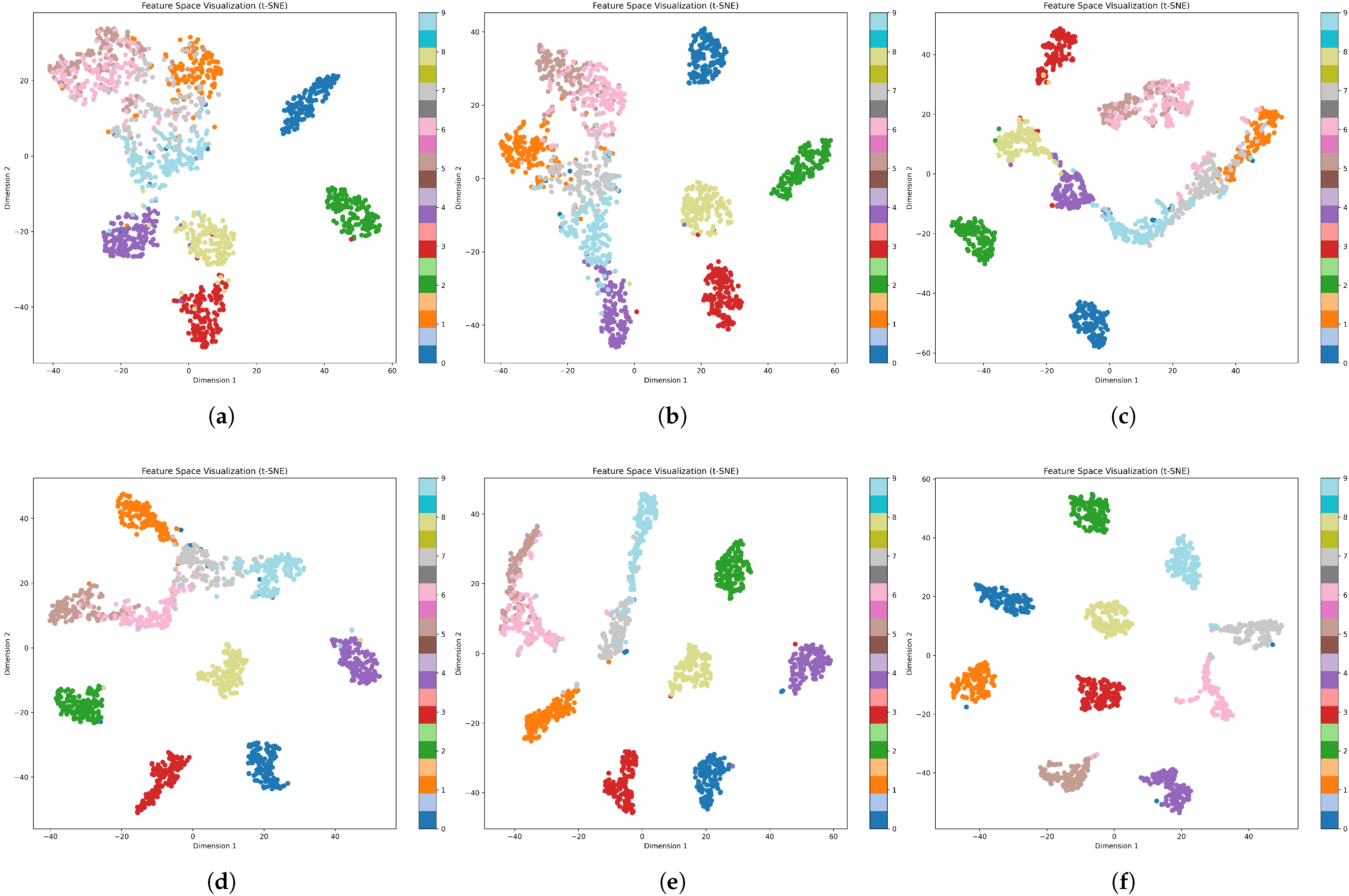
To further investigate the discriminative capability of the learned representations, we performed t-SNE visualization on the feature embeddings of all models. Figure 6 presents the scatter plots of features from 10 selected classes in the BDS signal datasets, extracted by different models. For models (A) and (B) without SSL or VAT, the clusters show obvious overlap and relatively poor intra-class compactness, indicating limited discriminative ability. After the introduction of self-supervised learning, (C) and (D) exhibit a more compact intra-class distribution and better inter-class separation, indicating that the SSL framework effectively guides the encoder to learn semantically meaningful representations. With the introduction of VAT, it was observed that (E) further demonstrated clearer class boundaries and a more compact intra-class distribution than the model using only SSL. Finally, the complete Model (F) achieves the best visualization quality, featuring highly compact intra-class clusters and minimal inter-class overlap. This clear and well-separated feature distribution reflects the effectiveness of each component and proves that the proposed complete framework not only achieves high precision but also learns a highly discriminative feature space.

Table 8. Comparison of silhouette coefficient and separation ratio for various ablation variants.

Model Variant	Silhouette Coefficient	Separation Ratio
(A) ResNet Only	0.2440	2.2968
(B) Hybrid Encoder Only	0.3281	2.1159
(C) ResNet + SSL	0.3559	2.4461
(D) Hybrid Encoder + SSL	0.5109	2.6426
(E) ResNet + SSL + VAT	0.6008	3.4065
(F) Proposed	0.8859	11.3587

further quantitatively analyzes the silhouette coefficient and separation ratio. Specifically, we use the silhouette coefficient and separation ratio to measure the distribution of class representations. The silhouette coefficient measures separation quality between clusters, and the higher values (closer to 1) indicate better clustering, which is defined as:

$$s={\displaystyle \frac{1}{n}}\sum _{i=1}^n{\displaystyle \frac{b\left(i\right)-a\left(i\right)}{max\left\{a\left(i\right),b\left(i\right)\right\}}}$$

(24)

where $a\left(i\right)$ represents average Euclidean distance between sample i and all other points in the same cluster, $b\left(i\right)$ represents the smallest average Euclidean distance between sample i and points in any other cluster, and n is total number of samples.

The separation ratio is the ratio of inter-cluster separation to intra-cluster compactness. Higher values indicate superior clustering (well-separated and tight clusters). The separation ratio is defined as:

$$SepRatio={\displaystyle \frac{InterSep}{IntraCompact+ϵ}}$$

(25)

where $ϵ$ is a small constant to prevent division by zero. Intra-class compactness and inter-class separation, respectively, represent the average distance of samples within the cluster and the average distance of the cluster centroids, and are defined as:

$$IntraCompact={\displaystyle \frac{1}{N_p}}\sum _{k=1}^K\sum _{\begin{array}{c}i,j\in C_k\\ i<j\end{array}}d({\mathbf{x}}_i,{\mathbf{x}}_j)$$

(26)

$$InterSep={\displaystyle \frac{1}{M_p}}\sum _{1\le p<q\le K}d({\mu }_p,{\mu }_q)$$

(27)

where $C_k$ is the set of samples in cluster k ($k=1,\dots ,K$), $d({\mathbf{x}}_i,{\mathbf{x}}_j)$ is the Euclidean distance between samples ${\mathbf{x}}_i$ and ${\mathbf{x}}_j$, $N_p$ is the total intra-cluster pairs, ${\mu }_k$ is the centroid of cluster k, $d({\mu }_p,{\mu }_q)$ is the Euclidean distance between centroids, and $M_p$ is the total cluster pairs.

As shown in Table 8, (A) and (B) yield the lowest silhouette coefficients and separation ratios, indicating poor feature discrimination and clustering quality. The incorporation of self-supervised learning in (C) and (D) leads to consistent improvements across both metrics, demonstrating the effectiveness of contrastive pretraining in enhancing representation learning. Further performance gains are achieved with the addition of VAT in Model (E), highlighting its role in improving robustness and inter-class separability under limited supervision. The complete Model (F) achieves the highest silhouette coefficient of 0.8859 and a separation ratio of 11.3587, significantly outperforming all other variants.

These results collectively validate the effectiveness of the proposed SSL-SEI framework. By integrating contrastive pretraining with VAT-based fine-tuning, the framework successfully learns highly discriminative and robust feature representations, enabling accurate emitter identification even with limited labeled data.

4.6. Impact of VAT Parameters

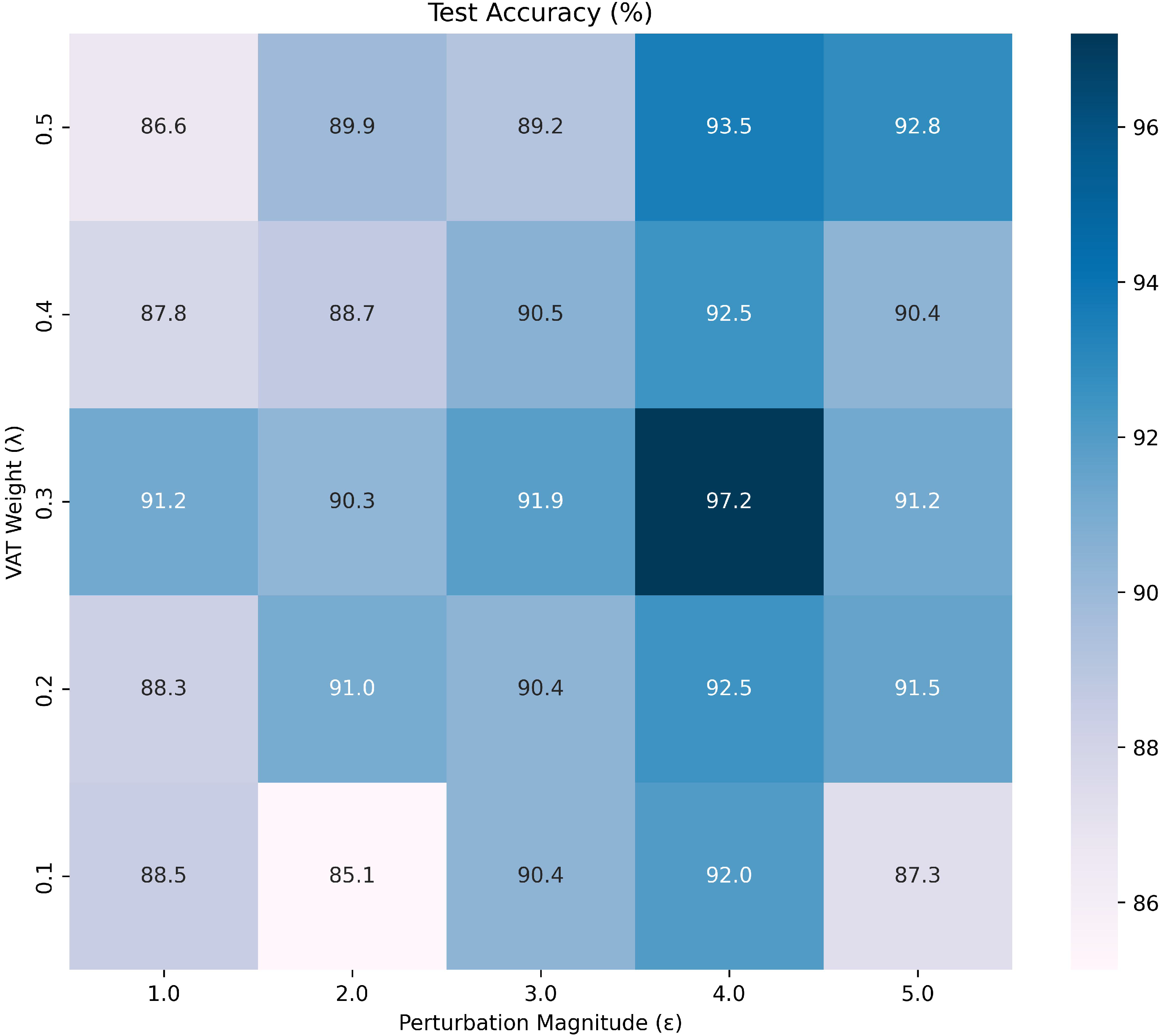
To evaluate the sensitivity of VAT parameters, we conducted a comprehensive grid search analysis of perturbation magnitude ($\epsilon$) and VAT weight ($\lambda$) in the 10-class BDS signal dataset under the 40-shot scenario. Figure 7 presents a heat map illustrating the results of a grid search conducted to evaluate the sensitivity of $\epsilon$ and $\lambda$.

The experimental results indicate that under the condition of fixed $\lambda$, the recognition accuracy shows a trend of first increasing and then slowly decreasing with the increase of $\epsilon$. Among them, $\epsilon =4.0$ reaches the peak across different $\lambda$ settings, indicating that moderately enhancing the perturbation is beneficial to improving the robustness of the model. It is worth noting that a larger disturbance intensity ($\epsilon =\{3.0,4.0\}$) is generally superior to a smaller intensity ($\epsilon =\{1.0,2.0\}$), but an appropriate $\lambda$ needs to be set to achieve the best performance. This aligns with the theoretical of VAT, when $\epsilon$ is too small ($\epsilon =1.0,2.0$), the perturbation fails to sufficiently explore the decision boundary, limiting its regularization effect. Conversely, overly large perturbations ($\epsilon =5.0$) distort the input signal representation beyond the manifold of valid samples, leading to performance degradation. The optimal range, observed at $\epsilon =3.0,4.0$, achieves a balance between boundary exploration and feature integrity. This is consistent with VAT theory, where moderate perturbations enforce local smoothness without destroying the discriminative structure.

The VAT loss is weighted by the coefficient $\lambda$, which controls the influence of the virtual adversarial regularization term relative to the supervised loss. A smaller value of $\lambda$ (e.g., 0.1) fails to sufficiently emphasize the VAT regularization, potentially leading to overfitting in data-scarce settings. On the other hand, excessively large values (e.g., $\lambda \ge 0.4$) may overly constrain the model, interfering with supervised learning and resulting in underfitting. The best performance is observed with $\lambda =0.3$, which achieves an optimal trade-off between maintaining decision boundary smoothness and preserving discriminative learning capacity.

In summary, the optimal configuration ($\epsilon =4.0$, $\lambda =0.3$) aligns with the theoretical design of VAT, providing both sufficient boundary exploration and stability.

4.7. Impact of Environmental Diversity on Model Performance

To evaluate the adaptability and robustness of the proposed method under real-world conditions, we define the dataset described in Section 4.1 as Dataset1, and construct five additional datasets (Dataset2 through Dataset6) using signal data collected from the same 10 BDS satellites over a long time span from 2021 to 2024. These satellites were observed under varying temporal and orbital conditions, naturally introducing environmental variability such as changes in satellite hardware states, signal propagation conditions, and ground station configurations.

It is worth noting that in these supplementary experiments, we retain the model pretrained on Dataset1 and perform fine-tuning using only a small number of labeled samples from each of the new datasets. This setup reflects practical deployment scenarios where a general-purpose feature extractor, once pretrained, can be rapidly adapted to newly collected data without retraining from scratch. Instead, only minimal labeled data are required to fine-tune the model for evolving signal environments. Evaluation metrics, including Accuracy (ACC), Precision (P), Recall (R), and F1-score (F), are used to quantify classification performance across the datasets.

As shown in

Table 9. Accuracy comparison of various datasets.

Dataset	{10}	{15}	{20}	{25}	{30}	{35}	{40}
Dataset1	54.73%	64.93%	89.27%	94.27%	95.93%	97.07%	97.20%
Dataset2	51.40%	69.67%	81.33%	83.40%	85.07%	92.67%	94.73%
Dataset3	51.93%	71.00%	79.73%	89.93%	92.07%	95.07%	97.00%
Dataset4	60.40%	72.33%	77.67%	86.53%	85.67%	97.27%	98.40%
Dataset5	43.33%	52.27%	76.13%	85.13%	87.07%	95.20%	95.60%
Dataset6	51.00%	52.33%	76.27%	91.47%	94.87%	96.73%	96.27%

,

Table 10. Recall comparison of various datasets.

Dataset	{10}	{15}	{20}	{25}	{30}	{35}	{40}
Dataset1	53.65%	63.75%	88.05%	93.15%	94.85%	96.00%	96.15%
Dataset2	48.34%	75.95%	80.36%	82.60%	82.00%	90.47%	93.59%
Dataset3	47.23%	69.21%	77.49%	85.64%	91.88%	94.86%	96.96%
Dataset4	56.72%	68.80%	74.47%	84.04%	83.50%	97.17%	98.37%
Dataset5	40.47%	49.91%	74.21%	82.77%	84.67%	95.13%	95.31%
Dataset6	48.30%	50.42%	73.37%	91.21%	94.58%	96.71%	96.19%

,

Table 11. Precision comparison of various datasets.

Dataset	{10}	{15}	{20}	{25}	{30}	{35}	{40}
Dataset1	54.20%	67.08%	91.15%	94.47%	96.13%	97.27%	97.60%
Dataset2	50.63%	83.15%	82.65%	83.75%	88.35%	93.91%	95.91%
Dataset3	54.88%	72.78%	81.94%	93.32%	92.14%	95.41%	97.07%
Dataset4	64.70%	75.11%	81.27%	88.65%	87.89%	97.31%	98.43%
Dataset5	44.96%	53.58%	78.23%	87.98%	89.14%	95.26%	95.69%
Dataset6	51.97%	51.76%	77.48%	91.70%	95.05%	96.75%	96.29%

and

Table 12. F1-score comparison of various datasets.

Dataset	{10}	{15}	{20}	{25}	{30}	{35}	{40}
Dataset1	53.05%	65.28%	89.48%	94.29%	95.97%	97.08%	97.44%
Dataset2	49.47%	79.47%	81.50%	83.17%	85.07%	92.13%	94.72%
Dataset3	50.89%	70.83%	79.68%	89.39%	92.01%	95.13%	97.02%
Dataset4	60.45%	71.97%	77.80%	86.29%	85.62%	97.24%	98.40%
Dataset5	42.63%	51.67%	76.16%	85.28%	86.81%	95.19%	95.50%
Dataset6	50.11%	51.10%	75.39%	91.45%	94.81%	96.73%	96.24%

, the proposed model consistently maintains strong performance across all datasets. While a slight reduction in performance is observed under the 10-shot and 15-shot settings, which may be attributed to greater signal variability or environmental noise, the model exhibits rapid adaptation as the number of labeled samples increases. These findings demonstrate that the proposed SSL-SEI framework is capable of learning generalizable features and can be effectively fine-tuned on newly collected satellite observations using only a small amount of labeled data. This confirms the practical applicability of our method in dynamic and diverse environments.

5. Conclusions

In this paper, we propose a novel SSL-SEI framework based on self-supervised contrastive learning to address the challenge of limited labeled data in SEI. During the pretraining phase, we design tailored data augmentation strategies for satellite signals and construct a hybrid encoder that combines ResNet and Transformer modules to enhance feature learning. This enables the model to extract robust and discriminative RFFs from unlabeled satellite signals. To mitigate the overfitting risk caused by scarce labeled data, we introduce a VAT-based fine-tuning phase, where adversarial perturbations are applied in the feature space to improve the robustness and generalization of the model, thereby achieving high-accuracy emitter identification. We conduct extensive experiments on the real-world datasets constructed from collected BDS signals. Results demonstrate that the proposed SSL-SEI framework achieves excellent SEI performance using only a small number of labeled samples and significantly outperforms competing methods under various low-label settings, validating its effectiveness and generalizability.

Furthermore, to evaluate the robustness and adaptability of the proposed framework under realistic conditions, we conducted additional experiments using datasets constructed from long-term satellite observations spanning 2021 to 2024. These datasets naturally incorporate variations in signal propagation environments, satellite hardware conditions, and ground station configurations. Without retraining the model from scratch, we fine-tuned the pretrained encoder using only a small number of labeled samples from each new dataset. The results show that while distributional shifts can lead to reduced accuracy under extremely low-shot conditions, the model quickly recovers high identification performance as more labeled samples become available. These findings demonstrate the strong generalization capability of the proposed framework and confirm its practical feasibility in dynamic and evolving environments.

While the proposed framework demonstrates strong performance, it still relies on fine-tuning with a small amount of labeled data. As a result, it may not generalize immediately to entirely new emitter classes without some form of supervised adaptation. This limitation is particularly critical in scenarios involving previously unseen emitters, where the current method lacks the capability for instant recognition. In future work, considering the emergence of such unknown targets, we plan to incorporate domain adaptation and incremental learning techniques to enable the model to continuously adapt to new data while preserving previously acquired knowledge.

References

1. Jagannath, A.; Jagannath, J.; Kumar, P.S.P.V. A Comprehensive Survey on Radio Frequency (RF) Fingerprinting: Traditional Approaches, Deep Learning, and Open Challenges. Comput. Netw. 2022, 219, 109455. [Google Scholar] [CrossRef]
2. He, H.; Wen, C.-K.; Jin, S.; Li, G.Y. Deep Learning-Based Channel Estimation for Beamspace mmWave Massive MIMO Systems. IEEE Wirel. Commun. Lett. 2018, 7, 852–855. [Google Scholar] [CrossRef]
3. Xia, W.; Zheng, G.; Zhu, Y.; Zhang, J.; Wang, J.; Petropulu, A.P. A Deep Learning Framework for Optimization of MISO Downlink Beamforming. IEEE Trans. Commun. 2019, 68, 1866–1880. [Google Scholar] [CrossRef]
4. Merchant, K.; Revay, S.; Stantchev, G.; Nousain, B. Deep Learning for RF Device Fingerprinting in Cognitive Communication Networks. IEEE J. Sel. Top. Signal Process. 2018, 12, 160–167. [Google Scholar] [CrossRef]
5. Wang, X.; Zhang, Y.; Zhang, H.; Li, Y.; Wei, X. Radio Frequency Signal Identification Using Transfer Learning Based on LSTM. Circuits Syst. Signal Process. 2020, 39, 5514–5528. [Google Scholar] [CrossRef]
6. Ding, L.; Wang, S.; Wang, F.; Zhang, W. Specific Emitter Identification via Convolutional Neural Networks. IEEE Commun. Lett. 2018, 22, 2591–2594. [Google Scholar] [CrossRef]
7. Zhang, X.; Li, T.; Gong, P.; Zha, X.; Liu, R. Variable-Modulation Specific Emitter Identification with Domain Adaptation. IEEE Trans. Inf. Forensics Secur. 2022, 18, 380–395. [Google Scholar] [CrossRef]
8. Liu, P.; Guo, L.; Zhao, H.; Shang, P.; Chu, Z.; Lu, X. A Novel Method for Recognizing Space Radiation Sources Based on Multi-Scale Residual Prototype Learning Network. Sensors 2023, 23, 4708. [Google Scholar] [CrossRef]
9. Qian, Y.; Qi, J.; Kuai, X.; Han, G.; Sun, H.; Hong, S. Specific Emitter Identification Based on Multi-Level Sparse Representation in Automatic Identification System. IEEE Trans. Inf. Forensics Secur. 2021, 16, 2872–2884. [Google Scholar] [CrossRef]
10. Zha, X.; Chen, H.; Li, T.; Qiu, Z.; Feng, Y. Specific Emitter Identification Based on Complex Fourier Neural Network. IEEE Commun. Lett. 2021, 26, 592–596. [Google Scholar] [CrossRef]
11. Zeng, M.; Liu, Z.; Wang, Z.; Liu, H.; Li, Y.; Yang, H. An Adaptive Specific Emitter Identification System for Dynamic Noise Domain. IEEE Internet Things J. 2022, 9, 25117–25135. [Google Scholar] [CrossRef]
12. Liu, P.; Guo, L.; Zhao, H.; Shang, P.; Chu, Z.; Lu, X. A Long Time Span-Specific Emitter Identification Method Based on Unsupervised Domain Adaptation. Remote Sens. 2023, 15, 5214. [Google Scholar] [CrossRef]
13. Chen, P.; Guo, Y.; Li, G.; Wang, L.; Wan, J. Discriminative Adversarial Networks for Specific Emitter Identification. Electron. Lett. 2020, 56, 438–441. [Google Scholar] [CrossRef]
14. Pan, Y.; Yang, S.; Peng, H.; Li, T.; Wang, W. Specific Emitter Identification Based on Deep Residual Networks. IEEE Access 2019, 7, 54425–54434. [Google Scholar] [CrossRef]
15. Liu, Z.-M. Multi-Feature Fusion for Specific Emitter Identification via Deep Ensemble Learning. Digit. Signal Process. 2021, 110, 102939. [Google Scholar] [CrossRef]
16. Wang, Y.; Gui, G.; Gacanin, H.; Ohtsuki, T.; Dobre, O.A.; Poor, H.V. An Efficient Specific Emitter Identification Method Based on Complex-Valued Neural Networks and Network Compression. IEEE J. Sel. Areas Commun. 2021, 39, 2305–2317. [Google Scholar] [CrossRef]
17. Hua, M.; Zhang, Y.; Sun, J.; Adebisi, B.; Ohtsuki, T.; Gui, G.; Wu, H.-C.; Sari, H. Specific Emitter Identification Using Adaptive Signal Feature Embedded Knowledge Graph. IEEE Internet Things J. 2023, 11, 4722–4734. [Google Scholar] [CrossRef]
18. Li, H.; Liao, Y.; Wang, W.; Hui, J.; Liu, J.; Liu, X. A Novel Time-Domain Graph Tensor Attention Network for Specific Emitter Identification. IEEE Trans. Instrum. Meas. 2023, 72, 5501414. [Google Scholar] [CrossRef]
19. Deng, P.; Hong, S.; Qi, J.; Wang, L.; Sun, H. A Lightweight Transformer-Based Approach of Specific Emitter Identification for the Automatic Identification System. IEEE Trans. Inf. Forensics Secur. 2023, 18, 2303–2317. [Google Scholar] [CrossRef]
20. Yang, N.; Zhang, B.; Ding, G.; Wei, Y.; Wei, G.; Wang, J.; Guo, D. Specific Emitter Identification with Limited Samples: A Model-Agnostic Meta-Learning Approach. IEEE Commun. Lett. 2021, 26, 345–349. [Google Scholar] [CrossRef]
21. Xie, C.; Zhang, L.; Zhong, Z. A Novel Method for Few-Shot Specific Emitter Identification in Non-Cooperative Scenarios. IEEE Access 2022, 11, 11934–11946. [Google Scholar] [CrossRef]
22. Wang, Y.; Gui, G.; Lin, Y.; Wu, H.-C.; Yuen, C.; Adachi, F. Few-Shot Specific Emitter Identification via Deep Metric Ensemble Learning. IEEE Internet Things J. 2022, 9, 24980–24994. [Google Scholar] [CrossRef]
23. Goodfellow, I.J.; Pouget-Abadie, J.; Mirza, M.; Xu, B.; Warde-Farley, D.; Ozair, S.; Courville, A.; Bengio, Y. Generative Adversarial Nets. Adv. Neural Inf. Process. Syst. 2014, 27. [Google Scholar]
24. Masci, J.; Meier, U.; Cireşan, D.; Schmidhuber, J. Stacked Convolutional Auto-Encoders for Hierarchical Feature Extraction. In Artificial Neural Networks and Machine Learning–ICANN 2011, 21st International Conference on Artificial Neural Networks, Espoo, Finland, 14–17 June 2011; Proceedings, Part I; Honkela, T., Duch, W., Girolami, M., Kaski, S., Eds.; Springer: Berlin/Heidelberg, Germany, 2011; Volume 6791, pp. 52–59. [Google Scholar]
25. Ho, J.; Jain, A.; Abbeel, P. Denoising Diffusion Probabilistic Models. Adv. Neural Inf. Process. Syst. 2020, 33, 6840–6851. [Google Scholar]
26. Tu, Y.; Lin, Y.; Wang, J.; Kim, J.U. Semi-Supervised Learning with Generative Adversarial Networks on Digital Signal Modulation Classification. Comput. Mater. Contin. 2018, 55, 243–254. [Google Scholar]
27. Salimans, T.; Goodfellow, I.; Zaremba, W.; Cheung, V.; Radford, A.; Chen, X. Improved Techniques for Training GANs. Adv. Neural Inf. Process. Syst. 2016, 29, 2234–2242. [Google Scholar]
28. Zhou, H.; Jiao, L.; Zheng, S.; Yang, L.; Shen, W.; Yang, X. Generative Adversarial Network-Based Electromagnetic Signal Classification: A Semi-Supervised Learning Framework. China Commun. 2020, 17, 157–169. [Google Scholar] [CrossRef]
29. Fu, X.; Peng, Y.; Liu, Y.; Lin, Y.; Gui, G.; Gacanin, H.; Adachi, F. Semi-Supervised Specific Emitter Identification Method Using Metric-Adversarial Training. IEEE Internet Things J. 2023, 10, 10778–10789. [Google Scholar] [CrossRef]
30. Fu, X.; Shi, S.; Wang, Y.; Lin, Y.; Gui, G.; Dobre, O.A.; Mao, S. Semi-Supervised Specific Emitter Identification via Dual Consistency Regularization. IEEE Internet Things J. 2023, 10, 19257–19269. [Google Scholar] [CrossRef]
31. Zhao, D.; Yang, J.; Liu, H.; Huang, K. Specific Emitter Identification Model Based on Improved BYOL Self-Supervised Learning. Electronics 2022, 11, 3485. [Google Scholar] [CrossRef]
32. Grill, J.-B.; Strub, F.; Altché, F.; Tallec, C.; Richemond, P.; Buchatskaya, E.; Doersch, C.; Avila Pires, B.; Guo, Z.; Gheshlaghi Azar, M. Bootstrap Your Own Latent-A New Approach to Self-Supervised Learning. Adv. Neural Inf. Process. Syst. 2020, 33, 21271–21284. [Google Scholar]
33. Liu, B.; Yu, H.; Du, J.; Wu, Y.; Li, Y.; Zhu, Z.; Wang, Z. Specific Emitter Identification Based on Self-Supervised Contrast Learning. Electronics 2022, 11, 2907. [Google Scholar] [CrossRef]
34. Liu, C.; Fu, X.; Wang, Y.; Guo, L.; Liu, Y.; Lin, Y.; Zhao, H.; Gui, G. Overcoming Data Limitations: A Few-Shot Specific Emitter Identification Method Using Self-Supervised Learning and Adversarial Augmentation. IEEE Trans. Inf. Forensics Secur. 2023, 19, 500–513. [Google Scholar] [CrossRef]
35. Li, D.; Shao, M.; Deng, P.; Hong, S.; Qi, J.; Sun, H. A Self-Supervised-Based Approach of Specific Emitter Identification for the Automatic Identification System. IEEE Trans. Cogn. Commun. Netw. 2024, 11, 1649–1663. [Google Scholar] [CrossRef]
36. Vaswani, A.; Shazeer, N.; Parmar, N.; Uszkoreit, J.; Jones, L.; Gomez, A.N.; Kaiser, Ł.; Polosukhin, I. Attention Is All You Need. Adv. Neural Inf. Process. Syst. 2017, 30, 6000–6010. [Google Scholar]
37. He, K.; Zhang, X.; Ren, S.; Sun, J. Deep Residual Learning for Image Recognition. In Proceedings of the IEEE Conference on Computer Vision and Pattern Recognition, Las Vegas, NV, USA, 27–30 June 2016; pp. 770–778. [Google Scholar]
38. Miyato, T.; Maeda, S.I.; Koyama, M.; Ishii, S. Virtual Adversarial Training: A Regularization Method for Supervised and Semi-Supervised Learning. IEEE Trans. Pattern Anal. Mach. Intell. 2018, 41, 1979–1993. [Google Scholar] [CrossRef] [PubMed]
39. Finn, C.; Abbeel, P.; Levine, S. Model-Agnostic Meta-Learning for Fast Adaptation of Deep Networks. In Proceedings of the International Conference on Machine Learning, Sydney, Australia, 6–11 August 2017; PMLR; pp. 1126–1135. [Google Scholar]
40. Chen, T.; Kornblith, S.; Norouzi, M.; Hinton, G. A Simple Framework for Contrastive Learning of Visual Representations. In Proceedings of the International Conference on Machine Learning, Virtual, 13–18 July 2020; PMLR; pp. 1597–1607. [Google Scholar]
Figure 1. The structure of the SEI system: data collection, feature extraction, and classification.
Remotesensing 17 02659 g001
Figure 2. The framework of the proposed SSL-SEI method.
Remotesensing 17 02659 g002
Figure 3. The architecture of the proposed hybrid encoder.
Remotesensing 17 02659 g003
Figure 4. The antenna for observing and receiving satellite signals.
Remotesensing 17 02659 g004
Figure 5. Classification accuracy using different data augmentation combinations during the SSL phase.
Remotesensing 17 02659 g005
Figure 6. Visualization of feature embeddings extracted by different model variants. (a) Supervised model with ResNet encoder. (b) Supervised model with a hybrid encoder. (c) SSL framework with ResNet encoder. (d) SSL framework with a hybrid encoder. (e) SSL framework with ResNet encoder and VAT. (f) The proposed method.
Remotesensing 17 02659 g006
Figure 7. Classification accuracy using different VAT parameters during the fine-tuning phase.
Remotesensing 17 02659 g007