Leveraging High-Frequency UAV–LiDAR Surveys to Monitor Earthflow Dynamics—The Baldiola Landslide Case Study

Abstract

UAV platforms equipped with RTK positioning and LiDAR sensors are increasingly used for landslide monitoring, offering frequent, high-resolution surveys with broad spatial coverage. In this study, we applied high-frequency UAV-based monitoring to the active Baldiola earthflow (Northern Apennines, Italy), integrating 10 UAV–LiDAR and photogrammetric surveys, acquired at average intervals of 14 days over a four-month period. UAV-derived orthophotos and DEMs supported displacement analysis through homologous point tracking (HPT), with robotic total station measurements serving as ground-truth data for validation. DEMs were also used for multi-temporal DEM of Difference (DoD) analysis to assess elevation changes and identify depletion and accumulation patterns. Displacement trends derived from HPT showed strong agreement with RTS data in both horizontal (R² = 0.98) and vertical (R² = 0.94) components, with cumulative displacements ranging from 2 m to over 40 m between April and August 2024. DoD analysis further supported the interpretation of slope processes, revealing sector-specific reactivations and material redistribution. UAV-based monitoring provided accurate displacement measurements, operational flexibility, and spatially complete datasets, supporting its use as a reliable and scalable tool for landslide analysis. The results support its potential as a stand-alone solution for both monitoring and emergency response applications.

1. Introduction

In recent years, ground-based and remote sensing technologies have enhanced the quantity and quality of data available for landslide detection, monitoring, and prediction [1,2,3,4]. Over the past 20 years, robotic total stations (RTSs) have become widely used for continuous monitoring [5], providing high-precision, automated data with high temporal resolution and enabling long-term tracking of critical points [6,7,8]. However, such devices also have limitations, including their point-based nature, the need for a clear line of sight, and the need for field accessibility for prism installation and maintenance. Meeting such conditions may be challenging in unstable or remote environments. UAV-based methods have more recently emerged as a practical and effective solution [9,10,11,12,13], combining high operational flexibility with the ability to collect data in areas that are inaccessible or unsafe for fieldwork. Their application has become almost systematic, with both small-sized commercial and sector-specific drones now widely used for high-accuracy surveys [14]. High-resolution orthophotos and Digital Surface Models (DSMs) can be derived from Structure-from-Motion (SfM) photogrammetry techniques, enabling spatially continuous representation across an entire landslide area [15,16,17,18,19,20]. More advanced UAV systems equipped with LiDAR sensors produce dense 3D point clouds, from which detailed Digital Elevation Models (DEMs) can be derived [21,22]. UAV platforms equipped with an integrated Real-Time Kinematic (RTK) GNSS module, along with an external GNSS base station or a network-RTK service, enable centimeter-level accuracy and high repeatability. This allows for precise multi-temporal survey comparisons without the need for time-consuming placement and measurement of Ground Control Points (GCPs) [23,24,25,26,27]. Recent developments in automated processing techniques have further improved the potential of UAV-derived datasets. Methods such as Digital Image Correlation (DIC) [28,29,30] and Digital Elevation Model of Difference (DoD) [31,32,33,34,35] allow for the detailed and continuous assessment of landslide evolution.

Although UAV-based surveys are now widely adopted in landslide monitoring, some gaps still remain. For instance, most applications focus on descriptive geomorphology or long-term observation, with acquisition intervals typically ranging from several months to over a year. The use of UAV–LiDAR systems for high-frequency monitoring of active landslides, especially moderately rapid earthflows [23,30], remains limited. As a result, the temporal resolution of derived products is often insufficient to capture short-term kinematic changes. In addition, while point-based displacement retrieval methods are increasingly employed, quantitative validation through ground-based data, such as RTS measurements, is not consistently addressed. Similarly, multi-temporal DEMs are commonly used for volumetric analysis and qualitative interpretation, but due to the limited temporal resolution of most UAV surveys, a detailed reconstruction of landslide evolution based on high-frequency DEM sequences remains largely unexplored.

In this manuscript, to overcome these gaps, we conducted bi-weekly UAV–LiDAR surveys between April and August 2024 to monitor the activity of the Baldiola earthflow, a moderate to rapid landslide located in the Panaro River valley (Northern Apennines, Italy). To support the analysis, the UAV monitoring strategy was coupled with continuous RTS monitoring, providing an independent ground-truth reference for validating UAV-derived products. The goal was twofold: to test the reliability of UAV-based displacement data and their applicability as a stand-alone monitoring solution, and to investigate the spatial and temporal evolution of short-term active landslide processes. The UAV-based high-resolution orthophotos were used for homologous point tracking (HPT), while UAV-based DEMs were used for multi-temporal DEM of Difference (DoD) analysis. HPT relies on the supervised identification and tracking of clearly recognizable surface features inside the landslide across multi-temporal surveys. In this study, HPT was used to assess horizontal and vertical displacements inside the landslide. A subset of HPs was tracked in the proximity of RTS Monitoring Prisms (MPs), enabling results validation. At the same time, DoD analysis was used to quantify elevation changes associated with depletion and accumulation processes inside the landslide area. Multiple time-sampling intervals (consecutive, alternated, and across the entire period) were employed to support the analysis of the landslide’s evolution over time.

2. Case Study

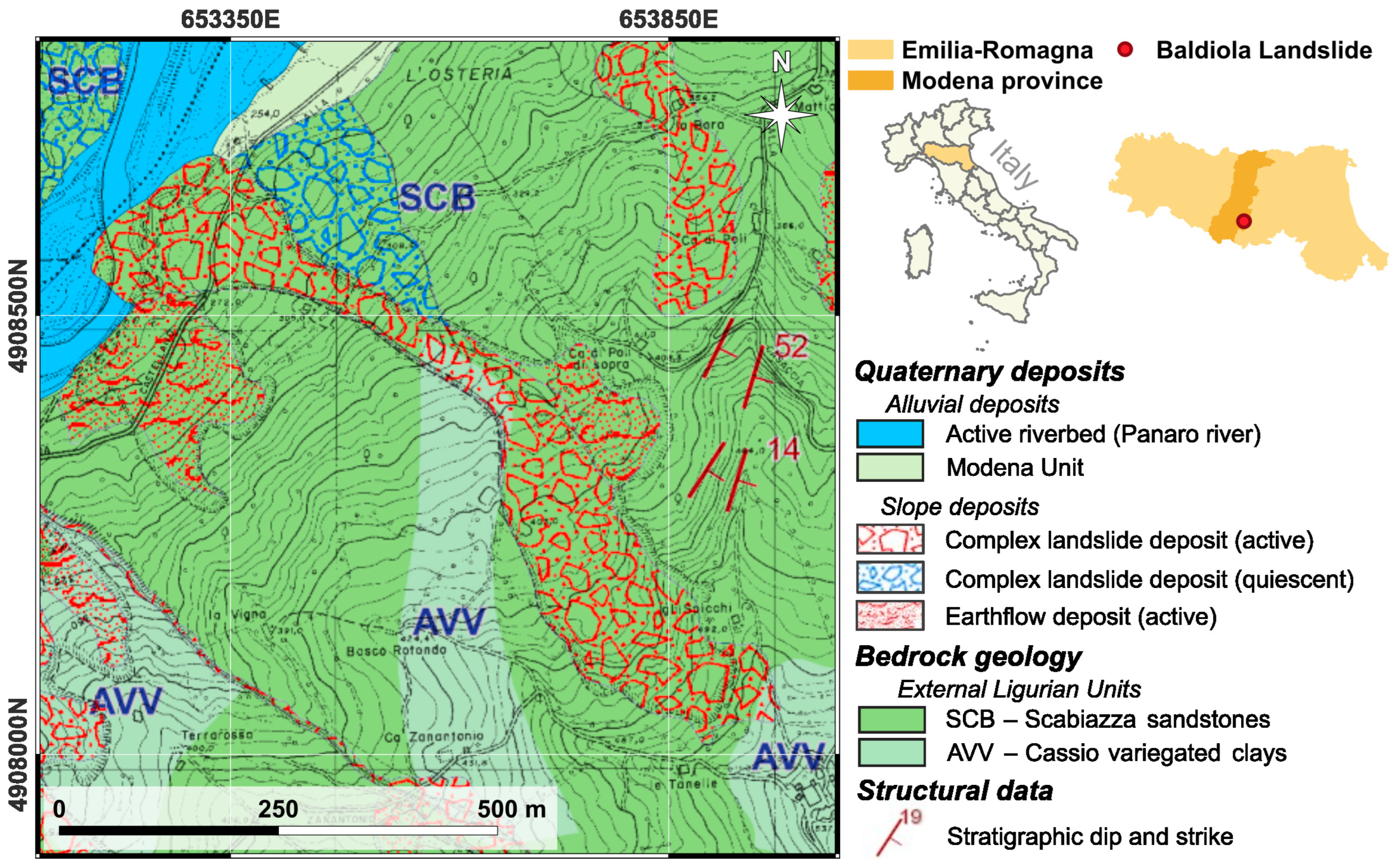
2.1. Geographical and Geological Setting

The Baldiola landslide (44°18′34″N; 10°55′46″E) is located on the eastern bank of the Panaro River, within the municipality of Montese, near the border with the municipalities of Pavullo nel Frignano and Zocca, Province of Modena (Emilia-Romagna Region, Northern Italy). The landslide ranges in elevation from approximately 300 m a.s.l. (at the base) to over 550 m a.s.l. (at the top). The landslide affects clay-rich formations belonging to the basal complexes of the external Ligurian Units (Figure 1). These formations have an oceanic origin and date back to the late Mesozoic, having evolved through several tectonic phases to now outcrop in this area with chaotic, heavily deformed, and degraded structures. According to Sheet 236 (Pavullo nel Frignano) of the Geological Map of Italy [36] and the Emilia-Romagna Region geological WMS database [37], the landslide occurs within the Scabiazza Sandstone Formation, which consists of clay-to-sandstone alternations in varying ratios [38]. Field observations provide insights into the bedrock characteristics. At outcrop scale, intense deformation hinders the recognition of bedding; where visible, stratifications show a dip-slope configuration. The lithological alternation is dominated by clayey units, with an arenite/pelite (A/P) ratio of less than 1. The sandstone layers are less well-represented and appear heavily weathered and degraded, likely as a result of landslide activity. The clay fraction, which also constitutes the main material in the landslide deposit, is pervasive throughout the observed area.

2.2. Geomorphological Features and Historical Activity

The landslide fits the definition of earthflow according to Cruden and Varnes’s classification [39]. The earthflow body has a total planar length of about 1000 m and covers a total area of 0.044 km². It originates from a complex source zone with a maximum width of 135 m, currently affected by minor reactivations. After an initial steep section, the channel bends rightward near a slope break, adapting its path to the surrounding morphology, and then resumes a steeper descent toward the deposition area. Along this stretch, the channel maintains a fairly consistent width of 30–40 m. The toe of the landslide exhibits alternating phases of advancement and erosion within the Panaro riverbed. The historical records from the Emilia Romagna landslide archive [40] and multi-temporal satellite images [41] confirm the existence and activity of the landslide since at least 1976–1978. During this period, the source area experienced a total retrogression of more than 120 m, with 30–50 m occurring only in the last 18 years (i.e., between 2006 and 2024, Figure 2). At the same time, the active toe front has gradually migrated southward—i.e., upstream relative to the river flow—while leaving behind older, more stable deposits. The landslide activity has also triggered smaller-scale instabilities in surrounding sectors, either directly connected or adjacent to the main body.

At present, the ongoing retrogression of the source area poses a potential threat to a group of houses located upslope. In addition, although the toe’s widening into the riverbed does not currently pose a blockage risk, it may affect flow dynamics over time, potentially altering erosion patterns downstream. This could, in turn, destabilize the opposite riverbank, where additional buildings and the SP4 road are located.

3. Materials and Methods

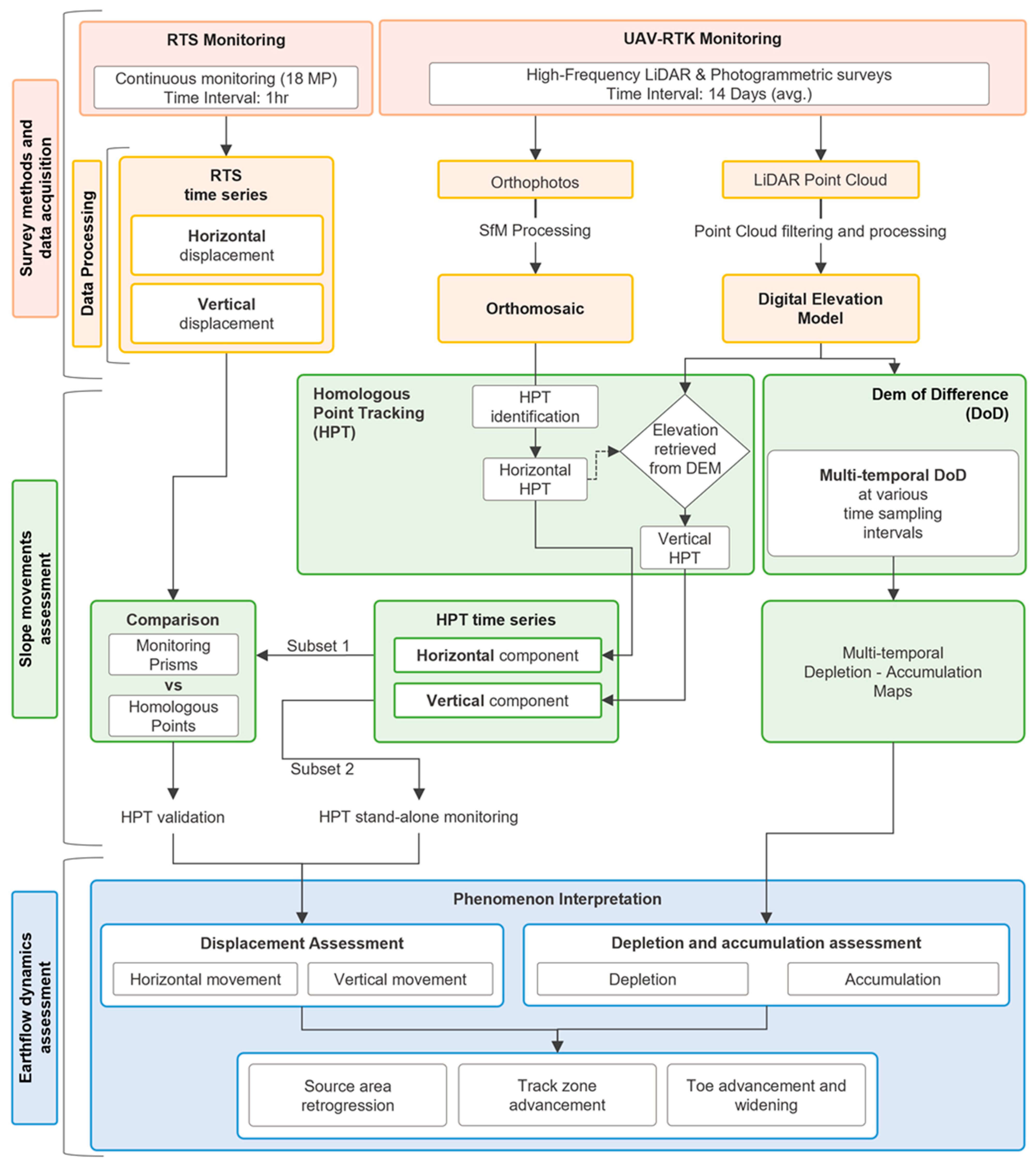
3.1. Operational Framework

A three-phase workflow has been adopted for this study (Figure 3). The first phase focuses on slope surveys, involving both data acquisition and processing. In April 2024, an RTS was installed on site and configured to monitor the displacement of 18 MPs distributed in key locations across the landslide area, ensuring spatial coverage along the entire slope. Simultaneously, high-frequency UAV surveys were conducted, combining photogrammetric and LiDAR acquisitions at average intervals of 14 days, ensuring consistent temporal coverage throughout the monitoring period. UAV data processing includes the generation of high-resolution orthophotos via Structure-from-Motion (SfM) photogrammetry and the creation of Digital Elevation Models (DEMs) from filtered LiDAR point clouds.

The second phase deals with slope movement assessment, including displacement assessment and terrain evolution analysis. RTS data provide direct, high-accuracy measurements, while UAV-derived products support the application of the HPT method, which is applied separately in horizontal and vertical displacement components. Horizontal displacement is estimated by tracking reference features on orthomosaics; vertical displacement is retrieved by extracting elevation values from sequential DEMs at the updated HP locations. HPT is first applied to a subset of 18 HPs located near monitoring prisms (MPs), enabling direct comparison and validation. Once validated, the method is extended to a second subset of four stand-alone HPs. Additionally, multi-temporal DoD analysis is performed to evaluate accumulation and depletion patterns across the slope. DoDs are computed at different time intervals to assess how monitoring frequency influences the interpretation of short-term terrain changes. Although both vertical HPT and DoD are derived from the same DEM dataset, they provide fundamentally different types of information. Recognizing this distinction is essential for correctly interpreting UAV-derived products and understanding the complementary roles of each method in landslide analysis. In fact, despite the frequent association of DoD with vertical displacement, the two quantities are not equivalent (Figure 4). HPT quantifies ground displacement along the trajectory of specific features, providing point-based measurements that are representative of actual surface motion. Conversely, DoD evaluates elevation differences at fixed spatial coordinates, detecting local surface changes—such as accumulation or depletion—without tracking displacing elements.

The third phase addresses earthflow dynamics analysis and focuses on interpreting the processed data to support a comprehensive understanding of landslide behavior. The comparison between RTS and HPT measurements is used to examine displacement, distinguishing between horizontal and vertical components. Additionally, the temporal sequence of DoD maps is analyzed to identify depletion and accumulation patterns across the landslide area and to evaluate slope evolution.

3.2. Survey Methods

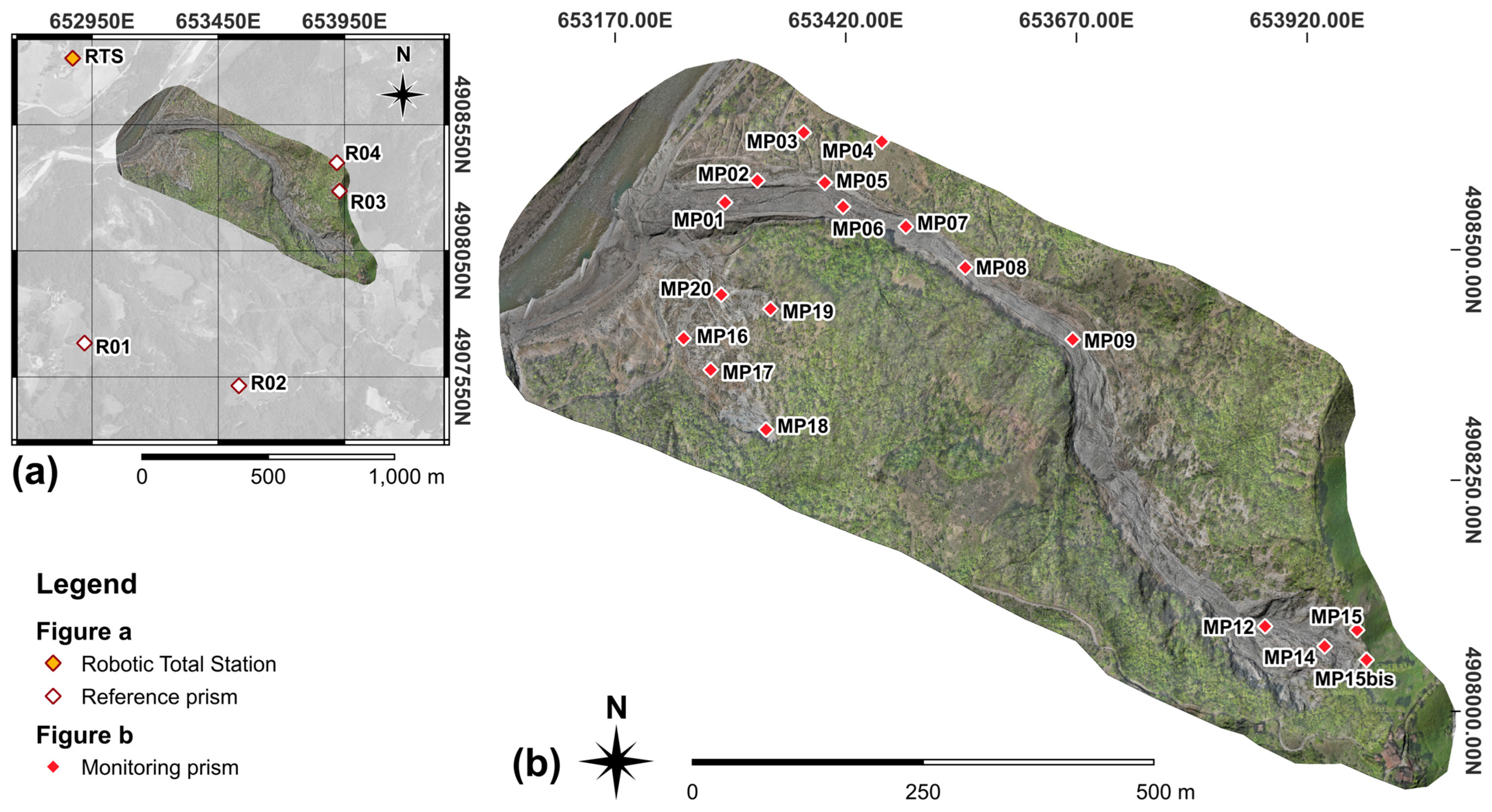
3.2.1. Robotic Total Station Monitoring

RTS monitoring was based on a Trimble S9 robotic total station (Trimble Inc., Westminster, CO, USA), operated in free station mode and based on polar survey geometry. The instrument was configured via Trimble 4D Control (version 6.3.0) software with a one-hour duty cycle and was used to monitor 18 monitoring prisms (MPs) and four fixed reference prisms, which were positioned in stable areas to enable automatic corrections of the instrument position. The RTS was installed on a reinforced concrete base located on the opposite bank of the Panaro River, directly facing the landslide body. A plywood shelter was built to protect the station from direct sunlight and rainfall. The system was powered by the electrical grid and equipped with a backup battery to ensure continuous operation in case of a power outage. MPs were distributed to ensure representative coverage of the landslide: (i) along the active track zone; (ii) in previously active but now abandoned unstable areas; (iii) in the source area; and (iv) over portions of the slope near the main landslide body affected by instability. The position of the monitoring prisms along the slope is shown in Figure 5.

Between April and August 2024, RTS monitoring has provided both horizontal and vertical displacement data for each MP. To georeference the RTS and ensure consistency with UAV-derived datasets, the flight area of one survey was extended to include the RTS installation, allowing its position to be identified. Monitoring was carried out continuously throughout the observation period, except for a temporary interruption between 23 May and 4 June 2024 due to a connection issue. Minor interruptions affecting individual MPs were caused by landslide-related displacements or rotations; affected prisms were replaced as soon as possible to restore measurements.

3.2.2. UAV Monitoring

UAV monitoring was based on a DJI Matrice 350 RTK with a DJI Zenmuse L2 LiDAR scanner as the onboard payload (DJI Technology Co., Ltd., Shenzhen, China). The device features an integrated dual-frequency RTK GNSS receiver for high-precision positioning and operates in connection with a local GNSS reference station (DJI D-RTK 2 Mobile Station, DJI Technology Co., Ltd., Shenzhen, China) to enable RTK corrections. From April to August 2024, a total of 10 UAV surveys were conducted over an area of 0.46 km², with average time intervals of 14 days between surveys (min 4 to max 22 days, see

Table 1. List of the 10 UAV surveys conducted in the period between 12 April and 7 August 2024.

UAV Surveys
Survey	Date (DD MM YYYY)	Time Interval (Days)
1	12 April 2024	-
2	29 April 2024	17
3	3 May 2024	4
4	10 May 2024	7
5	23 May 2024	13
6	30 May 2024	7
7	7 June 2024	8
8	27 June 2024	20
9	16 July 2024	19
10	7 August 2024	22

, with variations driven by weather conditions or increased landslide activity requiring shorter revisiting times).

Flight parameters were kept consistent, following a pre-programmed flight plan to ensure data repeatability (

Table 2. Summary of flight, LiDAR, and photo sampling parameters used for mapping operations.

Fight Parameters
Flight mode	Planned Route
Mapping area	0.46 km2
Flight altitude	100–120 m
Altitude mode	“Terrain follow”
Speed (m/s)	4–6 m/s
LiDAR Parameters
Expected Point Cloud Density (avg.)	130–140 points/m2
Final Point Cloud Density (avg.)	~500 points/m2
LiDAR Side Overlap	30–40%
Return mode (n° returns)	5
Photo Sampling Parameters
Photo Side Overlap	45%
Photo Forward Overlap	70%
Range of N° of photos per survey	Min 175–Max 227

). Minimal adjustments to flight altitude and speed were applied to account for environmental variations, such as temperature, wind, and seasonal changes in vegetation cover. For instance, increased vegetation density during summer requires a lower flight speed to enhance ground detection accuracy, while lower temperatures in late winter and early spring require higher speeds to optimize battery efficiency and flight endurance. These modifications, though limited, are necessary to maintain data quality and survey consistency while ensuring operational safety under varying environmental conditions [42].

During surveys, the DJI D-RTK 2 antenna was positioned in a fixed benchmark using a DJI D-RTK 2 Base Tripod Station, which ensured levelling and a constant height of the RTK antenna thanks to the fixed-length rod. The benchmark consisted of a 20 mm iron bar fixed with chemicals to the concrete raft foundation of the RTS pillar. The decision to use the DJI D-RTK 2 antenna rather than NRTK (Network Real Time Kinematics) services was based on the fact that it brings significant benefits for the spatial alignment of successive surveys, improving the repeatability (and thus the precision) of multitemporal comparisons. Specifically, using the DJI D-RTK 2 antenna enabled us to enter fixed coordinates into the RTK antenna in the DJI Terra software (Version 4.3.0; DJI Technology Co., Ltd.: Shenzhen, China), an option that is not available when using NRTK services. In fact, with NRTK services, the coordinates of the reference point (generated by integrating the multitemporal surveys within a network of permanent stations) may change from one survey to another, causing variations in the georeferencing of the DEMs.

The positional stability of the DJI D-RTK 2 benchmark and the RTS pillar over time was verified in different ways, all of which indicate only a seasonal hysteresis in the range of ±2 cm (Figure 6). The first verification method involved repeating the static GNSS survey of the benchmark and RTS pillar at the times of UAV surveys 1, 5, and 10. This allowed referencing of the benchmark to the UTM coordinate system with the WGS84 datum, projected in zone 32N (EPSG:32632). Furthermore, since the RTS pillar and the DJI D-RTK 2 benchmark share the same raft concrete foundation, the RTS coordinates over time (calculated in the free-station mode) are a reliable proxy of the stability of these points. A scatter plot and time series of easting and northing of the RTS coordinates calculated in the RTS free-station surveys from May 2024 to July 2025 are presented in Figure 6a,b. Both indicate that the RTS is stable with a seasonal hysteresis in the range of ±2cm. Finally, indirect evidence of the stability of the RTK reference point coordinates is provided by the degree to which repeated measures produce the same result (i.e., precision) for man-made structures located along the riverbed, outside the influence of landside movements (Figure 6c). Different UAV surveys indicate that their position is unchanged at the sub-pixel scale (Figure 6d,e), demonstrating that DEMs are not affected by spatial drifts over time.

The DJI L2 sensor was set up for the simultaneous acquisition of both LiDAR data and orthophotos (Table 2). All LiDAR and photographic acquisitions were performed from a nadir position. Given the expected presence of vegetation, the LiDAR sensor was configured to record in “penta-return mode” (i.e., five returns recorded, maximum available) to improve ground detection. The overlap of the laser scanner acquisition was set between 30% and 40%, depending on survey needs.

Photographic acquisition, primarily for color sampling and point cloud coloring, was intentionally oversampled, with 40% side overlap and 70–80% forward overlap, to ensure the collection of a sufficient number of images to generate high-resolution orthomosaics as a secondary product, processed separately from the LiDAR data.

The datasets acquired through UAV surveys, consisting of LiDAR point clouds with an average density of 500 points/m² and an orthophoto archive containing a minimum of 175 images per survey, were processed using DJI Terra software (DJI Technology Co., Ltd. Version 4.3.0, [43]). Point clouds were used to generate Digital Elevation Models (DEMs), following the software’s optimized settings (

Table 3. DJI Terra setting parameters for point cloud and orthomosaic processing.

Point Cloud Processing: DJI Terra Setting Parameters
Point Cloud Density selection	By percentage (100%)
Ground Type	“Gentle Slope”
Building max diagonal	20 m
Iteration angle	6°
Iteration distance	0.5 m
DEM output resolution (GSD)	25 cm/px
Orthomosaic Processing: DJI Terra Setting Parameters
Resolution (High-Medium-Low)	High
Computation method	Standalone Computation
Light Uniformity	If necessary
Ground Sampling Distance: Min-Max (Avg)	2.95–4.32 (3.23) cm/px

). The processing workflow, based on the analysis of spatial relationships such as angles and distances, distinguishes ground points from non-ground elements and includes the filtering of vegetation and anthropic elements to extract a clean terrain representation.

DJI Terra software enables the manual selection of the output Ground Sampling Distance (GSD), ranging from a minimum of 5 cm/px. For this study, three different GSD values were tested: 5 cm/px, 15 cm/px, and 25 cm/px. A comparative analysis (Figure 7) revealed that low GSD values, particularly 5 cm/px, lead to increased fragmentation and noise, especially in vegetated areas where LiDAR penetration is limited during late spring and summer. The 25 cm/px resolution effectively minimizes these effects, preserving a stable and continuous surface representation while maintaining sufficient detail for landslide analysis. Additionally, it provides an appropriate trade-off between filtering out noise and preserving elevation accuracy, avoiding over-fragmentation while retaining reliable vertical displacement data. The 25 cm/px resolution was selected as the optimal trade-off between surface detail and noise reduction. The impact of this choice on the accuracy of DoD calculation is beneficial, since the use of DEMs with lesser noise rules out several artefacts from the DoD computation that are mostly located in critical areas such as fracture zones in the source region (see Figure 7d–f). Also, the accuracy of DoD calculations is mostly affected by the absolute vertical accuracy of surveys, related to RTK corrections rather than pixel size, so that reducing the resolution does not necessarily affect the accuracy of differential calculations.

The UAV photographic dataset was processed separately using DJI Terra software (Table 3). Orthomosaics with a final Ground Sampling Distance (GSD) ranging from 2.95 to 4.32 cm/px (average 3.23 cm/px) have been produced and used to track HP points. Such a narrow range of variation in resolution has no substantial impact on the identification over time of HPs’ positions. All products were compared in a GIS environment [44], confirming a consistent planimetric alignment across all UAV surveys and vertical discrepancies—assessed over assumed stable areas—consistently below 10 cm.

3.3. Slope Movements Assessment

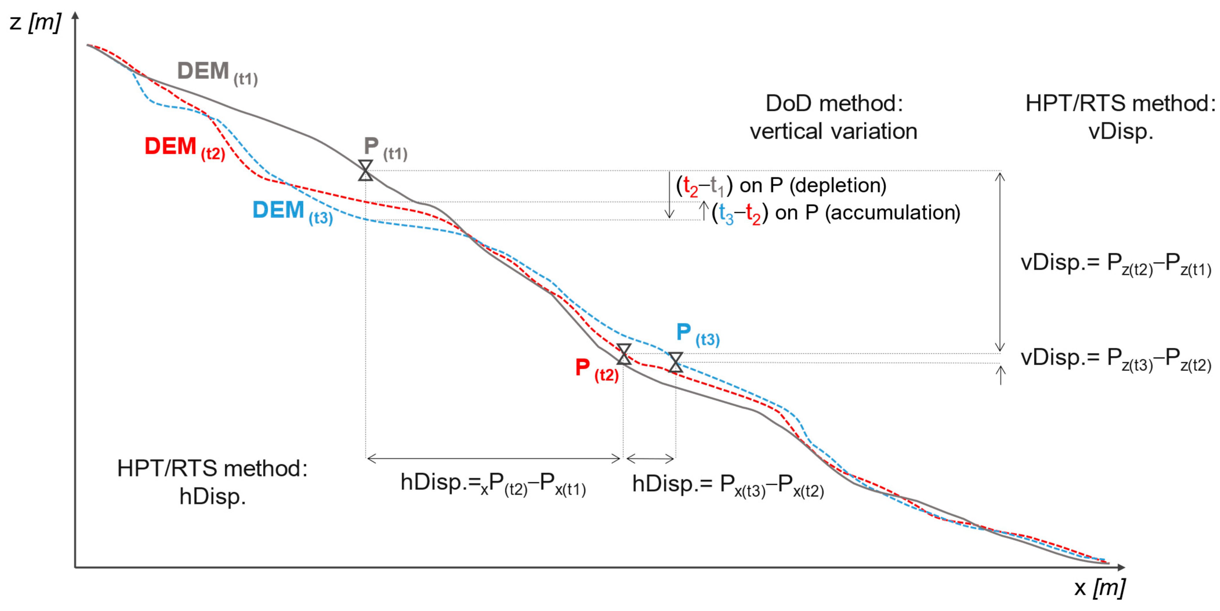
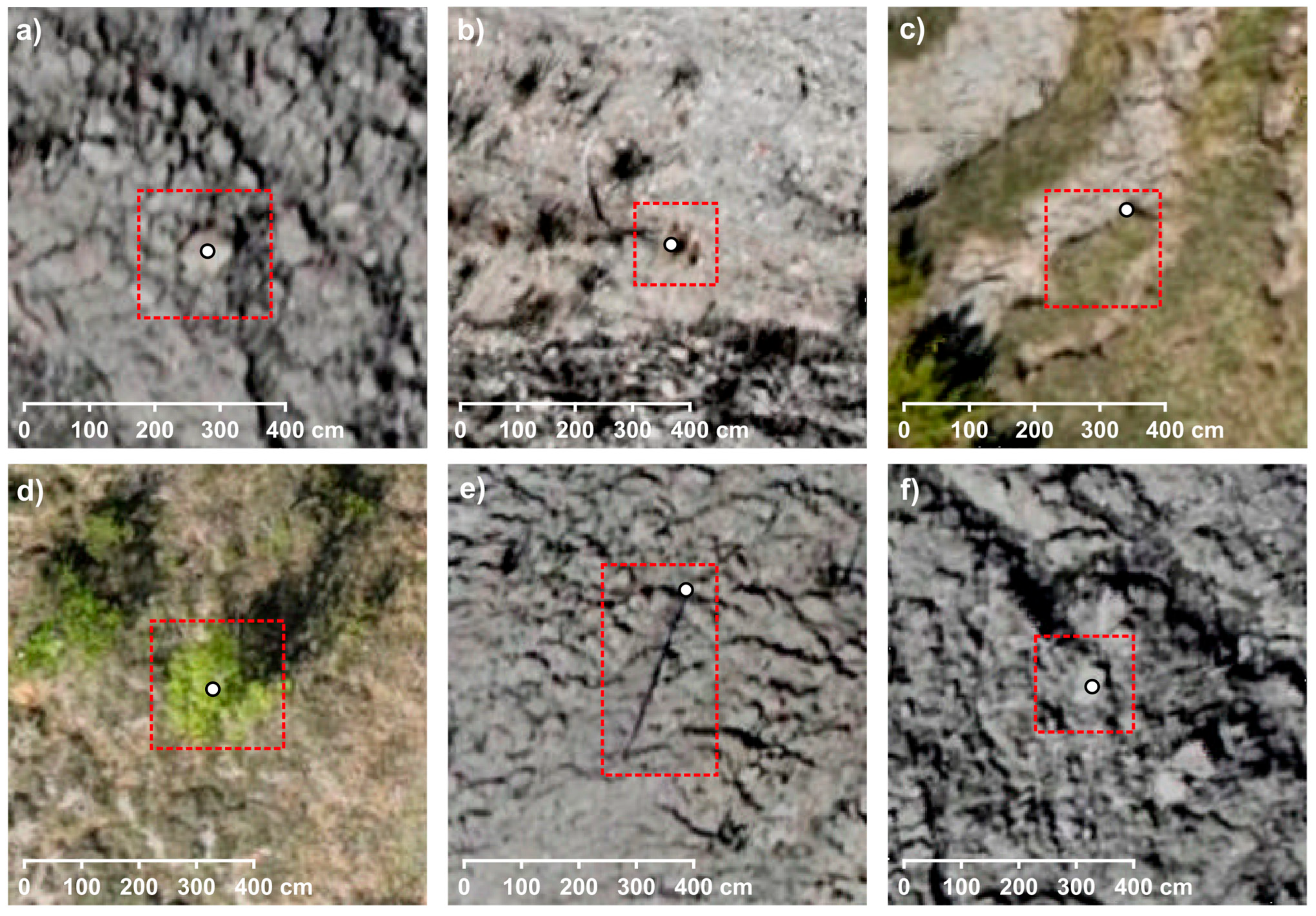
3.3.1. Horizontal and Vertical Displacement Assessment with Homologous Point Tracking

DEMs and orthomosaics derived from UAV surveys have been used to assess displacement through the homologous point tracking method. HPT is a displacement measurement technique based on the manual identification and tracking of natural surface elements that remain clearly identifiable across consecutive surveys. These elements, referred to in this study as Homologous Points (HPs), are natural objects or morphological features already present on the slope—such as isolated rocks, vegetation clusters, or soil patches—that can be recognized over time and are assumed to be physically integrated with the terrain surface. Under this assumption, HPs are considered kinematically coherent with the surrounding ground, and their displacement is interpreted as representative of local surface movement.

In this study, a total of 22 HPs were selected through the observation of UAV-derived orthomosaics. A first subset, consisting of 18 HPs, was deliberately selected in proximity to the MPs to enable a direct comparison between the two techniques. This enables the validation of UAV-based displacement measurements by assessing their consistency with RTS-derived data. A second subset, consisting of four additional HPs, is selected in locations not related to MPs’ positions. Given the specific conditions of this case study, where the RTS position does not allow monitoring of a certain sector of the landslide, these HPs are placed in areas of the landslide not covered by RTS monitoring, in order to include otherwise unmonitored parts of the landslide (Figure 8).

The objects and terrain features selected as HPs include boulders and rock blocks of various sizes and shapes, soil patches and clumps that maintain a recognizable form during movement, and vegetative elements such as shrubs, small bushes, tree trunks, and large branches. The selection aims to maximize tracking reliability by choosing objects that remained stable and identifiable over time. Figure 9 illustrates some representative examples.

Details for each HP, including object type, dimensions, and distance to the corresponding MP, are provided in

Table 4. HPs’ main characteristics, dimensions, and functions.

HP	Subset	Object	Size (Reference Dimension)	Tracking Point Position	Distance from the Corresponding MP (12 April 2024)
HP01	1	Rock block	0.47 m (max. diameter)	Centroid	5.61 m
HP02	1	Shrub	0.45 m (diameter)	Centroid	3.94 m
HP03	1	Shrub/ little tree	1.65 m (diameter)	Centroid	2.92 m
HP04	1	Shrub	1.19 m (diameter)	Centroid	15.39 m
HP05	1	Shrub	0.54 m (diameter)	Centroid	2.81 m
HP06	1	Downed branch	0.13 m (branch diameter)	Fixed branch end	9.74 m
HP07	1	Rock block	0.49 m (max. length)	Fixed rock edge	8.40 m
HP08	1	Downed trunk	0.30 m (trunk diameter)	Fixed trunk end	20.45 m
HP09	1	Downed tree body	0.34 m (main trunk diameter)	Main trunk end	11.22 m
HP12	1	Rock block	0.80 m (max. length)	Centroid	1.07 m
HP14	1	Rock block	0.24 m (diameter)	Centroid	0.92 m
HP15	1	Bare ground patch/rock block	0.20 m (max. length)	Centroid	3.09 m
HP15bis	1	Shrub/grass clump	0.28 m (max. length)	Centroid	2.15 m
HP16	1	Rock block	0.83 m (max. length)	Fixed rock edge	12.10 m
HP17	1	Rock block	0.70 (diameter)	Centroid	11.73 m
HP18	1	Shrub	0.97 m (diameter)	Centroid	12.13 m
HP19	1	Ground patch	0.58 m (width)	Fixed edge	3.82 m
HP20	1	Shrub	0.75 m (diameter)	Centroid	0.59 m
HP01h	2	Shrub	0. 51 m (diameter)	Centroid	-
HP02h	2	Rock block	0.44 m (diagonal)	Centroid	-
HP03h	2	Downed branch	0.19 m (branch diameter)	Fixed branch end	-
HP04h	2	Rock block	0.67 m (diagonal)	Centroid	-

. The recorded dimensions represent the most relevant dimension for tracking purposes, depending on the type and geometry of the object. For rock elements, either the maximum length or diameter was measured, based on whether the reference point was set on an edge or at the centroid. For vegetative elements such as bushes and branches, the canopy or stem diameter was recorded, as it defines their visible footprint. For soil patches and turf clumps, the widest dimension was used, since it best represents their overall extent and interaction with the surrounding flow.

Horizontal displacement was assessed by visually tracking the planar position of each HP across the orthomosaics sequence. The tracking was carried out sequentially, starting from the first acquisition and continuing through all subsequent surveys. For each HP, updated positions were recorded at every step, and horizontal displacement was calculated by measuring the planar distance between successive HP positions (Figure 10a,b). To ensure reliable tracking, the selection of HPs follows the fundamental criterion of visual continuity: objects or terrain features must remain identifiable throughout the UAV survey sequence, allowing consistent displacement measurements over time. Minor temporary interruptions in tracking are tolerated only if the point can be reliably relocated and no better alternative is available. Furthermore, for HPs selected to validate UAV-based monitoring, two additional criteria were considered: their proximity to MPs, to facilitate direct spatial comparison, and their location within the same kinematic sector of the landslide, to ensure that HPs and corresponding MPs are subject to similar displacement patterns.

Vertical displacement is derived by associating the HP with the elevation at its updated position by using sequential 25 cm/px DEMs. This procedure was repeated for each acquisition, generating a time series of elevation values for each HP. Vertical displacement was computed by extracting elevation values at the updated HP positions from each DEM in the sequence, and calculating their variation over time. This approach allows for a progressive reconstruction of surface elevation changes throughout the monitoring period (Figure 10c). The vertical analysis was therefore conducted directly on DEMs but strictly relies on horizontal HPT to ensure spatial and temporal coherence across the dataset. This guarantees that elevation changes reflect real vertical displacement rather than independent terrain variations.

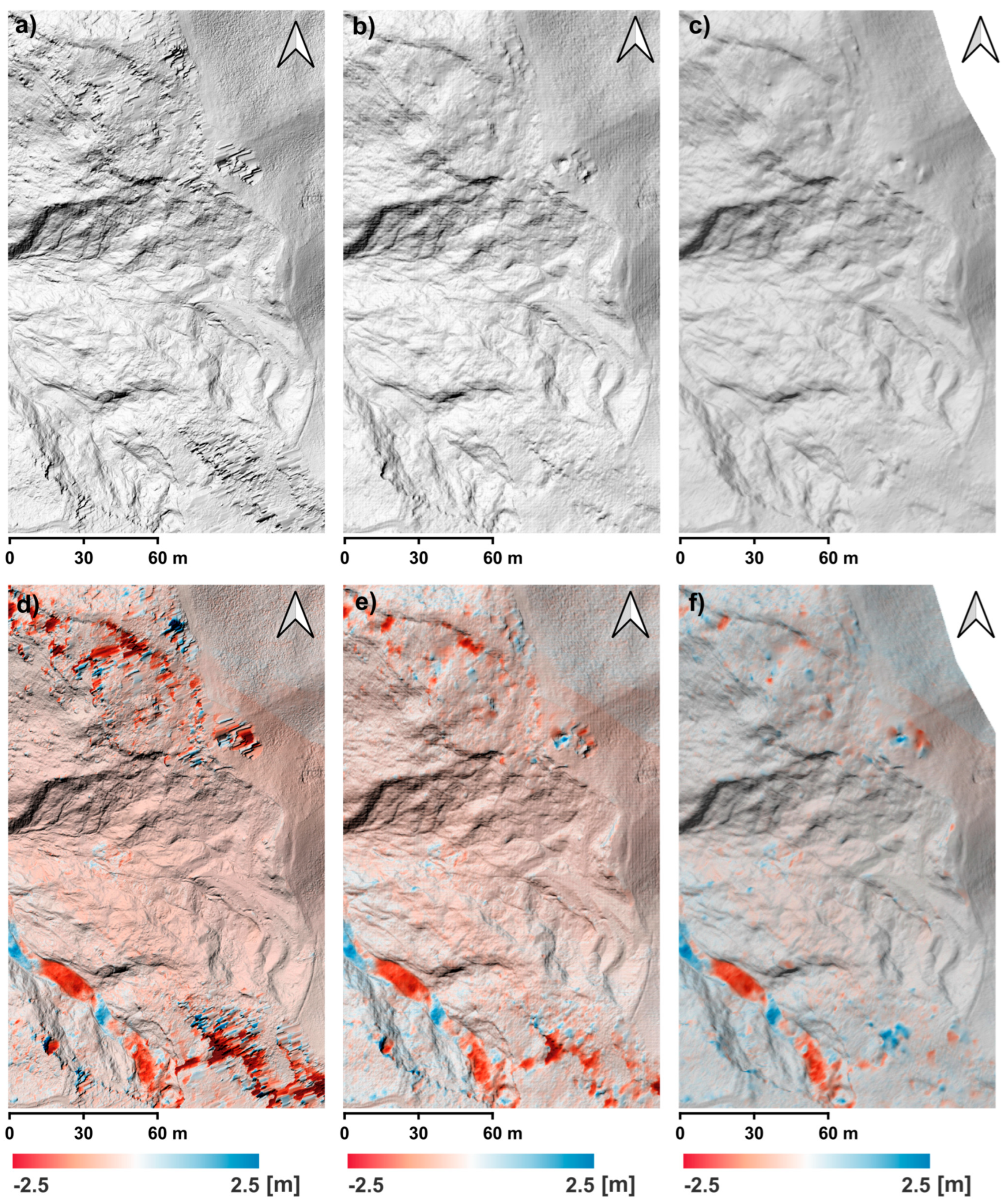
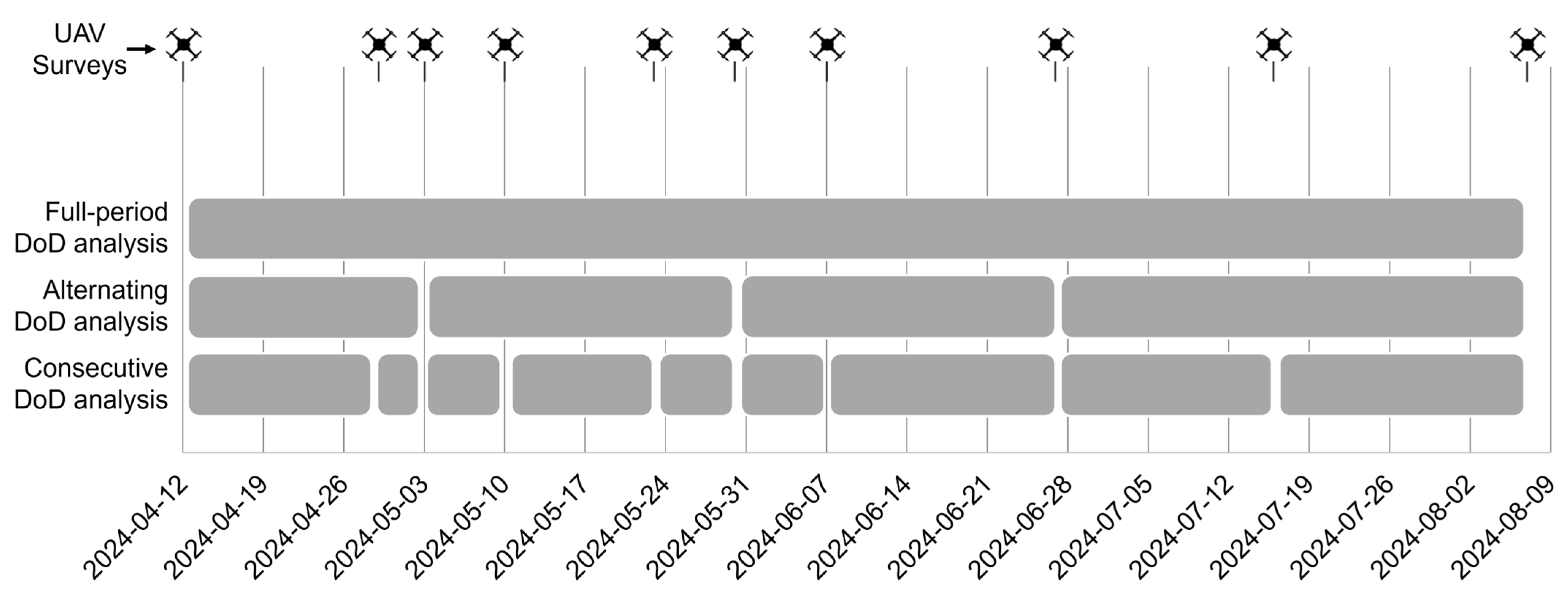
3.3.2. Analysis of Depletion and Accumulation Using Multi-Temporal DoD

DEM of Difference (DoD) analysis was used to assess depletion and accumulation processes over time by comparing sequential DEMs. The DoD was computed by subtracting, for each pixel, the elevation values of a DEM acquired at an earlier time from those of a DEM obtained at a later time. Specifically, negative values indicate depletion, corresponding to material displacement or removal, whereas positive values indicate accumulation, representing areas where material has been deposited.

In this study, DoD analysis leveraged 25 cm/px DEMs and was performed using multiple temporal intervals. In particular, three temporal sampling strategies were adopted: (i) a consecutive approach, computing DoDs between each UAV survey and the next; (ii) an alternating approach, comparing non-consecutive surveys to evaluate broader time spans; and (iii) a full-period approach, comparing the first and last DEMs of the monitoring period. The adopted temporal sampling intervals are shown in Figure 11. Rather than treating each DoD as a stand-alone product, the whole sequence of DoD maps was interpreted to track the spatial evolution of depletion and accumulation patterns throughout the monitoring period.

4. Results

4.1. Spatial Synopsis of HPT and RTS Monitoring Results

Maps showing cumulative planar displacements derived by HPT and RTS monitoring from 12 April to 7 August 2024 are presented in Figure 12. A total of 13 HPs exhibit displacements exceeding 0.5 m, consistently identifying the most active sectors, while the remaining HPs were located in relatively more stable sectors of the landslide. This reveals a marked kinematic heterogeneity within the landslide body. The most active sectors correspond to the mid and lower portions of the earthflow track zone, where several HPs show the highest cumulative displacements. At the same time, more limited displacements were recorded in the source area.

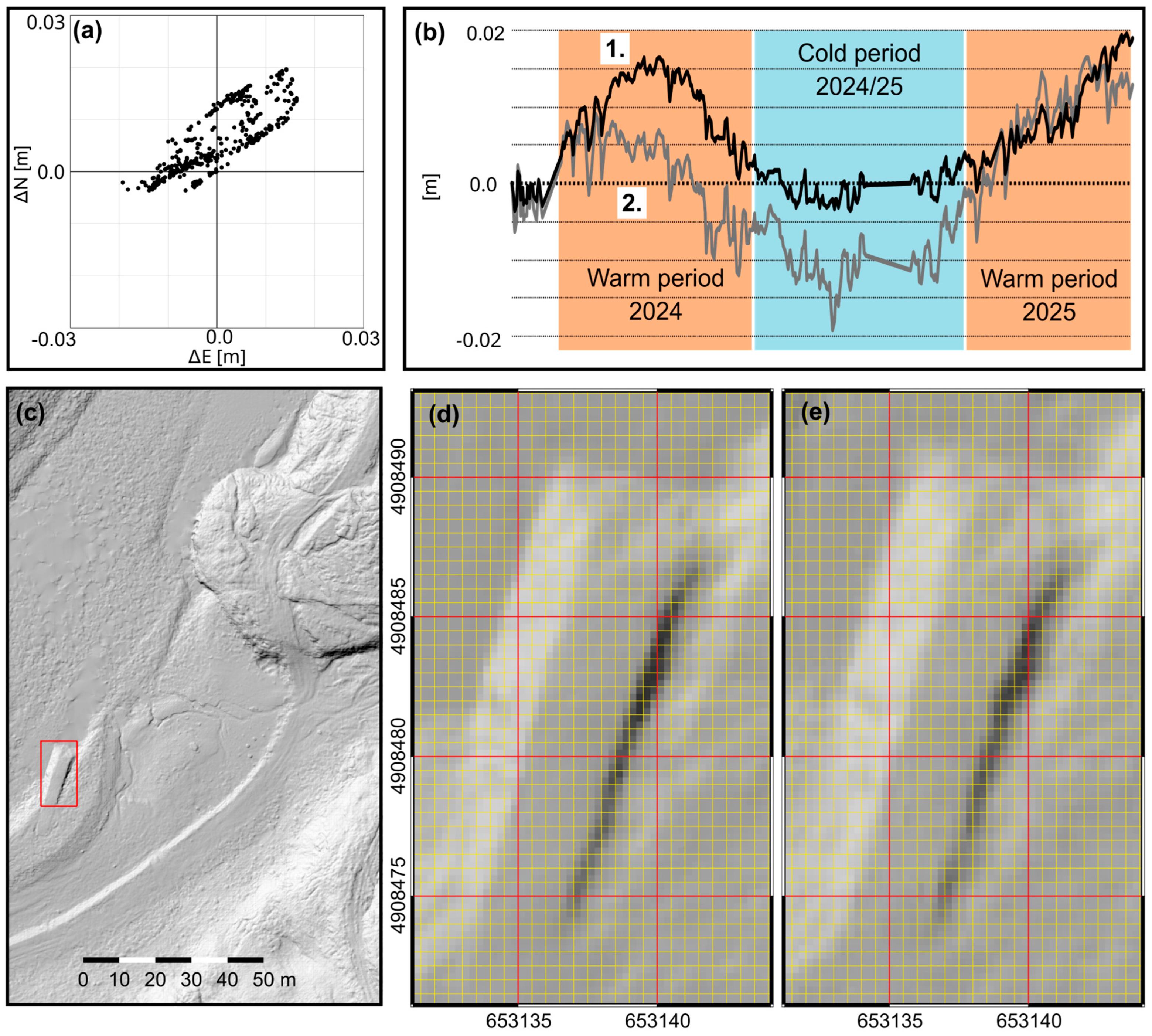
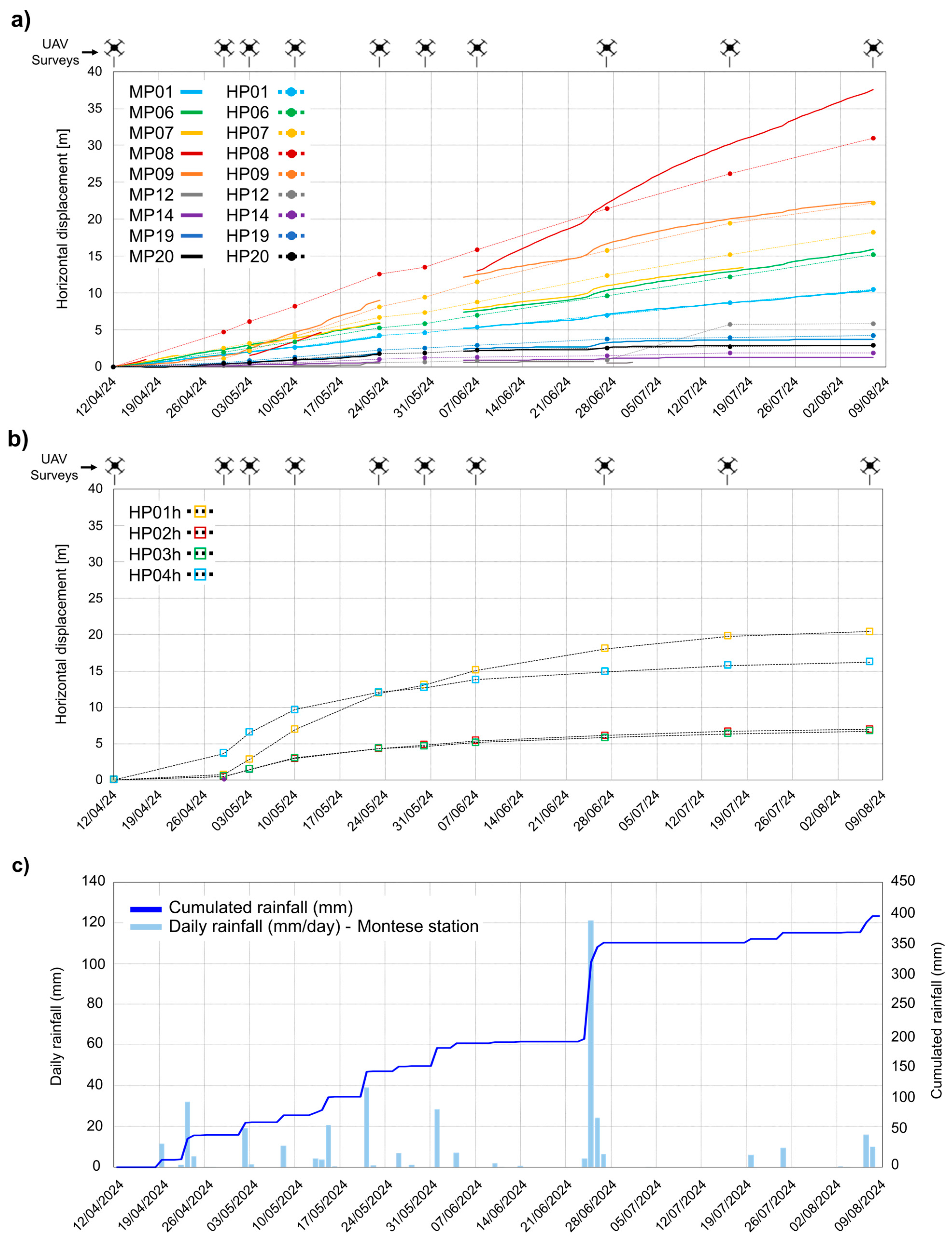
4.1.1. Time Series of HPT and RTS Horizontal Displacements

The comparison between the time series of HPT and RTS horizontal displacements is presented in Figure 13.

For HPs located near RTS-monitored prisms (subset 1, Figure 13a), the MP08–HP08 pair exhibits the highest measured displacement, with RTS values reaching up to 40 m and HPT values slightly lower (~30 m). While initial displacements are overestimated by HPT, a progressive underestimation occurs later in the monitoring period, resulting in a final discrepancy of approximately 6 m. The reason for the large discrepancy between MP08 and HP08 is that they are located in a very active portion of the landslide, and they are not sufficiently close to one another. Consequently, they are progressively affected by different movement rates as the landslide evolves to a total cumulative displacement of approximately 40 m.

Conversely, the MP09–HP09 pair exhibits excellent agreement between the two techniques, with cumulative displacements ranging from 20 to 25 m and a consistent trend throughout the monitoring period. Similarly, a good fit is observed for the MP06–HP06 and MP07–HP07 pairs, with displacements ranging from 15 to 20 m. MP06–HP06 shows nearly identical displacement values across both methods, while MP07–HP07 exhibits a minor overestimation in HPT results, limited to 1–2 m. The MP01–HP01 pair, located in the lower track zone, displays a cumulative displacement of approximately 10 m with an almost perfect match between methods. In the source area and the upper unstable sector near the landslide toe, smaller displacements are recorded. For instance, MP12–HP12 and MP14–HP14 report movements below 5 m, with a strong agreement between RTS and HPT. Similar displacement magnitudes and matching trends are also observed for MP19–HP19 and MP20–HP20, both of which are located in the active portion of the unstable zone upstream of the toe.

For HPs not located close to RTS (subset 2, Figure 13b), HP02h and HP03h exhibit comparable displacement trends, characterized by steady and continuous movement throughout the monitoring period, with cumulative values ranging from 5 to 10 m. HP01h and HP04h follow similar trajectories, although HP04h shows an earlier acceleration phase, whereas HP01h reaches slightly higher final displacement values. By the end of the observation period, HP01h approaches 20 m, while HP04h ranges from 15 to 18 m. Although no RTS data are available for this sector, the recorded trajectories confirm ongoing material displacement within this portion of the landslide body.

During the monitoring period, the landslide site experienced a total cumulated rainfall of 396 mm, related to a dozen rainfall events, lasting from one to four days, reaching a maximum intensity of 120 mm/day (Figure 13c). The relationships between movement patterns and rainfall are presented in the discussion section.

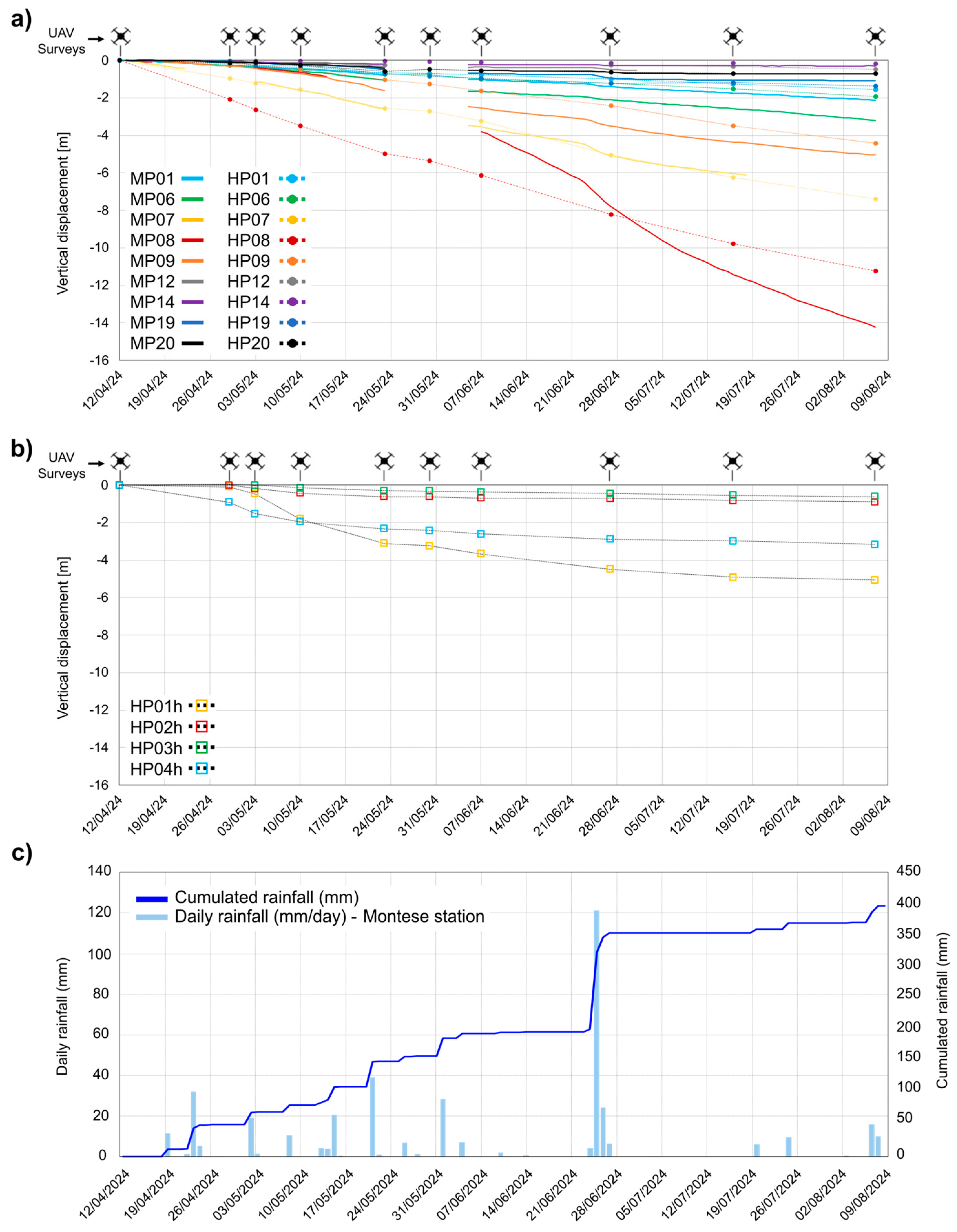
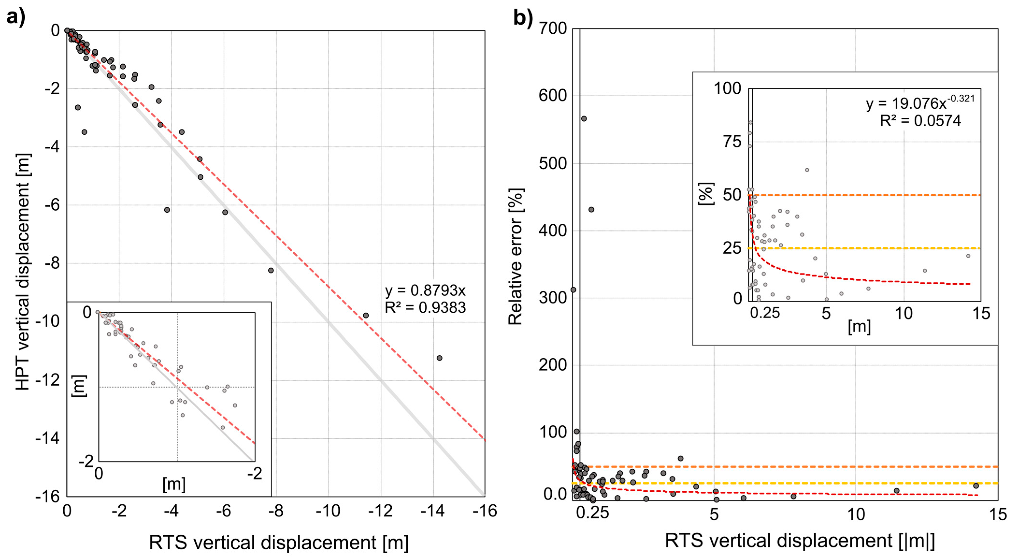
4.1.2. Time Series of HPT and RTS Vertical Displacements

A comparison between the time series of HPT and RTS horizontal displacements is presented in Figure 14. The vertical displacement patterns reflect the typical behavior of an earthflow, with a general lowering of points along the downslope direction. Elevation loss is consistent with the local topography and the magnitude of horizontal displacement. For HPs located near RTS-monitored prisms (subset 1, Figure 14a), the MP08–HP08 pair exhibits the highest vertical displacement, with HPT values exceeding 11 m and RTS surpassing 14 m. The temporal trends are similar, although HPT overestimates movement in the initial phase and progressively underestimates it after late June. HPT data follow a near-linear progression, while RTS captures a clear acceleration phase between 21 and 28 June. The MP07–HP07 pair records approximately 8 m of vertical displacement via HPT, with RTS data (available until 18 July), showing an almost identical evolution. MP09–HP09 also shows strong agreement, with HPT slightly underestimating total displacement. A similar pattern is observed in MP06–HP06, where RTS measures around 3 m and HPT remains below 2 m. The MP01–HP01 pair exhibits a vertical displacement of approximately 2 m, with consistent alignment between both methods throughout the monitoring period. The remaining Subset 1 points (HP12, HP14, HP19, HP20) show displacements equal to or below 2 m. All exhibit coherent trends across methods. In particular, HP12 displays a marked acceleration between 27 June and 16 July, coinciding with the interruption of RTS data at MP12 on 2 June.

For HPs not located close to RTS (subset 2, Figure 14b), the vertical trends are similar to those observed in the horizontal component. HP02h and HP03h follow nearly identical trajectories, each reaching about 1 m of displacement. HP01h and HP04h experience larger vertical displacements, ranging from 3 to 6 m. A clear acceleration phase is observed between late April and early May, first in HP04h and subsequently in HP01h, which ultimately records the highest values within the group.

These movements occurred in response to the rainfall pattern presented in Figure 14c (same as Figure 13c).

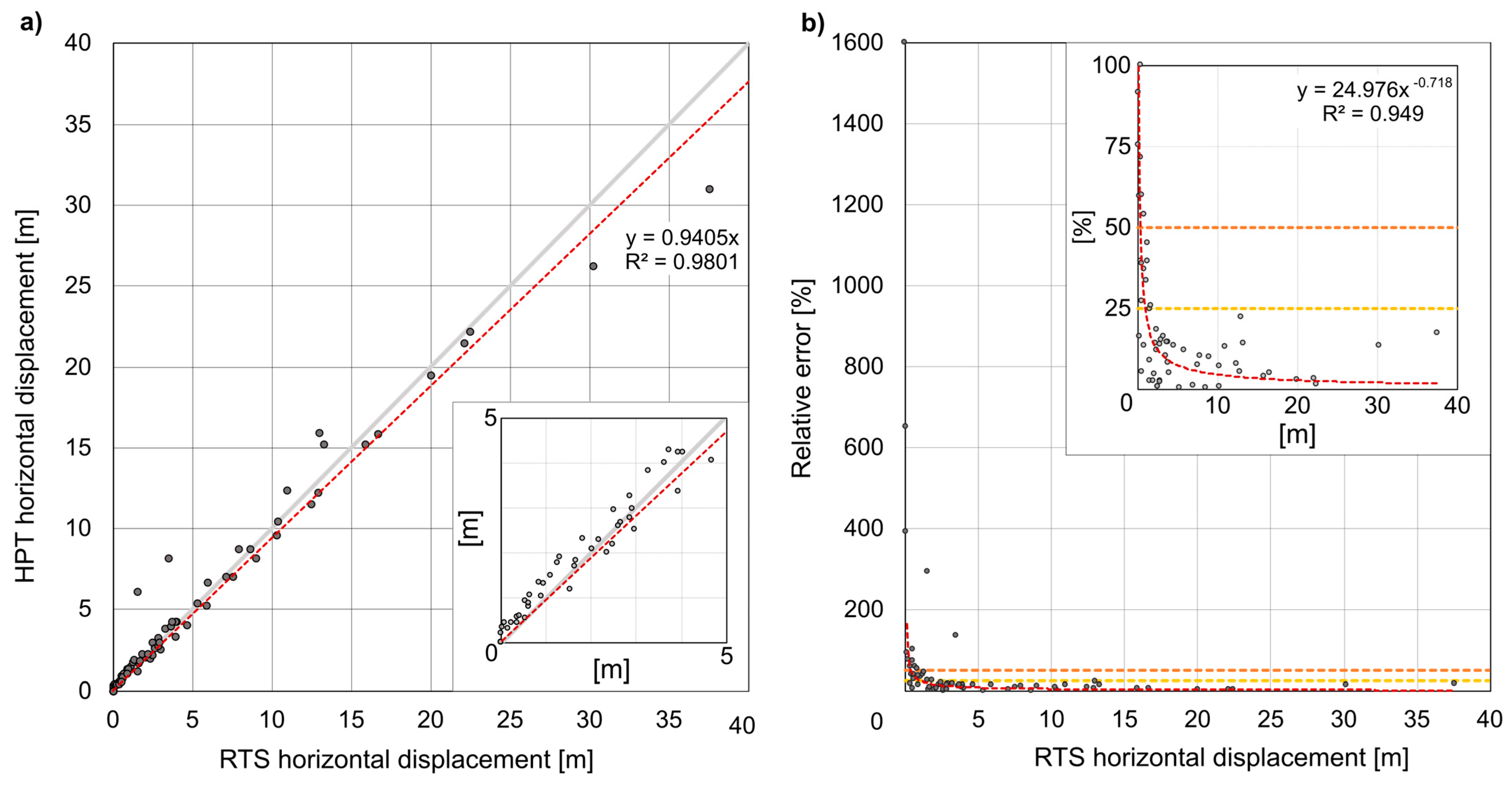
4.1.3. Correlation Between HPT and RTS Displacement Data

The correlation between HPT and RTS displacement data validates the UAV-derived results. Results are presented in Figure 15 and Figure 16, which, respectively, refer to a point-by-point comparison of horizontal and vertical displacements accumulated between 12 April and 7 August 2024. In both cases, panel (a) displays a scatterplot of RTS versus HPT measurements, while panel (b) shows the relative error as a function of RTS-derived displacement. Notably, both the planar and the vertical components indicate the tendency of HPT to underestimate displacement compared to RTS.

For the horizontal displacement, the linear fit exhibits a slope of 0.94, and an R² value of 0.98 confirms a strong alignment between the datasets (Figure 15a). The vertical displacement comparison also shows good agreement, with a slope of 0.88 and an R² of 0.94 (Figure 16a). The relative error distribution exhibits a power-law trend with a rather good fit for planar displacements (R² = 0.95) (Figure 15b), and a much poorer fit for vertical displacements (R² = 0.06) (Figure 16b). On this basis, in the planimetric component, a 25% relative error corresponds to 0.99 m and a 50% relative error corresponds to 0.38 m. Due to the poor fit, it is not possible to provide a robust estimate of the displacements associated with the same relative percentages for the vertical component. Notably, in our case study, almost all of the calculated HPs planar displacements between subsequent surveys are higher than the values associated with a 50% relative error, which can be considered an acceptability threshold. On this basis, the precision of the method can be considered appropriate for planar displacements larger than 40 cm between subsequent surveys. This indicates that the adopted approach might not be suitable for landslides exhibiting displacement rates lower than those characterizing our landslide.

The correlation between RTS and HPT displacement data confirms a high level of overall agreement in both horizontal and vertical components. The correlation values obtained are extremely high, with minimal divergence between the two methods across most monitored HP–MP pairs. These results highlight the capacity of HPT to reproduce displacement trends consistent with those obtained through high-precision ground-based measurements. However, a few discrepancies between RTS and HPT can be observed, which are due to different reasons. First, although HPs are selected to ensure maximum comparability with the RTS prisms, it must be noted that measurements are related to physically distinct objects. RTS tracks optical prisms mounted on rigid supports elevated from the ground, while HPT follows natural surface features that, although carefully chosen to correspond spatially, remain separate from the MPs. In a deforming system such as an earthflow, characterized by plastic and heterogeneous movement over time, even minimal spatial offsets can lead to measurable differences in displacement magnitude. An additional element to consider is that MPs are installed on 1.8 m long iron bars driven into the ground to a depth of 1 m. Therefore, their tilting, caused by landslide movements, might result in over- or underestimates of RTS displacements in the range of cm to dm. Conversely, HPT tracks surface-integrated elements that may respond differently due to local constraints or resistances (e.g., roughness or minor surface anchoring). While such effects may appear negligible, over the whole monitoring period, they can result in differences of several centimeters.

Given these factors, the point-based measurement of displacement in a system as complex as an earthflow, which moves several centimeters to meters, inherently involves sources of uncertainty. In the context of active earthflows moving up to moderate rates, achieving sub-centimeter precision is neither a realistic nor (probably) a necessary objective. However, it might be a necessity in other case studies characterized by much slower movements, which consequently require different survey approaches and the adoption of ground control points. What emerges as most relevant in this study is the ability to detect consistent displacement patterns. In all monitored sectors, the drone-derived HPT approach reproduced the same trends in displacement magnitude and temporal progression as those captured by the RTS system, with excellent agreement.

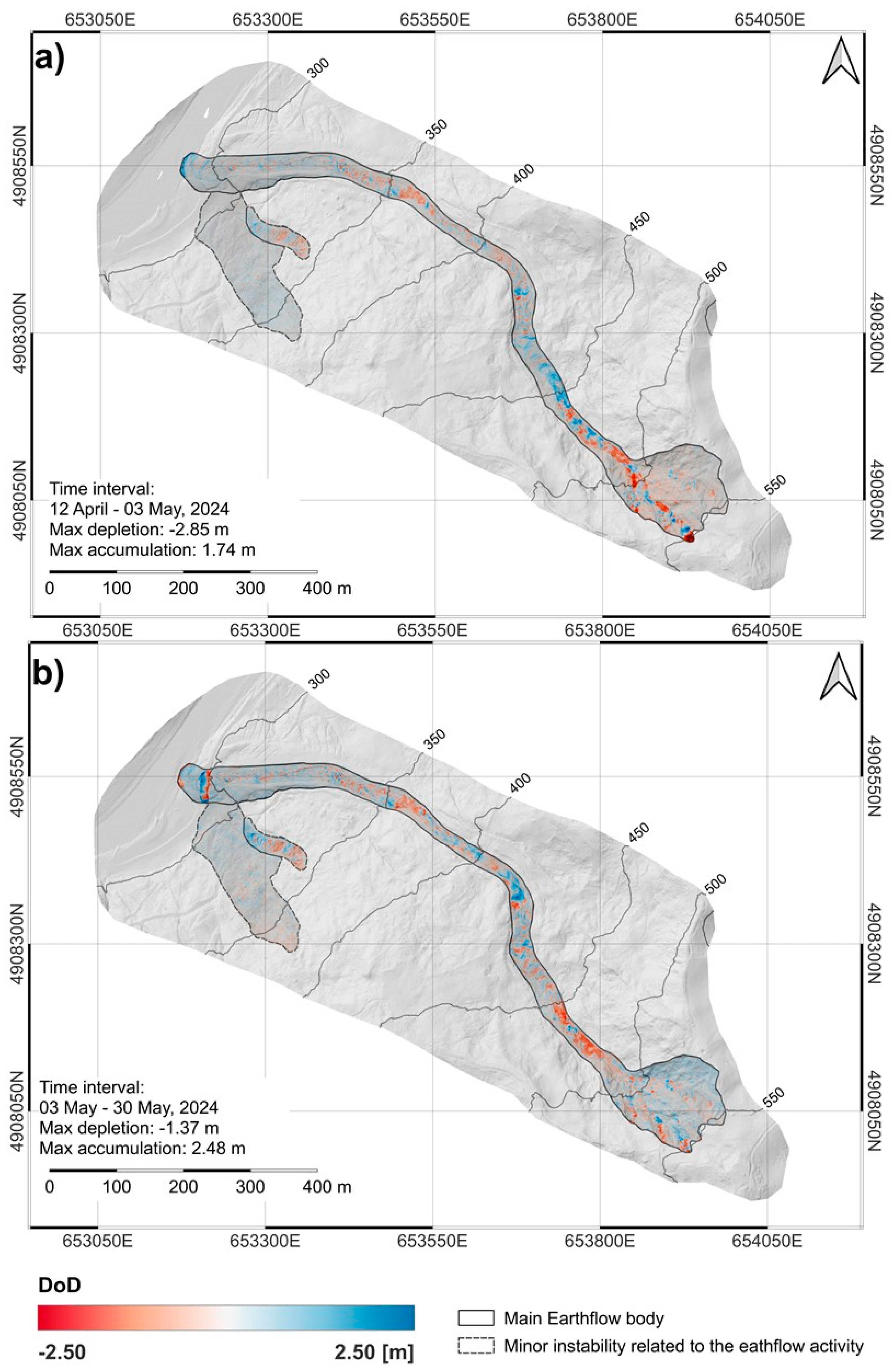
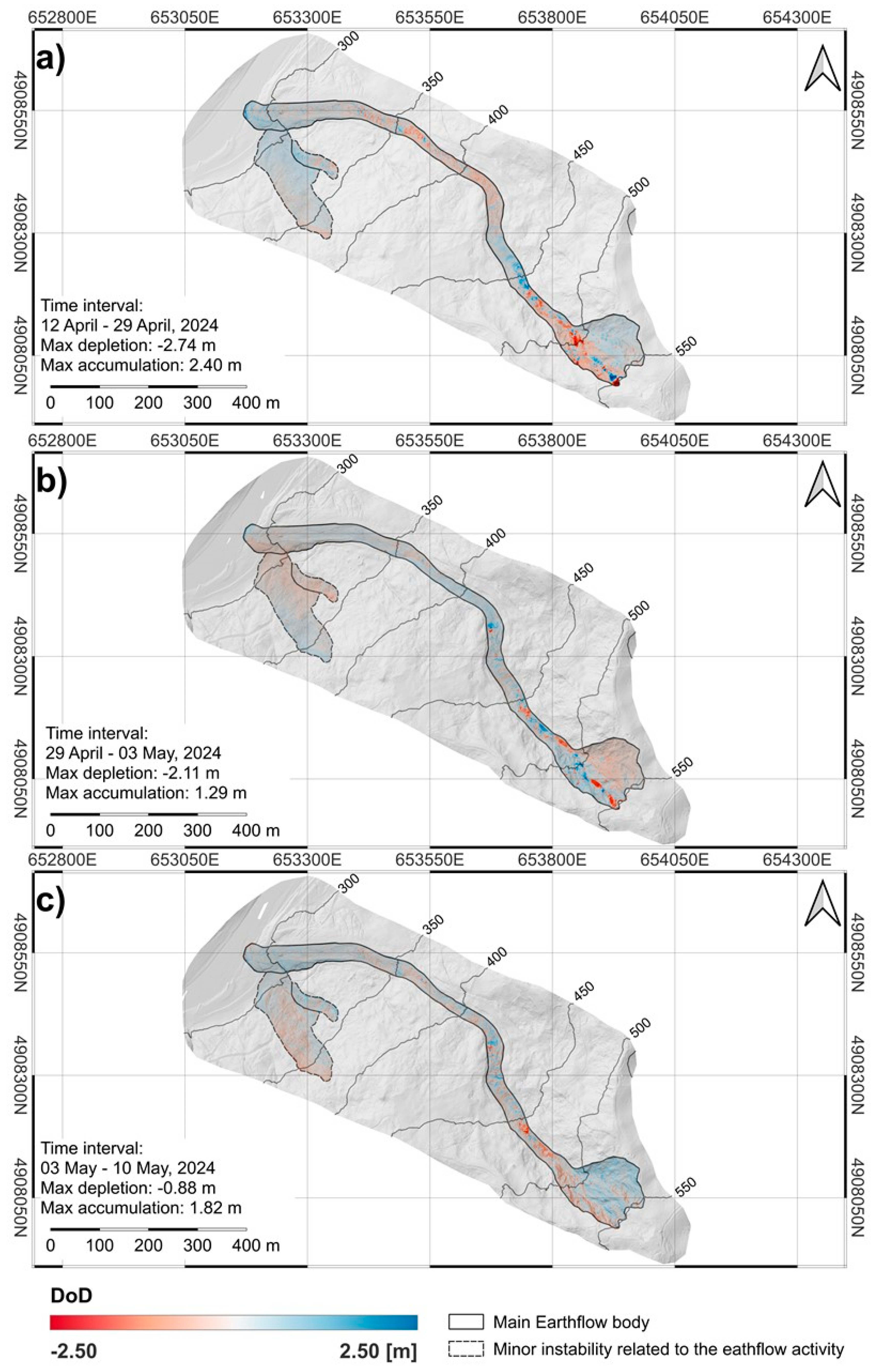
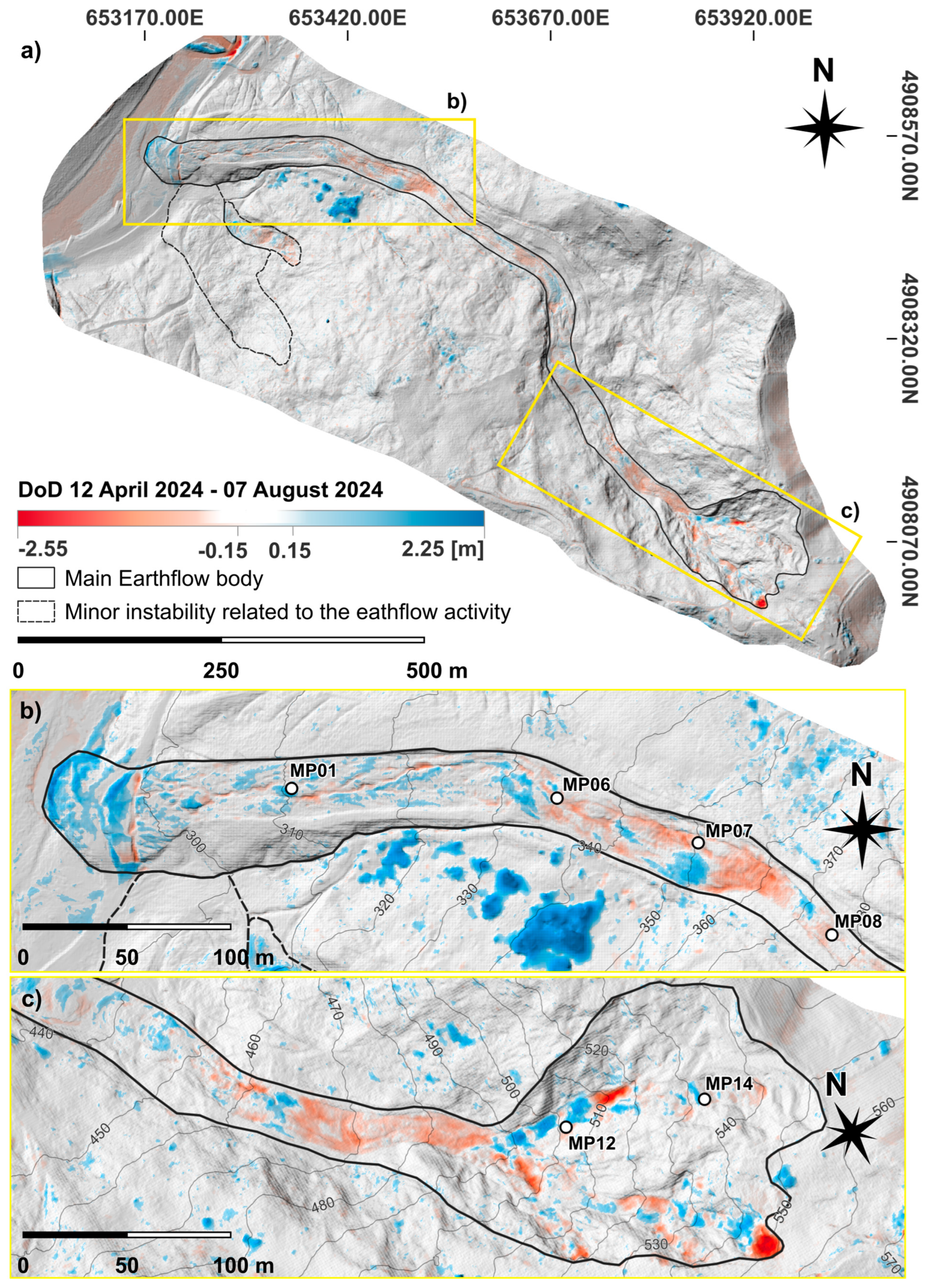
4.2. Results of DoD Analysis

The results of the DoDs refer to different temporal intervals (i.e.,: Full period, Alternating, Consecutive; see Figure 11 in the methods section for adopted temporal intervals). This allowed us to examine the spatial distribution of topographic changes and their evolution over the entire monitoring period as well as during it.

The results of Full period DoD (i.e., from 12 April to 7 August 2024) are shown in Figure 17a. A conservative threshold of ±15 cm is applied to exclude minor elevation differences within the expected vertical accuracy of the DEMs, thus reducing the influence of noise and registration error. In the toe area (Figure 17b), a broad accumulation zone can be seen, indicating elevation gain during the monitoring period. In the source area (Figure 17c), two distinct depletion areas are visible, particularly in the southern part. Outside the main landslide body, additional features are also present: the Panaro riverbed shows a general depletion pattern, with a small accumulation zone just downstream of the toe. Localized patches of accumulation are also visible along the left side of the track zone, likely caused by vegetation growth reducing the LiDAR sensor’s ground penetration over time.

A compilation of all four alternating DoD and nine consecutive DoD maps is presented in Appendix A. Alternating DoDs revealed activity phases over larger portions of the landslide, especially between late April and mid-May in the source area, and again between late June and early July in the track zone. Also, consecutive DoDs show that the most intense depletion event, located in the source area’s southern sector, occurred between 12 and 29 April 2024 and continued downslope between 29 April and 3 May 2024.

The DoD analysis provides insight into surface processes that may be difficult to capture with point-based techniques like RTS and HPT. Several intense elevation changes—such as those observed near HPs 12 and 14—are not recorded by the displacement data at those points. This is likely due to the localized nature of the reactivations, which may occur just a few meters away from the monitored targets. Furthermore, these reactivations often take the form of shallow slides or local mudflows, which may significantly change the surface morphology. In such cases, HPs may become unrecognizable, and MPs—mounted on rigid supports—can tilt or move, affecting their reliability. Furthermore, surface obstacles or local resistances may reduce the movement of natural features tracked by HPT, creating small but significant differences over time.

The spatial coverage offered by DoD maps is especially valuable in this context. Unlike RTS and HPT, which provide data from a limited number of points, the DoD method covers the entire surface. This makes it possible to detect activity that would otherwise remain unnoticed. Although DoD products do not measure displacement directly—since they represent elevation change at fixed positions—they still offer important insights into movement patterns when analyzed as a time series.

5. Discussion

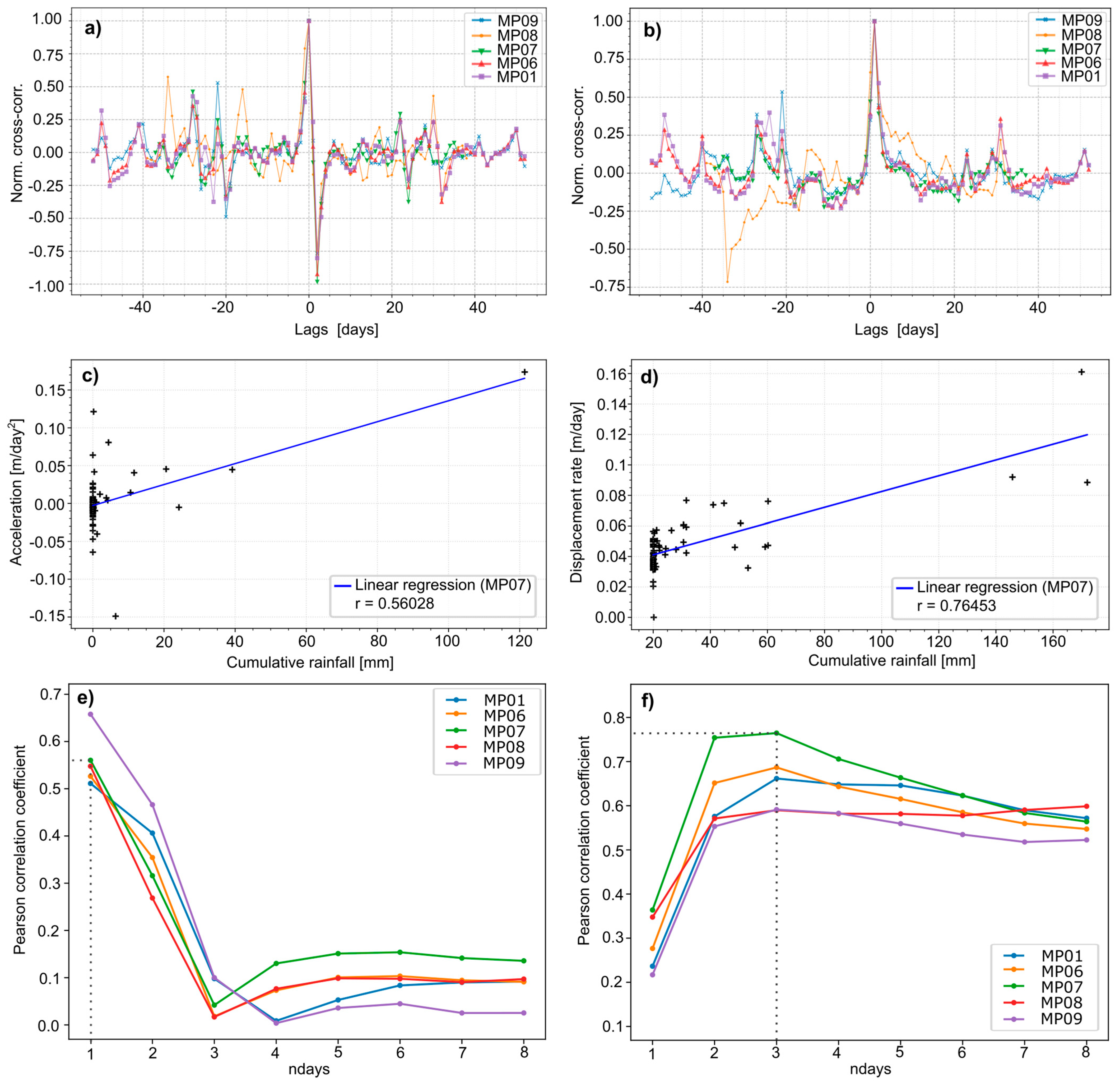
5.1. Insight on Earth-Flow Dynamics

The use of multitemporal HPT, DoD, and RTS data methods makes it possible to analyze the deformation behavior of the landslide with respect to rainfall and processes related to the downslope propagation of landslide deposits, which in earthflows typically determines progressive acceleration of movements that is commonly related to undrained loading mechanisms [45].

With respect to rainfall–movement relationships, high-frequency RTS displacement time series make it possible to carry out statistically based analysis. In this study, MPs with continuous data records were selected, specifically MP01, MP06, MP07, MP08, and MP09 (all located in the track zone). A normalized cross-correlation analysis was performed between rainfall and acceleration/velocity time series to investigate potential temporal relationships and response patterns. Results indicate that all the selected MPs tend to accelerate on the same day as rainfall peaks (Figure 18a), while they reach their maximum velocity 2–3 days later (Figure 18b), and tend to decelerate immediately after the rainfall event (see the negative correlation values in Figure 18a). The magnitude of acceleration and maximum velocity shows a linear correlation with the cumulated rainfall over different time windows. As an example, Figure 18c shows the linear correlation of MP07 acceleration values with respect to 1-day cumulated rainfall, while Figure 18d shows the linear correlation of MP07 velocity with respect to 3-day cumulated rainfall. The 1-day cumulated rainfall for acceleration and the 3-day cumulated rainfall for velocity are the time windows associated with the maximum Pearson correlation coefficient “r” for all the analyzed MPs (see Figure 18e,f). For instance, the “r” coefficient for MP acceleration and 1-day cumulated rainfall reaches values indicating a moderate to strong positive correlation, pointing to an almost immediate response of the landslide to rainfall events, confirming the previous normalized cross-correlation analysis. On the other hand, the “r” correlation coefficient for MP velocity and 3-day cumulated rainfall reaches values typical of a strong and positive correlation, pointing to a strong influence of rainfall cumulated over a few days in determining the significant displacement of the landslide masses. This behavior is consistent with the dynamics typically observed in the track zone of an earthflow, where the mobilized material is confined within well-defined boundaries and exhibits a high sensitivity to rainfall as the primary triggering factor.

With respect to the distribution of movements along the slope, the RTS and HPT offer detailed temporal tracking at distinct points, whereas the DoD reveals depletion and accumulation processes throughout the landslide. In the source area, DoD analysis reveals localized depletion zones, especially in the southern portion, indicating the occurrence of local slides and mudflow-like reactivations. At the same time, HPT/RTS data show displacement velocities that are generally below 1 m/month (i.e., 0.04–0.06 m/day recorded by MP12 and MP14 even during the acceleration event of 24 June 2024), alternated to sudden accelerations, that determining retrogression of the main scarp and the loss of MPs (so that the maximum velocity cannot be computed). In this sector, DoD maps also provide evidence of the role of retrogressive processes as drivers of the rapid downslope propagation of earthflows that, in turn, tend to destabilize track zone deposits. In the track zone, sequential DoDs evidence the alternation of depletion and accumulation phases observed. This evidences a wave-like propagation mechanism with pulses of movement, initiated by episodic releases from the source area, coupled with the remobilization of material downslope, with a visible pattern of erosion and deposition advancing over time. The HPT and RTS measurements reveal the variability of displacement rates, with the most active sector located in the upper and central track zones, with recorded displacements up to 5 m/month (with peaks of 0.8–1.1 m/day recorded by MP08 and MP09 during the acceleration event of 24 June 2024), which is characterized by steeper slopes and continuous flow-like behavior. In the lower track, velocities are reduced to 2.5–3.5 m/month, due to gentler terrain and material accumulation (with peaks of 0.4–0.6 m/day recorded by MP06 and MP07 during the acceleration event of 24 June 2024). In the toe zone, the DoD analysis highlights a progressive advancement of the landslide tip into the riverbed. This interaction appears to influence sediment dynamics in the track zone, as indicated by a confined accumulation zone immediately downstream of the toe. MPs and HPs velocities range from 1.5 to 2.5 m/month (with peaks of 0.20 m/day recorded by M01 during the acceleration event of 24 June 2024) and were higher in the central part of the fan-shaped deposit than at the flanks, part of which remained stable.

Overall, the interpretation emerging from the integrated dataset describes a complex deformation behaviour, with earth masses propagating from the source area down to the track and, finally, the toe zone responding as a whole to the rainfall trigger. As the earthflow moves downslope, the ongoing disaggregation and internal reworking lead to a more homogeneous flow, which evolves into a typical earthflow already in the upper part of the track zone. This transition reflects both the mechanical adaptation of the moving mass and the slope dynamics’ influence on slope geometry and confinement.

5.2. Operational and Technical Issues

Altogether, HPT and DoD provide a detailed and complementary dataset: while HPT offers precise displacement data on selected targets, DoD extends the spatial perspective, enabling a more complete understanding of the landslide’s dynamics.

The HPT has demonstrated high accuracy and operational flexibility. This method shows strong agreement with RTS in both displacement magnitude and velocity trends, confirming its reliability under real conditions. Its visual and non-contact nature makes it especially suitable for unsafe areas, and it can be applied freely across the UAV survey area without requiring physical installation. This operational simplicity gives HPT a practical advantage over RTS, which involves more demanding deployment and maintenance. It is also worthwhile to point out that, in our specific case, the impact of the RTS interruption on trend analysis and validation of HPT results was negligible, since the HPs did not show any significant acceleration of the landslide during the RTS interruption period. Furthermore, filling the RTS data gaps by using displacement interpolation from adjacent HPT points would cause more problems than benefits, as the time series of RTS used to validate HP tracking would, in that case, include data on the HPs themselves.

However, some limitations emerged during the study. The first is the need for visual continuity of homologous points between surveys, which may be compromised in rapidly changing or highly disturbed environments. HPT is therefore best suited to landslide types that preserve recognizable surface features between acquisitions, such as earthflows or rockslides, and is generally not applicable to processes like debris or mudflows, where material is fully reworked. Another limitation is the temporal resolution. While HPT can be repeated as often as needed, it cannot provide continuous data like RTS. As observed in the time series, this results in a smoothing of short-term accelerations and peaks occurring between acquisitions. Still, this effect can be reduced by adjusting the frequency of UAV surveys in more active conditions.

DoD analysis has proven to be particularly valuable for assessing the spatial complexity of landslide movement patterns. Its broad coverage enables the identification of reactivations and morphological changes that do not affect the monitored points, filling a key gap in point-based techniques. While DoDs do not represent true displacement—since they measure elevation change at fixed positions—they remain essential for interpreting slope behaviour in terms of depletion and accumulation.

5.3. Transferability of Methods and Broader Applications

The transferability of the adopted methods is very high for landslides characterized by significant displacement rates. UAV-based monitoring, particularly when supported by RTK positioning and LiDAR-derived topography, can be applied effectively to a wide range of landslides involving surface-preserving mass movements. The method is well-suited to processes ranging from extremely slow to rapid, as long as the surface morphology remains identifiable between surveys. Both the size and velocity of the landslide can be managed through the appropriate adjustment of survey frequency. Faster movements require denser temporal sampling, while spatial coverage can be optimized by selecting strategic sectors, depending on logistical constraints. Broader coverage increases the completeness and reliability of the overall interpretation.

The results of this study highlight the potential for using UAV monitoring in combination with other remote sensing or ground-based methods, as well as in a stand-alone system. The integration of UAV–LiDAR data with complementary satellite-based remote sensing techniques, such as radar interferometry or multispectral imagery analysis, can in principle deliver several benefits, such as improved kinematic interpretation, subdivision of landslide components into distinct kinematic zones, higher temporal seeding (e.g., filling gaps between UAV campaigns), and retrieval of multispectral indices (e.g., NDVI) to infer hydrological or vegetation-related instability precursors [46,47,48,49,50]. However, using these techniques on active earthflows moving at rates of several meters per week, such as the Baldiola case study, also has a significant number of limitations. For instance, multitemporal SAR interferometry returns too limited a number of scatterers inside the landslide area, and it is bound to largely underestimate displacement rates (as it is well known, it is suitable for phenomena moving cm/yr, and not m/day). For instance, the EGMS dataset 2019–2023 in our landslide area (https://egms.land.copernicus.eu/, accessed on 27 July 2025, see WGS84 44.3114N; 10.9276E) includes only a dozen scatterer points in the ascending and descending calibrated datasets combined, whose average velocities are very low and thus unrepresentative of the displacements in the landslide. No significant improvement is expected to arise from the application of site-specific distributed scatterer analysis or interferogram stacking techniques, since movement rates up to several meters in between two subsequent Sentinel-1 acquisitions are bound to determine a complete decorrelation of signals in a large part of the landslide. Also, the adoption of multispectral datasets to compute NDVI-changes is not expected to bring any significant added value to quantifying movement rates, as a large part of the source, track, and toe zones of the Baldiola earthflow have been substantially vegetation-free throughout the monitoring period, and the limited changes in vegetation cover observed due to retrogression of the crown could hardly be appreciated, for instance, with the 10 m pixel size of Sentinel-2 data.

For these reasons, data obtained using drone-based techniques (in this case, HPT and DoD analysis) coupled with RTS monitoring provide significant added value to monitoring of this kind of active earthflow phenomenon. This is because the displacement rates assessment proved sufficiently accurate and comprehensive to support both quantitative displacement analysis and qualitative interpretation of slope processes. In this context, the relevance of visual tracking approaches such as homologous point tracking (HPT) becomes particularly evident. While it may appear to be more manual and time-consuming than automated image correlation techniques, HPT offers a simple and effective solution that can significantly enhance the autonomy of UAV-based monitoring. Techniques such as digital image correlation or feature-based matching often require ground validation through RTS, GNSS, or similar systems. In contrast, HPT can serve as a direct, internally validated tracking method using only the UAV dataset. This opens up the possibility of achieving reliable displacement measurements without additional instrumentation, reinforcing the role of UAV photogrammetry as a comprehensive monitoring tool.

6. Conclusions

This study explores and demonstrates the effectiveness of UAV-based monitoring in assessing the kinematics of an active earthflow through the combined use of HPT and DoD methods. HPT, validated with RTS data, produces precise and coherent displacement trends across multiple sectors of the landslide. At the same time, DoD analysis provides essential information on the spatial distribution and timing of surface changes, especially in areas not covered with point-based measurements. Together, the two methods prove highly complementary, offering both point-based accuracy and spatially distributed interpretability.

The results obtained with UAV data support a detailed interpretation of the landslide’s internal dynamics, including local differences in movement patterns, retrogressive activity in the source area, and a pulsed propagation along the track zone. The consistency between HPT and RTS results, combined with the insights provided by DoD analysis, highlights the potential of UAV monitoring not only as a support tool but as a stand-alone system for landslide monitoring and assessment.

Beyond the technical performance, results prove the reliability of UAV-derived displacement data in real monitoring conditions. HPT is a practical alternative to external ground validation, as it enables internal consistency checks within the photogrammetric dataset. This approach could contribute to reducing the dependence on ground-based instruments for validating image-based tracking techniques such as digital image correlation and represents a viable path toward more autonomous UAV-based monitoring.

Future developments include the automation of displacement tracking through DIC algorithms validated via HPT, as well as a more systematic integration of rainfall data to better understand the triggering conditions and temporal evolution of the process. The approach presented here may also be extended to other types of slow-to-rapid landslides where surface morphology remains trackable over time.

In addition to its applicability and accuracy, UAV-based monitoring also offers a practical advantage in terms of operational flexibility. Once the quality of the photogrammetric data is established, the method can be applied even under suboptimal conditions or with limited field access. Its practical setup and the adaptability to different survey frequencies make it suitable not only for scientific investigation but also for high-frequency monitoring during critical phases of slope activity or in early emergency response.

The high temporal resolution adopted in this study demonstrates that UAV data acquisition can be tailored to the required pace of observation, supporting timely assessments in moderate to rapid landslide scenarios.

References

1. Chae, B.G.; Park, H.J.; Catani, F.; Simoni, A.; Berti, M. Landslide Prediction, Monitoring and Early Warning: A Concise Review of State-of-the-Art. Geosci. J. 2017, 21, 1033–1070. [Google Scholar] [CrossRef]
2. Catelan, F.T.; Bossi, G.; Schenato, L.; Tondo, M.; Critelli, V.; Mulas, M.; Ciccarese, G.; Corsini, A.; Tonidandel, D.; Mair, V.; et al. Long-Term Monitoring of Active Large-Scale Landslides for Non-Structural Risk Mitigation—Integrated Sensors and Web-Based Platform. J. Mt. Sci. 2025, 22, 1–15. [Google Scholar] [CrossRef]
3. Mantovani, M.; Bossi, G.; Dykes, A.P.; Pasuto, A.; Soldati, M.; Devoto, S. Coupling Long-Term GNSS Monitoring and Numerical Modelling of Lateral Spreading for Hazard Assessment Purposes. Eng. Geol. 2022, 296, 106466. [Google Scholar] [CrossRef]
4. Casagli, N.; Intrieri, E.; Tofani, V.; Gigli, G.; Raspini, F. Landslide Detection, Monitoring and Prediction with Remote-Sensing Techniques. Nat. Rev. Earth Environ. 2023, 4, 51–64. [Google Scholar] [CrossRef]
5. Corsini, A.; Bonacini, F.; Mulas, M.; Petitta, M.; Ronchetti, F.; Truffelli, G. Long-Term Continuous Monitoring of a Deep-Seated Compound Rock Slide in the Northern Apennines (Italy). In Engineering Geology for Society and Territory—Volume 2: Landslide Processes; Springer International Publishing: Cham, Switzerland, 2015; pp. 1337–1340. [Google Scholar] [CrossRef]
6. Critelli, V.; Ronchetti, F.; Berti, M.; Bernardi, A.R.; Caputo, G.; Ciccarese, G.; Mulas, M.; Bernardi, M.; Corsini, A. Slope Response to Effective Rainfall of a Large, Complex Rock-Slide in Flysch Material. Ital. J. Eng. Geol. Environ. 2024, 77–84. [Google Scholar] [CrossRef]
7. Glueer, F.; Loew, S.; Seifert, R.; Aaron, J.; Grämiger, L.; Conzett, S.; Limpach, P.; Wieser, A.; Manconi, A. Robotic Total Station Monitoring in High Alpine Paraglacial Environments: Challenges and Solutions from the Great Aletsch Region (Valais, Switzerland). Geosciences 2021, 11, 471. [Google Scholar] [CrossRef]
8. Corsini, A.; Baiguera, G.; Capuano, F.; Ciccarese, G.; Diena, M.; Mulas, M.; Ronchetti, F.; Rossi, G.; Truffelli, G. Micropiles Tripods Shields (MTS) as Unconventional Breakers for the Control of Moderately Rapid Earthflows (Sassi Neri Landslide, Northern Apennines). Ital. J. Eng. Geol. Environ. 2021, 35–45. [Google Scholar] [CrossRef]
9. Lucieer, A.; de Jong, S.M.; Turner, D. Mapping Landslide Displacements Using Structure from Motion (SfM) and Image Correlation of Multi-Temporal UAV Photography. Prog. Phys. Geogr. 2014, 38, 97–116. [Google Scholar] [CrossRef]
10. Azmoon, B.; Biniyaz, A.; Liu, Z. Use of High-Resolution Multi-Temporal DEM Data for Landslide Detection. Geosciences 2022, 12, 378. [Google Scholar] [CrossRef]
11. Godone, D.; Allasia, P.; Borrelli, L.; Gullà, G. UAV and Structure from Motion Approach to Monitor the Maierato Landslide Evolution. Remote Sens. 2020, 12, 1039. [Google Scholar] [CrossRef]
12. Giordan, D.; Hayakawa, Y.S.; Nex, F.; Tarolli, P. Preface: The Use of Remotely Piloted Aircraft Systems (RPAS) in Monitoring Applications and Management of Natural Hazards. Nat. Hazards Earth Syst. Sci. 2018, 18, 3085–3087. [Google Scholar] [CrossRef]
13. Huang, H.; Long, J.; Yi, W.; Yi, Q.; Zhang, G.; Lei, B. A Method for Using Unmanned Aerial Vehicles for Emergency Investigation of Single Geo-Hazards and Sample Applications of This Method. Nat. Hazards Earth Syst. Sci. 2017, 17, 1961–1979. [Google Scholar] [CrossRef]
14. Westoby, M.J.; Brasington, J.; Glasser, N.F.; Hambrey, M.J.; Reynolds, J.M. “Structure-from-Motion” Photogrammetry: A Low-Cost, Effective Tool for Geoscience Applications. Geomorphology 2012, 179, 300–314. [Google Scholar] [CrossRef]
15. Tondo, M.; Mulas, M.; Ciccarese, G.; Marcato, G.; Bossi, G.; Tonidandel, D.; Mair, V.; Corsini, A. Detecting Recent Dynamics in Large-Scale Landslides via the Digital Image Correlation of Airborne Optic and LiDAR Datasets: Test Sites in South Tyrol (Italy). Remote Sens. 2023, 15, 2971. [Google Scholar] [CrossRef]
16. Turner, D.; Lucieer, A.; de Jong, S.M. Time Series Analysis of Landslide Dynamics Using an Unmanned Aerial Vehicle (UAV). Remote Sens. 2015, 7, 1736–1757. [Google Scholar] [CrossRef]
17. Brook, M.S.; Merkle, J. Monitoring Active Landslides in the Auckland Region Utilising UAV/Structure-from-Motion Photogrammetry. Jpn Geotech. Soc. Spec. Publ. 2019, 6, 1–6. [Google Scholar] [CrossRef]
18. Stringer, J.; Brook, M.S.; Justice, R. Post-Earthquake Monitoring of Landslides along the Southern Kaikōura Transport Corridor, New Zealand. Landslides 2021, 18, 409–423. [Google Scholar] [CrossRef]
19. Izumida, A.; Uchiyama, S.; Sugai, T. Application of UAV-SfM Photogrammetry and Aerial Lidar to a Disastrous Flood: Repeated Topographic Measurement of a Newly Formed Crevasse Splay of the Kinu River, Central Japan. Nat. Hazards Earth Syst. Sci. 2017, 17, 1505–1519. [Google Scholar] [CrossRef]
20. Saroglou, C.; Asteriou, P.; Zekkos, D.; Tsiambaos, G.; Clark, M.; Manousakis, J. UAV-Based Mapping, Back Analysis and Trajectory Modeling of a Coseismic Rockfall in Lefkada Island, Greece. Nat. Hazards Earth Syst. Sci. 2018, 18, 321–333. [Google Scholar] [CrossRef]
21. Dai, K.; Li, Z.; Xu, Q.; Tomas, R.; Li, T.; Jiang, L.; Zhang, J.; Yin, T.; Wang, H. Identification and Evaluation of the High Mountain Upper Slope Potential Landslide Based on Multi-Source Remote Sensing: The Aniangzhai Landslide Case Study. Landslides 2023, 20, 1405–1417. [Google Scholar] [CrossRef]
22. Minervino Amodio, A.; Corrado, G.; Gallo, I.G.; Gioia, D.; Schiattarella, M.; Vitale, V.; Robustelli, G. Three-Dimensional Rockslide Analysis Using Unmanned Aerial Vehicle and LiDAR: The Castrocucco Case Study, Southern Italy. Remote Sens. 2024, 16, 2235. [Google Scholar] [CrossRef]
23. Ciccarese, G.; Tondo, M.; Mulas, M.; Bertolini, G.; Corsini, A. Rapid Assessment of Landslide Dynamics by UAV-RTK Repeated Surveys Using Ground Targets: The Ca’ Lita Landslide (Northern Apennines, Italy). Remote Sens. 2024, 16, 1032. [Google Scholar] [CrossRef]
24. Martínez-Carricondo, P.; Agüera-Vega, F.; Carvajal-Ramírez, F. Accuracy Assessment of RTK/PPK UAV-Photogrammetry Projects Using Differential Corrections from Multiple GNSS Fixed Base Stations. Geocarto Int. 2023, 38, 2197507. [Google Scholar] [CrossRef]
25. Taddia, Y.; Stecchi, F.; Pellegrinelli, A. Using Dji Phantom 4 Rtk Drone for Topographic Mapping of Coastal Areas. Int. Arch. Photogramm. Remote Sens. Spat. Inf. Sci.—ISPRS Arch. 2019, 42, 625–630. [Google Scholar] [CrossRef]
26. Kalacska, M.; Lucanus, O.; Arroyo-Mora, J.P.; Laliberté, É.; Elmer, K.; Leblanc, G.; Groves, A. Accuracy of 3D Landscape Reconstruction without Ground Control Points Using Different Platforms. Drones 2020, 4, 13. [Google Scholar] [CrossRef]
27. Stott, E.; Williams, R.D.; Hoey, T.B. Ground Control Point Distribution for Accurate Kilometre-Scale Topographic Mapping Using an RTK-GNSS Unmanned Aerial Vehicle and SfM Photogrammetry. Drones 2020, 4, 55. [Google Scholar] [CrossRef]
28. Dematteis, N.; Wrzesniak, A.; Allasia, P.; Bertolo, D.; Giordan, D. Integration of Robotic Total Station and Digital Image Correlation to Assess the Three-Dimensional Surface Kinematics of a Landslide. Eng. Geol. 2022, 303, 106655. [Google Scholar] [CrossRef]
29. Bickel, V.T.; Manconi, A.; Amann, F. Quantitative Assessment of Digital Image Correlation Methods to Detect and Monitor Surface Displacements of Large Slope Instabilities. Remote Sens. 2018, 10, 865. [Google Scholar] [CrossRef]
30. Mulas, M.; Ciccarese, G.; Truffelli, G.; Corsini, A. Integration of Digital Image Correlation of Sentinel-2 Data and Continuous Gnss for Long-Term Slope Movements Monitoring in Moderately Rapid Landslides. Remote Sens. 2020, 12, 2605. [Google Scholar] [CrossRef]
31. Gioia, D.; Corrado, G.; Minervino Amodio, A.; Schiattarella, M. Multi-Temporal Morphological Analysis Coupled to Seismic Survey of a Mass Movement from Southern Italy: A Combined Tool to Unravel the History of Complex Slow-Moving Landslides. Nat. Hazards 2024, 120, 13407–13432. [Google Scholar] [CrossRef]
32. Parente, C.; Pepe, M. Uncertainty in Landslides Volume Estimation Using DEMs Generated by Airborne Laser Scanner and Photogrammetry Data. Int. Arch. Photogramm. Remote Sens. Spat. Inf. Sci.—ISPRS Arch. 2018, 42, 397–404. [Google Scholar] [CrossRef]
33. Bossi, G.; Cavalli, M.; Crema, S.; Frigerio, S.; Quan Luna, B.; Mantovani, M.; Marcato, G.; Schenato, L.; Pasuto, A. Multi-Temporal LiDAR-DTMs as a Tool for Modelling a Complex Landslide: A Case Study in the Rotolon Catchment (Eastern Italian Alps). Nat. Hazards Earth Syst. Sci. 2015, 15, 715–722. [Google Scholar] [CrossRef]
34. Lane, S.N.; Westaway, R.M.; Hicks, D.M. Estimation of Erosion and Deposition Volumes in a Large, Gravel-Bed, Braided River Using Synoptic Remote Sensing. Earth Surf. Process Landf. 2003, 28, 249–271. [Google Scholar] [CrossRef]
35. Corsini, A.; Borgatti, L.; Cervi, F.; Dahne, A.; Ronchetti, F.; Sterzai, P. Estimating Mass-Wasting Processes in Active Earth Slides—Earth Flows with Time-Series of High-Resolution DEMs from Photogrammetry and Airborne LiDAR. Nat. Hazards Earth Syst. Sci. 2009, 9, 433–439. [Google Scholar] [CrossRef]
36. Bettelli, G.; Panini, F.; Pizziolo, M. Carta Geologica d’Italia Alla Scala 1:50.000—Foglio 236 Pavullo Nel Frignano. 2002. Available online: https://www.openaccessrepository.it/records/0eeby-dww93 (accessed on 27 July 2025).
37. Regione Emilia-Romagna. Servizi OGC—Elenco Capabilities Dei Servizi WMS. Geoportale Regione Emilia-Romagna. Available online: https://geoportale.regione.emilia-romagna.it/servizi/servizi-ogc/elenco-capabilities-dei-servizi-wms (accessed on 9 December 2024).
38. Bettelli, G.; Panini, F. Introduction to the Geology of the South-Eastern Sector of the Emilia Apennines, Guide to the Northern Apennine Traverse. In Proceedings of the 76th Summer Meeting-Congress of the Italian Geological Society (SGI), Florence, Italy, 16–20 September 1992; pp. 207–240. [Google Scholar]
39. Cruden, D.M.; Varnes, D.J. Landslide Types and Processes. In Landslides: Investigation and Mitigation; National Academy Press: Washington, DC, USA, 1996; Volume Special Report 247, pp. 36–75. ISBN 030906208X. [Google Scholar]
40. Regione Emilia-Romagna. L’archivio Storico Dei Movimenti Franosi. Regione Emilia-Romagna Geoportale. Available online: https://ambiente.regione.emilia-romagna.it/it/geologia/geologia/dissesto-idrogeologico/larchivio-storico-dei-movimenti-franosi (accessed on 4 November 2024).
41. Google Earth Pro, Version 7.3.6; Google LLC: Mountain View, CA, USA, 2025.
42. Mesas-Carrascosa, F.J.; García, M.D.N.; De Larriva, J.E.M.; García-Ferrer, A. An Analysis of the Influence of Flight Parameters in the Generation of Unmanned Aerial Vehicle (UAV) Orthomosaics to Survey Archaeological Areas. Sensors 2016, 16, 1838. [Google Scholar] [CrossRef]
43. DJI. DJI Terra, Version 4.3.0; DJI Technology Co., Ltd.: Shenzhen, China, 2025.
44. QGIS.org. QGIS Geographic Information System, Version 3.36; Open Source Geospatial Foundation Project. 2025. Available online: https://www.qgis.org (accessed on 21 January 2025).
45. Hutchinson, J.N.; Bhandari, R.K. Undrained Loading, A Fundamental Mechanism of Mudflows and Other Mass Movements. Géotechnique 1971, 21, 353–358. [Google Scholar] [CrossRef]
46. Torre, D.; Zocchi, M.; Iacobucci, G.; Menichetti, M.; Toselli, R.; Troiani, F.; Piacentini, D. Morphoevolutive Drivers on a Rapidly-Evolving Soft Rocky Cliff and Connected Shore Platform System. Earth Surf. Process Landf. 2025, 50, e70117. [Google Scholar] [CrossRef]
47. Zocchi, M.; Delchiaro, M.; Troiani, F.; Scarascia Mugnozza, G.; Mazzanti, P. PS-InSAR Post-Processing for Assessing the Spatio-Temporal Differential Kinematics of Complex Landslide Systems: A Case Study of DeBeque Canyon Landslide (Colorado, USA). Earth Surf. Process Landf. 2024, 49, 4862–4880. [Google Scholar] [CrossRef]
48. Okyay, U.; Telling, J.; Glennie, C.L.; Dietrich, W.E. Airborne Lidar Change Detection: An Overview of Earth Sciences Applications. Earth Sci. Rev. 2019, 198, 102929. [Google Scholar] [CrossRef]
49. Meng, Y.; Lan, H.; Li, L.; Wu, Y.; Li, Q. Characteristics of Surface Deformation Detected by X-Band SAR Interferometry over Sichuan-Tibet Grid Connection Project Area, China. Remote Sens. 2015, 7, 12265–12281. [Google Scholar] [CrossRef]
50. Mora, O.; Lenzano, M.; Toth, C.; Grejner-Brzezinska, D.; Fayne, J. Landslide Change Detection Based on Multi-Temporal Airborne LiDAR-Derived DEMs. Geosciences 2018, 8, 23. [Google Scholar] [CrossRef]
Figure 1. Geological and geographical setting of the Baldiola landslide. On the left, a geological map of the study area from the Emilia-Romagna region official WMS geological dataset. Reference system: WGS84 UTM Zone 32N, EPSG:32632).
Remotesensing 17 02657 g001
Figure 2. Overview of the main evolution steps of the Baldiola landslide over time based on satellite image reconstruction (Google Earth and available Emilia Romagna WMS). (a) Toe area widening; (b) Source area retrogression. Base map: UAV survey, 12 April 2024. Reference system: WGS84 UTM Zone 32N (EPSG:32632).
Remotesensing 17 02657 g002
Figure 3. Conceptual workflow illustrating the three main phases of the study: survey methods, data acquisition, and data processing (red, orange); slope movements assessment (green), and earthflow dynamics assessment (blue).
Remotesensing 17 02657 g003
Figure 4. Conceptual illustration of the difference between HPT vertical displacement tracking and elevation change detection via DoD. The vertical component in HPT is calculated by retrieving the elevation at the updated position of a moving point (P) in each DEM. Conversely, DoD evaluates elevation changes at fixed spatial coordinates by subtracting DEMs acquired at different times.
Remotesensing 17 02657 g004
Figure 5. Map of the Baldiola landslide showing the location of the RTS and the four RPs (a), and the initial positions of the 18 MPs across the landslide body (b). Base map: UAV survey, 12 April 2024. Reference system: WGS84 UTM Zone 32N (EPSG:32632).
Remotesensing 17 02657 g005
Figure 6. Verification of the stability of the RTS pillar and benchmark where the DJI D-RTK 2 mobile station is periodically placed. (a) Hourly relative RTS coordinates calculated in free-station mode; (b) Relative RTS coordinates time-series: easting (1), northing (2); (c) The red box contains the position of man-made structures (zoomed in figure (d,e)) used as evidence of the precision of survey georeferencing; (d) Hillshade of man-made structures from LiDAR data on 12 April 2024; (e) Hillshade of man-made structures from LiDAR data on 7 August 2024. Reference system: WGS84 UTM Zone 32N (EPSG:32632).
Remotesensing 17 02657 g006
Figure 7. Comparison of DEMs (visualized as hillshades) and DoDs at different resolutions. (a) 5 cm/px DEM (3 May 2024); (b) 15 cm/px DEM (3 May 2024); (c) 25 cm/px DEM (3 May 2024); (d) DoD at 5 cm/px (29 April 2024 to 3 May 2024); (e) DoD at 15 cm/px (29 April 2024 to v May 2024); (f) DoD at 5 cm/px (29 April 2024 to 3 May 2024). Base map for (df): hillshade of 3 May 2024. Reference system: WGS84 UTM Zone 32N (EPSG:32632).
Remotesensing 17 02657 g007
Figure 8. Landslide map showing the initial positions of the analyzed HPs, including those associated with an MP (subset 1, red triangles) and those located in areas not visible from the RTS (subset 2). For subset 1, MP positions are also shown as white dots. Base map, UAV survey, 12 April 2024. Reference system: WGS84 UTM Zone 32N (EPSG:32632).
Remotesensing 17 02657 g008
Figure 9. Examples of HPs identified on the orthophotos. Red dashed boxes indicate the tracked object; white dots show the selected fixed point as a reference for tracking. (a) HP08, (b) HP05, (c) HP19, (d) HP03, (e) HP03h, (f) HP04h.
Remotesensing 17 02657 g009
Figure 10. Example of HPT applied to HP01 over the time interval from 12 April 2024 to 7 August 2024. (a) HP01 location. (b) Horizontal displacement derived from multi-temporal orthomosaics. (c) Vertical displacement derived from DEMs. Yellow arrows indicate the displacement direction across dates. Base map: UAV survey, 12 April 2024. Reference system: WGS84 UTM Zone 32N (EPSG:32632).
Remotesensing 17 02657 g010
Figure 11. Temporal sampling schemes used for DoD analysis over the April–August 2024 monitoring period. Each row represents a different temporal strategy, with bars indicating the time intervals used to generate DoD maps.
Remotesensing 17 02657 g011
Figure 12. MPs (a) and HPs (b) classified based on cumulated displacement over the monitoring period. The size of the triangles (MPs and HPs from subset 1) and circles (HPs from subset 2) varies proportionally with the magnitude of total displacement. Base map: UAV LiDAR survey, 7 August 2024. Reference system: WGS84 UTM Zone 32N (EPSG:32632).
Remotesensing 17 02657 g012
Figure 13. Time series of cumulative horizontal displacements recorded by RTS and HPT for selected HPs and their associated MPs. Solid lines represent RTS data, while colored markers indicate HPT measurements. (a) MPs and corresponding HPs (subset 1); (b) stand-alone HPs (subset 2). UAV survey dates are marked along the timeline; (c) daily and cumulated rainfall.
Remotesensing 17 02657 g013
Figure 14. Time series of cumulative vertical displacements recorded by RTS and HPT for selected HPs and their associated MPs. Solid lines represent RTS data, while colored markers indicate HPT measurements. (a) MPs and corresponding HPs (subset 1); (b) stand-alone HPs (subset 2). UAV survey dates are marked along the timeline; (c) daily and cumulated rainfall.
Remotesensing 17 02657 g014
Figure 15. Comparison between horizontal displacement data from RTS and HPT. (a) Scatterplot showing direct comparison of cumulative displacements. The red dashed line represents the trend (regression), while the grey line indicates the 1:1 reference. (b) Relative error of HPT measurements with respect to RTS values. The red curve shows the best-fit power law; yellow and orange dashed lines represent 25% and 50% error thresholds, corresponding to 0.99 m and 0.38 m, respectively.
Remotesensing 17 02657 g015
Figure 16. Comparison of vertical displacement data from RTS and HPT. (a) Scatterplot showing direct comparison of cumulative vertical displacements. The red dashed line indicates the regression trend, while the grey line represents the 1:1 reference. (b) Relative error of HPT measurements with respect to RTS values. The red curve shows the best-fit power law; yellow and orange dashed lines represent 25% and 50% error thresholds. Due to the poor fit, these percentages cannot be used to estimate associated vertical displacement values.
Remotesensing 17 02657 g016
Figure 17. DoD cumulative map between 12 April and 7 August 2024, highlighting areas of accumulation (blue) and depletion (red) along the landslide. (a) Overview of the main earthflow body and surrounding minor instabilities; (b,c) zoomed views of the toe and source areas, respectively. Active MPs are represented by white dots.
Remotesensing 17 02657 g017
Figure 18. Statistical analysis assessing selected MPs’ responses to rainfalls. (a) Cross-correlation between acceleration and daily rainfall time-series; (b) Cross-correlation between velocity and daily rainfall time-series; (c) Acceleration of MP07 vs. 1-day cumulated rainfall; (d) Velocity of MP07 vs. 3-day cumulated rainfall; (e) Pearson correlation coefficient for acceleration vs. 1- to 8-day cumulated rainfall; (f) Pearson correlation coefficient for velocity vs. 1- to 8-day cumulated rainfall.
Remotesensing 17 02657 g018