Small but Mighty: A Lightweight Feature Enhancement Strategy for LiDAR Odometry in Challenging Environments

Abstract

LiDAR-based Simultaneous Localization and Mapping (SLAM) serves as a fundamental technology for autonomous navigation. However, in complex environments, LiDAR odometry often experience degraded localization accuracy and robustness. This paper proposes a computationally efficient enhancement strategy for LiDAR odometry, which improves system performance by reinforcing high-quality features throughout the optimization process. For non-ground features, the method employs statistical geometric analysis to identify stable points and incorporates a contribution-weighted optimization scheme to strengthen their impact in point-to-plane and point-to-line constraints. In parallel, for ground features, locally stable planar surfaces are fitted to replace discrete point correspondences, enabling more consistent point-to-plane constraint formulation during ground registration. Experimental results on the KITTI and M2DGR datasets demonstrated that the proposed method significantly improves localization accuracy and system robustness, while preserving real-time performance with minimal computational overhead. The performance gains were particularly notable in scenarios dominated by unstructured environments.

1. Introduction

Simultaneous Localization and Mapping (SLAM) is a fundamental capability in autonomous robotics, enabling a robot to construct a map of an unknown environment while simultaneously estimating its own pose. Depending on the sensing modality, SLAM is commonly categorized into visual SLAM [1,2,3] and LiDAR-based SLAM [4,5,6]. Compared with cameras, LiDAR sensors provide higher range accuracy and are more robust to illumination changes, making them suitable for applications, such as autonomous driving [7], robotic navigation [8], and high-precision map generation [9].

Among LiDAR SLAM techniques, feature-based odometry remains a prominent research focus due to its favorable efficiency and accuracy. These methods primarily rely on extracting geometric features from point clouds using feature extractors and constructing residual constraints for pose estimation. LOAM [10], a representative method in this category, extracts edge and planar features and estimates the sensor’s pose by minimizing point-to-line and point-to-plane residuals. However, the performance of feature-based odometry is largely dependent on the stability and accuracy of the feature extraction process, which poses a significant limitation in complex environments. Complex environments typically refer to diverse scenarios, including both indoor and outdoor settings, with varied road conditions, irregular terrains, and complex spatial layouts, where the reliability of geometric features can be severely affected. In particular, certain subsets of these environments introduce strong challenges for LiDAR odometry due to the lack of distinct or stable structural cues.

To mitigate this issue, one line of research focuses on enhancing the reliability of feature constraints by refining the feature extraction process. For instance, several methods enhance feature discriminability and suppress erroneous correspondences by filtering small point clusters [11] and various types of outliers [12], applying principal component analysis [13] and local covariance matrix estimation [14], incorporating eigenvalue-based evaluation [14] and geometric consistency validation [15].

Another line of research aims to enrich the representational capacity of features by introducing higher-dimensional constraints into the optimization framework. For example, some approaches introduce CAD models [16], triangular meshes [17], semantic labels [18,19], geometric primitives, such as lines and cylinders [20], and intensity information [21] to enrich the feature space and provide additional sources of constraint for pose estimation.

Despite these advancements, such methods face several limitations. On one hand, their performance gains still depend on the reliability of the feature extractors and the quality of geometric features in the environment. On the other hand, during feature point matching, all features are usually treated equally without distinguishing their contributions to pose estimation. In challenging environments, including unstructured terrains [22], such as hills, scrublands, rural roads and forested areas, and geometrically uninformative spaces [23], such as corridors that lack clear planar and linear features, low-quality or unstable residuals may dominate the optimization process, often leading to local minima or significant degradation in odometry accuracy. To address these limitations, we propose FE-LOAM (Feature Enhancement LiDAR Odometry), a small but powerful LiDAR odometry framework built upon LeGO-LOAM, which incorporates a lightweight and effective feature enhancement strategy to significantly improve pose estimation robustness and accuracy by leveraging stable features. The core mechanism of FE-LOAM lies in a stability-aware enhancement strategy that selects stable feature points based on the statistical distribution of neighborhood curvature and adaptively adjusts their contribution during the optimization process. This enables the system to effectively amplify the role of limited high-confidence features in both structured and unstructured environments, thereby improving odometry accuracy and robustness under varying geometric conditions.

The main contributions of this work are summarized as follows:

• A stability-aware feature selection mechanism based on the statistical distribution of local smoothness is proposed to efficiently identify stable features from conventional geometric feature extractions.
• An adaptive weighting scheme is introduced to emphasize stable features during pose optimization, thereby suppressing the influence of low-quality residuals and enhancing estimation robustness.
• Extensive experiments on challenging datasets demonstrate consistent performance gains across diverse environments, validating the generality of the proposed strategy.

2. Related Work

The robustness and accuracy of LiDAR odometry are essential for achieving high-precision localization and mapping in autonomous robotic systems. The performance of 3D LiDAR odometry largely depends on the quality of feature correspondences established during sequential point cloud registration. Among LiDAR SLAM methodologies, feature-based approaches remain a primary research focus due to their computational efficiency and flexibility in integration.

The development of LiDAR odometry has advanced considerably, progressing from 2D to 3D systems, purely LiDAR-based approaches to multi-modal solutions, and from geometric methods to approaches incorporating deep learning techniques. While multi-modal odometry has seen rapid development in recent years, leveraging sensor redundancy and data fusion through techniques, such as tight coupling with inertial navigation systems (INS) [24,25], camera-LiDAR fusion [26,27], and GNSS integration [28,29] to overcome certain limitations, LiDAR odometry itself remains a fundamental component. The study and refinement of purely LiDAR odometry continues to be of significant research interest, with ongoing efforts dedicated to improving its reliability, precision, and adaptability in increasingly complex environments.

Additionally, recent research has explored the use of deep learning techniques for 3D LiDAR odometry estimation [30,31,32], in which neural networks are employed to replace traditional feature extractors for identifying distinctive points, followed by residual construction and pose estimation. Beyond interpretability concerns, deep learning approaches also demand substantial computational resources requiring dedicated GPU hardware and exhibit limited generalization to unseen environments. Consequently, despite their expressive capacity, geometry-based methods remain widely adopted in both academic research and industrial deployments.

Among geometry-based methods, feature-based methods [33] represent the most extensively studied and widely implemented framework, characterized by decades of algorithmic refinement and well-understood operational principles. Feature-based methods extract geometrically distinctive features from point clouds and perform frame-to-frame registration based on these correspondences, enabling efficient and accurate pose estimation. LOAM [10] is a representative algorithm in this category. It classifies edge and planar features using local smoothness scores, and estimates poses via point-to-line [34] and point-to-plane [35] ICP algorithms. F-LOAM [36], a variant of LOAM, introduces a non-iterative two-stage distortion compensation method that significantly improves both efficiency and robustness.

Despite their advantages, feature-based methods still exhibit limitations. Their performance heavily relies on the stability and accuracy of the feature extractor, making them susceptible to failure in structurally complex or feature-sparse environments caused by feature degradation or mismatches. To address these challenges, a variety of methods have been proposed.

One line of improvement focuses on refining the feature extraction process to increase the quality of features used in optimization. For instance, LeGO-LOAM [11] improves accuracy and computational efficiency by segmenting the ground and filtering small point clusters to eliminate invalid features. KFS-LIO [37] discards low-contributing matches through a quantitative evaluation of feature constraints, enhancing real-time performance. Liang et al. [14] extended the LiDAR odometry framework by introducing an eigenvalue-based feature analysis method, which identifies and emphasizes salient features during matching by evaluating their eigenvalue characteristics. Liu et al. [38] employ inter-frame clustering and tracking to filter outliers and reinforce ground constraints. To enhance feature quality, Guo et al. [39] apply principal component analysis (PCA) to evaluate curvature and extract high-quality edge and planar features. FEVO-LOAM [13] classifies points based on neighborhood covariance matrices and curvature, while also incorporating vertical and pitch residuals into the objective function in scenes with significant elevation changes. Finally, Light-LOAM [15] enhances registration robustness in feature-sparse environments by combining graph-based matching with geometric consistency checks.

Another research direction focuses on expanding the types and expressiveness of features to enhance SLAM performance across diverse environments. Some approaches incorporate high-level structural cues. RO-LOAM [16] extends LOAM by incorporating CAD models, while SA-LOAM [18] integrates semantic information to improve feature association. R-LOAM [17] augments the optimization framework by integrating mesh features extracted from 3D triangular meshes of reference objects. Concurrently, several approaches enrich geometric diversity. MULLS [40] categorizes features into distinct classes (ground, façades, rooftops, pillars) and performs joint optimization using point-to-surface residuals. PLC-LiSLAM [40] incorporates geometric constraints from planes, lines, and cylinders into both local and global mapping frameworks to strengthen pose optimization. E-LOAM [21] enriches feature representation by incorporating both local geometric structure and intensity information.

Although the aforementioned methods demonstrate good accuracy and robustness in some environments, they still suffer from degraded performance and unstable registration in more challenging scenarios. A critical underlying issue shared by many of these approaches is their implicit assumption that all extracted features contribute equally and reliably to pose estimation. In practice, however, environments with weak structural cues often yield features of varying quality. During the data association and optimization stages, unstable or erroneous feature correspondences inevitably arise, introducing noisy residuals into the objective function. While global optimization frameworks offer some resilience, in scenarios dominated by such unreliable features, the presence of residuals can distort the optimization landscape. This often leads the solver toward local minima and results in significant degradation in both odometry accuracy and system robustness. Moreover, some performance gains achieved by methods that rely on specific structural priors—such as CAD models, semantic labels, or abundant geometric primitives—are inherently contingent on the presence of those structures. As a result, their generalizability is limited in diverse and unpredictable real-world environments, where the availability of such features cannot always be guaranteed.

To address the core challenge of feature reliability in complex environments, this work proposes FE-LOAM. Diverging from mainstream approaches that rely on external feature augmentation or refined extraction pipelines, this work focuses on deep exploitation of the intrinsic geometric properties within point clouds to identify stable features from conventional extraction outputs and adaptively enhance their contribution during pose optimization, thereby achieving robust and accurate localization. This strategy significantly improves registration accuracy in complex environments with negligible additional computational cost.

3. Methodology

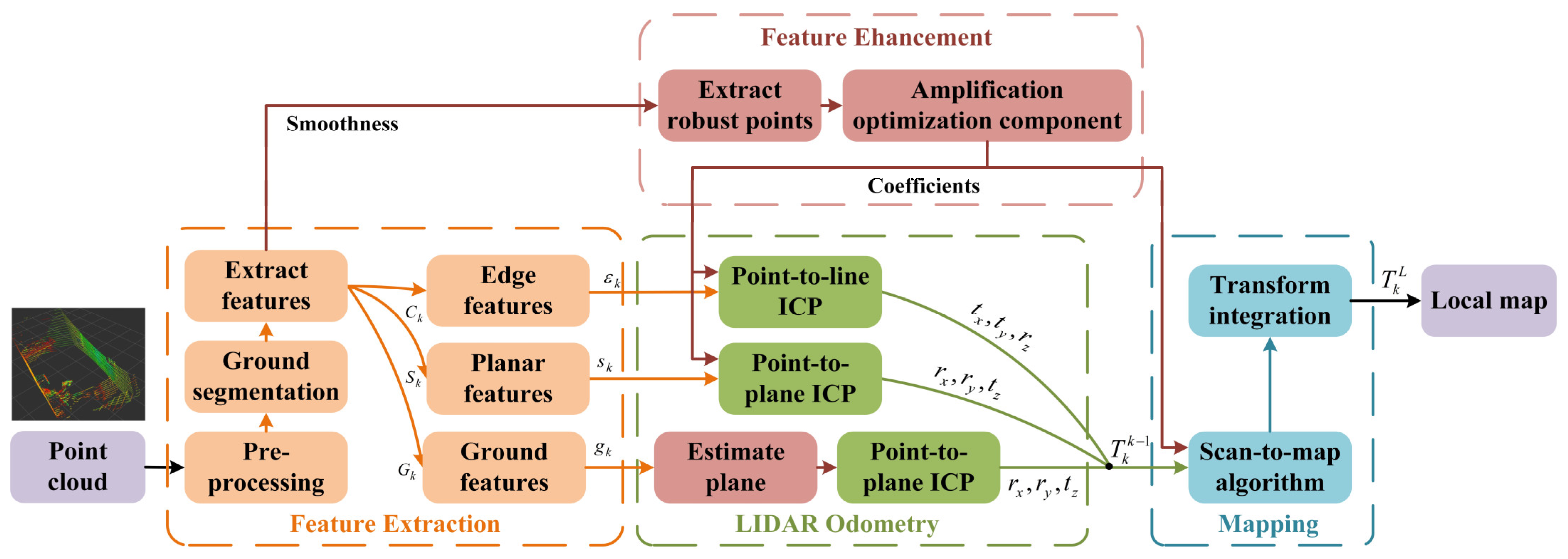
3.1. System Overview

The proposed feature-enhanced LiDAR SLAM system follows the standard pipeline of conventional LiDAR-based SLAM, consisting of feature extraction, odometry estimation, and map construction. On top of this architecture, a feature enhancement module is integrated to improve robustness and accuracy in complex environments.

As illustrated in Figure 1, the system first divides each LiDAR frame P_k into ground point cloud G_k and non-ground point cloud C_k. In the feature extraction module, edge feature points ε_k and planar feature points s_k are extracted from C_k, while ground feature points g_k are derived from G_k. These extracted features are then used to establish correspondences for both scan-to-scan and scan-to-map registration, thus forming geometric constraints that are solved by the optimizer to estimate the current frame’s pose.

To improve the reliability of feature matching and the accuracy of pose estimation, a stability-based feature enhancement module is introduced. Stable feature points are identified by analyzing the local distribution of smoothness scores derived from the feature extraction. During the optimization stage, an adaptive weighting strategy assigns greater influence to more stable features, thereby suppressing the impact of unreliable residuals. Additionally, for ground features, the system replaces traditional point-to-point associations with a locally fitted planar model, enhancing the spatial consistency of ground constraints. Finally, transformation estimates from different types of feature correspondences are fused to compute odometry poses, which are subsequently used to incrementally construct a dense and accurate map of the environment.

The proposed feature enhancement module is lightweight, as it fully reutilizes geometric features extracted by the baseline SLAM pipeline without incorporating any additional sensors, deep learning models, or high-dimensional feature descriptors. Instead, the enhancement strategy operates on low-cost statistical measures for evaluating feature stability and adaptively reweighting residuals. A detailed runtime comparison is provided in Section 4.3 to demonstrate the computational efficiency of the proposed system.

3.2. Point Cloud Preprocessing

In the preprocessing stage, a classical scan-line segmentation method inspired by LOAM is employed. The input point cloud is first transformed from Cartesian to polar coordinates. Based on the intrinsic angular parameters of the LiDAR sensor, each point is assigned a corresponding scan line index. Points that exceed the expected angular resolution are regarded as environmental noise and subsequently removed.

To facilitate efficient ground segmentation, a spherical projection-based point cloud mapping strategy [41,42] is adopted. The raw 3D point cloud captured by the LiDAR is projected onto a depth image, providing a structured and compact representation. Each point $p_i=\left(x,y,z\right)\in {ℝ}^3$ is projected onto the 2D image space $\left(u,v\right)\in {ℝ}^2$ is defined as follows:

$$\left(\begin{array}{c}u\\ v\end{array}\right)=\left(\begin{array}{c}1/2\left[1-\arctan \left(y,x\right){\pi }^{-1}\right]\omega \\ \left[1-\left(\arcsin (z{r}^{-1})+f_{up}\right)f^{-1}\right]h\end{array}\right)$$

(1)

where $\omega$ and $h$ denote the width and height of the depth image, respectively, and $r=\sqrt{x^2+y^2+z^2}$ represents the range of the point in polar coordinates. The vertical field of view (FOV) of the LiDAR is defined as $f$.

Given the characteristics of LiDAR data—sparse vertical and dense horizontal resolution—the depth image height is set to the number of scan lines, while the width is appropriately compressed to reduce redundancy.

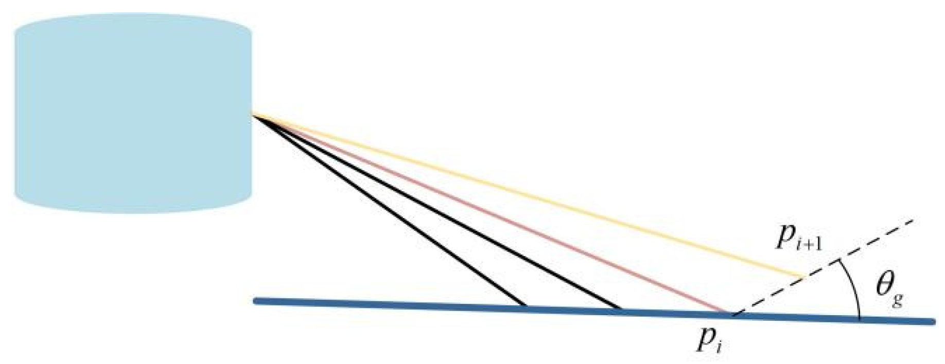
3.3. Ground Segmentation

Based on the constructed depth image, ground segmentation is performed, following the approach in [11,43]. The lower region of the depth image typically corresponds to the ground surface due to the sensor’s perspective. As illustrated in Figure 2, ground points are identified by analyzing the geometric relationship between adjacent pixels along vertical scan lines.

Given two vertically adjacent points $p_i(x_i,y_i,z_i)$ and $p_{i+1}(x_{i+1},y_{i+1},z_{i+1})$, their local difference vector is computed as $p_{i+1}-p_i=\left(\Delta x,\Delta y,\Delta z\right)$. The inclination angle ${\theta }_g$ between this vector and the horizontal plane is then calculated as:

$${\theta }_g=\arctan \left({\displaystyle \frac{\Delta z}{\sqrt{\Delta x^2+\Delta y^2}}}\right)$$

(2)

If the angle difference is $\left|{\theta }_g-{\theta }_m\right|<{\tau }_{\theta }$, the region is classified as ground and marked, where ${\theta }_m$ denotes the sensor’s mounting pitch angle.

The ground mask is generated through the following procedure:

A matrix $G\in {\left\{-1,0,1\right\}}^{\omega \times h}$ is initialized, where all entries are set to −1, indicating invalid or occluded regions. A vertical search range $[0,{\omega }_g]$ is defined, where ${\omega }_g$ corresponds to a fixed number of rows at the bottom of the image. For each valid pixel $(u,v)$, within this region, the angle ${\theta }_g$ with its vertically adjacent pixel $(u+1,v)$ is computed. If the condition is satisfied, both $G\left(u,v\right)$ and $G\left(u+1,v\right)$ are marked as 1 (ground); otherwise, the current pixel is marked as 0. If either pixel is invalid, $G\left(u,v\right)$ remains −1.

After the mask is generated, all pixels labeled as ground are projected back into 3D space to form the ground point set:

$$G_k=\left\{p_i|G\left(u,v\right)=1\right\}$$

(3)

3.4. Feature Extraction

During the feature extraction stage, salient geometric structures are identified based on the smoothness scores of the point cloud. The smoothness score [10] effectively captures local geometric variations and is widely used for detecting edge and planar features. For non-ground points, the local smoothness for a point is computed as:

$$c_i={\displaystyle \frac{1}{\left|W\right|}}{\displaystyle \sum }_{j\in W,j\ne i}\left(p_j\left(x,y,z\right)-p_i\left(x,y,z\right)\right)$$

(4)

where $p_i$ denotes the i-th point in the current scan $P$, and $W$ is a local neighborhood comprising 10 adjacent points along the same scan ring, with $p_i$ at the center.

In each scan frame, all points are sorted according to their smoothness scores $c_i$. Points with high $c_i$ values are selected as edge features, while those with low $c_i$ are classified as planar features.

For ground points, since their geometric variations primarily occur along the horizontal directions (i.e., the X and Y axes in the LiDAR coordinate frame), the smoothness score is computed using only the horizontal components:

$$c_i^g={\displaystyle \frac{1}{\left|W\right|}}‖{\displaystyle \sum _{j\in W,j\ne i}(p_j(x,y)-p_i(x,y))}‖$$

(5)

3.5. Stable Feature Point Selection

To further select stable feature points from the initially extracted candidates, a two-pronged selection mechanism is introduced that targets both intra-frame and inter-frame stability. The goal is to identify feature points that exhibit strong structural consistency and temporal observability, as illustrated in Figure 3.

This method is inspired by the Normal Distributions Transform (NDT) [44,45,46], but unlike NDT—which models the spatial distribution of points using Gaussian representations—the proposed method focuses on modeling the statistical distribution of local smoothness scores. In environments with irregular structures or significant density variation, spatial point distributions are often insufficient to reliably reflect physical consistency. In contrast, our work models the distribution of local surface smoothness—an attribute that more directly captures the geometric variation within neighborhoods.

Smoothness scores, as differential descriptors of local geometric change, exhibit statistically predictable behavior in regions with continuous and stable topological structures. When evaluated over appropriate spatial scales, the statistical distribution of smoothness scores provides an effective indicator of inherent structural characteristics, enabling the selective enhancement of high-quality feature points.

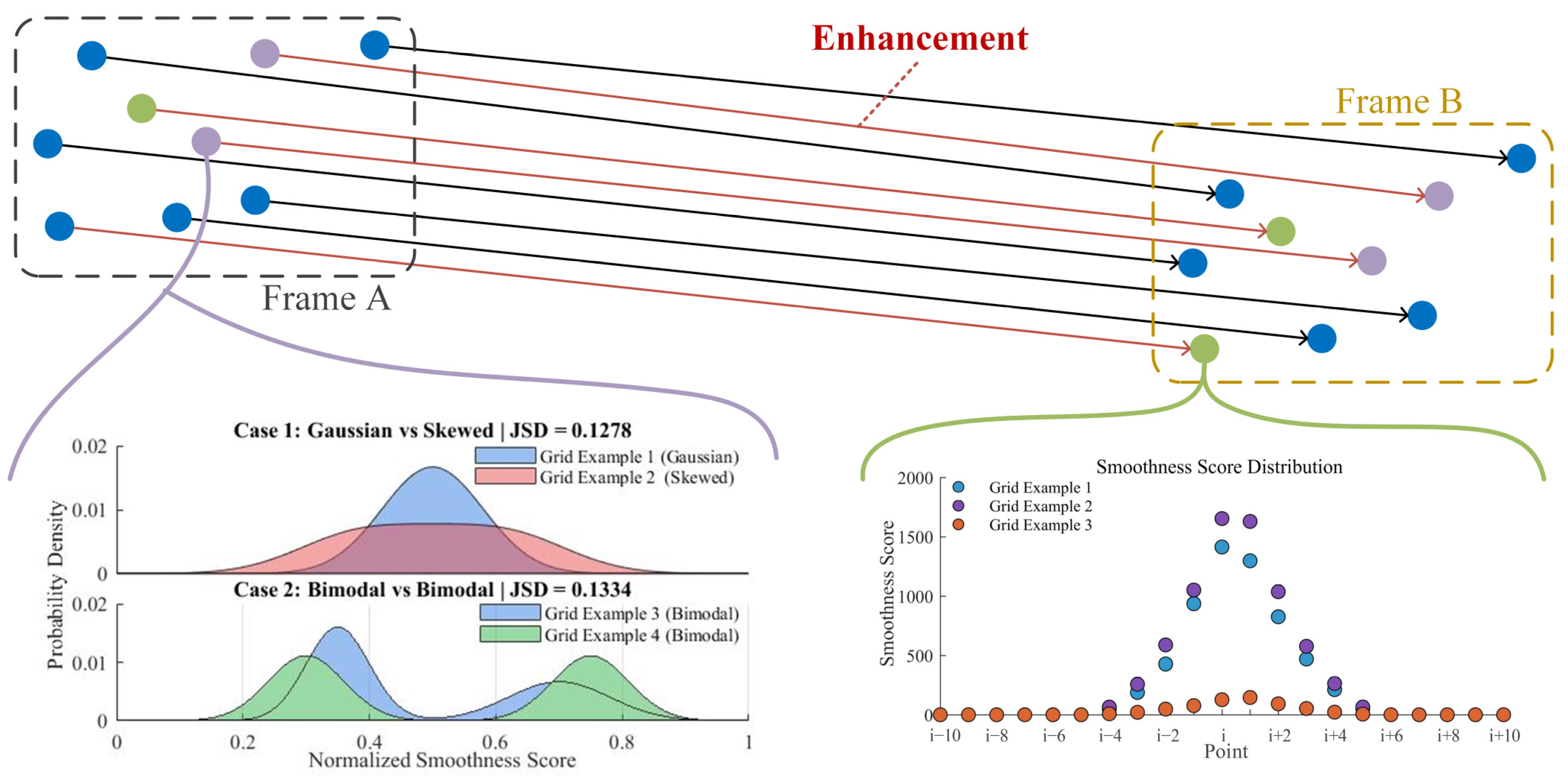
3.5.1. Spatially Stable Feature Point Selection

To identify structurally stable feature points within each frame, a spatial selection strategy is proposed based on the statistical characteristics of local smoothness. Regions exhibiting statistically regular distributions of smoothness scores are identified using normality tests, as such patterns often correspond to geometrically regular and topologically stable surfaces.

In implementation, we design an efficient selection pipeline that integrates scan-line topology with statistical inference. For each candidate feature point, a local neighborhood is extracted along the LiDAR scan line and the region is discretized into one-dimensional (1D) grid cells of size 20 × 1. Compared to traditional 3D voxel partitioning schemes (e.g., as used in NDT), this 1D segmentation is better aligned with the LiDAR’s data acquisition pattern and significantly improves computational efficiency. Each grid cell reuses precomputed smoothness scores, thereby avoiding redundant calculations.

To evaluate the statistical regularity within each cell, the Shapiro–Wilk normality test is employed. The test statistic is defined as:

$$S_t={\displaystyle \frac{{\left({\displaystyle {\sum }_{i=1}^n{a}_i{c}_{(i)}}\right)}^2}{{\displaystyle {\sum }_{i=1}^n{(c_i-\overline{c})}^2}}}$$

(6)

where $a_i$ denotes the normality test coefficient, $c_{(i)}$ is the i-th order statistic of smoothness scores, and $\overline{c}$ is their sample mean. A grid is considered to approximately follow a normal distribution if $S_t$ exceeds a predefined threshold $\lambda$.

For grids that pass the normality test, the mean $\mu$ and standard deviation $\sigma$ of smoothness are calculated. The feature points within the interval $\left[\mu -\sigma ,\mu +\sigma \right]$ are selected and labeled as spatially stable.

3.5.2. Temporal Stable Feature Point Selection

While spatial modeling effectively captures local structural regularity within a single frame, ensuring temporal consistency is equally important for reliable feature association across consecutive scans. To enhance the robustness of inter-frame matching, we introduce a statistical consistency metric based on the Jensen–Shannon Divergence (JSD), which quantifies the structural variation between corresponding regions across frames.

Unlike methods that rely on specific distributional assumptions, JSD offers a non-parametric measure of similarity between two probability distributions, thereby serving as a general indicator of statistical consistency.

During registration, a histogram of smoothness scores is constructed for each feature point’s surrounding grid cell in the current frame (denoted as $D_P$), and is compared to the corresponding cell $D_Q$ from the aligned region in the reference frame. The JSD between $D_P$ and $D_Q$ is computed as:

$$D_{JS}(D_P\Vert D_Q)={\displaystyle \frac{1}{2}}{D}_{KL}(D_P\Vert M)+{\displaystyle \frac{1}{2}}{D}_{KL}(D_Q\Vert M)$$

(7)

where $M=1/2(D_P+D_Q)$, and $D_{KL}(\cdot |\cdot )$ denotes the Kullback–Leibler divergence. If $D_{JS}<\tau$, the region is considered temporally consistent, and the corresponding feature point is assigned a temporal stability label.

Both the Shapiro–Wilk test and the Jensen–Shannon divergence are computationally lightweight, making them well-suited for real-time integration in LiDAR registration pipelines.

3.6. Feature Association

Following the extraction of edge, planar, and ground features, the system constructs geometric associations among them to establish residual constraints. To accommodate the distinct geometric properties of different feature types, the system employs feature-specific association strategies. Edge features are aligned via point-to-line associations, planar features via point-to-plane associations, and ground features are associated with a globally fitted ground plane via orthogonal projection, instead of relying on traditional local point-to-plane matching.

These residuals are then minimized through the Iterative Closest Point (ICP) registration process between two point clouds $P_k$ and $P_{k-1}$ to estimate the relative pose transformation $T_k^{k-1}$, which serves as the foundation of the LiDAR odometry pipeline.

It is worth noting that these associations are established over the feature sets extracted in Section 3.4. The stability assessment introduced in Section 3.5 is incorporated later in Section 3.7 to assign adaptive confidence weights, thereby modulating each feature’s contribution during the optimization process.

3.6.1. Edge and Planar Feature Associations

For each edge feature point $p_i^{{\epsilon }_k}\in P_k$, two nearest non-collinear edge points $P_{n1}^{{\epsilon }_{k-1}}$ and $P_{n2}^{{\epsilon }_{k-1}}$ are selected from the previous scan $P_{k-1}$ to construct a point-to-line residual. The Euclidean residual is defined as:

$$d_i^{\epsilon }={\displaystyle \frac{‖(p_i^{{\epsilon }_k}-p_{\mathrm{n}1}^{{\epsilon }_{k-1}})\times (p_i^{{\epsilon }_k}-p_{n2}^{{\epsilon }_{k-1}})‖}{‖p_{n1}^{{\epsilon }_{k-1}}-p_{n2}^{{\epsilon }_{k-1}}‖}}$$

(8)

This residual quantifies the orthogonal distance from the current point to the line defined by its two nearest neighbors in the previous frame.

For each planar features $p_i^{s_k}\in P_k$, three nearest non-coplanar points $P_{n1}^{s_{k-1}}$, $P_{n2}^{s_{k-1}}$ and $P_{n3}^{s_{k-1}}$ are selected from the previous scan $P_{k-1}$. The point-to-plane residual is formulated as:

$$d_i^s={\displaystyle \frac{‖(p_i^{s_k}-p_{n1}^{s_{k-1}})\cdot (p_{n1}^{s_{k-1}}-p_{n2}^{s_{k-1}})\times (p_{n1}^{s_{k-1}}-p_{n3}^{s_{k-1}})‖}{‖(p_{n1}^{s_{k-1}}-p_{n3}^{s_{k-1}})\times (p_{n2}^{s_{k-1}}-p_{n3}^{s_{k-1}})‖}}$$

(9)

where $P_{n1}^{s_{k-1}}$, $P_{n2}^{s_{k-1}}$ and $P_{n3}^{s_{k-1}}$ must lie on different scan lines to avoid geometric degeneration.

3.6.2. Ground Feature Association

Ground feature association is performed using a strategy based on a globally fitted planar model. This approach enforces stronger structural constraints on the ground region by suppressing the influence of outliers and isolated noise points, thereby enhancing the overall consistency of the ground-related residuals. Essentially, this residual model extends the conventional ICP point-to-plane formulation.

Considering the non-uniform spatial distribution of LiDAR point clouds—where point density decreases with distance and susceptibility to external disturbances increases—the system excludes ground points beyond 50 m before model fitting. Only nearby, high-confidence points are retained to reduce data scale and mitigate the impact of noisy measurements.

Subsequently, the ground plane is then estimated using RANSAC on a subset of ground-labeled points from the registration frames. For the ground feature point $p_i^{g_k}\in P_k$, the estimated plane is expressed as:

$$n_g^{k-1}\cdot p_i^{g_{k-1}}+D=0$$

(10)

where the resulting plane normal $n_g^{k-1}=(A,B,C)$ serves as a critical parameter for constructing geometric constraints. Ground feature points from the current scan are then orthogonally projected onto the fitted plane, and the residual for each point is computed as its perpendicular distance to the surface:

$$d_i^g={\displaystyle \frac{\left|p_i^{g_k}\cdot n_g^{k-1}+D\right|}{\left|n_g^{k-1}\right|}}$$

(11)

3.7. Stability-Aware Feature Enhancement Weighting

After constructing the geometric residuals, an adaptive weighting strategy is applied to incorporate feature stability into the pose estimation process. This mechanism dynamically adjusts the contribution of each residual based on the spatial (intra-frame) and temporal (inter-frame) stability of the associated feature, thereby enhancing the influence of structurally reliable observations during optimization.

For intra-frame stable feature points, stability is evaluated based on the smoothness gradient $\nabla c$ within each grid cell. Features located in stable regions are assigned weights according to:

$${\omega }_s=u_s\cdot \sigma (‖\nabla c‖)$$

(12)

where $u_s$ is an empirically determined spatial enhancement factor that controls the baseline influence of stable features within a frame. The sigmoid function $\sigma (x)=1/(1+e^{-kx})$ ensures smooth and bounded modulation of weights, preventing excessive amplification in high-gradient regions.

For inter-frame stability, the Jensen–Shannon Divergence (JSD) between the curvature distributions of corresponding regions across consecutive scans is used to quantify temporal consistency. A temporal weighting factor is defined as:

$${\omega }_k=u_k\cdot \sigma (\tau -D_{JS})$$

(13)

where $u_k$ is an empirically defined temporal enhancement factor, and $\tau$ is a fixed threshold that defines the response center of the sigmoid function, controlling the sensitivity of weight decay in response to inter-frame divergence. When the JSD $D_{JS}$ is small, indicating consistency across frames, the weight ${\omega }_k$ approaches $u_k$, thereby increasing the contribution of temporally stable features.

The final enhancement weight ${\omega }_e$ is calculated as:

$${\omega }_e=\min (\max ({\omega }_1,{\omega }_2)+\alpha \min ({\omega }_1,{\omega }_2),1)$$

(14)

where $\alpha$ is an additional gain coefficient for joint spatiotemporal enhancement.

The complete pose estimation process is formulated as a unified non-linear optimization objective:

$$T^{*}=\arg \underset{T}{\min }\left({\displaystyle \sum {\omega }_e\cdot ‖d_i^{\epsilon }‖+{\displaystyle \sum {\omega }_e\cdot ‖d_i^s‖+}{\displaystyle \sum ‖d_i^g‖}}\right)$$

(15)

where $d_i^{\epsilon }$, $d_i^s$ and $d_i^g$ denote the point-to-line, point-to-plane, and ground-to-plane residuals respectively, corresponding to edge, planar, and ground features. Each residual is weighted by a stability-aware factor ${\omega }_e$, derived from the spatial and temporal consistency of the associated feature.

The proposed stability-aware mechanism is seamlessly integrated into conventional LiDAR SLAM pipelines. A two-stage Levenberg–Marquardt algorithm is employed for non-linear optimization in both scan-to-scan and scan-to-map registration. By incorporating feature-stability-weighted residuals, the method constructs a unified optimization objective that improves pose estimation accuracy while preserving computational efficiency. This design ensures compatibility with traditional SLAM frameworks without requiring structural modifications to existing system architectures.

4. Experiment

To qualitatively and quantitatively evaluate the proposed LiDAR-only SLAM framework, we performed a series of experiments using two representative datasets: the publicly available KITTI [47] and M2DGR [47] datasets. These datasets encompass diverse indoor and outdoor environments and serve as established benchmarks for autonomous driving and mobile robotics research.

The KITTI dataset contains LiDAR point clouds captured in urban and suburban environments using a Velodyne HDL-64E sensor. In contrast, the M2DGR dataset comprises a large-scale multi-environment collection captured by a ground robot equipped with a full sensor suite, including a Velodyne HDL-32C LiDAR. It features both indoor and outdoor segments, making it particularly challenging for SLAM algorithms. Previous studies have reported significant performance degradation on M2DGR [48], especially in scenes with densely vegetated outdoor paths, reflective glass walls, and long, textureless indoor corridors. Owing to these characteristics, the M2DGR dataset has in recent years become increasingly adopted for evaluating SLAM performance in complex [49,50,51], unstructured [52,53], and challenging environments [54,55,56].

We compared the proposed method with several widely recognized baselines and open-source SLAM systems under various real-world scenarios. Both qualitative trajectory visualizations and quantitative pose estimation metrics were used to evaluate the effectiveness of the proposed feature enhancement strategy. All experiments were conducted on an industrial-grade PC equipped with an Intel i7-10700 CPU, running Ubuntu 18.04 and the ROS Melodic framework.

4.1. Comparison with Baseline Algorithm

To validate the effectiveness of the proposed method, we conducted comparative experiments against the baseline algorithm LeGO-LOAM across multiple scenes. LeGO-LOAM, a classical LiDAR-based SLAM system, also served as the base framework upon which our enhancement modules were integrated.

4.1.1. Subjective Map Quality Comparison

The qualitative comparison on the M2DGR dataset confirms the effectiveness of the proposed approach. As shown in Figure 4, our method achieved consistent localization and mapping performance throughout the sequence, without noticeable registration errors, outperforming LeGO-LOAM in overall accuracy.

Figure 4 illustrates the comparative mapping results in four representative indoor and outdoor scenarios from the M2DGR dataset, including indoor environments (e.g., rooms and corridors), outdoor scenes with dense vegetation, and rotational or linear motion sequences.

In indoor scenarios, both methods successfully performed mapping and localization due to the regular distribution of geometric features, which supported stable SLAM operation. The reconstructed point cloud maps from both systems clearly depict wall contours and object boundaries in top-down views.

In contrast, in outdoor scenarios with dense vegetation and a lack of rigid structural elements, LeGO-LOAM suffered from significant performance degradation. The algorithm tended to extract predominantly unstable features, which were insufficient for reliable registration.

By comparison, our proposed method demonstrated significantly improved robustness and accuracy under such challenging conditions. This improvement stems from the integration of the stability-aware enhancement strategy, which emphasizes the contribution of reliable features during registration, enabling more consistent and accurate pose estimation.

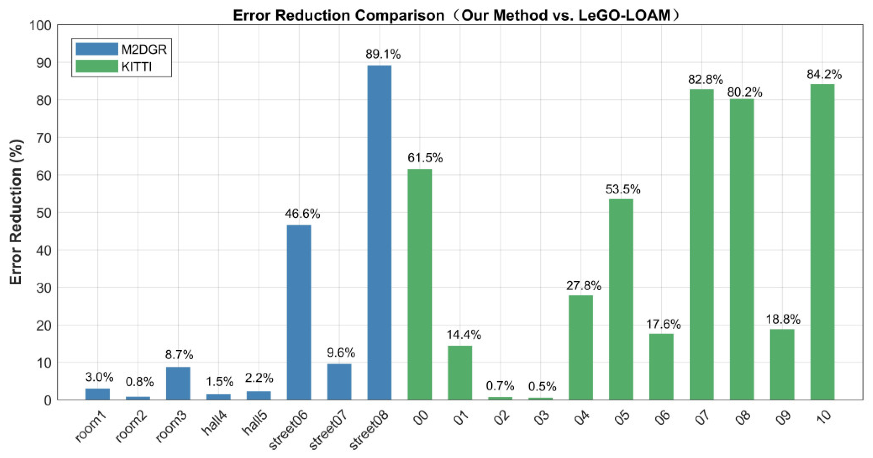
4.1.2. Objective Evaluation

To quantitatively evaluate the performance of the proposed method, the Root Mean Square Error (RMSE) of Absolute Trajectory Error (ATE) [57,58] was adopted as the primary metric (unit: meters). This widely used metric reflects the average deviation between the estimated trajectory and the ground-truth trajectory after alignment, and is computed as:

$$RMS{E}_{ATE}=\sqrt{{\displaystyle \frac{1}{n}}{\displaystyle \sum _{k=1}^n{(T_k^e-T_k^g)}^2}}$$

(16)

where $n$ is the number of poses, $T_k^e$ and $T_k^g$ denote the k-th estimated and ground-truth poses, respectively.

Table 1. RMSE ATE comparison with baseline on M2DGR dataset (unit: meters).

Seq.	Scene Type	LeGO-LOAM	Ours	Error Reduction
room1	Indoor–Room	0.1539	0.1493	2.99%
room2	Indoor–Room	0.1303	0.1293	0.77%
room3	Indoor–Room	0.1615	0.1474	8.73%
hall4	Indoor–Corridor	0.9304	0.9162	1.53%
hall5	Indoor–Corridor	0.9161	0.8958	2.22%
street06	Outdoor–Road	0.8119	0.4338	46.57%
street07	Outdoor–Road	3.1782	2.8748	9.55%
street08	Outdoor–Road	1.3677	0.1488	89.12%

Bold values denote the lowest error in each row.

presents the RMSE results of the proposed method compared with the baseline LeGO-LOAM across various indoor and outdoor sequences (abbreviated as “Seq.”) in the M2DGR dataset. In indoor environments, such as room1-room3 and hall4-hall5, both algorithms exhibited comparable performance, as the abundance of well-distributed geometric features facilitated reliable feature extraction and registration. Under these conditions, our method provided modest yet consistent improvements, reducing RMSE by an average of 3.25%.

It is important to emphasize that these seemingly modest gains in well-structured environments are still significant. They indicate that our method successfully refines the feature utilization process even when the baseline, leveraging abundant and reliable features inherent to such settings, is already performing near its theoretical upper bound. In other words, the relatively limited improvements should not be interpreted as negligible, but rather as a reflection of the diminishing returns typically encountered when attempting to further optimize performance in already well-conditioned environments.

However, in outdoor sequences (street06-street08), where the scenes were typically dominated by unstructured layouts, dense vegetation, and sparse rigid surfaces, the performance gap became significantly more pronounced. These environments posed challenges to point-based SLAM systems due to the prevalence of weak and unstable features, such as foliage and grass. LeGO-LOAM exhibited notable trajectory drift and localization failures, primarily due to the limitations of conventional feature extraction and registration strategies, which were not designed to handle unreliable or inconsistent features.

Critically, it is precisely in these complex scenarios that the core innovation of our method demonstrates its substantial value. By selectively amplifying the contribution of the limited pool of reliable observations, our approach achieves dramatic improvements where the baseline struggles profoundly. This resulted in an average RMSE reduction of 48.41% in outdoor scenarios, with the most significant improvement observed in street08, where the error was reduced by 89.12%. Overall, the average RMSE reduction was 20.19%. These findings clearly demonstrate the effectiveness of the proposed approach in extracting and utilizing stable features under challenging environmental conditions, while also providing consistent, valuable gains even in less demanding settings where the baseline framework is strong.

To further assess the generalizability of our method, we conducted experiments on the widely used KITTI dataset, which includes urban, suburban, and highway driving scenarios. As shown in

Table 2. RMSE ATE comparison with baseline on KITTI dataset (unit: meters).

Seq.	Scene Type	LeGO-LOAM	Ours	Error Reduction
00	Urban	5.9466	2.2901	61.48%
01	Highway	93.6190	80.1161	14.42%
02	Urban	56.8059	56.4135	0.69%
03	Rural	0.9121	0.9074	0.52%
04	Urban	0.3913	0.2824	27.81%
05	Urban	2.2142	1.0298	53.49%
06	Urban	0.9292	0.7655	17.61%
07	Urban	1.1430	0.1969	82.77%
08	Urban + Rural	3.8252	0.7570	80.21%
09	Urban + Rural	2.2011	1.7866	18.83%
10	Urban + Rural	2.2011	0.3488	84.15%

Bold values denote the lowest error in each row.

, our method consistently outperformed LeGO-LOAM across all sequences, achieving an average RMSE reduction of 40.18%. These results confirm the system’s capability to maintain precise localization in complex traffic environments characterized by frequent viewpoint changes, occlusions, and structural variations.

These improvements are further illustrated in Figure 5, which presents the relative improvement percentages achieved by our method across individual sequences in both the M2DGR and KITTI datasets. Each bar corresponds to a specific sequence, enabling a clear and concise comparison of performance gains across diverse environments. This visualization provides an intuitive overview of the distribution and magnitude of improvements, complementing the quantitative analysis in Table 1 and Table 2, and offering a clearer understanding of where and how the proposed method delivers its advantages.

Overall, the proposed method achieved an average RMSE reduction of 21.19% on the M2DGR dataset and 40.18% on the KITTI dataset, verifying its applicability across a wide range of real-world scenarios.

4.2. Comparison with Representative SLAM Systems

To further verify the effectiveness and robustness of the proposed method, we conducted comprehensive comparisons on the M2DGR dataset against several widely recognized and representative LiDAR-based SLAM systems, including LOAM, LeGO-LOAM, E-LOAM, and F-LOAM.

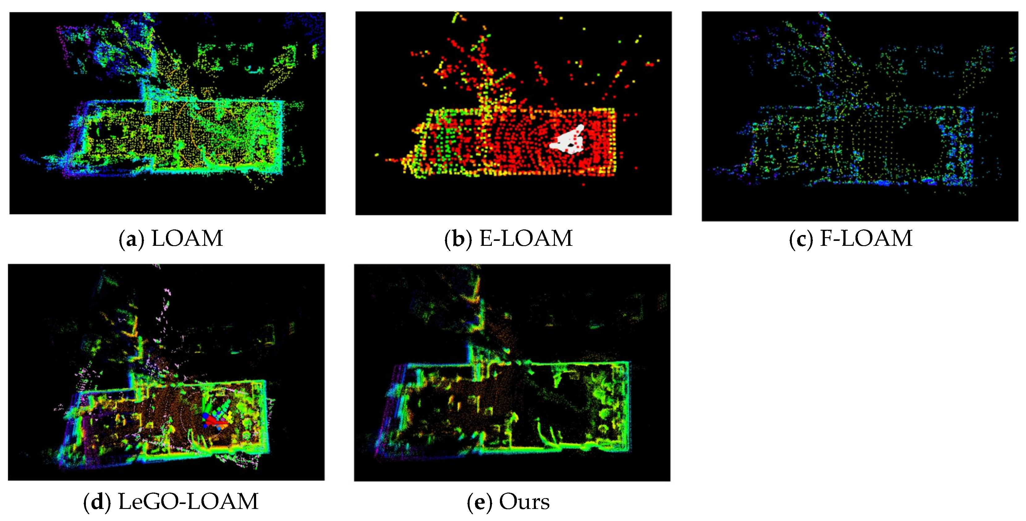
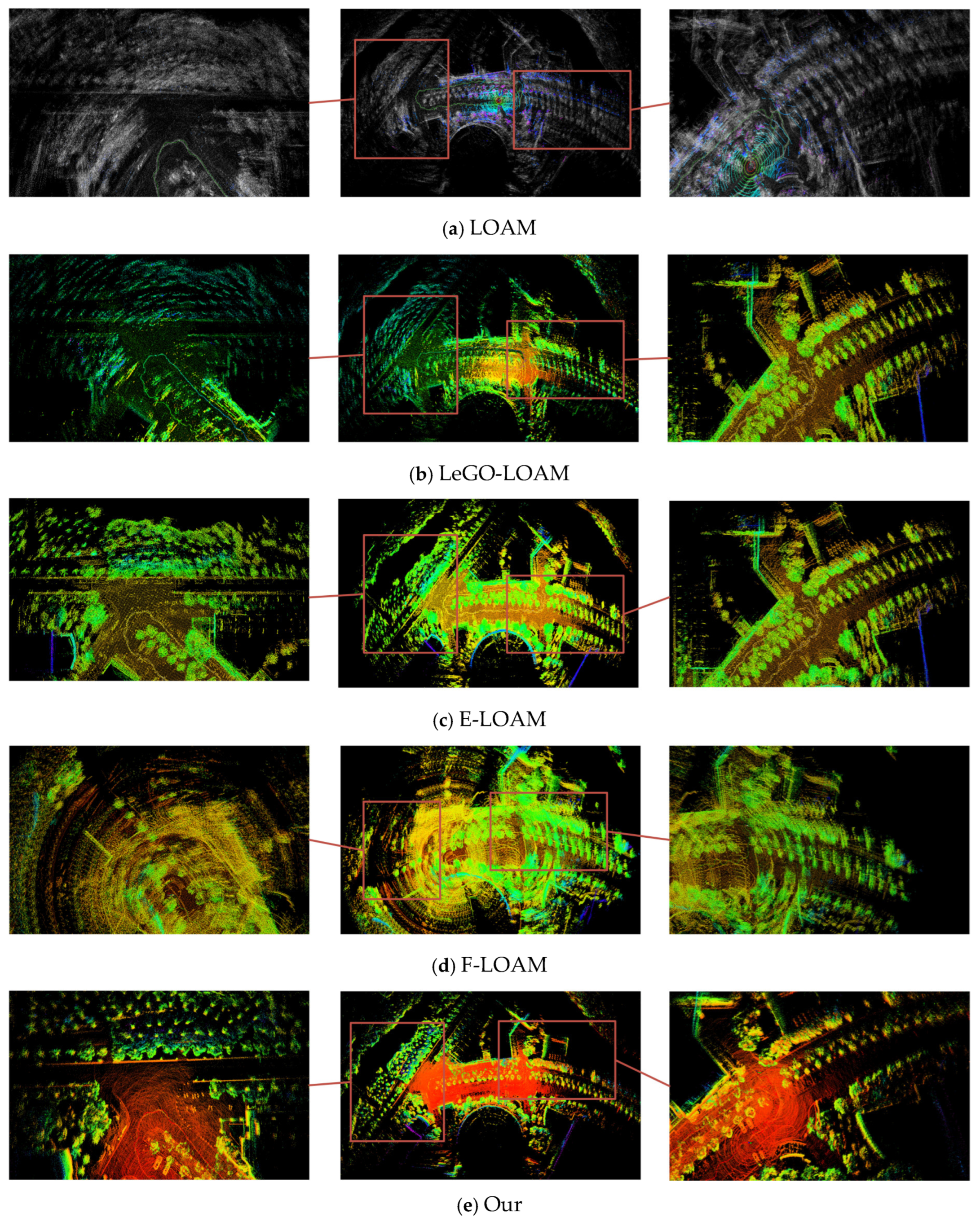
4.2.1. Subjective Map Quality Comparison

In the indoor sequences of the M2DGR dataset, where geometric features are dense and regularly distributed, all evaluated methods demonstrated robust localization and mapping performance. As illustrated in Figure 6, which presents mapping results in the room scenario, all SLAM systems produced high-quality maps with clear and complete reconstruction of wall contours and furniture layouts. The visual consistency among the outputs of different methods suggests that conventional LiDAR odometry pipelines are sufficient to ensure reliable performance in such environments, where the majority of feature points are stable and of high quality.

Furthermore, the trajectory error distributions in Figure 7 reveal that, although all methods performed well in structured indoor environments, the proposed method achieved more consistent and accurate pose estimation. The figure used color gradients to visualize the relative magnitude of trajectory errors across different frames, allowing intuitive comparisons among the methods.

For reference, the error ranges of LOAM, E-LOAM, F-LOAM, and LeGO-LOAM were 0.042–0.237 m, 0.083–0.887 m, 0.032–0.245 m, and 0.065–0.219 m, respectively. Notably, E-LOAM exhibits significant error spikes, with a maximum error reaching 0.887 m, indicating poor handling of unstable features in certain frames. While F-LOAM achieves the lowest minimum error, its upper bound remains high, suggesting less consistent performance across the sequence.

In contrast, the proposed method maintained an overall error range of 0.059–0.216 m, which was narrower than those of the other methods. This outcome highlights the effectiveness of the proposed stability-aware feature enhancement strategy in improving pose estimation accuracy. Moreover, the performance gain is not confined to isolated degraded frames but was consistently observed across the entire trajectory, resulting in a global and uniform improvement. This indicates that the system benefits not only in challenging moments but throughout all stages of operation, enhancing both local accuracy and overall trajectory consistency.

In complex and unstructured outdoor environments, where conventional SLAM systems often suffered from degraded performance, the proposed method delivered notably enhanced robustness and accuracy. As shown in Figure 8, which presents mapping results of a street scene adjacent to dense foliage, the generated point cloud maps are compared across methods, with zoomed-in regions provided on both the left and right sides to highlight geometric and structural details. The right side of the scene features a curved road flanked by regularly planted trees, where the geometric layout of road boundaries and adjacent building edges serves as a clear reference for identifying map distortion or misalignment. And the left side contains a hilly area with dense vegetation and natural terrain transitions, which provides a more challenging scenario for preserving fine-grained structural information. Ideally, a high-quality map in such environments should reveal crisp road boundaries, clear building contours without ghosting, and well-preserved vegetation structures. In the zoomed-in regions, tree arrangements should appear evenly spaced without duplication or elongation, and boundaries between man-made and natural structures should remain distinct and undistorted.

Among the baseline methods, LOAM, LeGO-LOAM, E-LOAM, and F-LOAM all exhibit varying degrees of degradation in these challenging regions. As seen in Figure 8, F-LOAM (Figure 8d) demonstrates the most severe deterioration, where trees along the road are significantly elongated or duplicated, and surrounding structures are distorted to the extent that the global layout becomes unrecognizable.

This severe deformation indicates substantial trajectory drift and registration failure. LOAM (Figure 8a) and LeGO-LOAM (Figure 8b) also showed significant issues. LOAM’s map suffers from indistinct vegetation and blurred edges, while LeGO-LOAM introduces circular distortions and unnatural structural warping, particularly in regions with unstructured backgrounds, such as dense vegetation and terrain transitions. E-LOAM (Figure 8c) performs slightly better but still exhibits noticeable boundary ambiguity and some misalignment in the vegetation structures. In the zoomed-in right-side views of these methods, trees along the road are stretched or doubled, indicating lateral drift and poor registration. In the left-side zoomed views, the vegetation structure becomes blurred or unnaturally distorted, with inconsistent density and noticeable ghosting effects.

These issues can be primarily attributed to the lack of stability assessment in conventional odometry pipelines. When unstable features—such as those from foliage, grass, or reflective surfaces—constituted a large proportion of the scene, the residual space became contaminated with high-noise or high-error terms. These unstable residuals affected the optimization process by introducing misleading or erroneous gradients, which resulted in inaccurate scan registration and degraded mapping performance.

In contrast, the proposed method integrated a dedicated feature stability evaluation and selection module, along with a stability-aware residual weighting mechanism. This design explicitly enhanced the influence of reliable features during scan registration. As evidenced in Figure 8e, our method achieves a geometrically consistent, structurally complete, and distortion-free point cloud map. Trees are preserved in proper alignment, building boundaries are sharp and ghost-free, and terrain transitions are clearly reconstructed. These qualitative observations also align with the objective evaluations presented in

Table 3. RMSE ATE Comparison with Representative methods on the M2DGR dataset (unit: meters).

Seq.	Scene Type	LOAM	LeGO-LOAM	F-LOAM	E-LOAM	Ours
room1	Indoor–Room	0.1567	0.1539	0.1608	0.2980	0.1493
room2	Indoor–Room	0.1324	0.1303	0.1336	0.1387	0.1293
room3	Indoor–Room	0.1597	0.1615	0.1659	0.3454	0.1474
hall4	Indoor–Corridor	0.9289	0.9304	0.9311	1.0243	0.9162
hall5	Indoor–Corridor	0.9013	0.9161	0.8978	0.9319	0.8958
street06	Outdoor–Road	0.5590	0.8119	0.9255	1.4031	0.4338
street07	Outdoor–Road	21.2160	9.2723	83.4078	3.2085	2.8748
street08	Outdoor–Road	0.5570	1.3677	50.1628	0.7543	0.1488

Bold values denote the lowest error in each row.

, where our method consistently achieves the lowest ATE RMSE across all sequences, confirming that improved localization directly contributes to higher-quality mapping outcomes.

The trajectory error distribution in Figure 9 further corroborates these findings. Since F-LOAM failed in the latter part of the sequence due to critical drift, it was excluded from the visualization. The heatmaps clearly show that all methods maintained low errors in straight-line segments, where the environment was relatively simple and the geometric structure was stable. However, in more complex areas—such as sharp turns and forested hill regions—the error increased dramatically. In these segments, LOAM, LeGO-LOAM, and E-LOAM exhibited pronounced error spikes, visualized as orange and red trajectories, indicating a lack of robustness to unstable or low-consistency features.

By contrast, the proposed method sustained low trajectory error throughout the entire sequence, even in high-risk and weakly structured regions. The consistent error control across variable environments further validates the effectiveness of the feature enhancement strategy in improving system robustness and maintaining accuracy under challenging conditions.

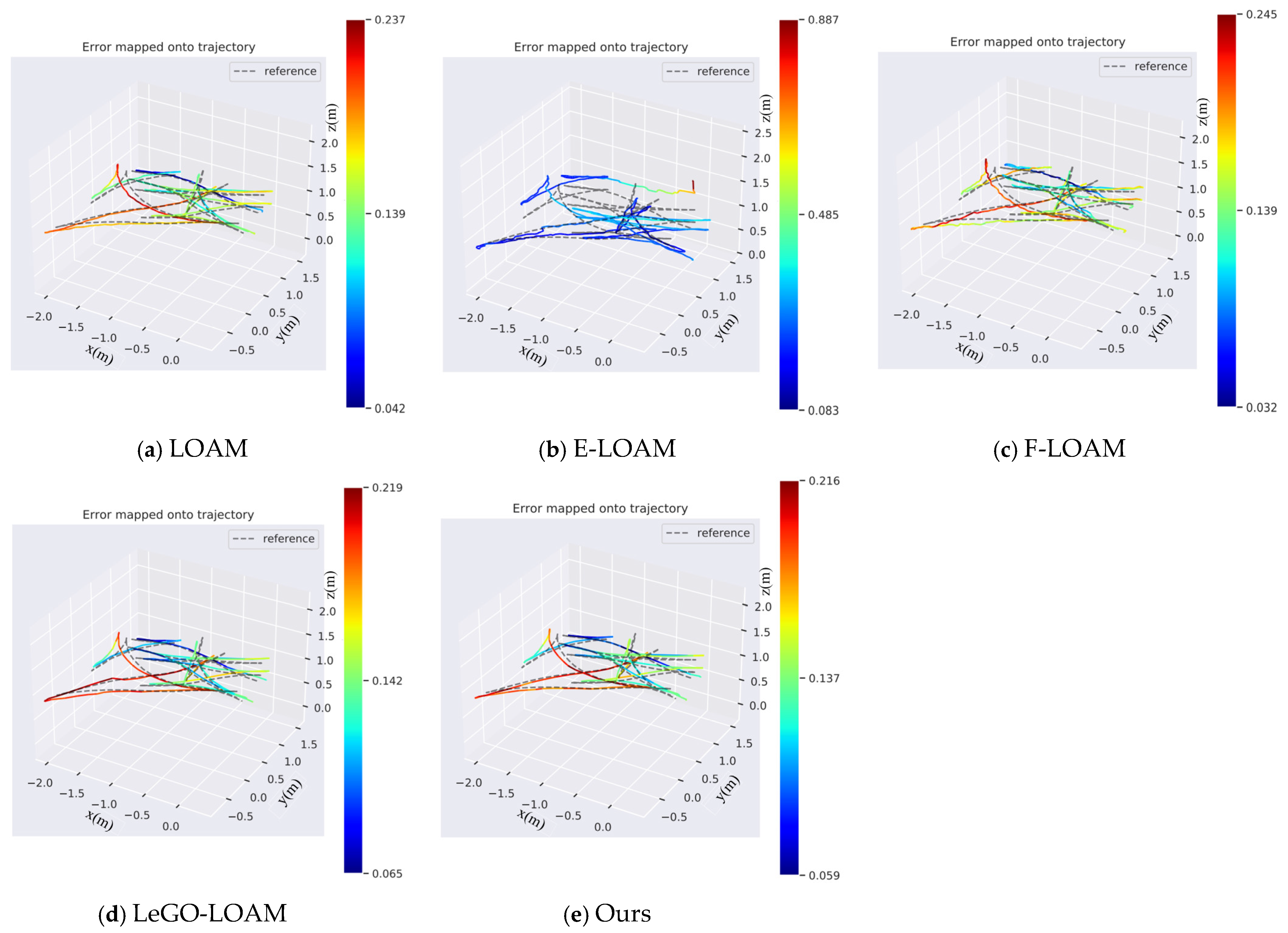
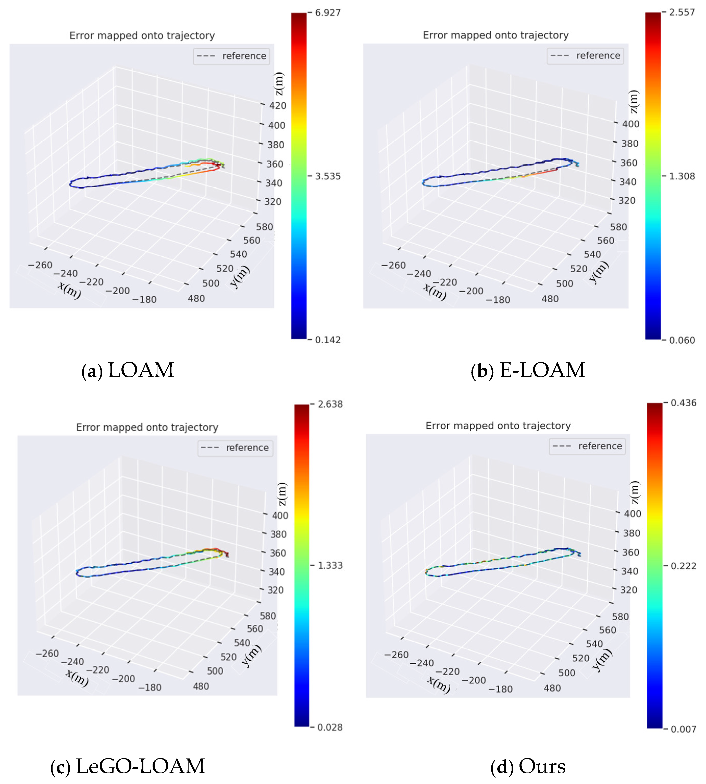
4.2.2. Objective Evaluation

To provide a more objective evaluation, we conducted quantitative experiments on both the challenging M2DGR dataset and the widely adopted KITTI dataset. The RMSE was also used as the primary metric to measure localization accuracy across different environments. Table 3 summarizes the results on M2DGR dataset, while

Table 4. RMSE ATE Comparison with Representative methods on the KITTI dataset (unit: meters).

Seq.	Scene Type	LOAM	LeGO-LOAM	F-LOAM	E-LOAM	Ours
00	Urban	2.4395	5.9466	4.7688	2.4943	2.2901
01	Highway	18.6474	93.6190	18.9226	264.6704	80.1161
02	Urban	117.1589	56.8059	8.5632	122.1116	56.413
03	Rural	0.9590	0.9121	0.9158	0.9533	0.9074
04	Urban	0.3889	0.3913	0.3618	33.3604	0.2824
05	Urban	2.4763	2.2142	3.4823	1.0605	1.0298
06	Urban	0.7676	0.9292	0.7906	0.7765	0.7655
07	Urban	0.5808	1.1430	0.6617	0.6738	0.1969
08	Urban + Rural	3.6795	3.8252	4.0830	4.9288	0.7570
09	Urban + Rural	1.7889	2.2011	1.8128	1.5503	1.7866
10	Urban + Rural	1.3463	2.201	1.4030	1.9565	0.3488

Bold values denote the lowest error in each row.

presents the results on KITTI dataset.

In indoor environments (e.g., room1–3 and hall4–5), all evaluated methods exhibited stable performance, which is consistent with the qualitative analysis. This relatively uniform performance can be primarily attributed to the structured nature of indoor scenes, which provide abundant and well-distributed geometric features that facilitate reliable feature extraction and accurate scan registration. However, our method can still achieve the lowest RMSE across most sequences, indicating that even in feature-rich scenarios, the proposed feature enhancement strategy consistently refines pose estimation by better leveraging high-quality observations.

In contrast, the performance gap became significantly more pronounced in unstructured outdoor environments, where traditional methods tend to degrade. These quantitative results further support the qualitative observations made earlier. For instance, in sequences street07 and street08, F-LOAM exhibited severe error accumulation, with RMSE values reaching 83.41 m and 50.16 m, respectively. According to conventional evaluation criteria in LiDAR SLAM, RMSE values exceeding 50 m are typically regarded as indicative of odometry failure. This aligns with the blurred and structurally ambiguous mapping results observed in Figure 8d, confirming the system’s inability to maintain reliable pose estimation under such conditions. This degradation can be attributed to the geometrically ambiguous nature of the environment, characterized by repetitive vegetation and the absence of salient planar or linear structures. In particular, the street07 sequence was collected along a zigzag route involving abrupt maneuvers, such as sharp turns, sudden braking, and rapid acceleration or deceleration [48], which, when coupled with the unstructured nature of the environment, resulted in highly irregular motion patterns that posed significant challenges for feature association. Consequently, F-LOAM, which relies on a sequential registration pipeline followed by distortion correction and refinement, is highly sensitive to unstable initial correspondences. Under such conditions, residuals become unreliable and rapidly diverge, leading to significant pose drift.

LeGO-LOAM, although comparatively more stable, still suffered from substantial drift, yielding errors of 9.27 m and 1.37 m. In comparison, the proposed method effectively reduced the RMSE to 2.87 m and 0.15 m, achieving relative improvements of 68.98% and 89.11% over LeGO-LOAM. Compared with LOAM (21.22 m and 0.56 m) and E-LOAM (3.21 m and 0.75 m), our method also achieved the lowest errors, outperforming LOAM by 86.47% and 73.21%, and E-LOAM by 10.53% and 80.13%, respectively. These results confirm that our approach delivers substantial benefits in non-structured and geometrically ambiguous environments, where conventional systems struggle due to unstable features and inconsistent residuals.

In contrast, the proposed method incorporates feature enhanced strategy that enables the identification of reliable features even in cluttered, low-observability environments. By explicitly enhancing the weights of stable features and down-weighting unreliable observations during optimization, the method effectively reduces the influence of erroneous residuals. This results in a more stable and well-conditioned residual space, along with more reliable gradient information, thereby enhancing the robustness of scan matching and enabling consistent trajectory estimation and high-quality map reconstruction in unstructured environments.

To further evaluate the generalization ability and adaptability of the proposed method in real-world traffic environments, we also conducted experiments on the widely adopted KITTI odometry benchmark. Table 4 presents the RMSE ATE results of our method and several representative SLAM baselines across 11 standard sequences.

As shown in Table 4, the proposed method consistently ranked among the top performers across all 11 standard sequences and achieved the lowest RMSE in nine sequences. Notable improvements are observed in sequences 00, 04, 07, 08, and 10, where our method reduced RMSE by over 70% compared to the weakest baselines, and by 10–40% relative to the strongest alternatives. In sequences 03, 05, 06, and 09, the proposed method also yields lower errors than the weakest baselines and marginally outperforms the best-performing methods, still achieving the lowest overall trajectory error. These sequences represent urban driving environments characterized by frequent viewpoint shifts, structural occlusions, and complex layouts. The superior results in these sequences validate the effectiveness of our stability-aware feature enhancement strategy in handling dense traffic scenes and complex spatial geometries.

Overall, the proposed method demonstrated consistently superior performance across a diverse range of environments, as confirmed by the quantitative evaluations presented in Table 3 and Table 4. On the M2DGR dataset, our method achieved the lowest RMSE ATE in all test sequences, encompassing both structured indoor areas and complex outdoor scenes. In relatively regular indoor settings, the proposed approach attained the most accurate trajectory estimations. In complex outdoor environments, the proposed approach exhibited even more pronounced advantages, effectively addressing the challenges posed by unstructured terrain.

As shown in Table 3 and Table 4, traditional SLAM systems, such as LOAM, LeGO-LOAM, and F-LOAM, frequently experienced significant performance degradation in scenes involving dense vegetation and unclear geometric structures. For instance, in sequences with vegetated street scenes, F-LOAM exhibited substantial drift, with final positional errors reaching up to 83.41 m, while LOAM encountered notable error spikes as large as 21.22 m. Even in relatively “easier” environments, traditional SLAM systems often cannot fully leverage high-quality features due to their reliance on rigid feature matching techniques. These methods do not adapt well to changes in the environment and often fail to account for dynamic or inconsistent feature distributions. The results obtained on the KITTI dataset further confirm the generalizability and effectiveness of our approach. In urban driving scenarios, where frequent viewpoint changes, occlusions, and sparse features are common, our method outperformed the baseline methods, demonstrating robust performance in complex, real-world environments.

The primary cause of this performance disparity is that traditional methods rely on fixed feature-matching rules and assign equal weight to every extracted feature, which limits their capacity to leverage the most reliable geometric cues and leads to suboptimal pose estimates even in relatively simple scenes. This gap becomes even more pronounced in unstructured terrains—such as vegetated hills or low-texture corridors—where scarce or unstable features introduce numerous low-quality observations into the registration pipeline. When unreliable correspondences dominate the residual space, noisy gradients distort the optimization landscape, often causing convergence to incorrect solutions or outright failure.

In comparison, our method addresses this challenge by placing more emphasis on stable features during optimization, effectively reducing the impact of low-quality observations. This approach leads to a more stable and accurate registration process, enabling our method to deliver more precise pose estimations and robust performance across a wide range of environments, even in less favorable conditions.

Nevertheless, our method consistently delivered superior performance across diverse scenarios by maximizing the utility of available observations. In structured, feature-rich environments, it effectively reinforced reliable observations, yielding incremental improvements even when baseline systems already perform well. In cluttered or weak-feature scenarios, this advantage became even more pronounced, where the method selectively amplifies stable features and suppresses noisy or unreliable ones, thereby significantly enhancing both robustness and localization accuracy. Such consistent performance across diverse environments makes the method particularly suitable for real-world deployment in both urban and off-road scenarios.

4.3. Runtime Performance Evaluation

To comprehensively assess the feasibility and runtime performance of the proposed method in practical deployments, we conducted time consumption comparisons on representative sequences in both indoor (M2DGR-room3) and outdoor (M2DGR-street08) scenarios. The evaluation included several widely adopted LiDAR odometry systems. All reported values represent the average processing time per frame, measured in milliseconds.

As summarized in

Table 5. Runtime Evaluation of LiDAR Odometry Methods (unit: ms).

Scenario	Stage	LOAM	E-LOAM	F-LOAM	LeGO-LOAM	Ours
	Feature Extraction	4.096	14.114	4.136	4.651	5.781
Indoor	Backend Optimization	21.641	65.472	41.207	1.292	1.037
	Total Odometry	25.737	79.586	45.343	5.943	6.818
	Feature Extraction	11.215	13.864	3.807	8.039	8.426
Outdoor	Backend Optimization	24.190	111.696	86.769	0.808	0.374
	Total Odometry	35.405	125.558	90.601	8.847	8.800

Bold values denote the lowest time consumption in each row.

, the proposed method demonstrates competitive runtime efficiency in both scenarios. In the indoor scenario, the total average odometry processing time is 6.818 ms, slightly higher than that of LeGO-LOAM (5.943 ms), but within the same order of magnitude. More importantly, it significantly reduces computational cost compared to conventional systems, such as LOAM (25.737 ms), F-LOAM (45.343 ms), and E-LOAM (79.586 ms), in terms of overall computational cost.

In the more challenging outdoor scenario, the proposed method achieves the lowest total processing time of 8.800 ms, slightly surpassing LeGO-LOAM (8.847 ms) and substantially outperforming the efficiency of LOAM (35.405 ms), F-LOAM (90.601 ms), and E-LOAM (125.558 ms). Notably, its pose optimization backend exhibits the lowest execution time among all evaluated systems.

This efficiency gain stems primarily from differences in feature processing and scan-matching strategies. Conventional systems, when faced with a high proportion of unstable or low-quality feature points, tend to construct a residual space laden with redundant or misleading constraints. This often leads to increased solver iterations and delayed convergence. In contrast, our method filters out unreliable observations and prioritizes high-confidence features, thereby reducing optimization complexity and accelerating convergence in pose estimation.

To further substantiate these findings, we analyzed the per-frame backend optimization time, as illustrated in Figure 10. Compared to LeGO-LOAM, our method not only maintains a lower average time per frame but also exhibits significantly reduced temporal variance. This indicates that the proposed approach consistently benefits from a well-conditioned and compact residual space across frames, enabling both fast and stable odometry computations.

Overall, the combination of per-frame efficiency and stability highlights the systemic benefits introduced by the proposed feature enhancement strategy. By emphasizing reliable features while suppressing unstable ones, the method improves the residual structure, facilitates faster solver convergence, and ultimately reduces the overall computational load.

5. Discussion

This Section presents an in-depth analysis of the proposed feature enhancement strategy. The method was systematically evaluated on two widely recognized LiDAR SLAM benchmarks, M2DGR and KITTI, using LiDAR sensors with varying resolutions, including the 32-beam and the 64-beam. Experimental results demonstrate consistent performance gains across diverse environments of the proposed strategy.

On the M2DGR dataset, which includes a variety of challenging indoor and outdoor scenes, the proposed method achieved the lowest RMSE ATE across all sequences when compared with representative SLAM methods. In structured indoor scenes, the method can further enhance performance over already well-performing conventional SLAM baselines. In generally unstructured outdoor environments, the performance gains become more pronounced. Quantitatively, the proposed method yielded an average RMSE reduction of 21.19% relative to the baseline pipeline. Evaluation on the KITTI odometry benchmark further substantiated these findings. Against a suite of representative SLAM algorithms, our method achieved the lowest RMSE ATE in 9 out of 11 standard sequences and realized an average reduction of 40.18% compared to the baseline pipeline. These results confirm the method’s strong generalization capabilities across a wide range of real-world scenarios.

Importantly, the proposed enhancement strategy is designed as a lightweight modular extension to conventional odometry pipelines, providing more reliable observations to the back-end optimization process. This “generic + enhanced” feature fusion framework achieves an effective trade-off between system adaptability and estimation accuracy, making the method well-suited for deployment in diverse and challenging real-world scenarios.

5.1. Smoothness-Based Feature Stability

The smoothness score serves as the central criterion in our stability-aware framework, providing a statistically grounded indicator of local geometric regularity. Compared to raw point coordinates, smoothness is a relative metric derived from the geometric relationships within a local neighborhood. It intrinsically reflects the curvature variation and geometric continuity between a point and its neighbors. These characteristics support for our feature enhancement strategy.

For spatial stability, empirical observations show that in well-structured and rigid regions, such as building facades, stationary vehicles, or poles, the smoothness scores within a local neighborhood tend to follow an approximately Gaussian distribution. This statistical regularity indicates the geometric stability of such rigid objects and suggests that the corresponding features remain consistent across frames, thereby offering high reliability for data association.

In contrast, unstructured or dynamic objects, such as trees, pedestrians, flags, or advertising banners, often undergo deformation or exhibit topological discontinuities. These factors lead to smoothness score distributions that are often skewed, multimodal, or heavy-tailed, deviating significantly from Gaussianity. Features in such regions tend to vary unpredictably over time and are more prone to noise and association errors.

It is important to note, however, that the inverse does not always hold true. Although well-structured objects often exhibit near-Gaussian smoothness distributions, approximate normality is not exclusive to them. In some unstructured environments, locally ordered and geometrically consistent subregions may exist where the smoothness scores exhibit near-Gaussian distributions. These subregions can be regarded as potentially structured features. Their localized geometric stability qualifies them as high-quality features, which contribute positively to point cloud registration. Accordingly, such features are included in our enhanced feature set under the same statistical stability criterion.

This observation can be visually illustrated in Figure 11, where spatially stable features identified by our method are highlighted in red. Notably, even in unstructured areas, such as the forested region on the left side of Figure 11b, the system successfully identifies stable points. As demonstrated in the downstream evaluation (e.g., Figure 8), enhancing such points contributes to measurable performance gains, especially in scenes where structural features are otherwise sparse. This capability is critical for improving robustness in weakly constrained scenarios and mitigating degradation due to feature sparsity.

Beyond spatial stability, the smoothness distribution across consecutive frames is also leveraged in our framework. The core idea is that if a region exhibits similar smoothness distributions over time, it is likely to maintain consistent local geometric structure. Conversely, large discrepancies in inter-frame smoothness distributions are indicative of dynamic disturbances or abrupt structural changes, suggesting lower reliability and a higher risk of introducing unstable residuals into the optimization process.

5.2. Threshold for Stable Feature Selection

The geometric stability (spatial dimension) and frame-to-frame stability (temporal dimension) of features are quantified through Shapiro–Wilk (SW) test and Jensen–Shannon Divergence (JSD), respectively. The determination of the thresholds combines statistical theoretical guidance with experimental optimization driven by data.

The Shapiro–Wilk test is employed to assess whether the data follows a normal distribution. The normality assumption is defined based on the Shapiro–Wilk test statistic, which ranges from 0 to 1. A value close to 1 indicates that the data is approximately normally distributed, while a value close to 0 indicates a low probability that the data meets the normal distribution assumption. The threshold of $\lambda >0.05$ is commonly used to determine if the data approximates a normal distribution, a standard widely accepted in statistical analysis [59,60,61]. In our practical data analysis, selecting 0.05 as the threshold effectively filtered out stable features, leading to reliable analysis results that ensured both odometry stability and accuracy.

In contrast to the Shapiro–Wilk test, Jensen–Shannon Divergence (JSD) lacks a universal, pre-defined threshold. JSD is commonly used to measure the similarity between two probability distributions and has widespread applications in fields, such as image detection [62,63] and point cloud processing [64,65]. In this study, we determined the JSD threshold based on insights from the work [66], which conducted a comparative analysis of the JSD distributions for the same objects viewed from different angles (reflecting intrinsic stability) and between different objects (reflecting dissimilarity). By analyzing the experimental data [66], we initially selected $\tau =0.2$ as the threshold and tested its neighborhood thresholds with a step size of 0.01 to assess the impact on the system’s overall pose estimation accuracy. The final optimal threshold was determined to be 0.18, as it effectively balanced the distinction between stable and unstable features.

Although we have employed an experimental threshold-setting approach in this work, which has yielded satisfactory results, future research will focus on exploring more flexible and automated threshold selection mechanisms to further improve the method’s adaptability and performance in diverse environments. The goal is to optimize the threshold through an automated fitting and dynamic adjustment strategy, where thresholds are adjusted based on the feature distribution of each frame and environmental changes, rather than relying on a globally fixed value. This approach is expected to not only enhance accuracy on a global scale but also allow adaptive adjustments for each frame, ensuring that feature registration for every frame is optimized.

5.3. Performance Boundaries and Application Potential

While the proposed method has demonstrated substantial improvements in a wide range of scenarios, its performance gains are ultimately constrained by the observability and quality of features extracted by the underlying front-end module. It is important to emphasize that the proposed approach is designed to optimize the utility of existing information, rather than generate new features. Therefore, in extremely sparse or weakly constrained scenes, the enhancement strategy reaches a natural upper bound in its contribution to pose estimation.

This limitation is clearly illustrated in Sequence 01 of the KITTI dataset, where in a highway scenario with extremely sparse feature points, both the baseline and the proposed method failed, as evidenced by the absolute trajectory error exceeding 80 m, which is typically considered a failure in localization. However, a quantitative analysis reveals an important distinction: even under this failure condition, our method still achieved a 14.42% relative accuracy improvement compared to the original baseline, as shown in Table 2.

This observation underscores the method’s fundamental limitation: the primary cause of performance degradation is not the failure of the feature enhancement mechanism, as it still provides a consistent improvement, but rather the inability of the front-end feature extractor to obtain a sufficient number of valid observations from the environment. As illustrated in Figure 12, the long, featureless road lacks significant structure, resulting in the number of feature points falling below the baseline system’s operational threshold. In such cases, the enhancement strategy can only slow down the performance degradation by improving the quality of the limited features, but it cannot fully address the problem of feature scarcity.

Thus, the feature enhancement method is most effective in structured scenes or in unstructured environments with a certain quantity of features, even if their quality is low. In environments where features are particularly sparse, the enhancement approach provides only limited improvements.

Additionally, the framework is computationally efficient and capable of real-time execution on conventional industrial PCs (e.g., Intel i7-10700) without requiring GPU acceleration. Notably, the integration of the feature enhancement module does not introduce significant computational overhead. On the contrary, by constructing a more consistent and well-conditioned residual space, the method facilitates faster convergence during back-end optimization, thereby indirectly improving runtime efficiency.

This lightweight design ensures compatibility with higher-level modules, such as semantic mapping, dynamic object filtering, or loop closure. Its practical deployability extends the applicability of the method in both academic research and industrial autonomous robotic systems.

6. Conclusions

This paper presents FE-LOAM, a lightweight and effective feature enhancement strategy for LiDAR odometry, designed to improve localization accuracy and robustness in complex and unstructured environments. The method introduces a stability-driven mechanism for identifying reliable non-ground features based on local smoothness distributions, and selectively reinforces their impact during pose optimization through adaptive residual weighting. For ground features, the algorithm replaces discrete point correspondences with fitted planar constraints, improving the consistency and robustness of ground registration.

Extensive experiments conducted on the KITTI and M2DGR datasets demonstrate that the proposed method consistently outperforms baseline approaches in both accuracy and robustness, while maintaining real-time performance. Compared with baseline methods, FE-LOAM achieves lower odometry drift, generates more complete and coherent point cloud maps, and significantly reduces computational spikes caused by unstable features. These results highlight the effectiveness and practicality of the proposed strategy for real-time LiDAR odometry in complex real-world applications.

References

1. Zhang, X.; Dong, J.; Zhang, Y.; Liu, Y.H. MS-SLAM: Memory-Efficient Visual SLAM with Sliding Window Map Sparsification. J. Field Robot. 2025, 42, 935–951. [Google Scholar] [CrossRef]
2. Zhu, F.; Zhao, Y.; Chen, Z.; Jiang, C.; Zhu, H.; Hu, X. DyGS-SLAM: Realistic Map Reconstruction in Dynamic Scenes Based on Double-Constrained Visual SLAM. Remote Sens. 2025, 17, 625. [Google Scholar] [CrossRef]
3. Huang, L.; Zhu, Z.; Yun, J.; Xu, M.; Liu, Y.; Sun, Y.; Hu, J.; Li, F. Semantic loopback detection method based on instance segmentation and visual SLAM in autonomous driving. IEEE Trans. Intell. Transp. Syst. 2024, 25, 3118–3127. [Google Scholar] [CrossRef]
4. Wang, S.; Song, A.; Miao, T.; Ji, Q.; Li, H. A LiDAR SLAM Based on Clustering Features and Constraint Separation. IEEE Trans. Instrum. Meas. 2025, 74, 1–18. [Google Scholar] [CrossRef]
5. Wang, J.; Xu, M.; Zhao, G.; Chen, Z. 3-D LiDAR Localization Based on Novel Nonlinear Optimization Method for Autonomous Ground Robot. IEEE Trans. Ind. Electron. 2024, 71, 2758–2768. [Google Scholar] [CrossRef]
6. Si, Y.; Han, W.; Yu, D.; Bao, B.; Duan, J.; Zhan, X.; Shi, T. MixedSCNet: LiDAR-Based Place Recognition Using Multi-Channel Scan Context Neural Network. Electronics 2024, 13, 406. [Google Scholar] [CrossRef]
7. He, Y.; Li, B.; Ruan, J.; Yu, A.; Hou, B. ZUST Campus: A lightweight and practical LiDAR SLAM dataset for autonomous driving scenarios. Electronics 2024, 13, 1341. [Google Scholar] [CrossRef]
8. Fujinaga, T. Autonomous navigation method for agricultural robots in high-bed cultivation environments. Comput. Electron. Agric. 2025, 231, 110001. [Google Scholar] [CrossRef]
9. McDermid, G.J.; Terenteva, I.; Chan, X.Y. Mapping Trails and Tracks in the Boreal Forest Using LiDAR and Convolutional Neural Networks. Remote Sens. 2025, 17, 1539. [Google Scholar] [CrossRef]
10. Zhang, J.; Singh, S. LOAM: Lidar odometry and mapping in real-time. In Proceedings of the Robotics: Science and Systems, Rome, Italy, 13–17 July 2015; RSS Foundation: Rome, Italy, 2014; Volume 2, pp. 1–9. [Google Scholar]
11. Shan, T.; Englot, B. LeGO-LOAM: Lightweight and ground-optimized LiDAR odometry and mapping on variable terrain. In Proceedings of the 2018 IEEE/RSJ International Conference on Intelligent Robots and Systems (IROS), Madrid, Spain, 1–5 October 2018; IEEE: Piscataway, NJ, USA, 2018; pp. 4758–4765. [Google Scholar]
12. Wang, Z.; Liu, G. Improved LeGO-LOAM method based on outlier points elimination. Measurement 2023, 214, 112767. [Google Scholar] [CrossRef]
13. Wang, Z.; Yang, L.; Gao, F.; Wang, L. FEVO-LOAM: Feature extraction and vertical optimized Lidar odometry and mapping. IEEE Robot. Autom. Lett. 2022, 7, 12086–12093. [Google Scholar] [CrossRef]
14. Liang, S.; Cao, Z.; Guan, P.; Wang, C.; Yu, J.; Wang, S. A novel sparse geometric 3-D LiDAR odometry approach. IEEE Syst. J. 2021, 15, 1390–1400. [Google Scholar] [CrossRef]
15. Yi, S.; Lyu, Y.; Hua, L.; Pan, Q.; Zhao, C. Light-LOAM: A Lightweight LiDAR Odometry and Mapping Based on Graph-Matching. IEEE Robot. Autom. Lett. 2024, 9, 3219–3226. [Google Scholar] [CrossRef]
16. Oelsch, M.; Karimi, M.; Steinbach, E. RO-LOAM: 3D Reference Object-based Trajectory and Map Optimization in LiDAR Odometry and Mapping. IEEE Robot. Autom. Lett. 2022, 7, 6806–6813. [Google Scholar] [CrossRef]
17. Oelsch, M.; Karimi, M.; Steinbach, E. R-LOAM: Improving LiDAR Odometry and Mapping with Point-to-Mesh Features of a Known 3D Reference Object. IEEE Robot. Autom. Lett. 2021, 6, 2068–2075. [Google Scholar] [CrossRef]
18. Li, L.; Kong, X.; Zhao, X.; Li, W.; Wen, F.; Zhang, H.; Liu, Y. SA-LOAM: Semantic-aided LiDAR SLAM with Loop Closure. In Proceedings of the IEEE International Conference on Robotics and Automation (ICRA), Xi’an, China, 30 May–5 June 2021; IEEE: Piscataway, NJ, USA, 2021; pp. 7627–7634. [Google Scholar]
19. Chen, C.; Jin, A.; Wang, Z.; Zheng, Y.; Yang, B.; Zhou, J.; Xu, Y.; Tu, Z. SGSR-Net: Structure Semantics Guided LiDAR Super-Resolution Network for Indoor LiDAR SLAM. IEEE Trans. Multimed. 2024, 26, 1–13. [Google Scholar] [CrossRef]
20. Zhou, L.; Huang, G.; Mao, Y.; Yu, J.; Wang, S.; Kaess, M. PLC-LiSLAM: LiDAR SLAM with Planes, Lines, and Cylinders. IEEE Robot. Autom. Lett. 2022, 7, 7163–7170. [Google Scholar] [CrossRef]
21. Guo, H.; Zhu, J.; Chen, Y. E-LOAM: LiDAR Odometry and Mapping with Expanded Local Structural Information. IEEE Trans. Intell. Veh. 2023, 8, 1911–1921. [Google Scholar] [CrossRef]
22. Qian, L.; Li, W.; Hu, Y. Neural LiDAR Odometry with Feature Association and Reuse for Unstructured Environments. J. Field Robot. 2025. [Google Scholar] [CrossRef]
23. Tuna, T.; Nubert, J.; Nava, Y.; Khattak, S.; Hutter, M. X-ICP: Localizability-Aware LiDAR Registration for Robust Localization in Extreme Environments. IEEE Trans. Robot. 2024, 40, 452–471. [Google Scholar] [CrossRef]
24. Xu, W.; Cai, Y.; He, D.; Lin, J.; Zhang, F. FAST-LIO2: Fast Direct LiDAR-Inertial Odometry. IEEE Trans. Robot. 2022, 38, 2053–2073. [Google Scholar] [CrossRef]
25. Pan, H.; Liu, D.; Ren, J.; Huang, T.; Yang, H. LiDAR-IMU Tightly-Coupled SLAM Method Based on IEKF and Loop Closure Detection. IEEE J. Sel. Top. Appl. Earth Observ. Remote Sens. 2024, 17, 6986–7001. [Google Scholar] [CrossRef]
26. Pan, Y.; Xie, J.; Wu, J.; Zhou, B. Camera-LiDAR Fusion with Latent Correlation for Cross-Scene Place Recognition. IEEE Trans. Ind. Electron. 2025, 72, 2801–2809. [Google Scholar] [CrossRef]
27. Lee, J.; Komatsu, R.; Shinozaki, M.; Kitajima, T.; Asama, H.; An, Q. Switch-SLAM: Switching-Based LiDAR-Inertial-Visual SLAM for Degenerate Environments. IEEE Robot. Autom. Lett. 2024, 9, 7270–7277. [Google Scholar] [CrossRef]
28. Wu, W.; Zhong, X.; Wu, D.; Chen, B.; Zhong, X.; Liu, Q. LIO-Fusion: Reinforced LiDAR Inertial Odometry by Effective Fusion with GNSS/Relocalization and Wheel Odometry. IEEE Robot. Autom. Lett. 2023, 8, 1571–1578. [Google Scholar] [CrossRef]
29. Shen, Z.; Wang, J.; Pang, C.; Lan, Z.; Fang, Z. A LiDAR-IMU-GNSS fused mapping method for large-scale and high-speed scenarios. Measurement 2024, 225, 113961. [Google Scholar] [CrossRef]
30. Wang, G.; Wu, X.; Liu, Z.; Wang, H. PWCLO-Net: Deep LiDAR Odometry in 3D Point Clouds Using Hierarchical Embedding Mask Optimization. In Proceedings of the 2021 IEEE/CVF Conference on Computer Vision and Pattern Recognition (CVPR), Nashville, TN, USA, 20–25 June 2021; pp. 15905–15914. [Google Scholar]
31. Liu, T.; Wang, Y.; Niu, X.; Chang, L.; Zhang, T.; Liu, J. LiDAR Odometry by Deep Learning-Based Feature Points with Two-Step Pose Estimation. Remote Sens. 2022, 14, 2764. [Google Scholar] [CrossRef]
32. Wang, Q.X.; Wang, M.J. A novel 3D LiDAR deep learning approach for uncrewed vehicle odometry. PeerJ Comput. Sci. 2024, 10, e2189. [Google Scholar] [CrossRef]
33. Setterfield, T.P.; Hewitt, R.A.; Espinoza, A.T.; Chen, P. Feature-Based Scanning LiDAR-Inertial Odometry Using Factor Graph Optimization. IEEE Robot. Autom. Lett. 2023, 8, 3374–3381. [Google Scholar] [CrossRef]
34. Censi, A. An ICP variant using a point-to-line metric. In Proceedings of the 2008 IEEE International Conference on Robotics and Automation (ICRA), Pasadena, CA, USA, 19–23 May 2008; IEEE: Piscataway, NJ, USA, 2008; pp. 19–25. [Google Scholar]
35. Grant, D.; Bethel, J.; Crawford, M. Point-to-plane registration of terrestrial laser scans. ISPRS J. Photogramm. Remote Sens. 2012, 72, 16–26. [Google Scholar] [CrossRef]
36. Wang, H.; Wang, C.; Chen, C.; Xie, L. F-LOAM: Fast LiDAR odometry and mapping. In Proceedings of the IEEE/RSJ International Conference on Intelligent Robots and Systems (IROS), Prague, Czech Republic, 27 September–1 October 2021; IEEE: Piscataway, NJ, USA, 2021; pp. 4390–4396. [Google Scholar]
37. Li, W.; Hu, Y.; Han, Y.; Li, X. KFS-LIO: Key-feature selection for lightweight lidar inertial odometry. In Proceedings of the IEEE International Conference on Robotics and Automation (ICRA), Xi’an, China, 30 May–5 June 2021; IEEE: Piscataway, NJ, USA, 2021; pp. 5042–5048. [Google Scholar]
38. Liu, Y.; Wang, C.; Wu, H.; Wei, Y.; Ren, M.; Zhao, C. Improved LiDAR localization method for mobile robots based on multi-sensing. Remote Sens. 2022, 14, 6133. [Google Scholar] [CrossRef]
39. Guo, S.; Rong, Z.; Wang, S.; Wu, Y. A LiDAR SLAM with PCA-based feature extraction and two-stage matching. IEEE Trans. Instrum. Meas. 2022, 71, 1–11. [Google Scholar] [CrossRef]
40. Pan, Y.; Xiao, P.; He, Y.; Shao, Z.; Li, A.Z. MULLS: Versatile LiDAR SLAM via Multi-metric Linear Least Square. In Proceedings of the IEEE International Conference on Robotics and Automation (ICRA), Xi’an, China, 30 May–5 June 2021; IEEE: Piscataway, NJ, USA, 2021; pp. 11633–11640. [Google Scholar]
41. Kim, J.; Woo, J.; Im, S. RVMOS: Range-View Moving Object Segmentation Leveraged by Semantic and Motion Features. IEEE Robot. Autom. Lett. 2022, 7, 8044–8051. [Google Scholar] [CrossRef]
42. Han, B.; Wei, J.; Zhang, J.; Meng, Y.; Dong, Z.; Liu, H. GardenMap: Static point cloud mapping for Garden environment. Comput. Electron. Agric. 2023, 204, 107548. [Google Scholar] [CrossRef]
43. Ogura, K.; Yamada, Y.; Kajita, S.; Yamaguchi, H.; Higashino, T.; Takai, M. Ground object recognition and segmentation from aerial image-based 3D point cloud. Comput. Intell. 2019, 35, 625–642. [Google Scholar] [CrossRef]
44. Zhang, J.; Xie, F.; Sun, L.; Zhang, P.; Zhang, Z.; Chen, J.; Chen, F.; Yi, M. Multi-View Point Cloud Registration Based on Improved NDT Algorithm and ODM Optimization Method. IEEE Robot. Autom. Lett. 2024, 9, 6816–6823. [Google Scholar] [CrossRef]
45. Chen, S.; Ma, H.; Jiang, C.; Zhou, B.; Xue, W.; Xiao, Z.; Li, Q. NDT-LOAM: A Real-Time Lidar Odometry and Mapping with Weighted NDT and LFA. IEEE Sens. J. 2022, 22, 3660–3671. [Google Scholar] [CrossRef]
46. Wang, H.; Tang, Y.; Hu, J.; Liu, H.; Wang, W.; Wei, C.; Hu, C.; Wang, W. Robust and High-Precision Point Cloud Registration Method Based on 3D-NDT Algorithm for Vehicle Localization. IEEE Trans. Veh. Technol. 2025, 1–14. [Google Scholar] [CrossRef]
47. Behley, J.; Garbade, M.; Milioto, A.; Quenzel, J.; Behnke, S.; Stachniss, C. SemanticKITTI: A Dataset for Semantic Scene Understanding of LiDAR Sequences. In Proceedings of the IEEE/CVF International Conference on Computer Vision (ICCV), Seoul, Republic of Korea, 27 October–2 November 2019; IEEE: Piscataway, NJ, USA, 2019; pp. 9296–9306. [Google Scholar]
48. Yin, J.; Li, A.; Li, T.; Yu, W.; Zou, D. M2DGR: A Multi-Sensor and Multi-Scenario SLAM Dataset for Ground Robots. IEEE Robot. Autom. Lett. 2022, 7, 2266–2273. [Google Scholar] [CrossRef]
49. Liu, J.; Qi, Y.; Yuan, G.; Liu, L.; Li, Y. IFAL-SLAM: An approach to inertial-centered multi-sensor fusion, factor graph optimization, and adaptive Lagrangian method. Meas. Sci. Technol. 2024, 36, 16336. [Google Scholar] [CrossRef]
50. Wang, W.; Li, H.; Yu, H.; Xie, Q.; Dong, J.; Sun, X.; Liu, H.; Sun, C.; Li, B.; Zheng, F. SLAM Algorithm for Mobile Robots Based on Improved LVI-SAM in Complex Environments. Sensors 2024, 24, 7214. [Google Scholar] [CrossRef] [PubMed]
51. Xia, Y.; Wu, H.; Zhu, L.; Qi, W.; Zhang, S.; Zhu, J. A multi-sensor fusion framework with tight coupling for precise positioning and optimization. Signal Process. 2024, 217, 109343. [Google Scholar] [CrossRef]
52. Peng, G.; Gao, Q.; Xu, Y.; Li, J.; Deng, Z.; Li, C. Pose Estimation Based on Bidirectional Visual-Inertial Odometry with 3D LiDAR (BV-LIO). Remote Sens. 2024, 16, 2970. [Google Scholar] [CrossRef]
53. Meng, X.; Chen, X.; Chen, S.; Fang, Y.; Fan, H.; Luo, J.; Wu, Y.; Sun, B. An improved LIO-SAM algorithm by integrating image information for dynamic and unstructured environments. Meas. Sci. Technol. 2024, 35, 96313. [Google Scholar] [CrossRef]
54. Song, Z.; Zhang, X.; Zhang, S.; Wu, S.; Wang, Y. VS-SLAM: Robust SLAM Based on LiDAR Loop Closure Detection with Virtual Descriptors and Selective Memory Storage in Challenging Environments. Actuators 2025, 14, 132. [Google Scholar] [CrossRef]
55. Chen, W.; Ji, S.; Lin, X.; Yang, Z.; Chi, W.; Guan, Y.; Zhu, H.; Zhang, H. P2d-DO: Degeneracy Optimization for LiDAR SLAM with Point-to-Distribution Detection Factors. IEEE Robot. Autom. Lett. 2025, 10, 1489–1496. [Google Scholar] [CrossRef]
56. Lu, J.; Liu, J.; Qin, L.; Li, M. Enhanced 3D LiDAR Features TLG: Multi-Feature Fusion and LiDAR Inertial Odometry Applications. IEEE Robot. Autom. Lett. 2025, 10, 1170–1177. [Google Scholar] [CrossRef]
57. Huang, K.; Zhao, J.; Zhu, Z.; Ye, C.; Feng, T. LOG-LIO: A LiDAR-Inertial Odometry with Efficient Local Geometric Information Estimation. IEEE Robot. Autom. Lett. 2024, 9, 459–466. [Google Scholar] [CrossRef]
58. Evo: Python Package for the Evaluation of Odometry and SLAM. Available online: https://github.com/MichaelGrupp/evo (accessed on 10 February 2021).
59. Souza, R.R.D.; Toebe, M.; Mello, A.C.; Bittencourt, K.C. Sample size and Shapiro—Wilk test: An analysis for soybean grain yield. Eur. J. Agron. 2023, 142, 126666. [Google Scholar] [CrossRef]
60. Lim, C.; See, S.C.M.; Zoubir, A.M.; Ng, B.P. Robust Adaptive Trimming for High-Resolution Direction Finding. IEEE Signal Process. Lett. 2009, 16, 580–583. [Google Scholar] [CrossRef]
61. Guner, B.; Frankford, M.T.; Johnson, J.T. A Study of the Shapiro-Wilk Test for the Detection of Pulsed Sinusoidal Radio Frequency Interference. IEEE Trans. Geosci. Remote Sens. 2009, 47, 1745–1751. [Google Scholar] [CrossRef]
62. Ni, S.; Lin, C.; Wang, H.; Li, Y.; Liao, Y.; Li, N. Learning geometric Jensen-Shannon divergence for tiny object detection in remote sensing images. Front. Neurorobotics 2023, 17, 1273251. [Google Scholar] [CrossRef]
63. Yang, W.; Song, H.; Huang, X.; Xu, X.; Liao, M. Change Detection in High-Resolution SAR Images Based on Jensen-Shannon Divergence and Hierarchical Markov Model. IEEE J. Sel. Top. Appl. Earth Observ. Remote Sens. 2014, 7, 3318–3327. [Google Scholar] [CrossRef]
64. Ding, D.; Qiu, C.; Liu, F.; Pan, Z. Point Cloud Upsampling via Perturbation Learning. IEEE Trans. Circuits Syst. Video Technol. 2021, 31, 4661–4672. [Google Scholar] [CrossRef]
65. Zhang, X.; Li, S.; Sun, J.; Zhang, Y.; Liu, D.; Yang, X.; Zhang, H. Target edge extraction for array single-photon lidar based on echo waveform characteristics. Opt. Laser Technol. 2023, 167, 109736. [Google Scholar] [CrossRef]
66. Watson, E.A. Viewpoint-independent object recognition using reduced-dimension point cloud data. J. Opt. Soc. Am. A Opt. Image Sci. Vis. 2021, 38, B1–B9. [Google Scholar] [CrossRef] [PubMed]
Figure 1. Overview framework of FE-LOAM.
Remotesensing 17 02656 g001
Figure 2. Schematic diagram of ground point segmentation.
Remotesensing 17 02656 g002
Figure 3. An example of stable feature point selection.
Remotesensing 17 02656 g003
Figure 4. Visual comparison of constructed maps.
Remotesensing 17 02656 g004
Figure 5. Comparison of performance improvements across datasets.
Remotesensing 17 02656 g005
Figure 6. Comparative results in indoor environments.
Remotesensing 17 02656 g006
Figure 7. Distribution of trajectory errors in indoor environment.
Remotesensing 17 02656 g007
Figure 8. Comparative results in outdoor environments.
Remotesensing 17 02656 g008
Figure 9. Distribution of trajectory errors in outdoor environment.
Remotesensing 17 02656 g009
Figure 10. Frame-wise time consumption of odometry calculation.
Remotesensing 17 02656 g010
Figure 11. Illustration of stable feature point selection in a representative scene. (a) Multi-frame aggregated point cloud map. (b) Single-frame LiDAR point cloud with stable feature points highlighted in red.
Remotesensing 17 02656 g011
Figure 12. Schematic of the sequence 01.
Remotesensing 17 02656 g012