
GOFENet: A Hybrid Transformer–CNN Network Integrating GEOBIA-Based Object Priors for Semantic Segmentation of Remote Sensing Images

Abstract

1. Introduction
2. Related Work
2.1. Semantic Segmentation of Remote Sensing Images Based on CNN, Transformer, and Hybrid Models
2.1.1. CNN-Based Semantic Segmentation Models
2.1.2. Transformer-Based Semantic Segmentation Model
2.1.3. CNN–Transformer Hybrid Model
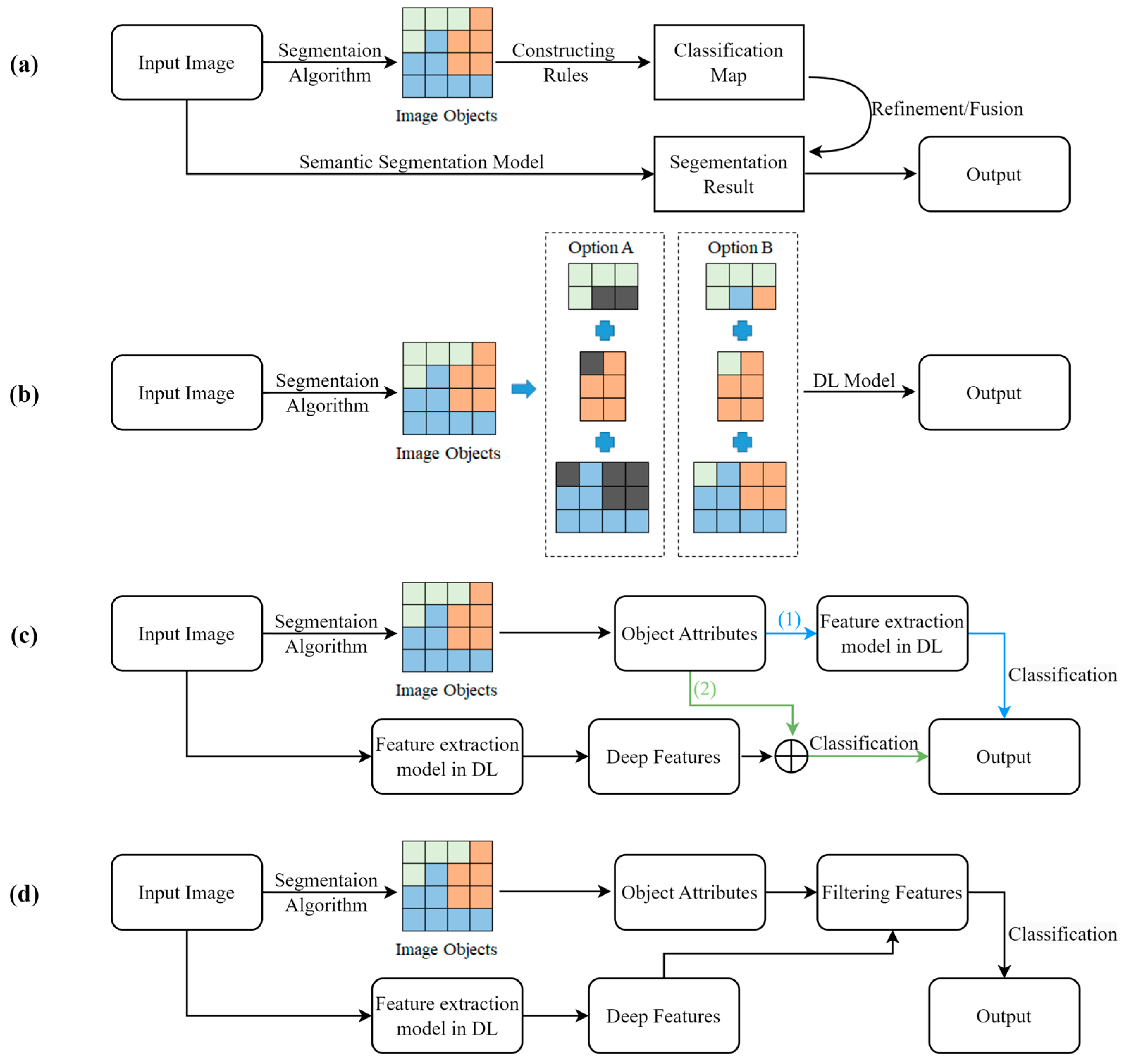
2.2. Deep Learning Framework Coupled with GEOBIA
2.3. Attention Mechanism
3. Method
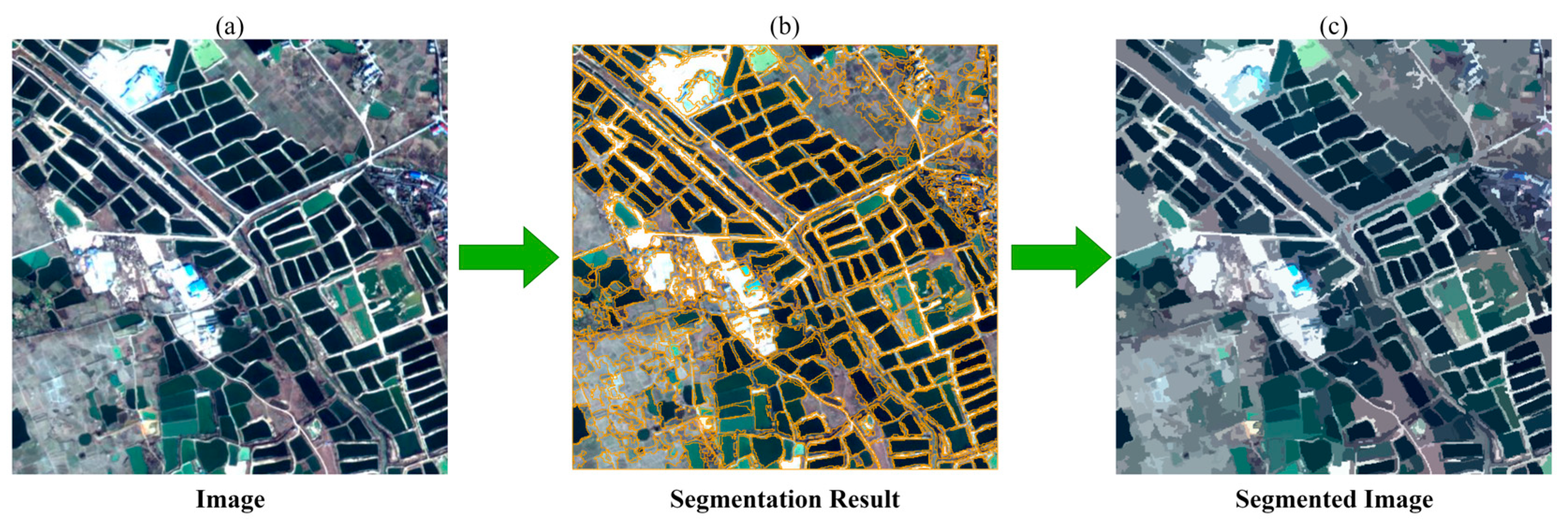
3.1. Multi-Scale Segmentation Optimization Algorithm—EIODA
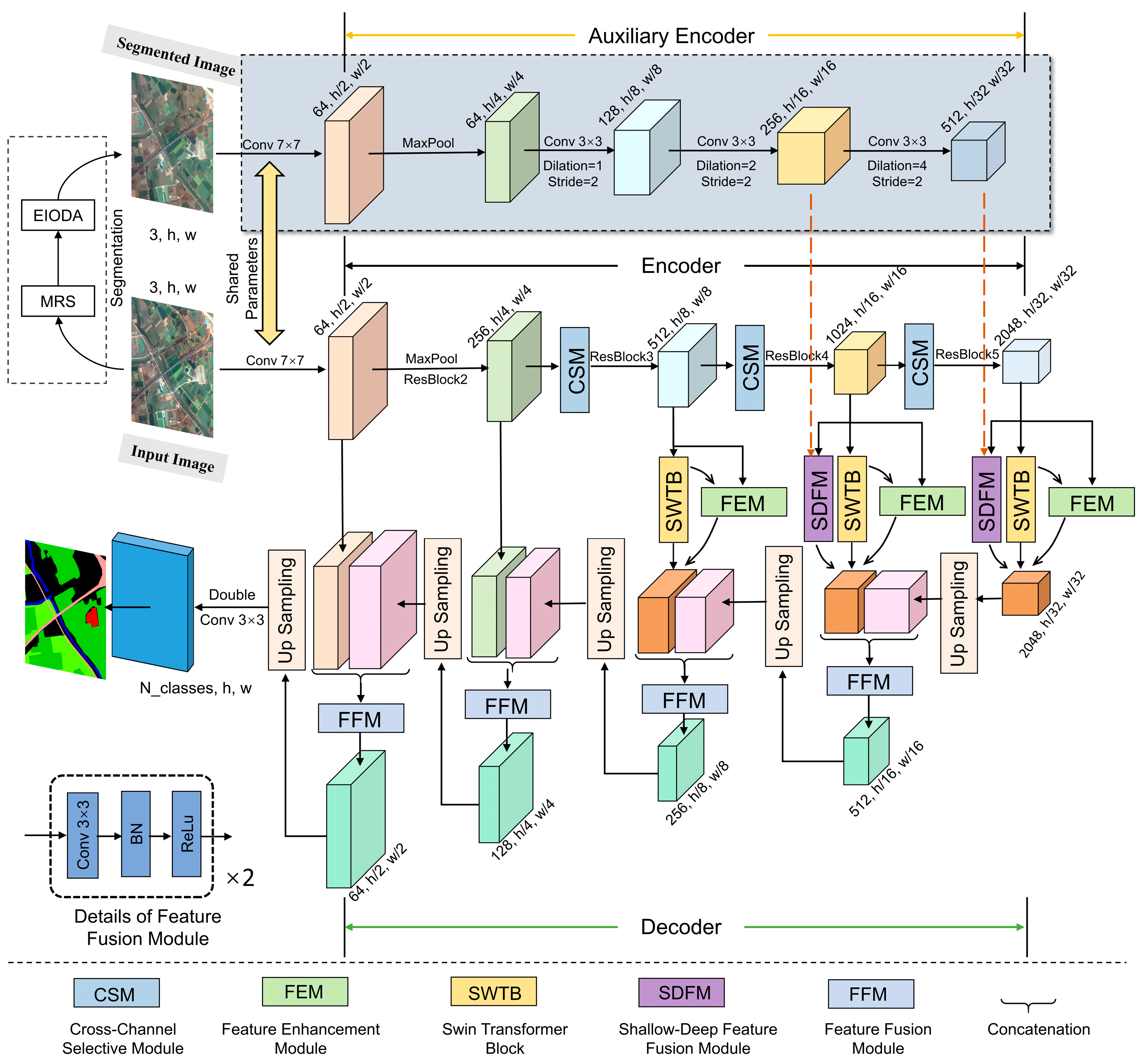
3.2. Overall Network Structure
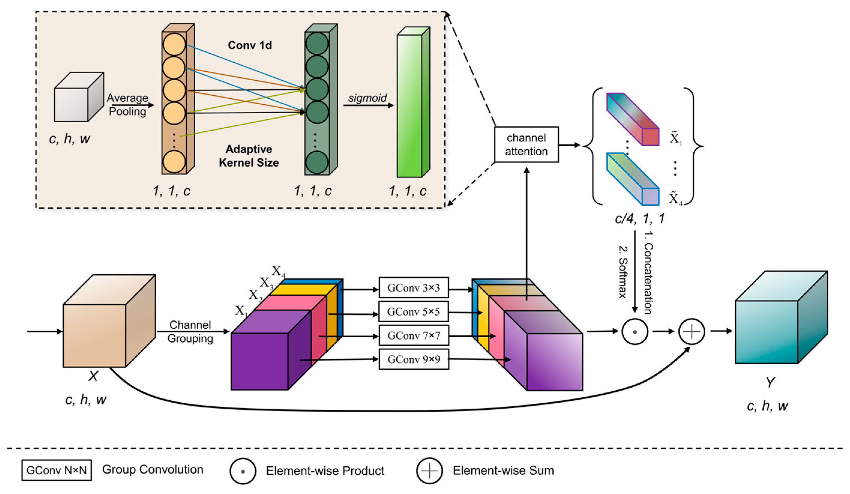
3.3. Cross-Channel Selective Module
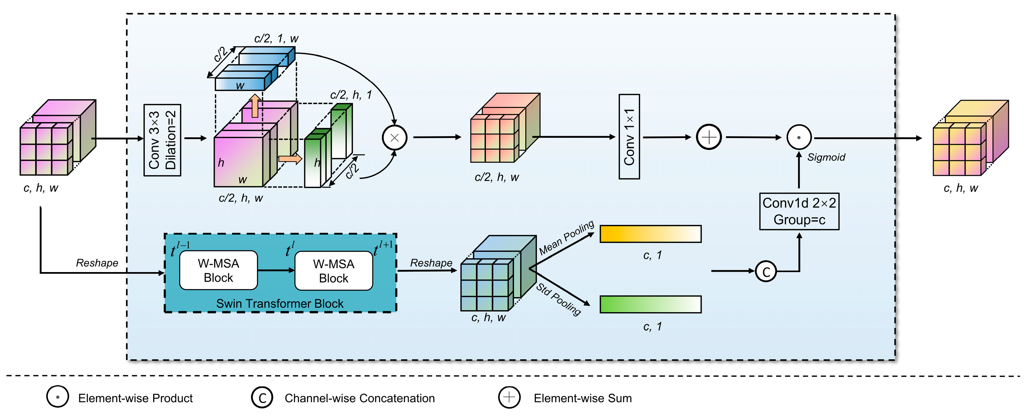
3.4. Feature Enhancement Module
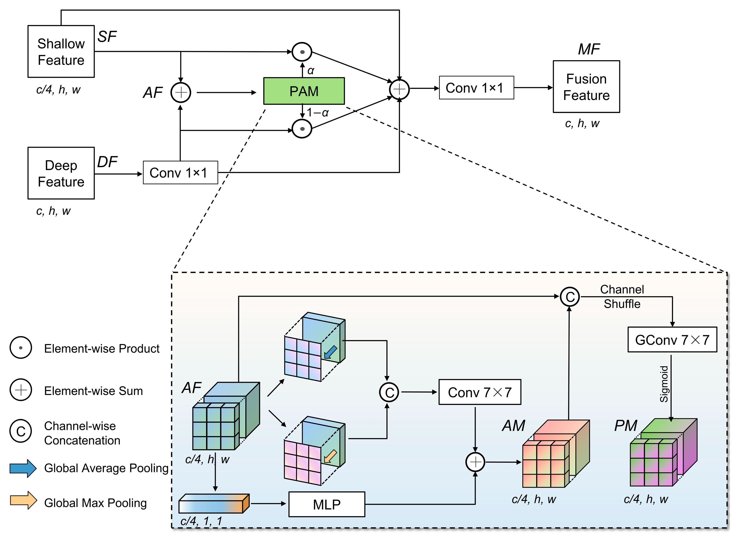
3.5. Shallow–Deep Feature Fusion Module
4. Results
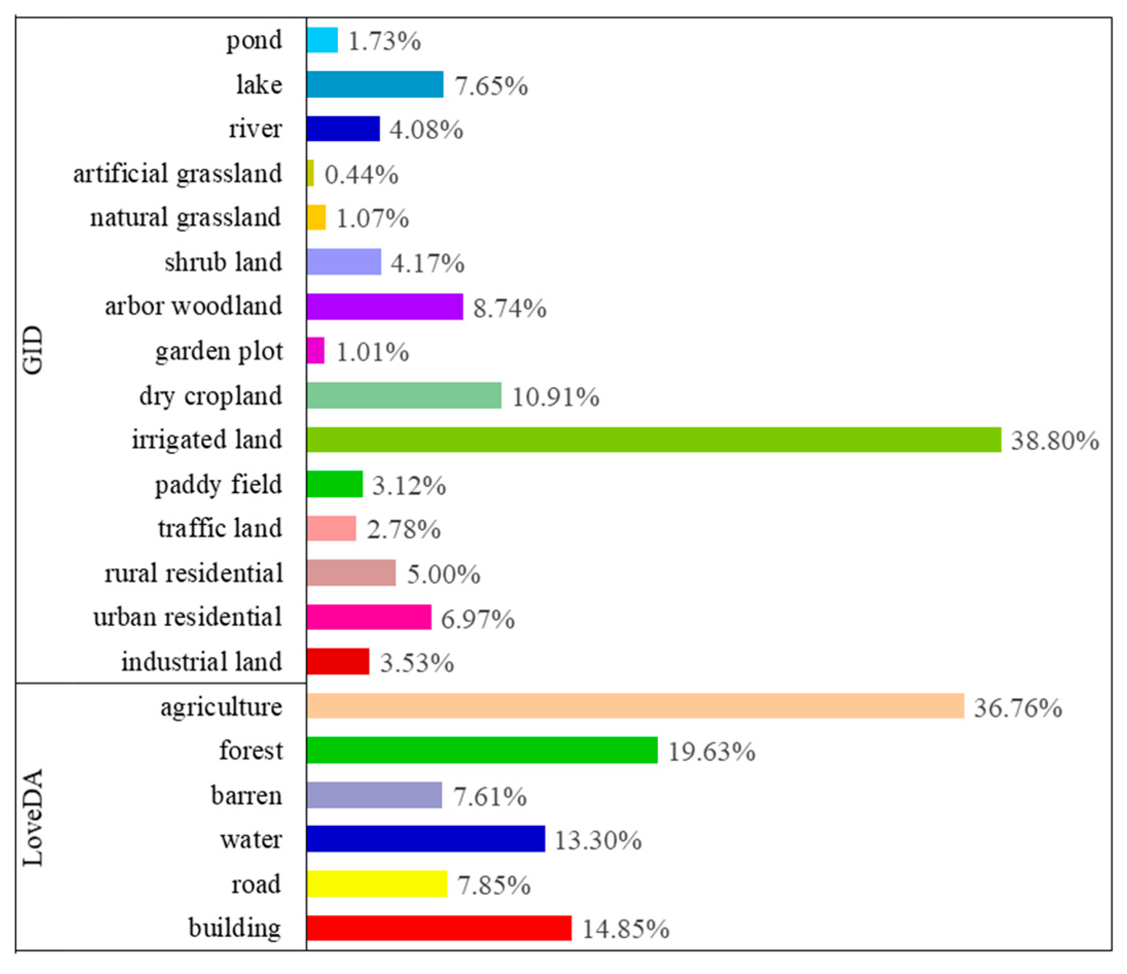
4.1. Datasets
4.1.1. GID
4.1.2. LoveDA Dataset
4.2. Implementation Details
4.2.1. Experimental Settings
4.2.2. Loss Function
4.2.3. Evaluation Metrics
4.3. Ablation Study
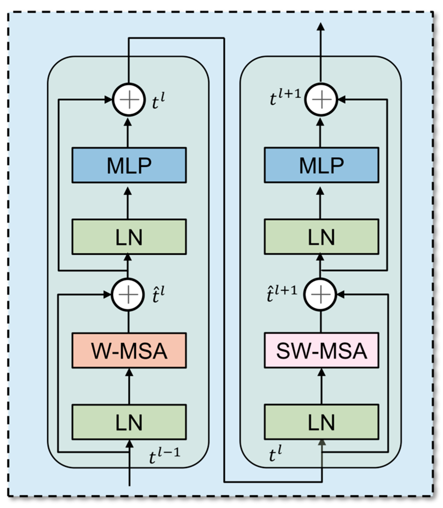
4.3.1. Effect of Integrating SWTB (Baseline)
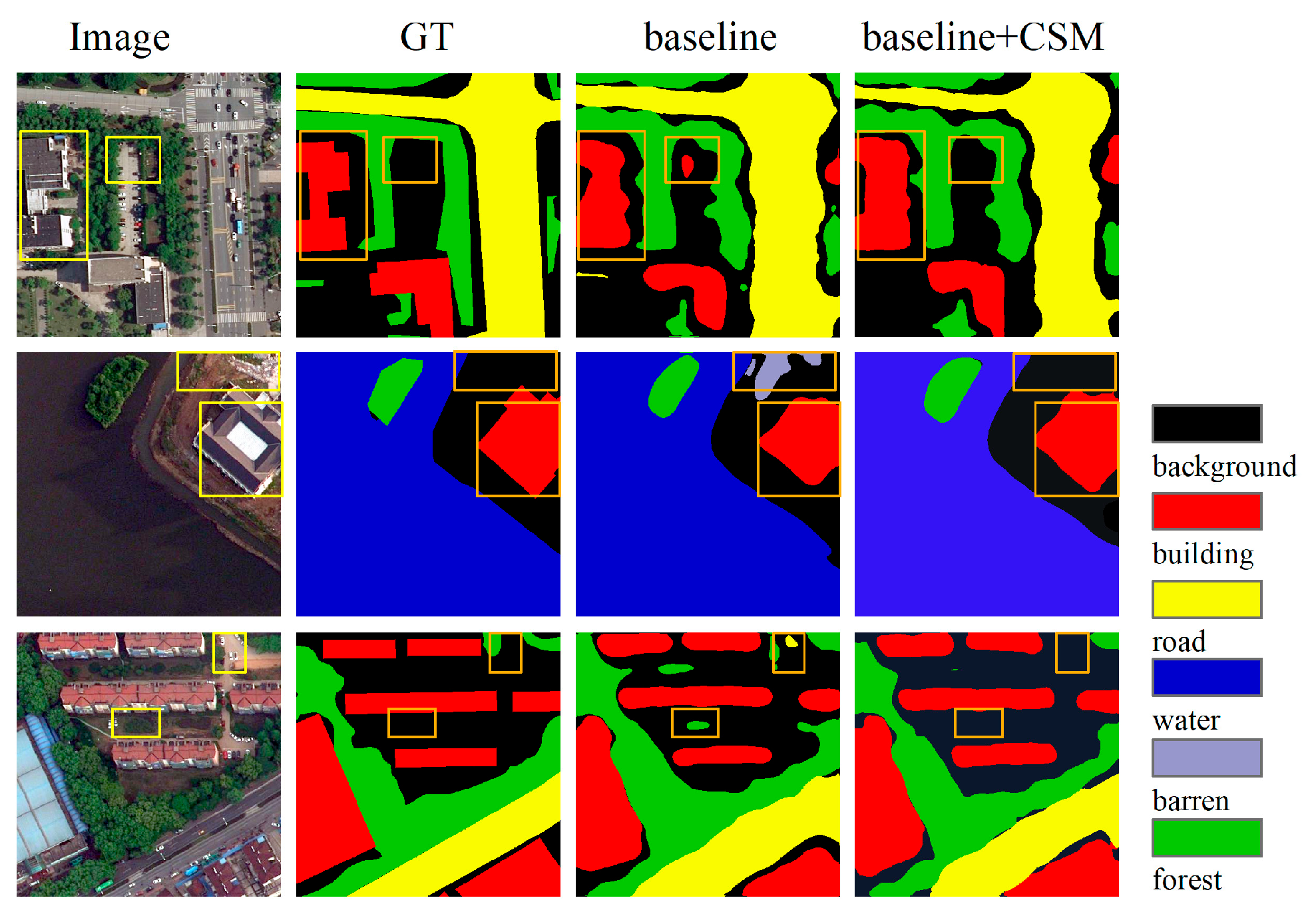
4.3.2. Effect of Cross-Channel Selective Module
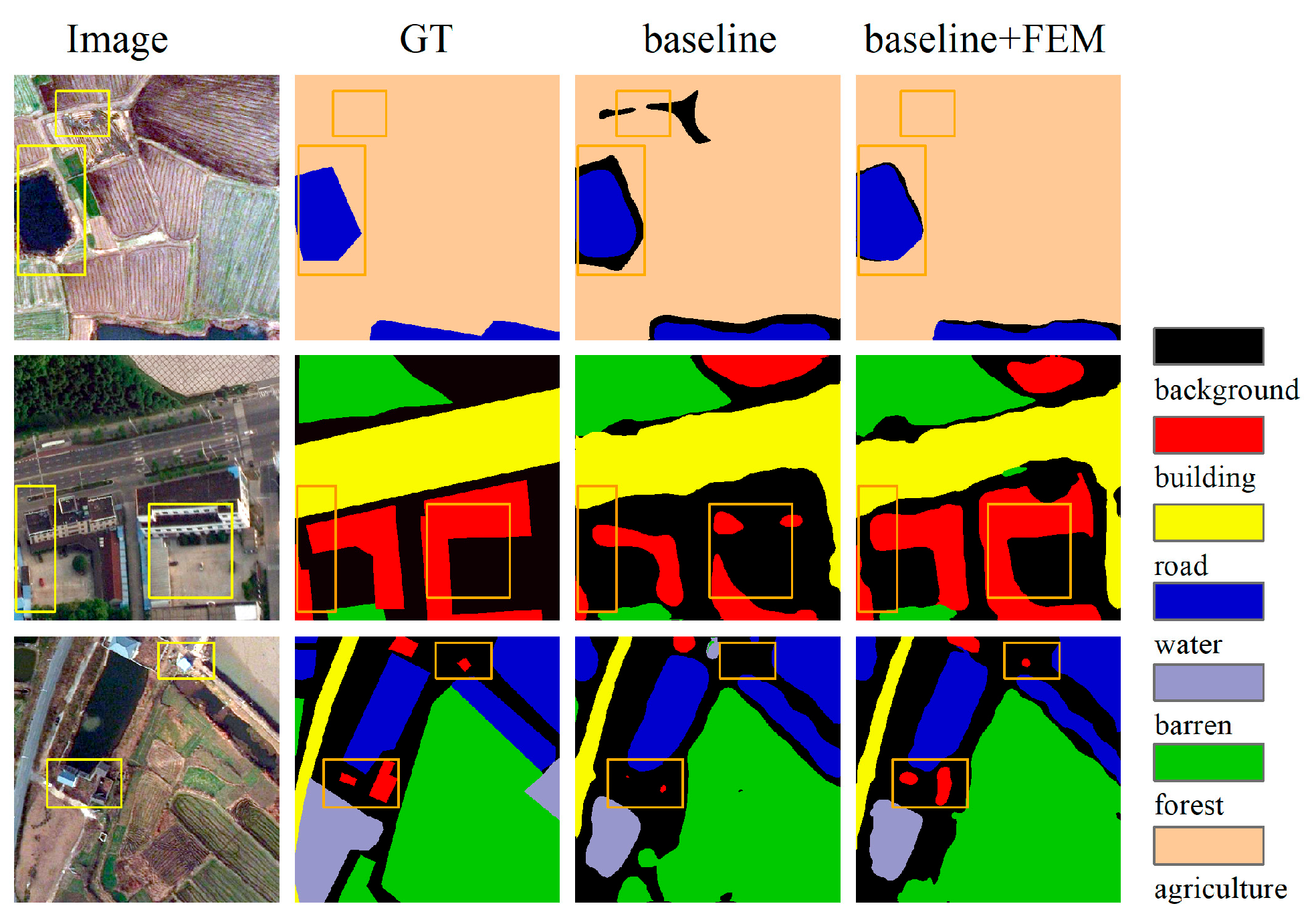
4.3.3. Effect of Feature Enhancement Module
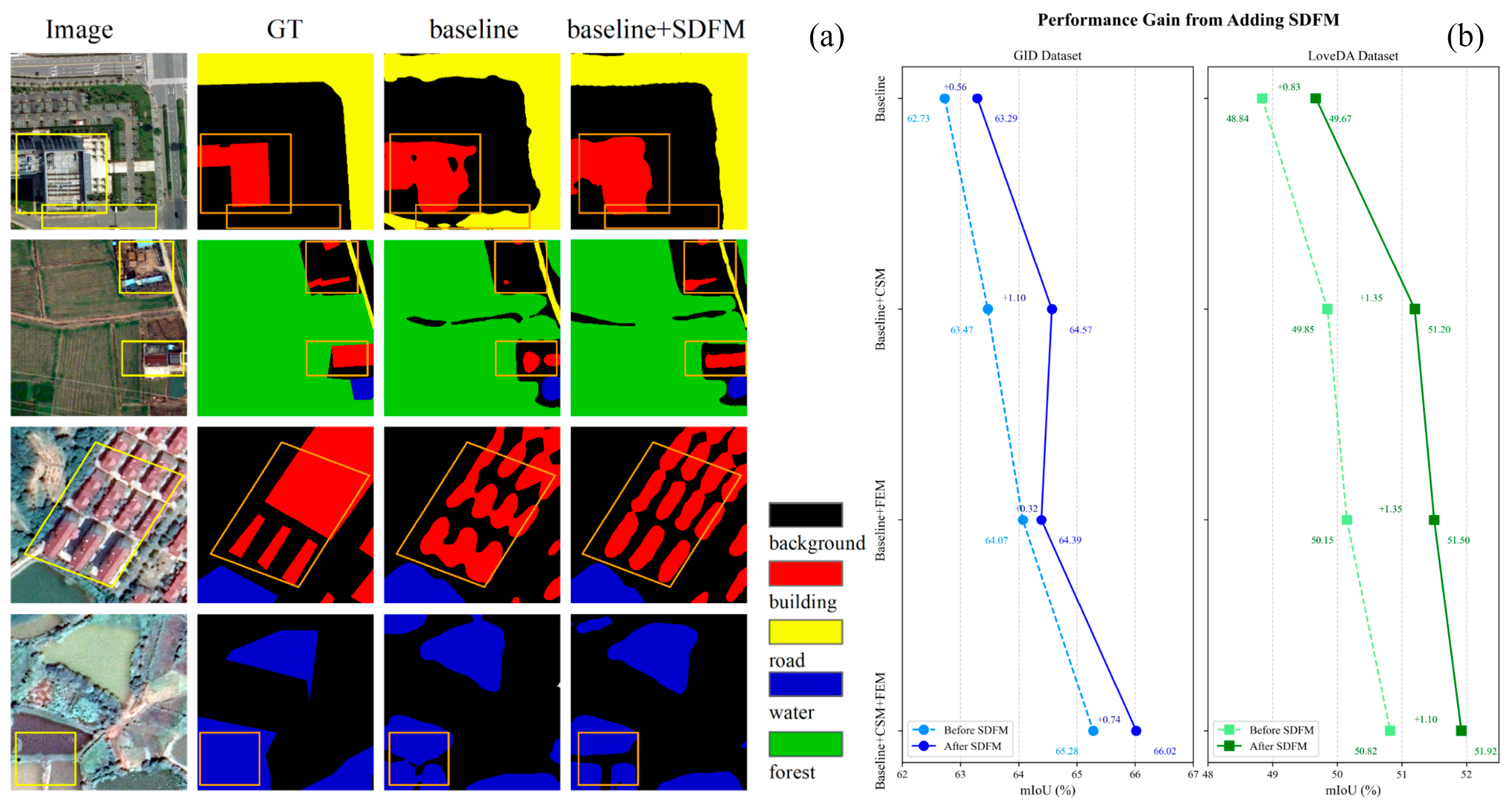
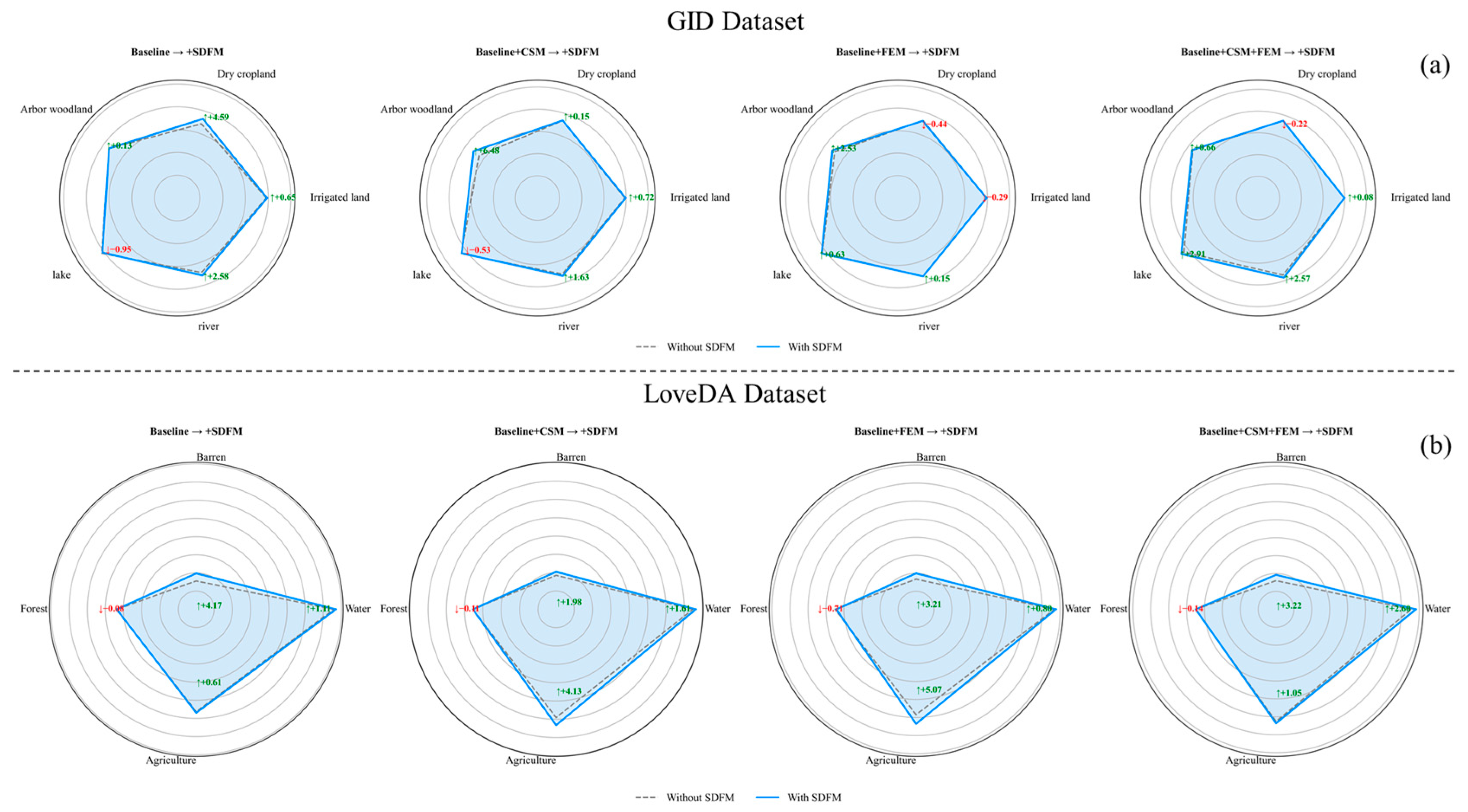
4.3.4. Effect of Shallow–Deep Feature Fusion Module
4.3.5. Joint Effects of Different Modules

| Model Name | Module | GID | LoveDA | |||||||||||
|---|---|---|---|---|---|---|---|---|---|---|---|---|---|---|
| CCM | FEM | SDFM | mIoU (%) | mPA (%) | OA (%) | IoU per Category (%) | mIoU (%) | |||||||
| Background | Building | Road | Water | Barren | Forest | Agriculture | ||||||||
| Baseline | 62.73 | 74.89 | 82.60 | 43.59 | 51.67 | 55.06 | 75.80 | 15.62 | 43.84 | 56.27 | 48.84 | |||
| Baseline + CSM | ✓ | 63.47 | 74.01 | 82.99 | 44.14 | 52.87 | 54.06 | 74.67 | 18.55 | 45.57 | 59.06 | 49.85 | ||
| Baseline + FEM | ✓ | 64.07 | 74.75 | 83.44 | 43.30 | 55.64 | 55.08 | 76.81 | 16.78 | 45.01 | 58.44 | 50.15 | ||
| Baseline + SDFM | ✓ | 63.29 | 75.43 | 83.13 | 42.79 | 53.52 | 54.04 | 76.91 | 19.79 | 43.76 | 56.88 | 49.67 | ||
| Baseline + CSM + FEM | ✓ | ✓ | 65.28 | 76.49 | 83.99 | 44.36 | 56.55 | 55.64 | 75.53 | 16.06 | 45.02 | 62.55 | 50.82 | |
| Baseline + CSM + SDFM | ✓ | ✓ | 64.57 | 75.69 | 83.63 | 43.26 | 55.46 | 54.23 | 76.28 | 20.53 | 45.46 | 63.19 | 51.20 | |
| Baseline + FEM + SDFM | ✓ | ✓ | 64.39 | 75.37 | 83.52 | 44.34 | 55.04 | 55.73 | 77.61 | 19.99 | 44.30 | 63.51 | 51.50 | |
| Baseline + CSM + FEM + SDFM | ✓ | ✓ | ✓ | 66.02 | 77.78 | 84.07 | 45.20 | 55.63 | 56.75 | 78.13 | 19.28 | 44.88 | 63.60 | 51.92 |
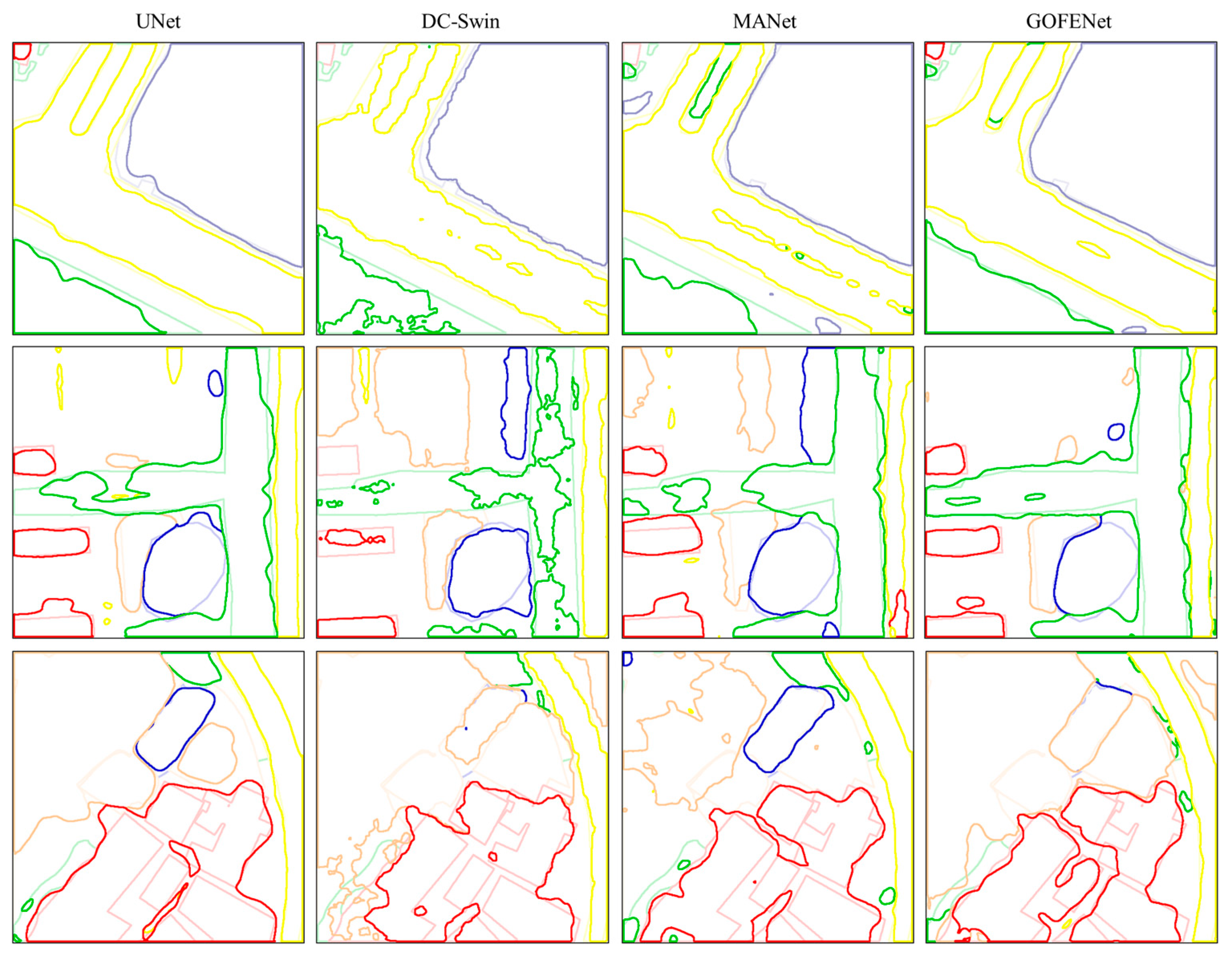
4.4. Performance Evaluation and Comparisons with Other Models
| Method | Backbone | IoU per Category (%) | mIoU (%) | mPA (%) | OA (%) | |||||||||||||||
|---|---|---|---|---|---|---|---|---|---|---|---|---|---|---|---|---|---|---|---|---|
| BG | INL | UR | RU | TL | PF | IL | DC | GP | AW | SL | NG | AG | RI | LA | PD | |||||
| UNet [19] | ResNet50 | 64.07 | 57.72 | 68.68 | 59.62 | 51.60 | 72.48 | 77.86 | 67.43 | 30.53 | 72.55 | 68.73 | 38.51 | 32.53 | 67.56 | 81.66 | 44.22 | 59.73 | 75.23 | 80.98 |
| PSPNet [24] | ResNet50 | 64.73 | 58.35 | 68.26 | 59.43 | 43.60 | 72.03 | 76.42 | 69.74 | 32.43 | 73.34 | 68.19 | 43.96 | 35.65 | 71.49 | 85.67 | 47.06 | 60.65 | 71.95 | 81.25 |
| SegNet [72] | ResNet50 | 62.39 | 55.41 | 67.00 | 55.80 | 43.01 | 66.36 | 75.05 | 65.22 | 31.85 | 71.07 | 67.16 | 45.85 | 29.24 | 65.73 | 75.81 | 45.98 | 57.68 | 71.53 | 79.32 |
| DeeplabV3+ [23] | ResNet50 | 65.15 | 57.69 | 67.12 | 58.73 | 48.06 | 71.42 | 75.88 | 70.07 | 34.43 | 72.45 | 69.41 | 45.80 | 32.79 | 68.12 | 80.52 | 48.20 | 60.37 | 74.08 | 80.91 |
| DANet [25] | ResNet50 | 65.82 | 58.25 | 67.93 | 59.51 | 48.09 | 71.99 | 75.49 | 71.10 | 29.30 | 72.45 | 67.79 | 42.71 | 37.86 | 73.22 | 85.44 | 48.93 | 60.99 | 74.29 | 81.32 |
| SegFormer [36] | MIT-B1 | 66.91 | 58.35 | 68.54 | 59.72 | 47.48 | 72.30 | 77.53 | 71.85 | 30.62 | 74.00 | 69.40 | 50.05 | 32.74 | 72.71 | 85.43 | 50.23 | 61.74 | 73.70 | 82.23 |
| DC-Swin [39] | Swin-Tiny | 65.91 | 57.34 | 67.38 | 59.41 | 46.35 | 69.29 | 76.36 | 70.29 | 32.51 | 73.10 | 68.08 | 48.01 | 33.06 | 72.38 | 86.93 | 50.94 | 61.08 | 72.98 | 81.51 |
| MANet [71] | ResNet50 | 68.77 | 60.81 | 70.23 | 62.00 | 54.28 | 73.13 | 78.84 | 73.75 | 37.82 | 75.60 | 72.21 | 51.00 | 35.79 | 77.56 | 88.28 | 54.41 | 64.69 | 76.23 | 83.59 |
| UNetFormer [44] | ResNet18 | 67.82 | 61.20 | 70.22 | 61.32 | 53.85 | 72.56 | 77.56 | 71.73 | 36.47 | 73.59 | 70.06 | 52.86 | 36.46 | 75.19 | 87.28 | 52.54 | 63.79 | 75.74 | 82.80 |
| LMA-Swin [41] | Swin-Small | 68.50 | 59.10 | 70.61 | 62.63 | 55.46 | 70.83 | 77.68 | 73.32 | 37.19 | 74.76 | 70.93 | 45.99 | 37.62 | 76.84 | 88.37 | 50.61 | 63.78 | 74.79 | 83.12 |
| GOFENet (ours) | ResNet50 | 69.24 | 61.77 | 71.33 | 63.68 | 55.90 | 74.79 | 79.66 | 74.82 | 40.38 | 75.24 | 72.89 | 55.25 | 40.43 | 77.06 | 87.55 | 56.35 | 66.02 | 77.78 | 84.07 |
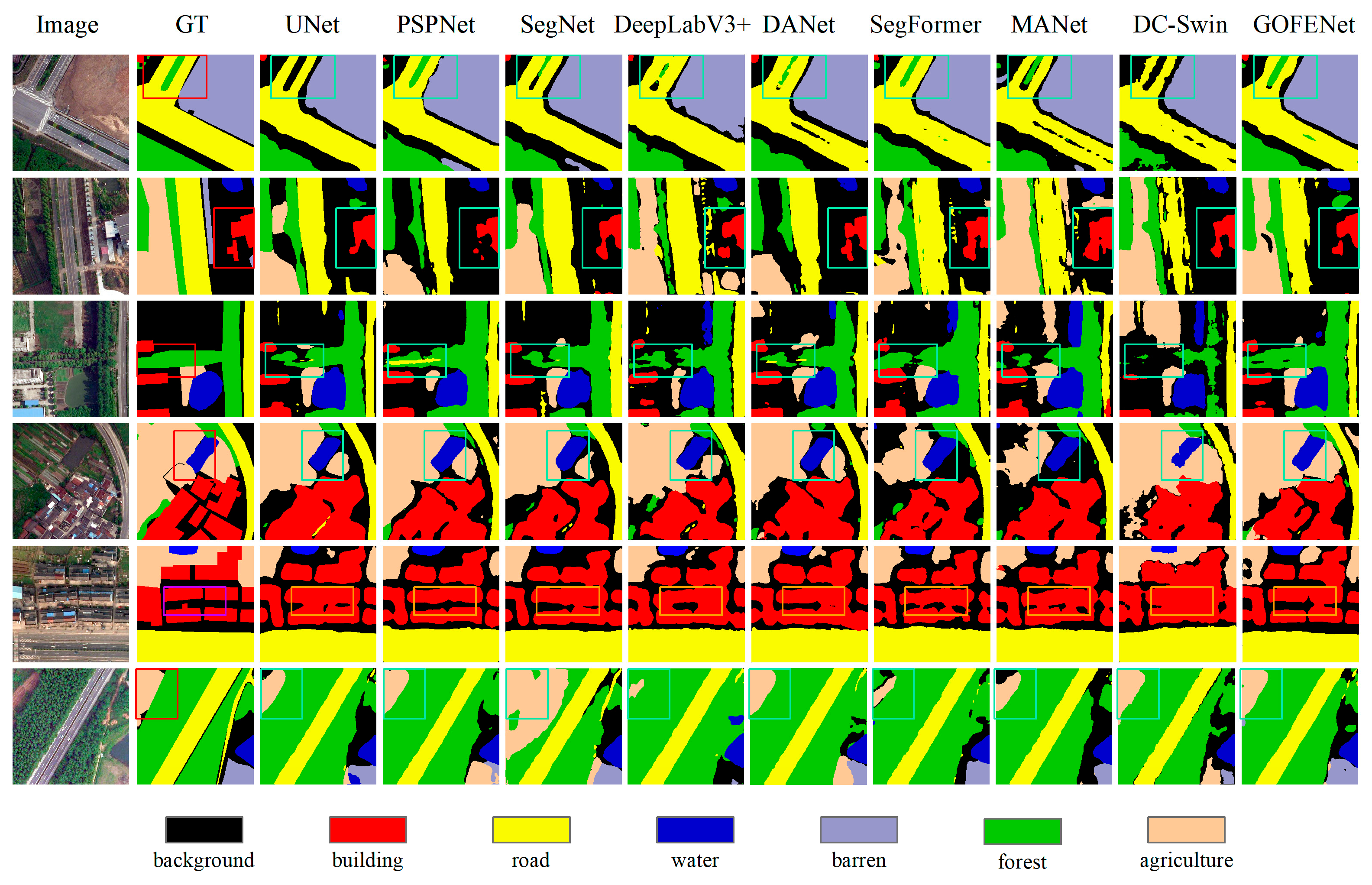
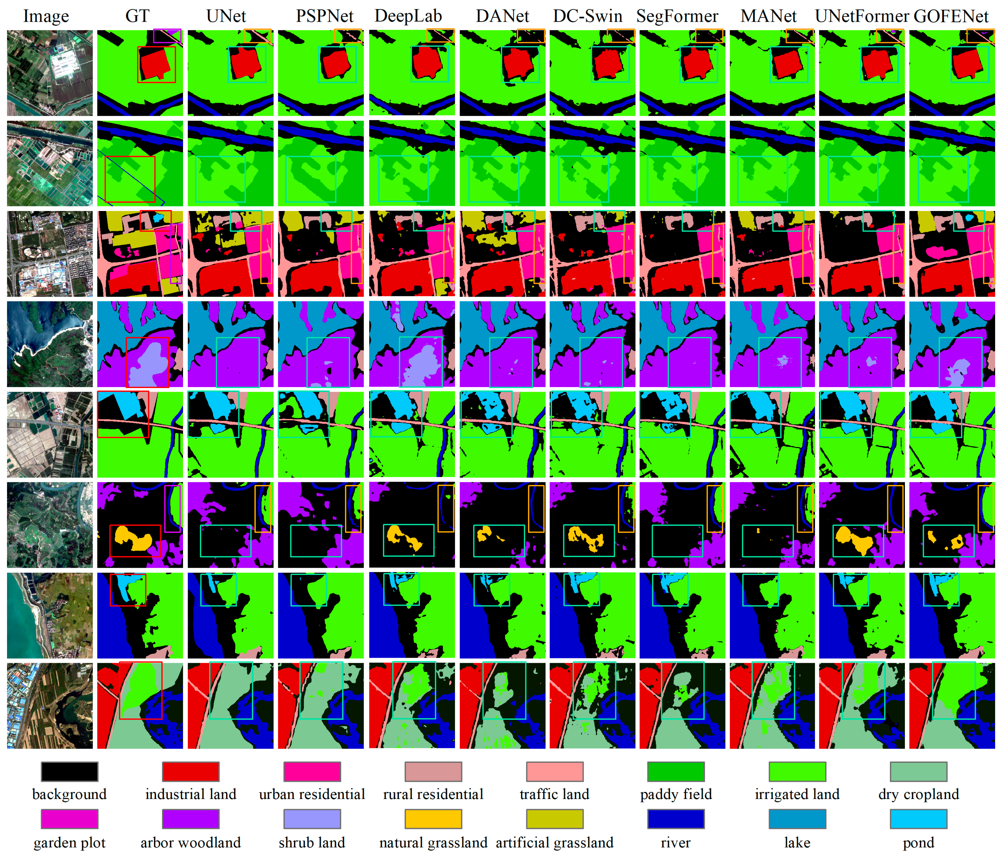
4.4.1. Results on GID
4.4.2. Results on the LoveDA Dataset
| Method | Backbone | IoU per Category (%) | mIoU (%) | ||||||
|---|---|---|---|---|---|---|---|---|---|
| Background | Building | Road | Water | Barren | Forest | Agriculture | |||
| UNet [19] | ResNet50 | 43.1 | 52.7 | 52.8 | 73.1 | 10.3 | 43.1 | 59.9 | 47.8 |
| PSPNet [24] | ResNet50 | 44.4 | 52.1 | 53.5 | 76.5 | 9.7 | 44.1 | 57.9 | 48.3 |
| SegNet [72] | ResNet50 | 43.4 | 53.0 | 52.9 | 76.0 | 12.7 | 44.0 | 54.8 | 48.1 |
| DeeplabV3+ [23] | ResNet50 | 43.0 | 50.9 | 52.0 | 74.4 | 10.4 | 44.2 | 58.5 | 47.6 |
| Segmenter [35] | Vit-Tiny | 38.0 | 50.7 | 48.7 | 77.4 | 13.3 | 43.5 | 58.2 | 47.1 |
| BANet [40] | ResT-Lite | 43.7 | 51.5 | 51.1 | 76.9 | 16.6 | 44.9 | 62.5 | 49.6 |
| DANet [25] | ResNet50 | 44.8 | 55.5 | 53.0 | 75.5 | 17.6 | 45.1 | 60.1 | 50.2 |
| LANet [74] | ResNet50 | 40.0 | 50.6 | 51.1 | 78.0 | 13.0 | 43.2 | 56.9 | 47.6 |
| SegFormer [36] | MIT-B1 | 43.0 | 52.2 | 53.2 | 68.6 | 10.3 | 45.4 | 53.1 | 46.5 |
| FactSeg [73] | ResNet50 | 42.6 | 53.6 | 52.8 | 76.9 | 16.2 | 42.9 | 57.5 | 48.9 |
| MANet [71] | ResNet50 | 38.7 | 51.7 | 42.6 | 72.0 | 15.3 | 42.1 | 57.7 | 45.7 |
| HRNet [75] | W32 | 44.6 | 55.3 | 57.4 | 74.0 | 11.1 | 45.3 | 60.9 | 49.8 |
| DC-Swin [39] | Swin-Tiny | 41.3 | 54.5 | 56.2 | 78.1 | 14.5 | 47.2 | 62.4 | 50.6 |
| TransUNet [78] | ViT-R50 | 43.0 | 56.1 | 53.7 | 78.0 | 9.3 | 44.9 | 56.9 | 48.9 |
| SwinUperNet [30] | Swin-Tiny | 43.3 | 54.3 | 54.3 | 78.7 | 14.9 | 45.3 | 59.6 | 50.0 |
| C-PNet [76] | - | 44.0 | 55.2 | 55.3 | 78.8 | 16.0 | 46.4 | 58.0 | 51.8 |
| Mask2Former [77] | Swin-Small | 44.8 | 56.8 | 55.5 | 78.6 | 17.8 | 46.3 | 60.0 | 51.5 |
| ESDINet [79] | ResNet18 | 41.6 | 53.8 | 54.8 | 78.7 | 19.5 | 44.2 | 58.0 | 50.1 |
| GOFENet (ours) | ResNet50 | 45.2 | 55.6 | 56.7 | 78.1 | 19.3 | 44.9 | 63.6 | 51.9 |
5. Discussion
5.1. Design of Auxiliary Branch
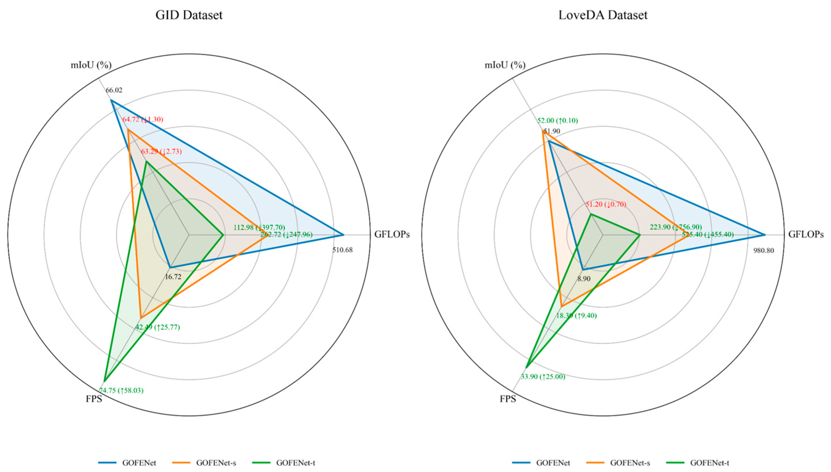
5.2. Model Efficiency Analysis
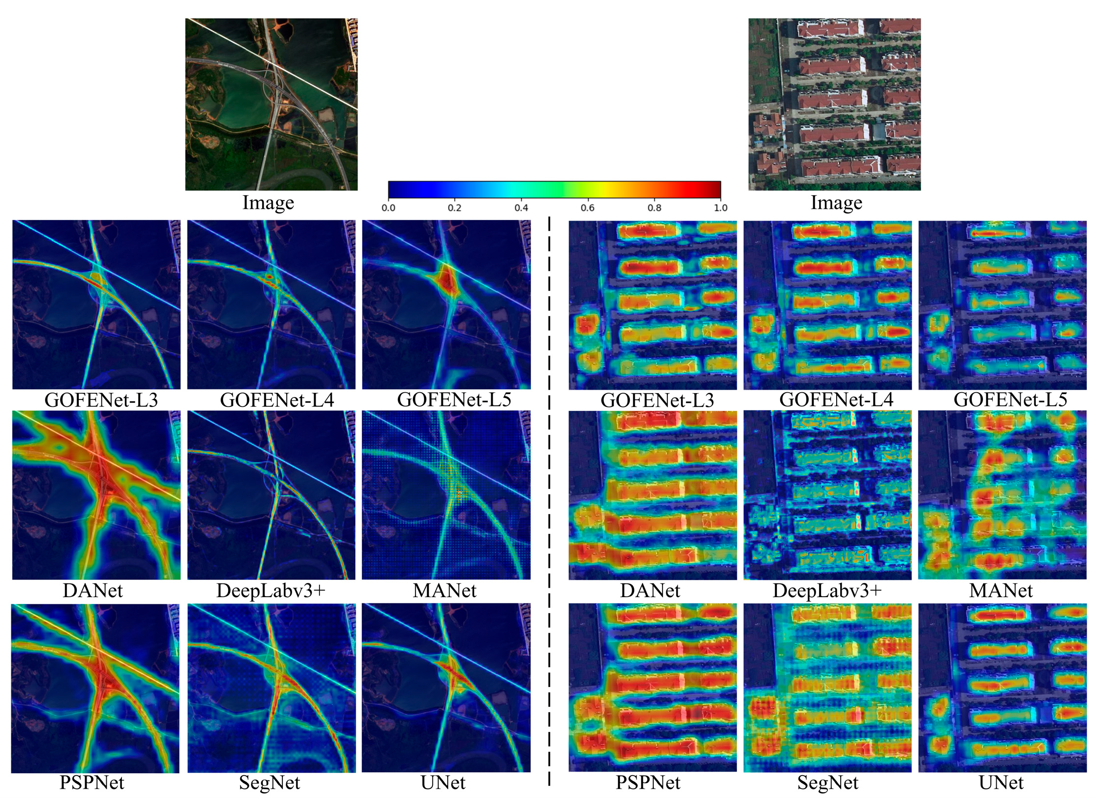
5.3. Grad-CAM Visualization
5.4. Advantages and Limitations of Embedded Object Features
6. Conclusions
Author Contributions
Funding
Data Availability Statement
Conflicts of Interest
References
- Lei, P.; Yi, J.; Li, S.; Li, Y.; Lin, H. Agricultural Surface Water Extraction in Environmental Remote Sensing: A Novel Semantic Segmentation Model Emphasizing Contextual Information Enhancement and Foreground Detail Attention. Neurocomputing 2025, 617, 129110. [Google Scholar] [CrossRef]
- Liu, Y.; Zhong, Y.; Shi, S.; Zhang, L. Scale-Aware Deep Reinforcement Learning for High Resolution Remote Sensing Imagery Classification. ISPRS J. Photogramm. Remote Sens. 2024, 209, 296–311. [Google Scholar] [CrossRef]
- Wang, Y.; Sun, Y.; Cao, X.; Wang, Y.; Zhang, W.; Cheng, X. A Review of Regional and Global Scale Land Use/Land Cover (LULC) Mapping Products Generated from Satellite Remote Sensing. ISPRS J. Photogramm. Remote Sens. 2023, 206, 311–334. [Google Scholar] [CrossRef]
- Zhu, Q.; Guo, X.; Deng, W.; Shi, S.; Guan, Q.; Zhong, Y.; Zhang, L.; Li, D. Land-Use/Land-Cover Change Detection Based on a Siamese Global Learning Framework for High Spatial Resolution Remote Sensing Imagery. ISPRS J. Photogramm. Remote Sens. 2022, 184, 63–78. [Google Scholar] [CrossRef]
- Zhang, T.; Huang, X. Monitoring of Urban Impervious Surfaces Using Time Series of High-Resolution Remote Sensing Images in Rapidly Urbanized Areas: A Case Study of Shenzhen. IEEE J. Sel. Top. Appl. Earth Obs. Remote Sens. 2018, 11, 2692–2708. [Google Scholar] [CrossRef]
- Chen, B.; Qiu, F.; Wu, B.; Du, H. Image Segmentation Based on Constrained Spectral Variance Difference and Edge Penalty. Remote Sens. 2015, 7, 5980–6004. [Google Scholar] [CrossRef]
- Zhou, Y.; Feng, L.; Chen, Y.; Li, J. Object-Based Land Cover Mapping Using Adaptive Scale Segmentation From ZY-3 Satellite Images. In Proceedings of the 2017 IEEE International Geoscience and Remote Sensing Symposium (IGARSS), Fort Worth, TX, USA, 23–28 July 2017; IEEE: New York, NY, USA; pp. 63–66. [Google Scholar]
- Thenkabail, P.S. Remotely Sensed Data Characterization, Classification, and Accuracies; CRC Press: Boca Raton, FL, USA, 2015. [Google Scholar]
- Derivaux, S.; Lefevre, S.; Wemmert, C.; Korczak, J. Watershed Segmentation of Remotely Sensed Images Based on a Supervised Fuzzy Pixel Classification. In Proceedings of the 2006 IEEE International Symposium on Geoscience and Remote Sensing, Denver, CO, USA, 31 July–4 August 2006; IEEE: New York, NY, USA, 2006; pp. 3712–3715. [Google Scholar]
- Baatz, M.; Schäpe, A. Multiresolution Segmentation: An Optimization Approach for High Quality Multi-Scale Image Segmentation. In Angewandte Geographische Informationsverarbeitung XII; Wichmann Verlag: Karlsruhe, Germany, 2000; pp. 12–23. [Google Scholar]
- Tzotsos, A.; Argialas, D. MSEG: A Generic Region-Based Multi-Scale Image Segmentation Algorithm for Remote Sensing Imagery. In Proceedings of the ASPRS 2006 Annual Conference, Reno, NV, USA, 1–5 May 2006. [Google Scholar]
- Yang, J.; He, Y.; Caspersen, J. Region Merging Using Local Spectral Angle Thresholds: A More Accurate Method for Hybrid Segmentation of Remote Sensing Images. Remote Sens. Environ. 2017, 190, 137–148. [Google Scholar] [CrossRef]
- Blaschke, T.; Hay, G.J.; Kelly, M.; Lang, S.; Hofmann, P.; Addink, E.; Feitosa, R.Q.; Van der Meer, F.; Van der Werff, H.; Van Coillie, F.; et al. Geographic Object-Based Image Analysis–Towards a New Paradigm. ISPRS J. Photogramm. Remote Sens. 2014, 87, 180–191. [Google Scholar] [CrossRef]
- Hu, Y.; Chen, J.; Pan, D.; Hao, Z. Edge-Guided Image Object Detection in Multiscale Segmentation for High-Resolution Remotely Sensed Imagery. IEEE Trans. Geosci. Remote Sens. 2016, 54, 4702–4711. [Google Scholar] [CrossRef]
- Shen, Y.; Chen, J.; Xiao, L.; Pan, D. Optimizing Multiscale Segmentation with Local Spectral Heterogeneity Measure for High Resolution Remote Sensing Images. ISPRS J. Photogramm. Remote Sens. 2019, 157, 13–25. [Google Scholar] [CrossRef]
- He, T.; Chen, J.; Kang, L.; Zhu, Q. Evaluation of Global-Scale and Local-Scale Optimized Segmentation Algorithms in GEOBIA With SAM on Land Use and Land Cover. IEEE J. Sel. Top. Appl. Earth Obs. Remote Sens. 2024, 17, 6721–6738. [Google Scholar] [CrossRef]
- Long, J.; Shelhamer, E.; Darrell, T. Fully Convolutional Networks for Semantic Segmentation. In Proceedings of the IEEE Conference on Computer Vision and Pattern Recognition, Boston, MA, USA, 7–12 June 2015; pp. 3431–3440. [Google Scholar]
- He, K.; Zhang, X.; Ren, S.; Sun, J. Deep Residual Learning for Image Recognition. In Proceedings of the IEEE Conference on Computer Vision and Pattern Recognition, Las Vegas, NV, USA, 27–30 June 2016; pp. 770–778. [Google Scholar]
- Ronneberger, O.; Fischer, P.; Brox, T. U-net: Convolutional Networks for Biomedical Image Segmentation. In Proceedings of the Medical Image Computing and Computer-Assisted Intervention–MICCAI 2015: 18th International Conference, Munich, Germany, 5–9 October 2015; Springer: Cham, Switzerland, 2015. proceedings, part III 18. pp. 234–241. [Google Scholar]
- Xiang, X.; Gong, W.; Li, S.; Chen, J.; Ren, T. TCNet: Multiscale Fusion of Transformer and CNN for Semantic Segmentation of Remote Sensing Images. IEEE J. Sel. Top. Appl. Earth Obs. Remote Sens. 2024, 17, 3123–3136. [Google Scholar] [CrossRef]
- Liu, B.; Li, B.; Sreeram, V.; Li, S. MBT-UNet: Multi-Branch Transform Combined with UNet for Semantic Segmentation of Remote Sensing Images. Remote Sens. 2024, 16, 2776. [Google Scholar] [CrossRef]
- Ren, X.; Deng, Z.; Ye, J.; He, J.; Yang, D. FCN+: Global Receptive Convolution Makes Fcn Great Again. Neurocomputing 2025, 631, 129655. [Google Scholar] [CrossRef]
- Chen, L.-C.; Zhu, Y.; Papandreou, G.; Schroff, F.; Adam, H. Encoder-Decoder with Atrous Separable Convolution for Semantic Image Segmentation. In Proceedings of the European Conference on Computer Vision (ECCV), Munich, Germany, 8–14 September 2018; pp. 801–818. [Google Scholar]
- Zhao, H.; Shi, J.; Qi, X.; Wang, X.; Jia, J. Pyramid Scene Parsing Network. In Proceedings of the IEEE Conference on Computer Vision and Pattern Recognition, Honolulu, HI, USA, 21–26 July 2017; pp. 2881–2890. [Google Scholar]
- Fu, J.; Liu, J.; Tian, H.; Li, Y.; Bao, Y.; Fang, Z.; Lu, H. Dual Attention Network for Scene Segmentation. In Proceedings of the IEEE/CVF Conference on Computer Vision and Pattern Recognition, Long Beach, CA, USA, 15–20 June 2019; pp. 3146–3154. [Google Scholar]
- Woo, S.; Park, J.; Lee, J.-Y.; Kweon, I.S. Cbam: Convolutional Block Attention Module. In Proceedings of the European Conference on Computer Vision (ECCV), Munich, Germany, 8–14 September 2018; pp. 3–19. [Google Scholar]
- Khan, S.; Naseer, M.; Hayat, M.; Zamir, S.W.; Khan, F.S.; Shah, M. Transformers in Vision: A Survey. ACM Comput. Surv. 2022, 54, 1–41. [Google Scholar] [CrossRef]
- Alexey, D. An Image is Worth 16x16 Words: Transformers for Image Recognition at scale. arXiv 2020, arXiv:2010.11929. [Google Scholar]
- Zheng, S.; Lu, J.; Zhao, H.; Zhu, X.; Luo, Z.; Wang, Y.; Fu, Y.; Feng, J.; Xiang, T.; Torr, P.H.; et al. Rethinking Semantic Segmentation from a Sequence-to-Sequence Perspective with Transformers. In Proceedings of the IEEE/CVF Conference on Computer Vision and Pattern Recognition, Nashville, TN, USA, 20–25 June 2021; pp. 6881–6890. [Google Scholar]
- Liu, Z.; Lin, Y.; Cao, Y.; Hu, H.; Wei, Y.; Zhang, Z.; Lin, S.; Guo, B. Swin Transformer: Hierarchical Vision Transformer Using Shifted Windows. In Proceedings of the IEEE/CVF International Conference on Computer Vision, Montreal, QC, Canada, 10–17 October 2021; pp. 10012–10022. [Google Scholar]
- Bai, Q.; Luo, X.; Wang, Y.; Wei, T. DHRNet: A Dual-Branch Hybrid Reinforcement Network for Semantic Segmentation of Remote Sensing Images. IEEE J. Sel. Top. Appl. Earth Obs. Remote Sens. 2024, 17, 4176–4193. [Google Scholar] [CrossRef]
- Gao, Y.; Luo, X.; Gao, X.; Yan, W.; Pan, X.; Fu, X. Semantic Segmentation of Remote Sensing Images Based on Multiscale Features and Global Information Modeling. Expert Syst. Appl. 2024, 249, 123616. [Google Scholar] [CrossRef]
- Yang, X.; Li, S.; Chen, Z.; Chanussot, J.; Jia, X.; Zhang, B.; Li, B.; Chen, P. An Attention-Fused Network for Semantic Segmentation of very-High-Resolution Remote sensing Imagery. ArXiv Comput. Vis. Pattern Recognit. 2021, 177, 238–262. [Google Scholar] [CrossRef]
- Zhou, N.; Hong, J.; Cui, W.; Wu, S.; Zhang, Z. A Multiscale Attention Segment Network-Based Semantic Segmentation Model for Landslide Remote Sensing Images. Remote Sens. 2024, 16, 1712. [Google Scholar] [CrossRef]
- Strudel, R.; Garcia, R.; Laptev, I.; Schmid, C. Segmenter: Transformer for Semantic Segmentation. In Proceedings of the IEEE/CVF International Conference on Computer Vision, Montreal, QC, Canada, 10–17 October 2021; pp. 7262–7272. [Google Scholar]
- Xie, E.; Wang, W.; Yu, Z.; Anandkumar, A.; Alvarez, J.M.; Luo, P. SegFormer: Simple and Efficient Design for Semantic Segmentation with Transformers. Adv. Neural Inf. Process. Syst. 2021, 34, 12077–12090. [Google Scholar]
- Cao, H.; Wang, Y.; Chen, J.; Jiang, D.; Zhang, X.; Tian, Q.; Wang, M. Swin-unet: Unet-Like pure Transformer for Medical Image Segmentation. In Proceedings of the European Conference on Computer Vision; Springer: Cham, Switzerland, 2022; pp. 205–218. [Google Scholar]
- Zhang, Y.; Liu, H.; Hu, Q. Transfuse: Fusing Transformers and Cnns for Medical Image Segmentation. In Proceedings of the Medical Image Computing and Computer Assisted Intervention–MICCAI 2021: 24th International Conference, Strasbourg, France, 27 September–1 October 2021; Springer: Berlin/Heidelberg, Germany, 2021. proceedings, Part I 24. pp. 14–24. [Google Scholar]
- Wang, L.; Li, R.; Duan, C.; Zhang, C.; Meng, X.; Fang, S. A Novel Transformer Based Semantic Segmentation Scheme for Fine-Resolution Remote Sensing Images. IEEE Geosci. Remote Sens. Lett. 2021, 19, 1–5. [Google Scholar] [CrossRef]
- Wang, L.; Li, R.; Wang, D.; Duan, C.; Wang, T.; Meng, X. Transformer Meets Convolution: A Bilateral Awareness Network for Semantic Segmentation of Very Fine Resolution Urban Scene Images. Remote Sens. 2021, 13, 3065. [Google Scholar] [CrossRef]
- Ren, D.; Li, F.; Sun, H.; Liu, L.; Ren, S.; Yu, M. Local-Enhanced Multi-Scale Aggregation Swin Transformer for Semantic Segmentation of High-Resolution Remote Sensing Images. Int. J. Remote Sens. 2024, 45, 101–120. [Google Scholar] [CrossRef]
- Yao, M.; Zhang, Y.; Liu, G.; Pang, D. SSNet: A Novel Transformer and CNN Hybrid Network for Remote Sensing Semantic Segmentation. IEEE J. Sel. Top. Appl. Earth Obs. Remote Sens. 2024, 17, 3023–3037. [Google Scholar] [CrossRef]
- He, X.; Zhou, Y.; Zhao, J.; Zhang, D.; Yao, R.; Xue, Y. Swin Transformer Embedding UNet for Remote Sensing Image Semantic Segmentation. IEEE Trans. Geosci. Remote Sens. 2022, 60, 1–15. [Google Scholar] [CrossRef]
- Wang, L.; Li, R.; Zhang, C.; Fang, S.; Duan, C.; Meng, X.; Atkinson, P.M. UNetFormer: A UNet-like Transformer for Efficient Semantic Segmentation of Remote Sensing Urban Scene Imagery. ISPRS J. Photogramm. Remote Sens. 2022, 190, 196–214. [Google Scholar] [CrossRef]
- Johnson, B.A.; Ma, L. Image Segmentation and Object-Based Image Analysis for Environmental Monitoring: Recent Areas of Interest, Researchers’ Views on the Future Priorities. Remote Sens. 2020, 12, 1772. [Google Scholar] [CrossRef]
- Wei, S.; Luo, M.; Zhu, L.; Yang, Z. Using Object-Oriented Coupled Deep Learning Approach for Typical Object Inspection of Transmission Channel. Int. J. Appl. Earth Obs. Geoinformation 2023, 116, 103137. [Google Scholar] [CrossRef]
- Timilsina, S.; Aryal, J.; Kirkpatrick, J.B. Mapping Urban Tree Cover Changes Using Object-Based Convolution Neural Network (OB-CNN). Remote Sens. 2020, 12, 3017. [Google Scholar] [CrossRef]
- Guirado, E.; Blanco-Sacristán, J.; Rodríguez-Caballero, E.; Tabik, S.; Alcaraz-Segura, D.; Martínez-Valderrama, J.; Cabello, J. Mask R-CNN and OBIA Fusion Improves the Segmentation of Scattered Vegetation in Very High-Resolution Optical Sensors. Sensors 2021, 21, 320. [Google Scholar] [CrossRef]
- Luo, C.; Li, H.; Zhang, J.; Wang, Y. OBViT: A High-Resolution Remote Sensing Crop Classification Model Combining Obia and Vision Transformer. In Proceedings of the 2023 11th International Conference on Agro-Geoinformatics (Agro-Geoinformatics), Wuhan, China, 25–28 July 2023; IEEE: New York, NY, USA, 2023; pp. 1–6. [Google Scholar]
- Liu, T.; Abd-Elrahman, A. An Object-Based Image Analysis Method for Enhancing Classification of Land Covers Using Fully Convolutional Networks and Multi-View Images of Small Unmanned Aerial System. Remote Sens. 2018, 10, 457. [Google Scholar] [CrossRef]
- Liu, T.; Abd-Elrahman, A.; Morton, J.; Wilhelm, V.L. Comparing Fully Convolutional Networks, Random Forest, Support Vector Machine, and Patch-Based Deep Convolutional Neural Networks for Object-Based Wetland Mapping Using Images from Small Unmanned Aircraft System. GIScience Remote Sens. 2018, 55, 243–264. [Google Scholar] [CrossRef]
- Fu, T.; Ma, L.; Li, M.; Johnson, B.A. Using Convolutional Neural Network to Identify Irregular Segmentation Objects from Very High-Resolution Remote Sensing Imagery. J. Appl. Remote Sens. 2018, 12, 025010. [Google Scholar] [CrossRef]
- Abdollahi, A.; Pradhan, B.; Shukla, N. Road Extraction from High-Resolution Orthophoto Images Using Convolutional Neural Network. J. Indian Soc. Remote Sens. 2021, 49, 569–583. [Google Scholar] [CrossRef]
- Lam, O.H.Y.; Dogotari, M.; Prüm, M.; Vithlani, H.N.; Roers, C.; Melville, B.; Zimmer, F.; Becker, R. An Open Source Workflow for Weed Mapping in Native Grassland Using Unmanned Aerial Vehicle: Using Rumex Obtusifolius As A Case Study. Eur. J. Remote Sens. 2021, 54, 71–88. [Google Scholar] [CrossRef]
- Tang, Z.; Li, M.; Wang, X. Mapping Tea Plantations from VHR Images Using OBIA and Convolutional Neural Networks. Remote Sens. 2020, 12, 2935. [Google Scholar] [CrossRef]
- Hossain, M.D.; Chen, D. Target-Based Building Extraction from High-Resolution RGB Imagery Using GEOBIA Framework and Tabular Deep Learning Model. Geomatica 2024, 76, 100007. [Google Scholar] [CrossRef]
- Fu, Y.; Liu, K.; Shen, Z.; Deng, J.; Gan, M.; Liu, X.; Lu, D.; Wang, K. Mapping Impervious Surfaces in Town–Rural Transition Belts Using China’s GF-2 Imagery and Object-Based Deep CNNs. Remote Sens. 2019, 11, 280. [Google Scholar] [CrossRef]
- Li, X.; Xu, F.; Li, L.; Xu, N.; Liu, F.; Yuan, C.; Chen, Z.; Lyu, X. AAFormer: Attention-attended Transformer for Semantic Segmentation of Remote Sensing Images. IEEE Geosci. Remote Sens. Lett. 2024, 21, 1–5. [Google Scholar] [CrossRef]
- Wang, C.; He, S.; Wu, M.; Lam, S.-K.; Tiwari, P.; Gao, X. Looking Clearer with Text: A Hierarchical Context Blending Network for Occluded Person Re-Identification. IEEE Trans. Inf. Forensics Secur. 2025, 20, 4296–4307. [Google Scholar] [CrossRef]
- Wang, X.; Girshick, R.; Gupta, A.; He, K. Non-local Neural Networks. In Proceedings of the IEEE Conference on Computer Vision and Pattern Recognition, Salt Lake City, UT, USA, 18–23 June 2018; pp. 7794–7803. [Google Scholar]
- Wang, C.; Cao, R.; Wang, R. Learning Discriminative Topological Structure Information Representation for 2D Shape and Social Network Classification Via Persistent Homology. Knowl. Based Syst. 2025, 311, 113125. [Google Scholar] [CrossRef]
- Zeng, Q.; Zhou, J.; Tao, J.; Chen, L.; Niu, X.; Zhang, Y. Multiscale Global Context Network for Semantic Segmentation of High-Resolution Remote Sensing Images. IEEE Trans. Geosci. Remote Sens. 2024, 62, 1–13. [Google Scholar] [CrossRef]
- Kitaev, N.; Kaiser, Ł.; Levskaya, A. Reformer: The Efficient Transformer. arXiv 2020, arXiv:2001.04451. [Google Scholar] [CrossRef]
- Huang, L.; Yuan, Y.; Guo, J.; Zhang, C.; Chen, X.; Wang, J. Interlaced Sparse Self-Attention for Semantic Segmentation. arXiv 2019, arXiv:1907.12273. [Google Scholar] [CrossRef]
- Yin, P.; Zhang, D.; Han, W.; Li, J.; Cheng, J. High-Resolution Remote Sensing Image Semantic Segmentation via Multiscale Context and Linear Self-Attention. IEEE J. Sel. Top. Appl. Earth Obs. Remote Sens. 2022, 15, 9174–9185. [Google Scholar] [CrossRef]
- Huang, Z.; Wang, X.; Huang, L.; Huang, C.; Wei, Y.; Liu, W. Ccnet: Criss-Cross Attention for Semantic Segmentation. In Proceedings of the IEEE/CVF International Conference on Computer Vision, Seoul, Republic of Korea, 27 October–2 November 2019; pp. 603–612. [Google Scholar]
- Wang, S.; Li, B.Z.; Khabsa, M.; Fang, H.; Ma, H. Linformer: Self-Attention with Linear Complexity. arXiv 2020, arXiv:2006.04768. [Google Scholar] [CrossRef]
- Tong, X.-Y.; Xia, G.-S.; Lu, Q.; Shen, H.; Li, S.; You, S.; Zhang, L. Land-Cover Classification with High-Resolution Remote Sensing Images Using Transferable Deep Models. Remote Sens. Environ. 2020, 237, 111322. [Google Scholar] [CrossRef]
- Wang, J.; Zheng, Z.; Ma, A.; Lu, X.; Zhong, Y. LoveDA: A Remote Sensing Land-Cover Dataset for Domain Adaptive Semantic Segmentation. arXiv 2021, arXiv:2110.08733. [Google Scholar]
- Ge, Z. Yolox: Exceeding Yolo Series in 2021. arXiv 2021, arXiv:2107.08430. [Google Scholar] [CrossRef]
- Li, R.; Zheng, S.; Zhang, C.; Duan, C.; Su, J.; Wang, L.; Atkinson, P.M. Multiattention Network for Semantic Segmentation of Fine-Resolution Remote Sensing Images. IEEE Trans. Geosci. Remote Sens. 2021, 60, 1–13. [Google Scholar] [CrossRef]
- Badrinarayanan, V.; Kendall, A.; Cipolla, R. Segnet: A Deep Convolutional Encoder-Decoder Architecture for Image Segmentation. IEEE Trans. Pattern Anal. Mach. Intell. 2017, 39, 2481–2495. [Google Scholar] [CrossRef]
- Ma, A.; Wang, J.; Zhong, Y.; Zheng, Z. FactSeg: Foreground Activation-Driven Small Object Semantic Segmentation in Large-Scale Remote Sensing Imagery. IEEE Trans. Geosci. Remote Sens. 2021, 60, 1–16. [Google Scholar] [CrossRef]
- Ding, L.; Tang, H.; Bruzzone, L. LANet: Local Attention Embedding to Improve the Semantic Segmentation of Remote Sensing Images. IEEE Trans. Geosci. Remote Sens. 2021, 59, 426–435. [Google Scholar] [CrossRef]
- Wang, J.; Sun, K.; Cheng, T.; Jiang, B.; Deng, C.; Zhao, Y.; Liu, D.; Mu, Y.; Tan, M.; Wang, X.; et al. Deep High-Resolution Representation Learning for Visual Recognition. IEEE Trans. Pattern Anal. Mach. Intell. 2020, 43, 3349–3364. [Google Scholar] [CrossRef]
- Sun, L.; Li, L.; Shao, Y.; Jiao, L.; Liu, X.; Chen, P.; Liu, F.; Yang, S.; Hou, B. Which Target to Focus on: Class-Perception for Semantic Segmentation of Remote Sensing. IEEE Trans. Geosci. Remote Sens. 2023, 61, 1–13. [Google Scholar] [CrossRef]
- Cheng, B.; Misra, I.; Schwing, A.G.; Kirillov, A.; Girdhar, R. Masked-Attention Mask Transformer for Universal Image Segmentation. In Proceedings of the IEEE/CVF Conference on Computer Vision and Pattern Recognition, New Orleans, LA, USA, 18–24 June 2022; pp. 1290–1299. [Google Scholar]
- Chen, J.; Lu, Y.; Yu, Q.; Luo, X.; Adeli, E.; Wang, Y.; Lu, L.; Yuille, A.L.; Zhou, Y. Transunet: Transformers Make Strong Encoders for Medical Image Segmentation. arXiv 2021, arXiv:2102.04306. [Google Scholar] [CrossRef]
- Zhang, X.; Weng, Z.; Zhu, P.; Han, X.; Zhu, J.; Jiao, L. ESDINet: Efficient Shallow-Deep Interaction Network for semantic Segmentation of High-Resolution Aerial Images. IEEE Trans. Geosci. Remote Sens. 2024, 62, 1–15. [Google Scholar] [CrossRef]
- Wang, P.; Chen, P.; Yuan, Y.; Liu, D.; Huang, Z.; Hou, X.; Cottrell, G. Understanding Convolution for Semantic Segmentation. In Proceedings of the 2018 IEEE Winter Conference on Applications of Computer Vision (WACV), Lake Tahoe, NV, USA, 12–15 March 2018; IEEE: New York, NY, USA, 2018; pp. 1451–1460. [Google Scholar]
- Selvaraju, R.R.; Cogswell, M.; Das, A.; Vedantam, R.; Parikh, D.; Batra, D. Grad-cam: Visual Explanations from Deep Networks Via Gradient-Based Localization. In Proceedings of the IEEE International Conference on Computer Vision, Venice, Italy, 22–29 October 2017; pp. 618–626. [Google Scholar]

| Method | Backbone | Complexity (GFLOPS) | mIoU (%) | Speed (FPS) |
|---|---|---|---|---|
| UNet [19] | ResNet50 | 184.57 | 59.73 | 65.56 |
| PSPNet [24] | ResNet50 | 118.44 | 60.65 | 89.24 |
| DeeplabV3+ [23] | ResNet50 | 153.28 | 60.37 | 77.31 |
| DANet [25] | ResNet50 | 69.70 | 60.99 | 91.45 |
| SegFormer [36] | MIT-B1 | 26.60 | 61.74 | 73.07 |
| DC-Swin [39] | Swin-Tiny | 100.93 | 61.08 | 46.17 |
| MANet [71] | ResNet50 | 157.02 | 64.69 | 65.05 |
| UNetFormer [44] | ResNet18 | 23.51 | 63.79 | 72.75 |
| GOFENet-t | ResNet18 | 112.98 | 63.29 | 74.75 |
| GOFENet-s | ResNet34 | 262.72 | 64.72 | 42.49 |
| GOFENet | ResNet50 | 510.68 | 66.02 | 16.72 |
| Method | Backbone | Complexity (GFLOPS) | mIoU (%) | Speed (FPS) |
|---|---|---|---|---|
| UNet [19] | ResNet50 | 373.1 | 47.8 | 22.9 |
| PSPNet [24] * | ResNet50 | 105.7 | 48.3 | 52.2 |
| DeeplabV3+ [23] * | ResNet50 | 95.8 | 47.6 | 53.7 |
| Segmenter [35] * | ViT-Tiny | 26.8 | 47.1 | 14.7 |
| DANet [25] | ResNet50 | 278.8 | 50.2 | 39.7 |
| SegFormer [36] | MIT-B1 | 106.1 | 46.5 | 26.2 |
| MANet [71] | ResNet50 | 322.6 | 45.7 | 21.4 |
| BANet [40] * | ResT-Lite | 52.6 | 49.6 | 11.5 |
| DC-Swin [39] * | Swin-Tiny | 183.8 | 50.6 | 23.6 |
| TransUNet [78] * | ViT-R50 | 803.4 | 48.9 | 13.4 |
| SwinUperNet [30] * | Swin-Tiny | 349.1 | 50.0 | 19.5 |
| GOFENet-t | ResNet18 | 223.9 | 51.2 | 33.9 |
| GOFENet-s | ResNet34 | 525.4 | 52.0 | 18.3 |
| GOFENet | ResNet50 | 980.8 | 51.9 | 8.9 |
| Model | Backbone | LoveDA | GID | |||||||||
|---|---|---|---|---|---|---|---|---|---|---|---|---|
| Background | Building | Road | Water | Barren | Forest | Agriculture | mIoU (%) | mPA (%) | OA (%) | mIoU (%) | ||
| GOFENet-t | ResNet18 | 45.20 | 52.62 | 56.15 | 78.28 | 20.86 | 43.62 | 61.91 | 51.24 | 75.38 | 82.35 | 63.29 |
| GOFENet-s | ResNet34 | 44.31 | 55.05 | 56.43 | 79.04 | 21.36 | 45.13 | 62.82 | 52.02 | 76.40 | 83.38 | 64.72 |
| GOFENet | ResNet50 | 45.20 | 55.63 | 56.75 | 78.13 | 19.28 | 44.88 | 63.60 | 51.92 | 77.78 | 84.07 | 66.02 |
| Datasets | Obj. Min | Obj. Max | Obj. Mean | EIODA Average Execution Time | |
|---|---|---|---|---|---|
| GID | Train | 2 | 2713 | 1060 | 4.35 s/image |
| Val | 5 | 2655 | 1100 | ||
| Test | 3 | 2633 | 1080 | ||
| LoveDA | Train | 1 | 1738 | 623 | 1.81 s/image |
| Val | 1 | 1461 | 606 | ||
| Test | 1 | 1467 | 584 | ||
Disclaimer/Publisher’s Note: The statements, opinions and data contained in all publications are solely those of the individual author(s) and contributor(s) and not of MDPI and/or the editor(s). MDPI and/or the editor(s) disclaim responsibility for any injury to people or property resulting from any ideas, methods, instructions or products referred to in the content. |
© 2025 by the authors. Licensee MDPI, Basel, Switzerland. This article is an open access article distributed under the terms and conditions of the Creative Commons Attribution (CC BY) license (https://creativecommons.org/licenses/by/4.0/).
Share and Cite
He, T.; Chen, J.; Pan, D. GOFENet: A Hybrid Transformer–CNN Network Integrating GEOBIA-Based Object Priors for Semantic Segmentation of Remote Sensing Images. Remote Sens. 2025, 17, 2652. https://doi.org/10.3390/rs17152652
He T, Chen J, Pan D. GOFENet: A Hybrid Transformer–CNN Network Integrating GEOBIA-Based Object Priors for Semantic Segmentation of Remote Sensing Images. Remote Sensing. 2025; 17(15):2652. https://doi.org/10.3390/rs17152652
Chicago/Turabian StyleHe, Tao, Jianyu Chen, and Delu Pan. 2025. "GOFENet: A Hybrid Transformer–CNN Network Integrating GEOBIA-Based Object Priors for Semantic Segmentation of Remote Sensing Images" Remote Sensing 17, no. 15: 2652. https://doi.org/10.3390/rs17152652
APA StyleHe, T., Chen, J., & Pan, D. (2025). GOFENet: A Hybrid Transformer–CNN Network Integrating GEOBIA-Based Object Priors for Semantic Segmentation of Remote Sensing Images. Remote Sensing, 17(15), 2652. https://doi.org/10.3390/rs17152652