A New Signal Separation and Sampling Duration Estimation Method for ISRJ Based on FRFT and Hybrid Modality Fusion Network

Abstract

Accurate estimation of Interrupted Sampling Repeater Jamming (ISRJ) sampling duration is essential for effective radar anti-jamming. However, in complex electromagnetic environments, the simultaneous presence of suppressive and deceptive jamming, coupled with significant signal overlap in the time–frequency domain, renders ISRJ separation and parameter estimation considerably challenging. To address this challenge, this paper proposes a method utilizing the Fractional Fourier Transform (FRFT) and a Hybrid Modality Fusion Network (HMFN) for ISRJ signal separation and sampling-duration estimation. The proposed method first employs FRFT and a time–frequency mask to separate the ISRJ and target echo from the mixed signal. This process effectively suppresses interference and extracts the ISRJ signal. Subsequently, an HMFN is employed for high-precision estimation of the ISRJ sampling duration, offering crucial parameter support for active electromagnetic countermeasures. Simulation results validate the performance of the proposed method. Specifically, even under strong interference conditions with a Signal-to-Jamming Ratio (SJR) of −5 dB for deceptive jamming and as low as −10 dB for suppressive jamming, the regression model’s coefficient of determination still reaches 0.91. This result clearly demonstrates the method’s robustness and effectiveness in complex electromagnetic environments.

1. Introduction

Radar operation in complex electromagnetic environments is significantly impacted by diverse and hostile jamming signals, which degrade target detection and recognition capabilities [1,2]. These jamming signals primarily include suppressive jamming, designed to reduce the receiver’s Signal-to-Noise Ratio (SNR) and obscure true targets [3,4], and deceptive jamming, which generates false target signatures to mislead radar measurement and tracking [5]. Therefore, to maintain operational effectiveness in such contested environments, robust interference mitigation strategies are essential. This necessitates not only the accurate identification of jamming types but also the precise estimation of their key parameters [6], which is fundamental for enabling advanced countermeasures such as active anti-jamming and adaptive waveform design.

In complex electromagnetic environments, precise estimation of deceptive jamming parameters remains a pivotal challenge in radar anti-jamming [7]. This estimation process typically involves two interdependent and demanding steps [8]:

1.

Signal separation: Efficiently extracting the jamming component from intricate mixed signal, a prerequisite for subsequent analysis [9].

2.

Robust estimation: Mitigating the impact of inevitable signal distortions (e.g., energy loss, feature degradation) introduced during separation, which can otherwise compromise the accuracy of parameter estimation [10].

Traditional signal-processing approaches for ISRJ often operate in specific domains. Time-domain methods typically analyze signal characteristics directly or after matched filtering to estimate parameters or separate signals. For instance, techniques leveraging matched filter output properties [11,12] or time-domain energy distributions [13,14,15] have been proposed for ISRJ parameter estimation and reconstruction. While conceptually straightforward, these methods often exhibit performance degradation at low SNR or SJR [13,14,15]. Furthermore, their efficacy diminishes when dealing with signals exhibiting significant time–frequency overlap, as seen in scenarios with dual-composite ISRJ where the temporal resolution limits performance [16]. In the transform domain, the FRFT is widely utilized due to its energy compaction property for Linear Frequency Modulated (LFM) signals, which are closely related to ISRJ. FRFT-based techniques have been applied for joint target–ISRJ reconstruction [17] and parameter extraction of ISRJ and Smeared Spectrum (SMSP) jamming, sometimes using Short-Time FRFT (STFRFT) [18]. However, some FRFT applications may assume a high jamming power relative to the target [18]. For general or multi-component LFM signals, which can model ISRJ, various FRFT-based approaches, often integrated with optimization algorithms (e.g., CACO [19], BES [20]) or other signal-processing tools like Lv’s Distribution (LVD) [19], Blind Source Separation (BSS) [21], fractional autocorrelation, and CLEAN [22], are employed for parameter estimation and signal separation. Beyond FRFT, other transform-domain and multi-domain joint processing strategies have been explored. These include Short-Time Fourier Transform (STFT)-based filtering exploiting time–frequency discontinuities for ISRJ suppression [23], and methods combining Radon-WDL Transform (RWLT) with CLEAN concepts [24] or Wigner–Hough Transform (WHT) with LVD [25,26] for LFM and jamming analysis. Some approaches integrate Constant False Alarm Rate (CFAR) techniques and deep learning for jamming identification, followed by ambiguity function and Hilbert–Huang Transformation (HHT) for parameter estimation and cancellation [27]. Cross-Correlation Function (CCF)-based methods have also been proposed for LFM parameter estimation without requiring training samples [28]. Despite these advancements, challenges remain, particularly in achieving robust performance under complex signal conditions and varying interference scenarios.

Machine learning (ML) techniques are increasingly adopted in radar signal processing, valued for their nonlinear feature-learning capabilities, particularly for features challenging traditional mathematical modeling. Deep learning approaches have shown promise, for instance, in signal separation under low SJR conditions [25] and in parameter estimation using various network architectures [29,30]. However, the efficacy of these ML methods typically hinges on large, high-quality labeled datasets. Furthermore, ensuring model generalization and robustness within complex electromagnetic environments remains a significant research challenge [29,30,31]. Notably, a common limitation across many existing studies, including ML-driven efforts, is the predominant focus on relatively simplified jamming scenarios, often restricted to specific interference types like ISRJ, target echoes, and Additive White Gaussian Noise [11,12,13,15,16,17,29,30,31].

Despite significant advancements in ISRJ parameter estimation and signal separation, critical challenges persist within complex electromagnetic environments:

1.

Limited Efficacy in Complex Signal Separation: Many existing methods struggle with intricate signal mixtures, particularly those involving coexisting suppressive and deceptive jamming with significant time–frequency overlap, leading to degraded separation performance. Most current research focuses on simpler scenarios, often limited to ISRJ and target echoes.

2.

Suboptimal Balance between Parameter Estimation and Jamming Suppression: Precise ISRJ parameter estimation, which is crucial for optimizing subsequent electromagnetic countermeasure strategies, is often compromised by approaches that heavily prioritize jamming suppression.

3.

Algorithm Complexity versus Real-Time Constraints: The high computational demands of numerous advanced signal-processing algorithms and deep learning models frequently conflict with the stringent real-time processing requirements essential for radar system operation.

To address the aforementioned challenges, this paper proposes a parameter estimation method for mixed signals in complex electromagnetic environments. This method enables the separation of ISRJ signal components while simultaneously meeting the jamming suppression requirements of current radar signal processing. Concurrently, multi-dimensional features of the ISRJ signal are extracted to form feature vectors. These feature vectors then assist the HMFN in achieving high-precision parameter estimation. While ensuring the accuracy of parameter estimation for distorted signals, the proposed solution also guarantees prediction speed, reduces algorithm complexity, and provides a robust, high-precision, low-complexity solution with high real-time performance.

The remainder of this paper is organized as follows: Section 2 models the signals involved and the targeted scenarios. Section 3 details the signal separation method based on FRFT and a time–frequency mask. Section 4 introduces the principles and methodology of the HMFN used in this paper. Section 5 presents simulations of the proposed parameter estimation method to validate its effectiveness. Finally, Section 6 concludes the paper.

2. Signal Modeling

In complex electromagnetic environments, the received radar signals typically comprise true target echoes, suppression jamming, and multiple types of deception jamming. Regarding suppression jamming, this paper primarily considers Noise Convolution Jamming (NCJ). As for deception jamming, the analysis focuses on ISRJ and SMSP jamming.

2.1. Interrupted Sampling Repeater Jamming

Based on the differences in forwarding strategies, ISRJ can be subdivided into three main modes: Interrupted Sampling Direct Repeater Jamming (ISDRJ), Interrupted Sampling Repetitive Repeater Repetitive Jamming (ISPRJ), and Interrupted Sampling Circular Repeater Jamming (ISCRJ) [32].

Assume that the target radar transmits an LFM pulse signal. Its model can be expressed as follows:

$$s\left(t\right)=\mathrm{rect}\left({\displaystyle \frac{t-\tau /2}{\tau }}\right)e^{j(2\pi f_{0}t+\pi k{t}^2)}$$

(1)

where $\tau$ is the pulse duration, $f_0$ is the carrier frequency, and k is the chirp rate. This equation defines an LFM signal with a pulse width of $\tau$ and centered at $t=\tau /2$. Figure 1 shows the time-domain waveform (Figure 1a) and the Time–Frequency Representation (TFR) (Figure 1b) of this transmitted signal.

Correspondingly, the jamming signal $s_j\left(t\right)$ generated in the ISDRJ mode can be described by the following equation:

$$s_j\left(t\right)=\sum _{n=0}^{N-1}\mathrm{rect}\left({\displaystyle \frac{t-\frac{1}{2}(4n+3)T_j}{T_j}}\right)·s(t-T_j)$$

(2)

Equation (2) indicates that the jamming signal $s_j\left(t\right)$ is the result of segmentally sampling, delaying, and reassembling the original signal $s\left(t\right)$. This is because each sampled segment is forwarded only once, and there is an inherent time delay between sampling and forwarding. Due to the non-concurrent nature of sampling and forwarding, the ISDRJ signal appears in the time domain as a series of discrete segments, each with a duration of $T_j$. Figure 2 shows the time-domain waveform (a) and the TFR (b) of this ISDRJ signal.

The corresponding jamming signal $s_j\left(t\right)$ is given by Equation (3):

$$s_j\left(t\right)=\sum _{n=0}^{N-1}\sum _{m=1}^M\mathrm{rect}\left({\displaystyle \frac{t-\left((M+1)·n+\frac{1}{2}\right)T_j-m·T_j}{T_j}}\right)·s(t-m·T_j)$$

(3)

Unlike ISDRJ, ISPRJ forwards each sampled segment M times. This repetitive forwarding mechanism allows the signal to be continuously present in time, thereby creating a stronger jamming effect and enhancing both the intensity and persistence of the jamming. Figure 3 shows the time-domain waveform (a) and the TFR (b) of the ISPRJ signal when $M=3$. Compared to ISDRJ, the duty cycle of the ISPRJ jamming signal is significantly increased.

$$\begin{array}{c}\hfill \begin{array}{cc}\hfill s_j\left(t\right)=& \sum _{n=1}^N\sum _{m=1}^{N+1-n}\mathrm{rect}\left({\displaystyle \frac{t-\left({\sum }_{k=1}^{n}k-\frac{1}{2}\right)T_j-\left[{\sum }_{k=0}^{m-1}(k+m+1)-1\right]T_j}{T_j}}\right)\hfill \\ \hfill & ·s\left(t-\left[\sum _{k=0}^{m-1}(k+m+1)-1\right]T_j\right)\hfill \end{array}\end{array}$$

(4)

Equation (4) shows the mathematical expression for ISCRJ. In ISCRJ, individual sampled segments are not simply repeated. Instead, newly sampled segments are combined with previously stored partial or entire segments to form an ever-growing jamming sequence for retransmission. This results in a continuous increase in the length of the jamming segments and a more complex composition. A nuanced interpretation is required to reconcile the time-domain and time–frequency representations of ISCRJ. While the overall signal envelope in Figure 4a expands over time, the TFR in Figure 4b visualizes this growth as an accumulation of discrete segments. Due to the intermittent sampling mechanism, each segment maintains a constant duration in the TFR, but their number increases. This cumulative effect results in a progressively higher overall duty cycle, which is the defining characteristic of ISCRJ’s temporal structure compared to its simpler variants.

2.2. SMSP Jamming

SMSP jamming [33] aims to broaden the spectral width of the jamming signal, enabling it to cover a wider frequency range. Its core principle is to spread the distribution of signal energy in the frequency domain by distributing the originally concentrated signal energy uniformly or randomly across the entire frequency band.

A single sampled sub-pulse $s_{\mathrm{sam}}\left(t\right)$ is formed by modifying the original signal from Equation (1). Its chirp rate is multiplied by a factor of N, resulting in $k_j=N·k$. At the same time, its pulse width is reduced by the factor N. The expression for this sub-pulse is as follows:

$$s_{\mathrm{sam}}\left(t\right)=\mathrm{rect}\left({\displaystyle \frac{t-\frac{\tau }{2N}}{\frac{\tau }{N}}}\right)·e^{-j(2\pi f_{0}t+\pi k_{j}t)}$$

(5)

Here, N is the number of sub-pulses in the SMSP jamming. The complete SMSP jamming signal, presented in Equation (6), is then generated by replicating this sub-pulse $s_{\mathrm{sam}}\left(t\right)$N times. Its mathematical expression is as follows:

$$s_j\left(t\right)=\sum _{n=0}^{N-1}{s}_{\mathrm{sam}}\left(k_j\left(t-n·{\displaystyle \frac{\tau }{N}}\right)\right)$$

(6)

Figure 5 shows the time-domain waveform and the TFR of the SMSP jamming. Its spectral range is typically consistent with that of the radar-transmitted signal, but its frequency modulation characteristics are significantly different from the original radar signal.

2.3. Noise Convolution Jamming

NCJ [34] is an effective suppression method targeting pulse compression radar signals. After matched filtering in the radar receiver, this jamming signal produces a high-power, time-spread noise floor, thereby effectively masking true target echoes and achieving a suppression effect.

This jamming technique exploits the matched-filtering stage in radar signal processing. The jammer first intercepts the radar-transmitted signal $s\left(t\right)$ and then generates a noise signal $n\left(t\right)$ with a specific bandwidth. The jamming signal $j\left(t\right)$ is obtained by performing a convolution operation on these two signals, modulated by an appropriate delay $t_{delay}$ and a time window $w\left(t\right)$:

$$j\left(t\right)=[s\left(t\right)\ast n\left(t\right)]·w(t-t_{\mathrm{delay}})$$

(7)

where ∗ denotes the convolution operation. Figure 6a shows the time–frequency characteristics of the NCJ signal $j\left(t\right)$, while (b) shows the time-domain waveform of its output signal after passing through the matched filter.

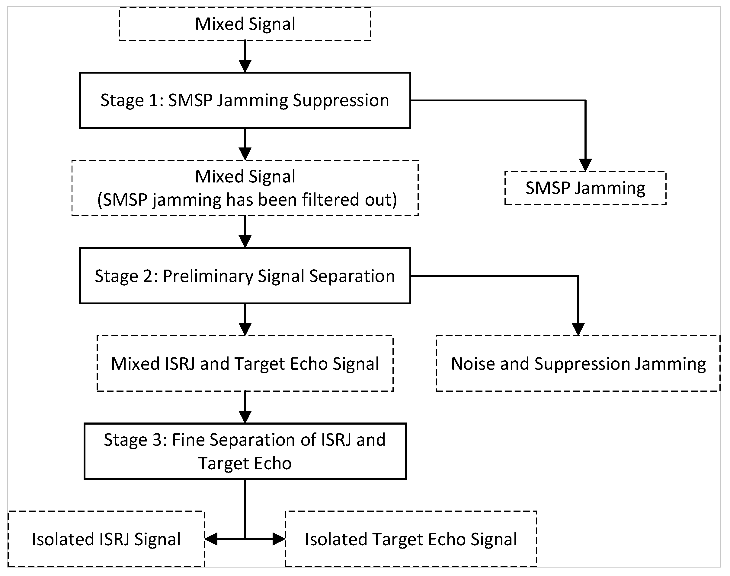
3. Signal Segregation and Key Time–Frequency Block Extraction for Hybrid Modality Fusion Network

This section aims to separate ISRJ signals and echo signals from complex electromagnetic environments. Subsequently, precise Region of Interest (ROI) [35] extraction is performed on the time–frequency maps of the separated ISRJ signals to facilitate the efficient deployment and operation of the HMFN.

3.1. Signal Separation

The overall signal separation process adopted in this paper is illustrated in Figure 7. This process progressively extracts the target signal and the ISRJ signal from mixed signal through three stages. In Stage 1, SMSP jamming is specifically suppressed. In Stage 2, background noise and various types of suppression jamming are further separated, yielding a mixed signal containing the ISRJ signal and the target echo. Finally, Stage 3 performs a fine separation on the mixture of the ISRJ signal and the target echo to obtain the ISRJ signal and the target echo signal, respectively.

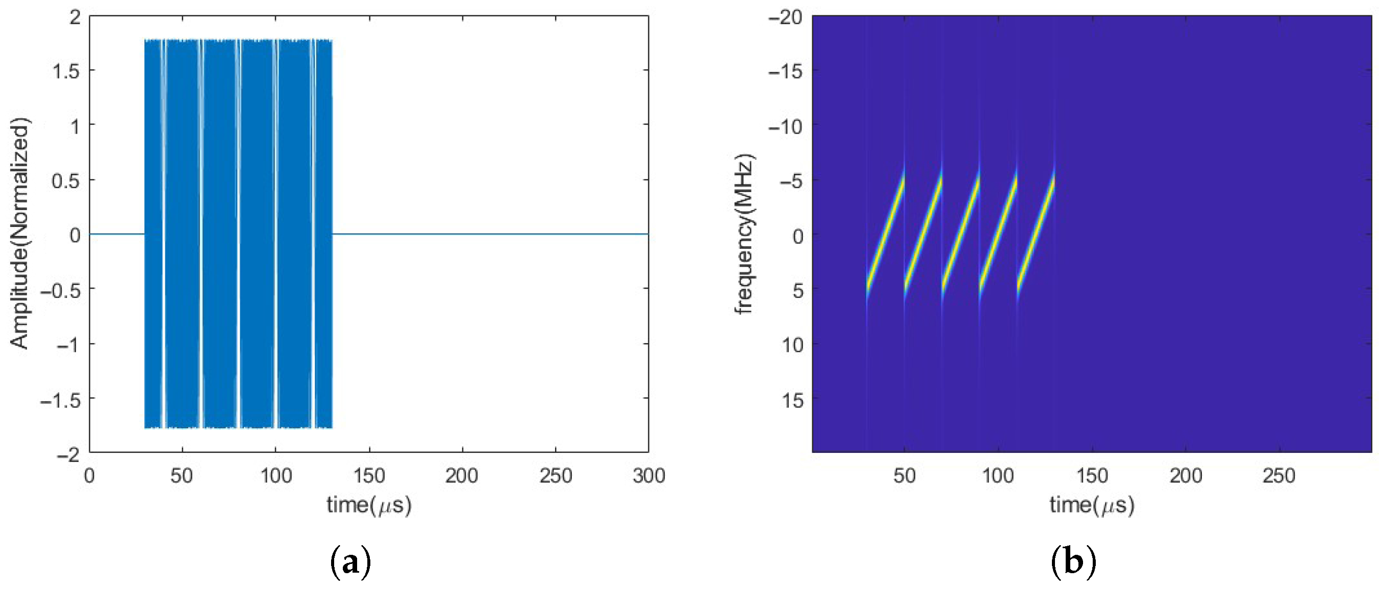
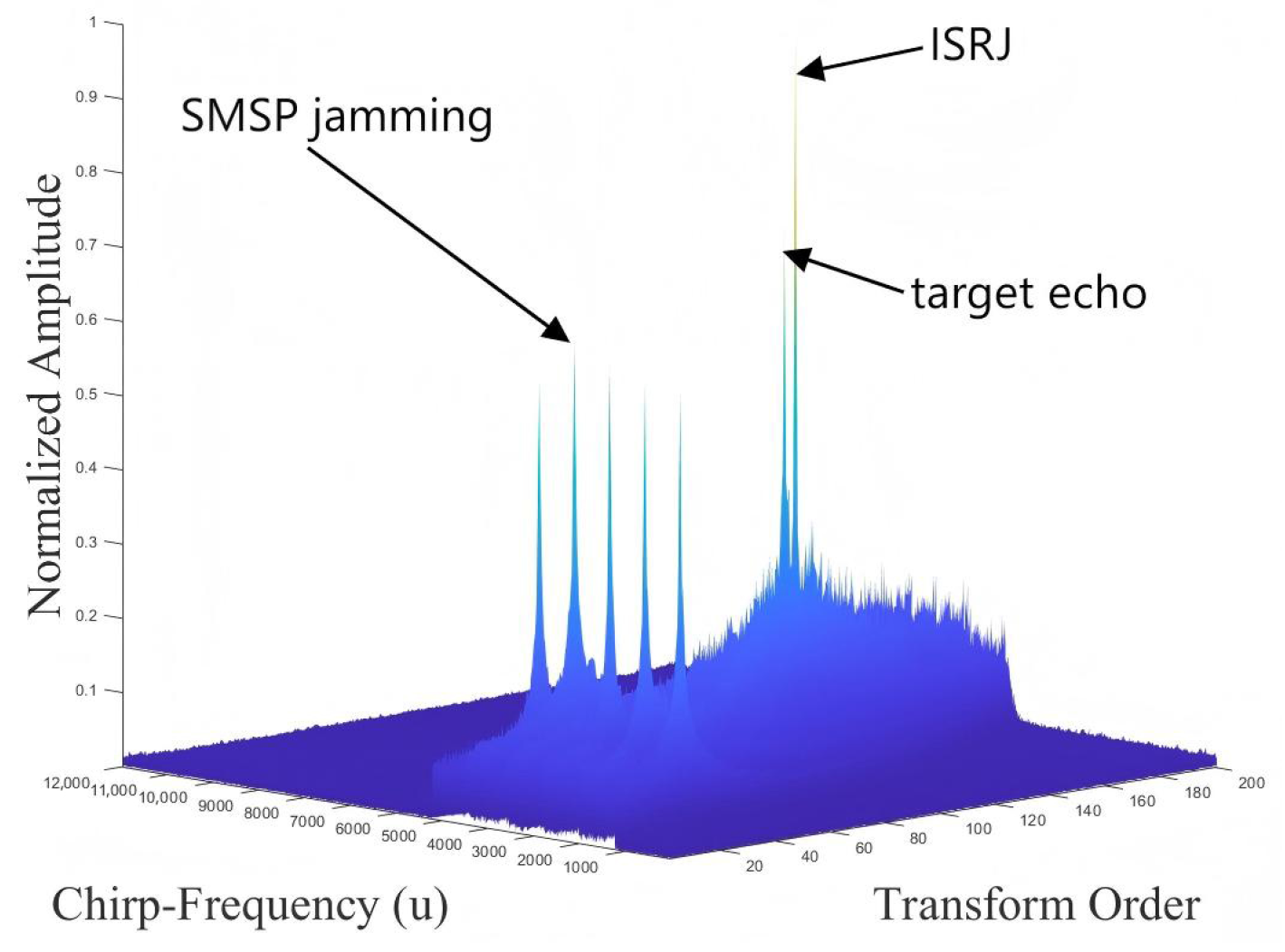
3.2. Feature Analysis of the Mixed Signal

Figure 8 illustrates the generation process of mixed signals in a battlefield environment. Importantly, by intercepting the radar’s transmitted signals and modulating them, the adversary can generate suppression jamming and deception jamming. Together with the true target echoes and background noise present in the environment, these components form the received mixed signal shown in the figure.

The mixed signal comprises true target echoes, two typical types of deception jamming (ISRJ and SMSP jamming), and suppression jamming (NCJ). The time-domain expression of this mixed signal can be modeled as follows:

$$r\left(t\right)=s_{\mathrm{echo}}\left(t\right)+s_{\mathrm{isrj}}\left(t\right)+s_{\mathrm{bj}}\left(t\right)+s_{\mathrm{smsp}}\left(t\right)+n\left(t\right)$$

(8)

where $r\left(t\right)$ represents the signal received by the receiver, $s_{\mathrm{echo}}\left(t\right)$ is the desired true target echo signal, $s_{\mathrm{isrj}}\left(t\right)$ and $s_{\mathrm{smsp}}\left(t\right)$ represent the two types of deception jamming signals, respectively, $s_{\mathrm{bj}}\left(t\right)$ represents the background suppression jamming, and $n\left(t\right)$ represents the background noise.

As shown in Figure 9a, when only the target echo and two types of deception jamming are present, the signal components already exhibit significant overlap in the time–frequency domain. Furthermore, Figure 9b shows the TFR of the mixed signal after the introduction of NCJ. It can be observed that the time–frequency structures of both the target echo and the deception jamming signals are almost completely masked by the strong suppression jamming. In this strong jamming environment, traditional signal-processing methods, such as time–frequency analysis and matched filtering, can hardly effectively extract useful information from the target echo or ISRJ jamming, leading to a severe degradation in the performance of target detection and jamming parameter estimation.

The concurrent presence of NCJ and SMSP poses distinct challenges to the processing of ISRJ signals. Specifically, the LFM structure of SMSP is similar to that of ISRJ sub-pulses, resulting in significant time–frequency overlap. This overlap complicates signal separation and introduces bias into the estimation of key ISRJ parameters. In contrast, NCJ acts as suppressive jamming that obscures the ISRJ’s time–frequency signature, as illustrated in Figure 9b. This masking effect, combined with the severe degradation in SNR, renders feature-based separation ineffective and parameter estimation unreliable. Consequently, a targeted, multi-stage suppression strategy is required to address these compound interferences.

Figure 10a clearly shows that in the range dimension, jamming signals generate numerous false peaks, resulting in dense false targets. Figure 10b further presents the outcome of applying Constant False Alarm Rate (CFAR) detection to the Range–Doppler (R-D) map from Figure 10a, where it is evident that these false targets are all confirmed as potential targets by the detection system. This observation highlights that without effective jamming suppression on the received signal, the radar will struggle to differentiate between true targets and false targets generated by jamming, thereby severely degrading its target detection performance and overall operational effectiveness.

To effectively separate the ISRJ signal and target echo signal, this paper introduces the FRFT [36] as a key processing tool. At a specific optimal order, the energy of an LFM signal becomes highly concentrated in the FRFT domain. This characteristic, combined with the linear superposition principle of FRFT, makes it possible to separate signal with different chirp rates in the FRFT domain. Figure 11 intuitively demonstrates the energy-focusing effect of FRFT on various components of the mixed signal.

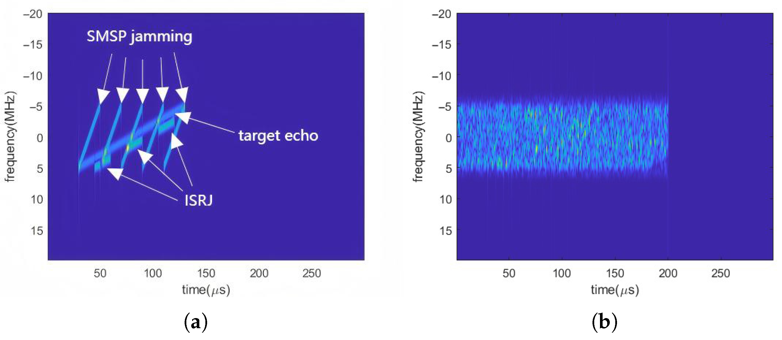
3.3. SMSP-Jamming Suppression Using FRFT

Before separating the target echo and ISRJ, to reduce the complexity of signal processing and improve subsequent separation performance, this paper introduces a preprocessing stage aimed at suppressing the SMSP jamming present in the mixed signal.

The SMSP jamming’s equivalent chirp rate ($K_{smsp}$) is an integer multiple ($n_{etc}$) of the radar’s chirp rate (K), allowing for a distinct optimal FRFT order $a_{smsp}$ where $K_{smsp}\approx K·n_{etc}$. To find the unknown $n_{etc}$, a search is performed over a candidate range (e.g., $[2,10]$). For each candidate $n_{etc}$, the corresponding $a_{smsp}$ is computed, and an FRFT is performed on the received signal $r\left(t\right)$. The $n_{etc}$ yielding the maximal energy concentration in the FRFT domain $R_{smsp}\left(u\right)$ is selected, and its associated $a_{smsp}$ is used for jamming suppression.

Transforming the received signal $r\left(t\right)$ into the $a_{smsp}$-order FRFT domain ($R_{smsp}\left(u\right)={\mathcal{F}}^{a_{smsp}}\left[r\left(t\right)\right]\left(u\right)$) concentrates the SMSP-jamming energy into distinct peaks, while the target echo and ISRJ energy remain dispersed due to the non-optimal order. A peak detection algorithm then identifies the jamming-energy region $U_{smsp}$ in $R_{smsp}\left(u\right)$. A binary mask $W_{smsp}\left(u\right)$ (near 0 in $U_{smsp}$, near 1 elsewhere) is applied to $R_{smsp}\left(u\right)$ to produce $R_{smsp}^{\prime }\left(u\right)=R_{smsp}\left(u\right)·W_{smsp}\left(u\right)$, selectively removing the jamming energy. Finally, an $a_{smsp}$-order Inverse FRFT (IFRFT) converts $R_{smsp}^{\prime }\left(u\right)$ back to the time domain signal $r^{\prime }\left(t\right)={\mathcal{F}}^{-a_{smsp}}\left[R_{smsp}^{\prime }\left(u\right)\right]\left(t\right)$. This significantly suppresses SMSP jamming in $r^{\prime }\left(t\right)$, facilitating subsequent target echo and ISRJ separation using their optimal FRFT order $a_{opt}$.

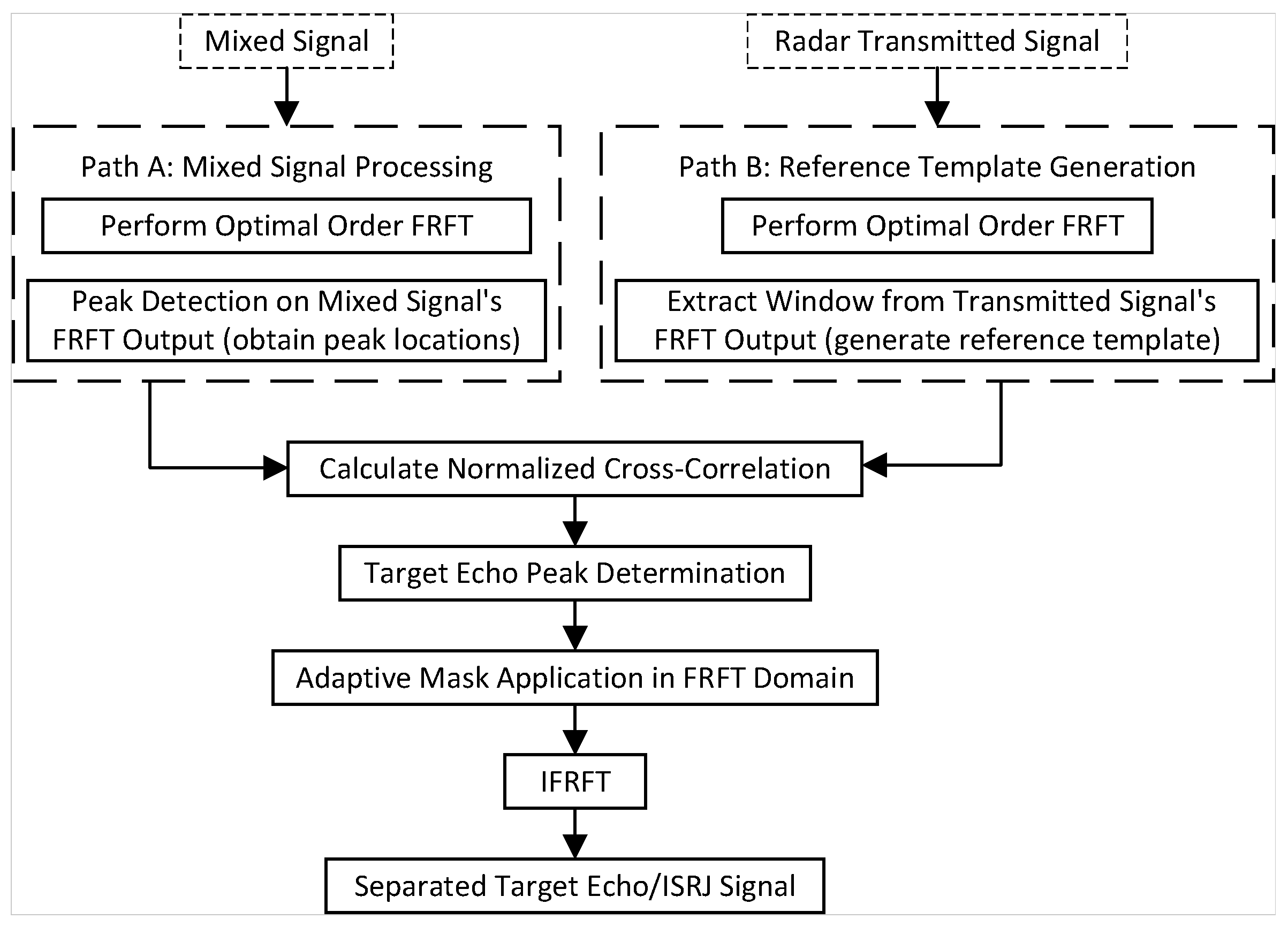
3.4. ISRJ and Echo Signal Separation

To further separate the ISRJ signal from the preprocessed mixed signal, this paper proposes an ISRJ signal separation method, as illustrated in Figure 12.

The algorithm illustrated in Figure 12 utilizes the inherent correlation between the target echo signal $s_{echo}\left(t\right)$ and the ISRJ signal $s_{isrj}\left(t\right)$. Typically, $s_{isrj}\left(t\right)$ and $s_{echo}\left(t\right)$ share a common chirp rate, leading to the same optimal FRFT order $a_{opt}$. Based on the linear superposition principle of the FRFT, the $a_{opt}$-order FRFT of the mixed signal, denoted as $R_{opt}\left(u\right)$ in the fractional domain u, can be approximated as follows:

$$\begin{array}{c}\hfill \begin{array}{cc}\hfill R_{\mathrm{opt}}\left(u\right)\approx & {\mathcal{F}}^{a_{\mathrm{opt}}}\left[s_{\mathrm{echo}}\left(t\right)\right]\left(u\right)+{\mathcal{F}}^{a_{\mathrm{opt}}}\left[s_{\mathrm{isrj}}\left(t\right)\right]\left(u\right)+{\mathcal{F}}^{a_{\mathrm{opt}}}\left[s_{\mathrm{bj}}\left(t\right)\right]\left(u\right)\hfill \\ \hfill & +{\mathcal{F}}^{a_{\mathrm{opt}}}\left[s_{\mathrm{smsp}}^{\prime }\left(t\right)\right]\left(u\right)+{\mathcal{F}}^{a_{\mathrm{opt}}}\left[n\left(t\right)\right]\left(u\right)|\hfill \end{array}\end{array}$$

(9)

where $s_{smsp}^{\prime }\left(t\right)$ represents the residual SMSP jamming. The optimal FRFT order $a_{opt}$ concentrates the energy of desired signals ($s_{echo}\left(t\right)$, $s_{isrj}\left(t\right)$) into peaks, while undesired components (suppression jamming $s_{bj}\left(t\right)$, residual SMSP $s_{smsp}^{\prime }\left(t\right)$, and noise $n\left(t\right)$) remain dispersed. This allows for their separation via fractional domain masking.

While both the target echo ($s_{echo}\left(t\right)$) and ISRJ ($s_{isrj}\left(t\right)$) share the same optimal FRFT order ($a_{opt}$), a challenge arises. Since the precise time delays of the echo and ISRJ segments are unknown, it is not possible to definitively associate specific peaks in $R_{opt}\left(u\right)$ with either the target echo or ISRJ components solely based on their positions.To address this ambiguity and correctly identify the echo signal, this paper employs a template matching approach. The FRFT of the known transmitted signal $s_{tx}\left(t\right)$ serves as a reference template, and the peak in $R_{opt}\left(u\right)$ exhibiting the highest shape similarity to this template is then identified as the target echo. The subsequent steps detail this distinction process.

1.

Reference Template Generation: The reference template $W_{ref}\left(u^{\prime }\right)$ is derived from the transmitted signal $s_{tx}\left(t\right)$. First, its $a_{opt}$-order FRFT-squared magnitude, $P_{ref}\left(u\right)={\left|{\mathcal{F}}^{a_{opt}}\left[s_{tx}\left(t\right)\right]\left(u\right)\right|}^2$, is computed. The template $W_{ref}\left(u^{\prime }\right)$ is then defined as a window of length L extracted from $P_{ref}\left(u\right)$, precisely centered at $P_{ref}\left(u\right)$’s main peak position $u_{tx}$, using a relative coordinate $u^{\prime }=u-u_{tx}$. L is chosen to encompass the main lobe and key side lobes, thereby capturing the characteristic peak shape.

2.

Peak Detection: Detect peaks in $R_{opt\_sq}\left(u\right)$ to obtain the peak positions $U=\{u_1,u_2,\dots ,u_M\}$.

3.

Template Matching: For each peak $u_i$ in $R_{opt\_sq}\left(u\right)$, centered at $u_i$, extract a window $W_i\left(u^{\prime }\right)$ of the same length L, where $u^{\prime }=u-u_i$. Calculate the Normalized Cross-Correlation [37] between $W_i\left(u^{\prime }\right)$ and the reference template $W_{ref}\left(u^{\prime }\right)$.

$$C_i={\displaystyle \frac{{\sum }_{u^{\prime }}{W}_i\left(u^{\prime }\right)W_{\mathrm{ref}}\left(u^{\prime }\right)}{\sqrt{{\sum }_{u^{\prime }}{W}_i{\left(u^{\prime }\right)}^2}\sqrt{{\sum }_{u^{\prime }}{W}_{\mathrm{ref}}{\left(u^{\prime }\right)}^2}}}$$

(10)

The range of $C_i$ is [−1, 1], where a value closer to 1 indicates higher shape similarity. The peak $u_i$ with the highest Normalized Cross-Correlation coefficient $C_i$ with the reference template $W_{ref}$ is selected and identified as the target echo peak $u_{echo}$.

4.

Time–Frequency Masking: After obtaining the peak position of the target echo, adaptive time–frequency masking is implemented to separate the ISRJ signal. The design of the mask $M(t,f)$ depends on the separation objective:

• Case 1: Separate and extract the ISRJ signal. Its definition is as shown in Equation (11):

$$\begin{array}{c}\hfill \begin{array}{c}\hfill M\left(u\right)=\left\{\begin{array}{cc}{M}_{\mathrm{suppression}}\left(u\right)\approx 0\hfill & \mathrm{if}u\in {\Omega }_{\mathrm{ECHO}}\hfill \\ M_{\mathrm{preservation}}\left(u\right)\approx 1\hfill & \mathrm{if}u\in {\Omega }_{\mathrm{ISRJ}}\hfill \end{array}\right.\end{array}\end{array}$$

(11)

where ${\Omega }_{\mathrm{ECHO}}$ represents the time–frequency region where the target echo signal is primarily distributed, and ${\Omega }_{\mathrm{ISRJ}}$ represents the time–frequency region where the ISRJ signal is primarily distributed.

• Case 2: Separate and extract the target echo signal. Its definition is as shown in Equation (12):

$$\begin{array}{c}\hfill \begin{array}{c}\hfill M\left(u\right)=\left\{\begin{array}{cc}{M}_{\mathrm{suppression}}\left(u\right)\approx 0\hfill & \mathrm{if}u\in {\Omega }_{\mathrm{ISRJ}}\hfill \\ M_{\mathrm{preservation}}\left(u\right)\approx 1\hfill & \mathrm{if}u\in {\Omega }_{\mathrm{ECHO}}\hfill \end{array}\right.\end{array}\end{array}$$

(12)

This mask $M(t,f)$ is applied to the FRFT representation $S(t,f)$ of the original signal to obtain the processed time–frequency distribution $Y\left(u\right)$:

$$Y\left(u\right)=R_{opt}\left(u\right)\odot M\left(u\right)$$

(13)

Subsequently, the time-domain signal $s_y\left(t\right)$ is reconstructed from $Y\left(u\right)$ through an IFRFT. The signal $s_y\left(t\right)$ will primarily contain the desired signal component (either the ISRJ signal or the target echo), while the other signal component is effectively suppressed, thus achieving selective separation of the two types of signals.

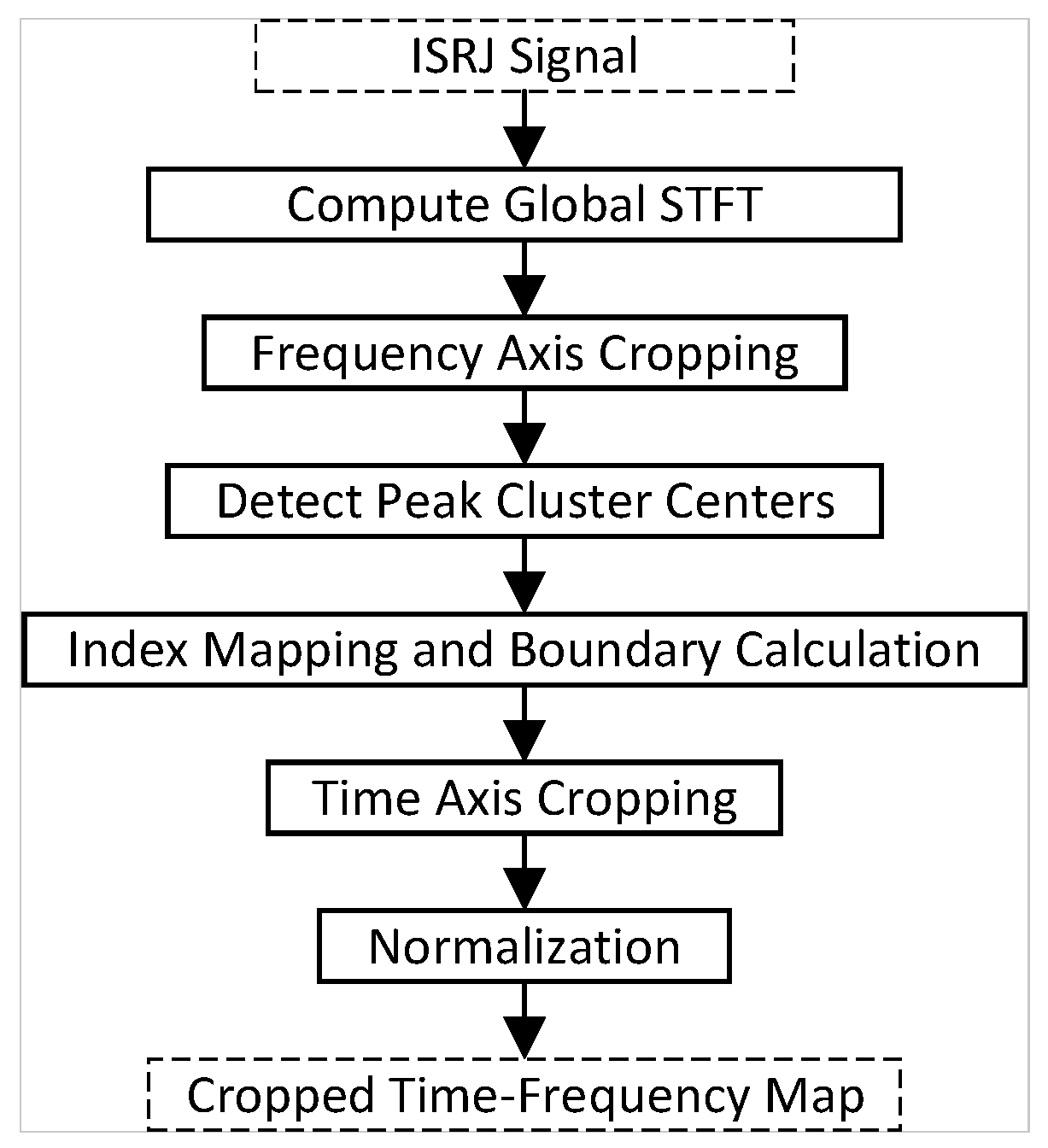
3.5. Time–Frequency Region of Interest Extraction

ISRJ signals typically exhibit sparsity in the time–frequency domain, with their effective information occupying only a small portion of the time–frequency map. To reduce the computational complexity of subsequent parameter estimation, this paper proposes an adaptive cropping method in the time–frequency domain guided by matched filtering, aiming to accurately extract useful signal components from the time–frequency map. The processing flow is illustrated in Figure 13, and the specific steps are as follows:

1.

Global STFT Calculation: Perform STFT on the ISRJ signal $s_{\mathrm{isrj}}\left[n\right]$ to obtain the global time–frequency spectrum $S_{\mathrm{isrj}}(m,f)$.

2.

Frequency axis cropping: Given that the bandwidth $B_S$ of the ISRJ signal is usually narrower than the bandwidth $B_{tx}$ of the radar-transmitted signal, first perform frequency axis cropping on the global time–frequency spectrum $S_{\mathrm{isrj}}(m,f)$ based on the spectral range of the radar-transmitted signal ($f_{\mathrm{start}}$ and $f_{\mathrm{stop}}$).

3.

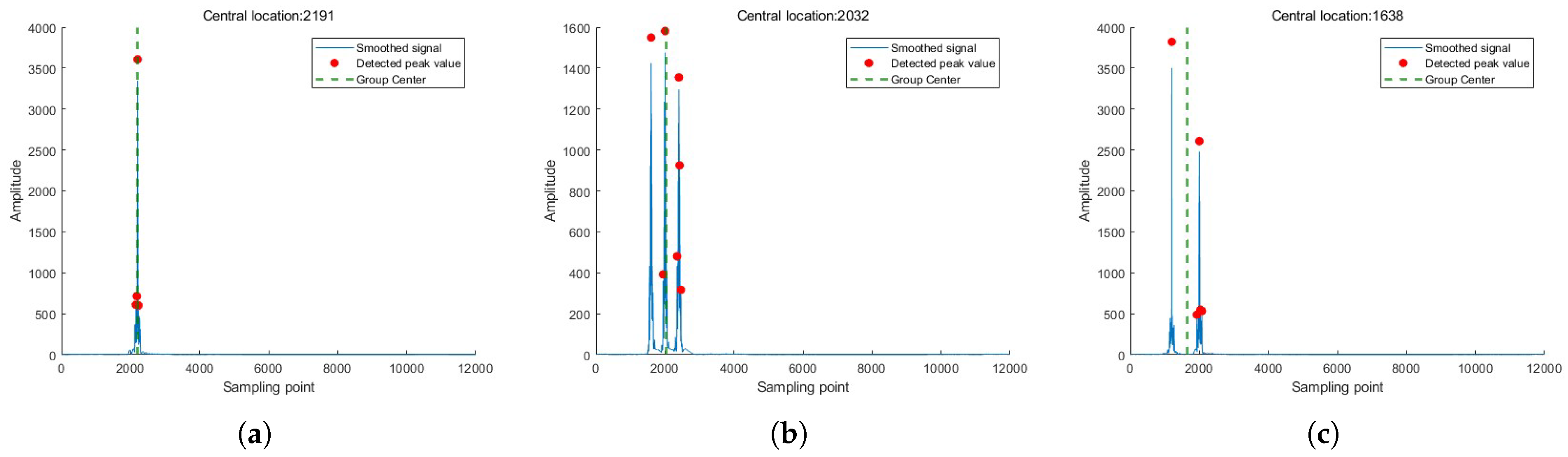
Peak Cluster Center Detection: To locate the active intervals of the signal on the time axis, perform matched filtering on the ISRJ signal $s_{\mathrm{isrj}}\left[n\right]$ to obtain the output $s_y\left[n\right]$. Then, apply a peak cluster center detection algorithm to its magnitude $|s_y\left[n\right]|$. This detection integrates signal smoothing [38], adaptive threshold setting, multi-conditional peak screening, and cluster center calculation [39], thereby robustly estimating the core regions of signal energy on the time axis of the matched filter output.

4.

Index Mapping and Calculation: Map the peak cluster centers from the time axis of the matched-filter output to the time axis of the STFT.

5.

Time Axis Cropping: Based on the calculated $m_{\mathrm{start}}$ and $m_{\mathrm{stop}}$, perform time-axis cropping on the frequency-cropped time–frequency matrix $S_{\mathrm{freq\_crop}}$ to extract the time–frequency representation $S_{\mathrm{tf\_crop}}(m^{\prime },k^{\prime })$ of the region where the jamming signal primarily exists:

$$S_{\mathrm{tf\_crop}}(m^{\prime },k^{\prime })=S_{\mathrm{freq\_crop}}(m_{\mathrm{start}}+m^{\prime }-1,k^{\prime }),m^{\prime }=1,\dots ,(m_{\mathrm{stop}}-m_{\mathrm{start}}+1)$$

(14)

6.

Standardized Output: To facilitate use by subsequent processing modules, the cropped time–frequency matrix $S_{\mathrm{tf\_crop}}$ is embedded into the center of a predefined fixed-size matrix through zero-padding, resulting in a standardized-size output, $cropped\_signal$.

4. ISRJ Signal Sampling Duration Estimation Based on Hybrid Modality Fusion Network

In Section 3, this paper achieved the separation of the ISRJ signal from the mixed signal. However, the performance of signal separation degrades when the SJR decreases. This degradation may lead to varying degrees of distortion in the separated ISRJ signal. To mitigate the impact of signal distortion on parameter estimation, this section proposes an HMFN based on Multi-feature Fusion [40]. This network integrates signal information beyond the time–frequency domain through feature fusion to enhance the robustness of parameter estimation.

4.1. Feature Extraction

To construct a feature vector that can comprehensively characterize the properties of ISRJ signals and exhibit a certain degree of robustness to spectrogram distortions, this paper extracts ISRJ signal features from the following three aspects: The dual-path feature extraction is designed for informational complementarity. While matched filtering is ideal for extracting pulse-related structural features due to its SNR gain, it can alter the signal’s intrinsic statistical profile. The raw signal path therefore preserves these crucial statistics, such as skewness and kurtosis, which characterize the overall signal environment. Fusing these two complementary feature sets yields a more robust and discriminative vector for the subsequent estimation task.

4.1.1. ISRJ Time-Domain Waveform Feature Extraction

1.

Basic Statistical Features: Calculate the mean, median, variance, skewness, kurtosis, and maximum value of the envelope $\left|s\right(t\left)\right|$. These statistics describe the central tendency, dispersion, shape, and peak level of the amplitude distribution.

2.

Signal Activity and Variability Features: Extract the duty cycle of the amplitude (reflecting signal activity or intermittency), the rate of amplitude change (characterizing the rate of change and fluctuation of the envelope), and the crest factor (measuring the prominence of peaks).

3.

Energy and Sparsity Features: Calculate the average power of the signal (characterizing the average energy level), the power spectral entropy (reflecting the concentration of energy in the time domain), and the L1/L2 norm ratio (measuring the sparsity of the signal).

4.

Amplitude Autocorrelation Features: Extract the position of the first significant non-zero delay peak of the normalized autocorrelation function of $\left|s\right(t\left)\right|$. This feature helps capture the periodicity or repetitive patterns of the envelope and plays an auxiliary role in distinguishing different forwarding modes.

4.1.2. Time-Domain Feature Extraction of ISRJ Signal After Matched Filtering

Matched filtering is applied to the ISRJ signal $s\left(t\right)$ to enhance its pulse structure characteristics, resulting in $s_{MF}\left(t\right)$.

1.

Pulse Peak Characteristic Statistics: First, detect all pulse peaks in the amplitude envelope $|s_{MF}\left(t\right)|$ and record their total number. Second, for the amplitudes of the detected peaks, calculate their mean, median, standard deviation, and maximum value to quantify the statistical distribution characteristics of pulse intensity.

2.

Pulse Repetition Interval [41] Statistical Analysis: Extract the sequence of time intervals between adjacent pulse peaks and calculate the mean, median, standard deviation, minimum, and maximum values of this sequence. These statistics aim to characterize the pulse repetition time structure of the ISRJ signal.

3.

Pulse Peak Position Distribution Features: Calculate the standard deviation of the occurrence times of all detected pulse peaks. This value is used to measure the dispersion of pulses on the time axis. Additionally, determine the precise time positions of the first and last pulse peaks to define the duration range of the entire effective pulse sequence.

4.

Macroscopic Characteristics of the Amplitude Envelope After Matched Filtering: Calculate the mean of the amplitude envelope $|s_{MF}\left(t\right)|$ as an indicator of the overall energy or average intensity of the signal after matched filtering. Simultaneously, extract the position of the first significant non-origin peak of its normalized autocorrelation function to detect the macroscopic periodic structure of the amplitude envelope after matched filtering.

4.1.3. Jamming-Type Encoding

To integrate prior knowledge of jamming types, this paper adopts a one-hot encoding scheme to numerically represent the jamming types. This encoding method ensures that the neural network can effectively utilize this categorical information while avoiding the misinterpretation of class labels as ordinal numerical values.

Finally, the 14 feature parameters extracted from the original time-domain signal and the 15 feature parameters from the matched-filtered signal are concatenated and fused with the corresponding 3-bit one-hot encoded vector of the jamming type to form a 32-dimensional comprehensive feature vector. This vector aims to characterize the key properties of the ISRJ signal from multiple dimensions and will be directly used as input to the proposed HMFN to achieve high-precision estimation of the ISRJ-signal-sampling duration parameter.

These handcrafted features constitute one of two parallel processing paths within our HMFN. This dual-path architecture is designed to fuse complementary information sources. While a CNN excels at extracting localized patterns, its ability to discern global statistical properties diminishes when the time–frequency map is degraded by significant noise. The features detailed in this section are engineered to explicitly capture these very properties.

The selection of these features is therefore not arbitrary but is rooted in the physical signature of ISRJ. They quantify the signal’s core characteristics from three complementary perspectives: (1) its intermittent, non-Gaussian statistical distribution (e.g., kurtosis); (2) its underlying structural periodicity (e.g., autocorrelation peaks), which directly relates to the jammer’s timing; and (3) its energy fluctuation (e.g., spectral entropy), resulting from the on–off switching. Although minor correlations among some indicators are expected, the feature set as a whole provides a multi-faceted and largely non-redundant signal “fingerprint.” Fusing this explicit, expert-driven knowledge from the Multi-Layer Perceptron (MLP) branch with the implicit, data-driven patterns from the CNN branch allows the HMFN to construct a far more robust and comprehensive signal representation, thereby mitigating the risks associated with a single-modality approach.

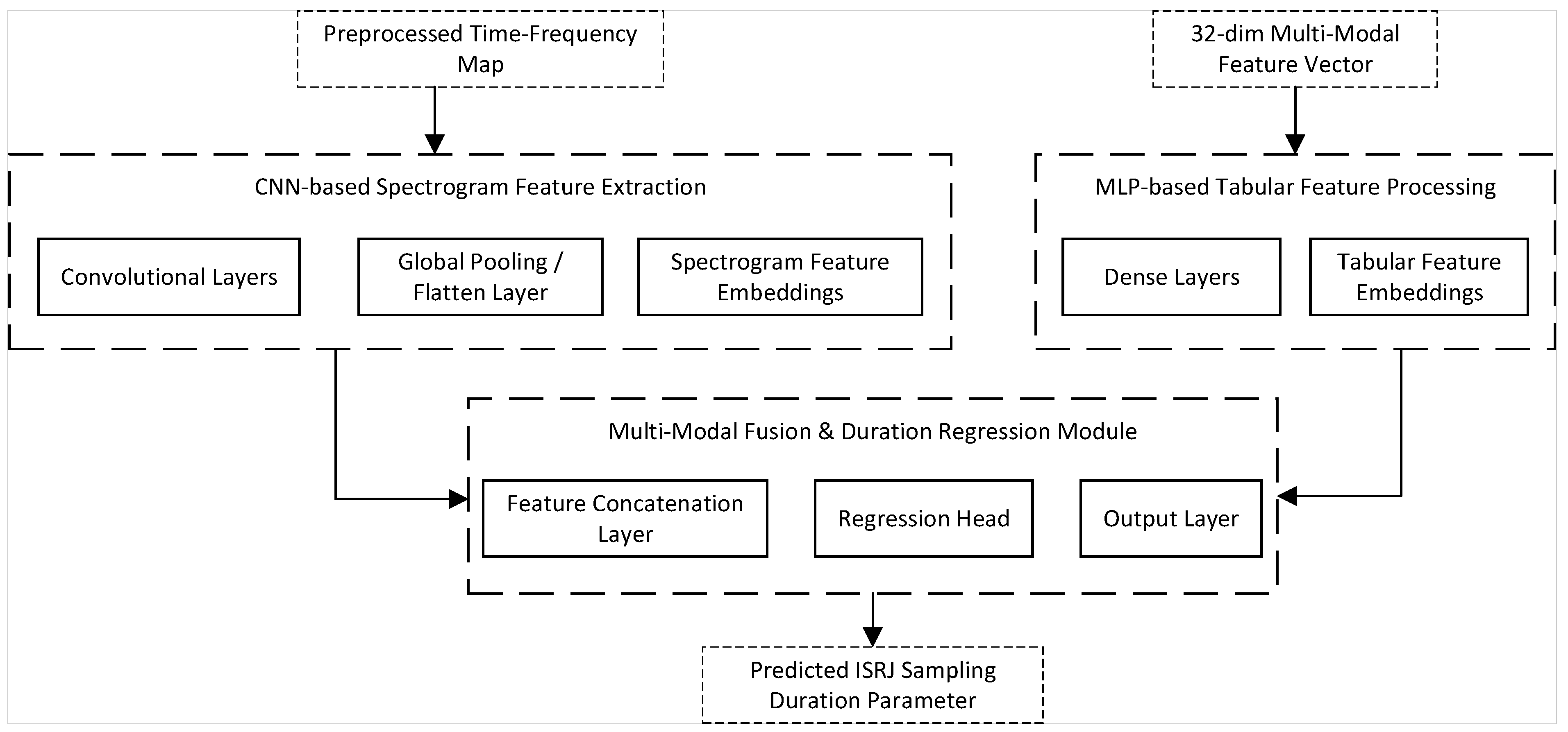
4.2. Hybrid Modality Fusion Network

This paper proposes a hybrid deep learning architecture, named the Hybrid Modality Fusion Network, whose overall structure is shown in Figure 14. The HMFN employs a dual-branch parallel processing mechanism, dedicated to constructing an accurate non-linear mapping from raw multi-modal observation data to the ISRJ-signal-sampling duration, with the goal of overcoming the performance bottlenecks of traditional parameter estimation methods.

To achieve a comprehensive characterization of ISRJ, the HMFN model utilizes two input data modalities with significant complementarity:

• Time–Frequency Representation and Convolutional Feature Extraction: This paper selects the spectrogram as a core input branch for the network to capture the dynamic details of the signal spectrum evolving over time [42]. This high-dimensional time–frequency representation is fed into a convolutional neural network (CNN) module, which, through its hierarchical feature learning capability, can adaptively extract and encode complex time–frequency patterns sensitive to the sampling duration.
• Explicit Incorporation of Feature Vectors and A Priori Knowledge: The model additionally integrates a low-dimensional feature vector $X_{feat}$. It provides a physically meaningful and compact representation of the signal’s key physical attributes, especially those directly reflecting sampling behavior. The introduction of such features helps compensate for information loss due to spectrogram distortion. More critically, this a priori knowledge, directly related to the sampling duration, can guide the model, making its learning process more focused on the accurate estimation of the target parameter.

The architecture primarily comprises three key parts: the CNN Feature Extraction Module, the MLP Feature Vector Processing Module, and the Feature Fusion and Regression Prediction Module.

• CNN Feature Extraction Module: This module processes the high-dimensional TFR input $X_{TFR}$. Its core is a CNN-processing unit. This unit typically consists of stacked convolutional layers, non-linear activation functions, batch normalization layers [43], and pooling layers. Convolutional layers utilize learned convolutional kernels to extract patterns with local time–frequency characteristics. After passing through the CNN-processing unit and subsequent global pooling and flattening operations, the high-dimensional time–frequency feature map is ultimately mapped to a fixed-dimension time–frequency latent feature vector. This vector can be regarded as a projection of the original spectrogram into a latent semantic space highly relevant to the sampling duration prediction task.
• MLP Feature Vector Processing Module: As indicated in the “MLP-based Tabular Feature Processing” part of Figure 14, this module receives the low-dimensional engineered feature vector $X_{feat}$. Its core is an MLP-processing unit. This unit is composed of multiple fully connected layers, non-linear activation functions, and batch normalization layers, supplemented by Dropout regularization [44]. This module ultimately outputs a fixed-dimension engineered feature latent vector $f_{feat}\in {\mathbb{R}}^{B\times 64}$. Its dimension is carefully designed for effective fusion with the time–frequency features $f_{TFR}$ extracted by the CNN.
• Feature Fusion and Regression Prediction Module: This module integrates heterogeneous features from the preceding parallel branches and outputs the estimated ISRJ sampling duration. As shown in Figure 14, first, the time–frequency latent feature vector $f_{TFR}$ output by the CNN module and the engineered feature latent vector $f_{feat}$ output by the MLP module are concatenated along the feature dimension. This forms a higher-dimensional fused feature vector $f_{fused}$. Subsequently, the fused feature vector $f_{fused}$ is fed into a regression head for processing. The regression head internally contains a regression-processing unit. Its role is to perform further non-linear transformations and information refinement on the fused high-dimensional features to extract the final abstract representation most relevant to the target prediction. Finally, through an output layer, this final feature representation is mapped to the target prediction value, i.e., the predicted sampling duration of the ISRJ signal $\widehat{y}$.

In summary, this section has detailed a hybrid deep learning framework designed for the precise estimation of ISRJ sampling duration. Its core strategy involves the following: utilizing a CNN to extract deep time–frequency structural features from high-dimensional time–frequency representations while concurrently employing an MLP to process low-dimensional engineered feature vectors containing a priori knowledge. Subsequently, these two complementary heterogeneous features are effectively fused and input into the final regression prediction module. This framework aims to construct a high-precision, robust, non-linear mapping model from multi-modal raw observations to the ISRJ-sampling duration, with the goal of overcoming the performance bottlenecks faced by traditional methods in this task.

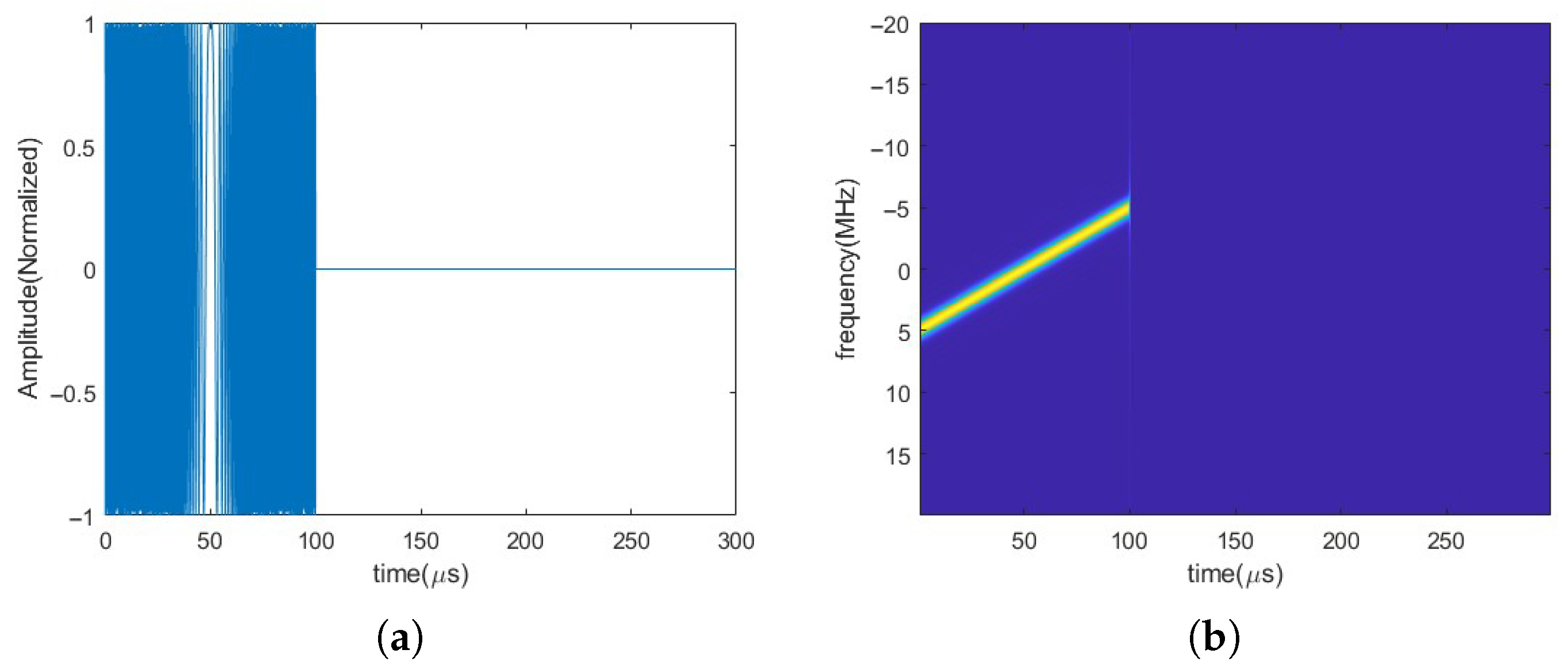
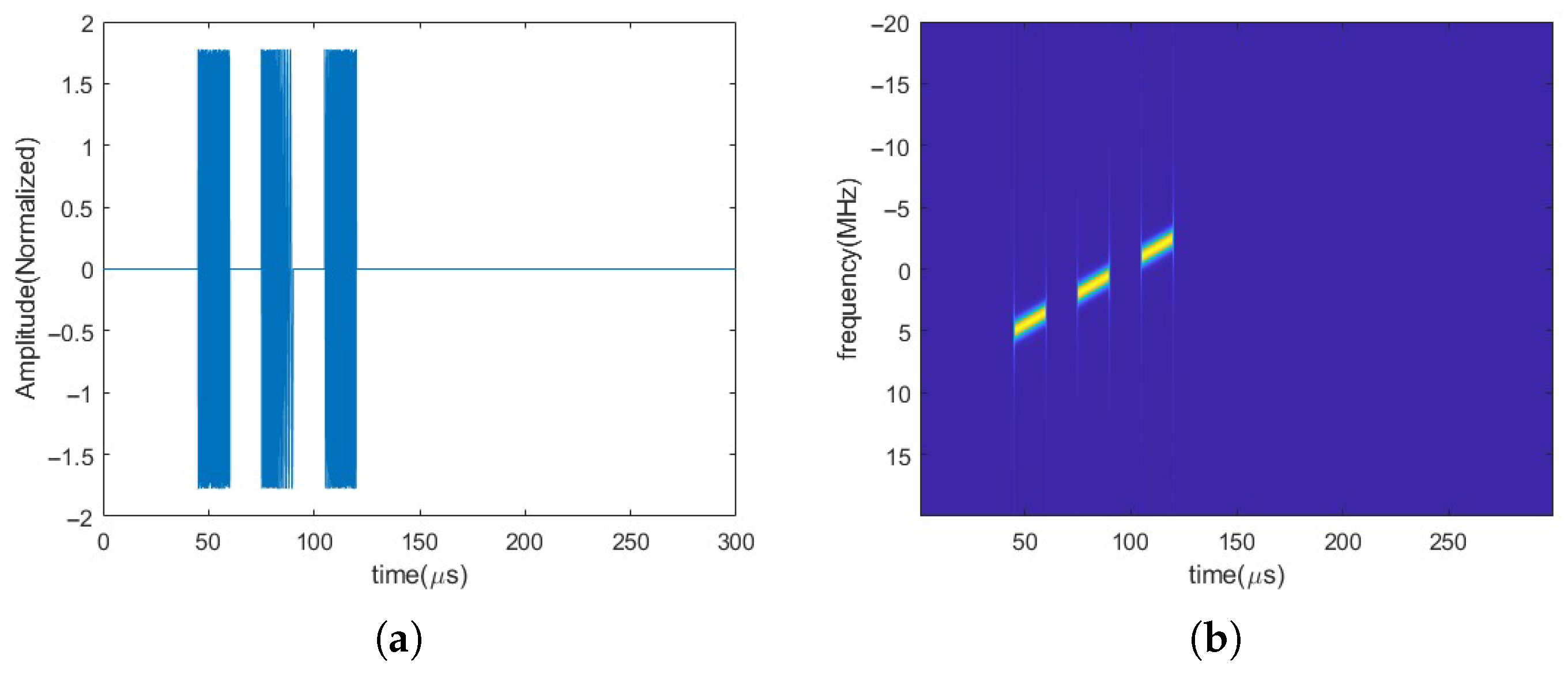
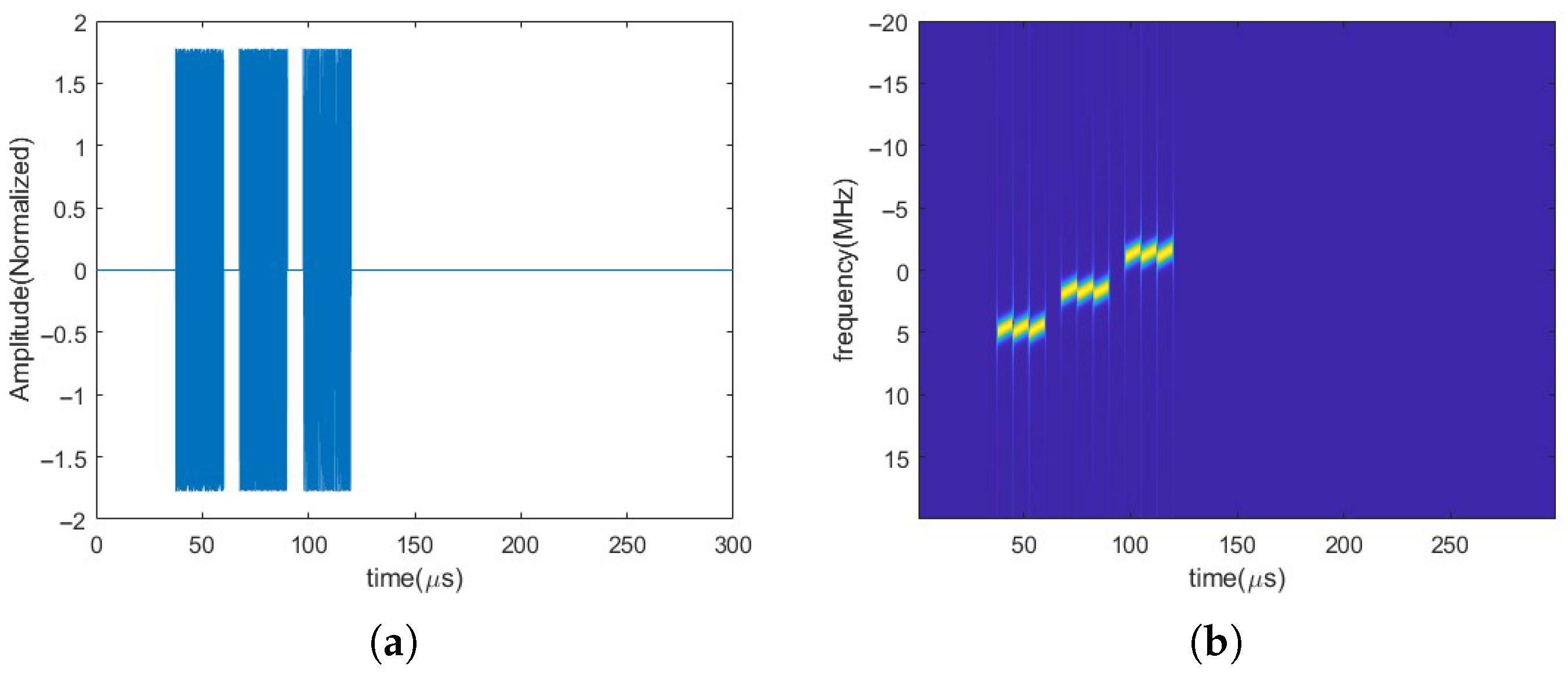
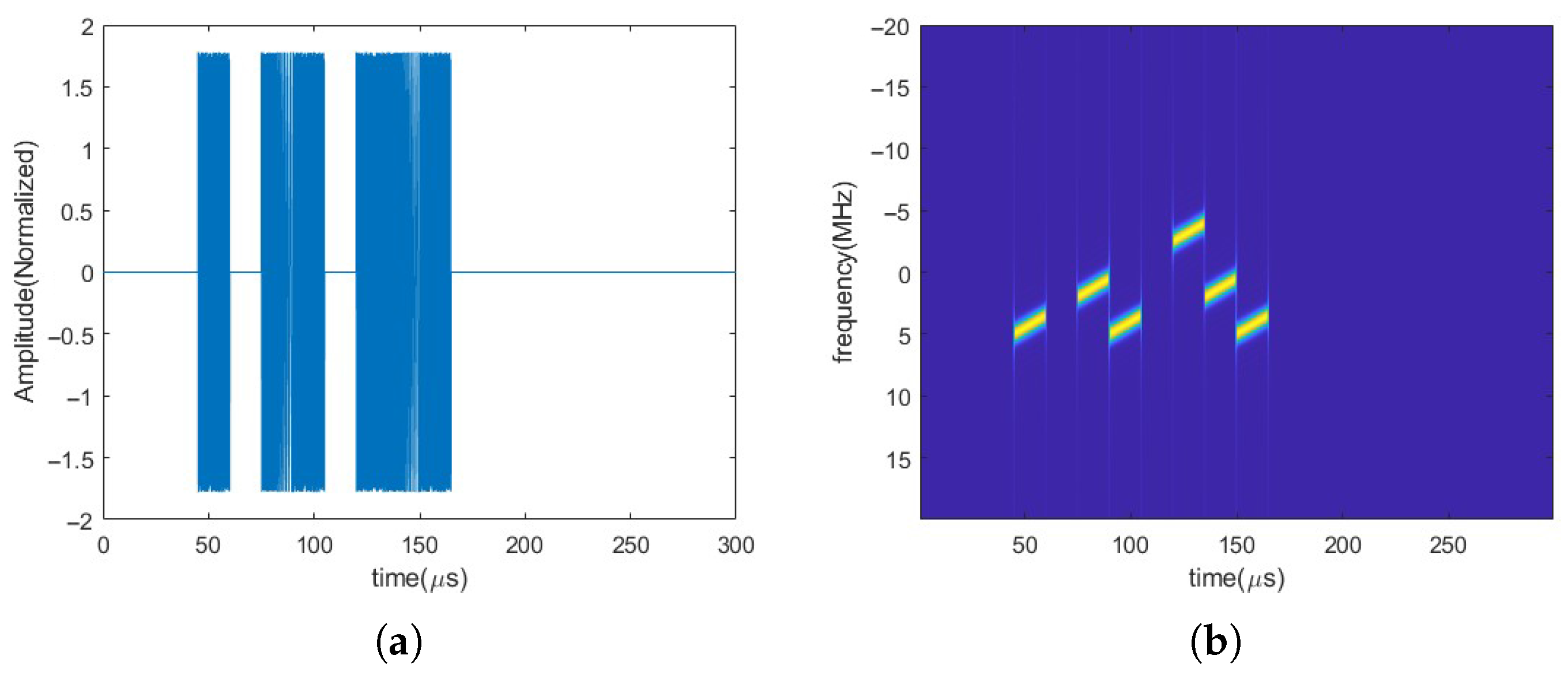
5. Simulation Analysis

To validate the effectiveness of the proposed method regarding mixed-signal separation, time–frequency map cropping, and parameter estimation, numerical simulations were conducted. The specific parameter settings for these simulations are detailed in

Table 1. Signal parameters.

Parameter	Value
Radar-transmitted-signal pulse width	100 $\mathsf{\mu }\mathrm{s}$
Radar-transmitted-signal bandwidth	10 MHz
Radar-transmitted-signal chirp rate	100 GHz
Sampling rate	40 MHz
ISDRJ-sampling-duration range	10–50 $\mathsf{\mu }\mathrm{s}$
ISPRJ-sampling-duration range	5–25 $\mathsf{\mu }\mathrm{s}$
ISCRJ-sampling-duration range	5–25 $\mathsf{\mu }\mathrm{s}$
SMSP-jamming decimation factor range	2–8
SNR	5 dB
SJR (Deception Jamming)	−5 dB
SJR (Suppression Jamming)	−8 dB

.

5.1. Mixed-Signal Separation

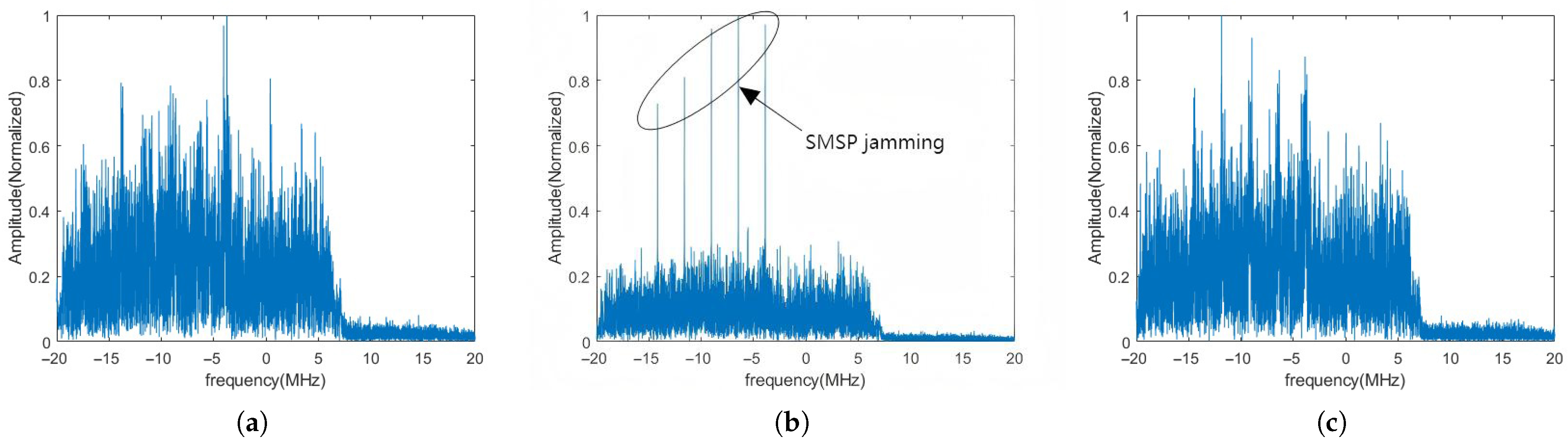
5.1.1. SMSP Jamming Filtering

Figure 15 shows the optimal order FRFT performed assuming the chirp rate of the SMSP jamming is different integer multiples of the echo signal’s chirp rate. Using the method described in Section 3, the multiplication factor of this SMSP jamming can be identified as 5, thereby determining the chirp rate of the SMSP jamming.

By zeroing out or attenuating the energy-concentrated regions in Figure 15b and then performing an inverse FRFT, the SMSP jamming can be effectively filtered out. Figure 16 shows the time–frequency representation of the mixed signal after applying this processing method.

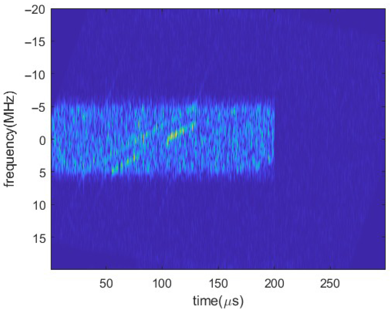
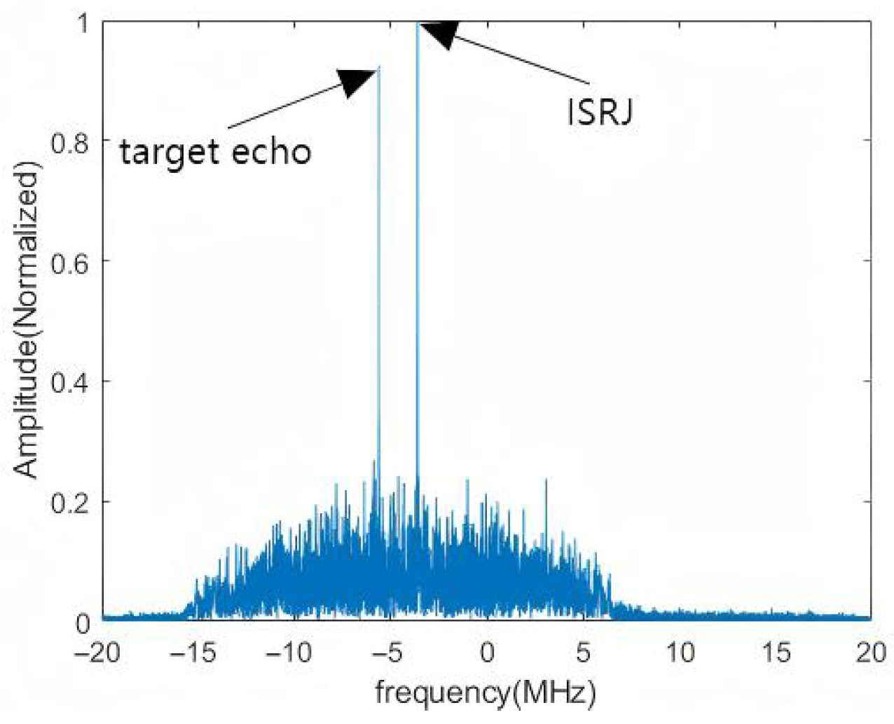
5.1.2. Extraction of ISRJ and Target Echo Signal

Figure 17 shows the result of performing FRFT on the mixed signal at the optimal order. The energy of the ISRJ and echo signal is effectively concentrated in the optimal fractional domain, manifesting as sharp peaks. By using the template-matching method described in Section 3 to distinguish between the echo signal and the ISRJ, and then applying a time–frequency mask, separate extraction of both signals can be achieved.

Figure 18 shows the TFRs of the target echo signal and the ISRJ separated from the mixed signal. Specifically, Figure 18a presents the spectrogram of the target echo signal, while Figure 18b corresponds to the spectrogram of the ISRJ.

To assess the algorithm’s robustness against background noise, a critical factor in practice, we evaluated its performance under varying SNRs while holding jamming SJRs constant. Figure 19 shows the TFR of the separated signal (ISRJ) at several challenging SNR levels. At 5 dB SNR (Figure 19a), the signal components are distinct against a clean background. As SNR drops to 0 dB (Figure 19b), the noise floor rises, yet the signal’s core LFM structure remains well-preserved. Even in the severe −5 dB SNR case (Figure 19c), where the signal is partially submerged in heavy noise, its energy is still concentrated along the characteristic chirp-rate line. The preservation of these fundamental features confirms that the separated signal is a viable input for the subsequent HMFN, underscoring the strong noise resilience of our FRFT-based method.

Different types of ISRJ exhibit significant differences in the time-frequency domain. To evaluate the signal separation performance of the proposed method for various ISRJ types, corresponding experiments were conducted. Figure 20 show the separation results for three types of ISRJ. As shown in the figure, although different types of ISRJ possess distinct time-frequency structures, the proposed separation algorithm can effectively and accurately separate the ISRJ components from the mixed signal.

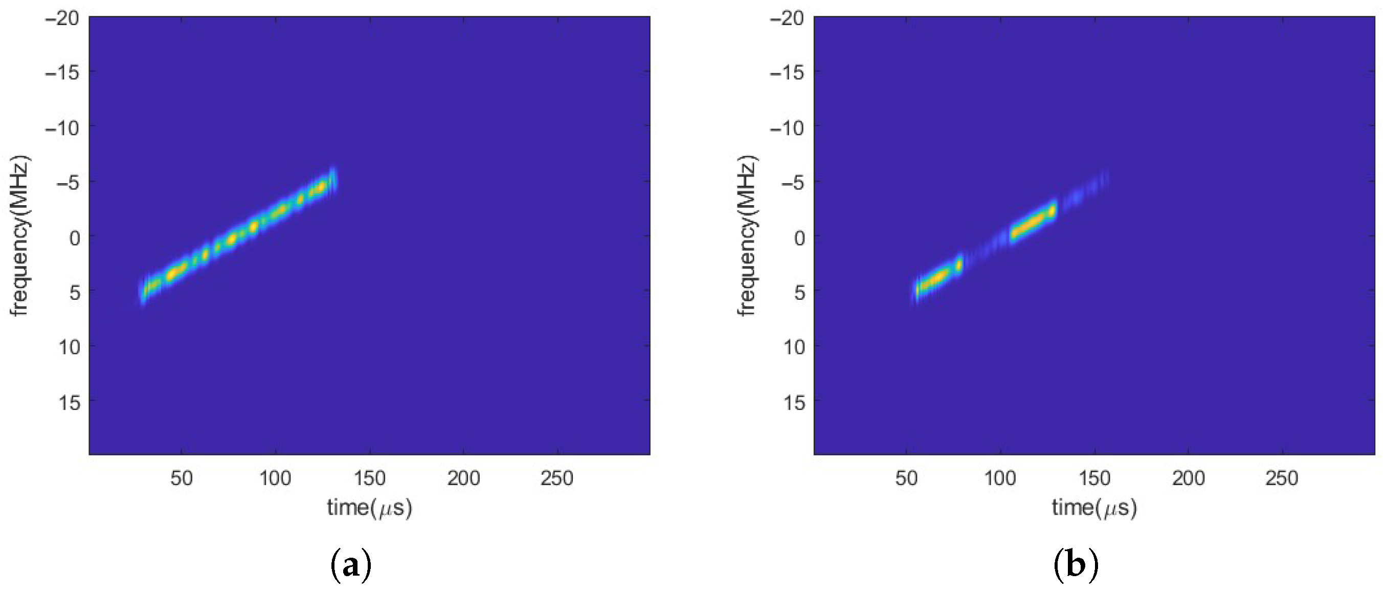
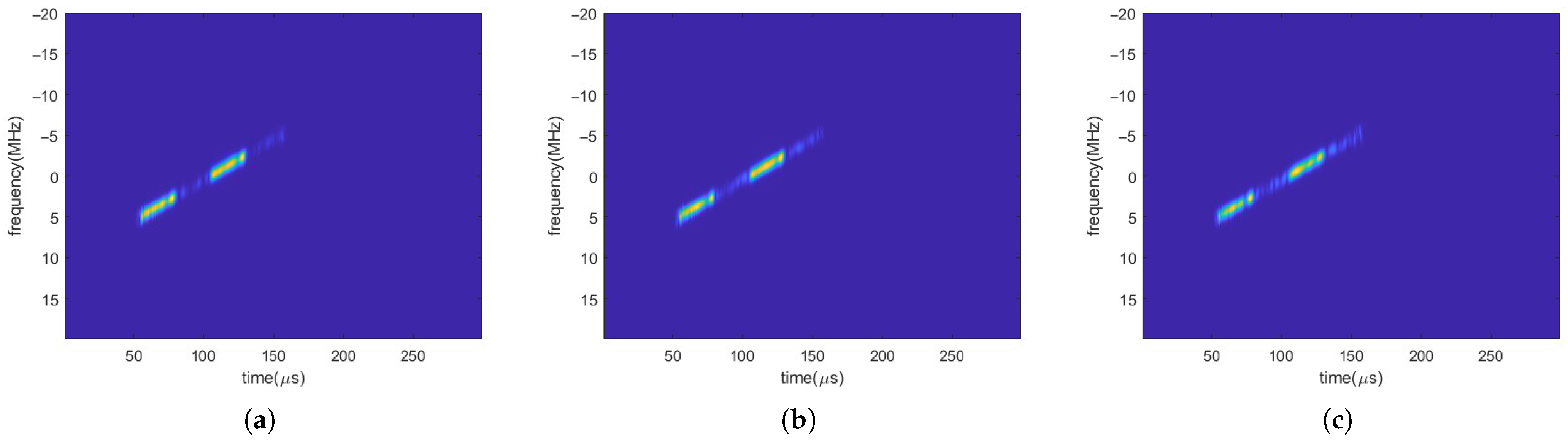
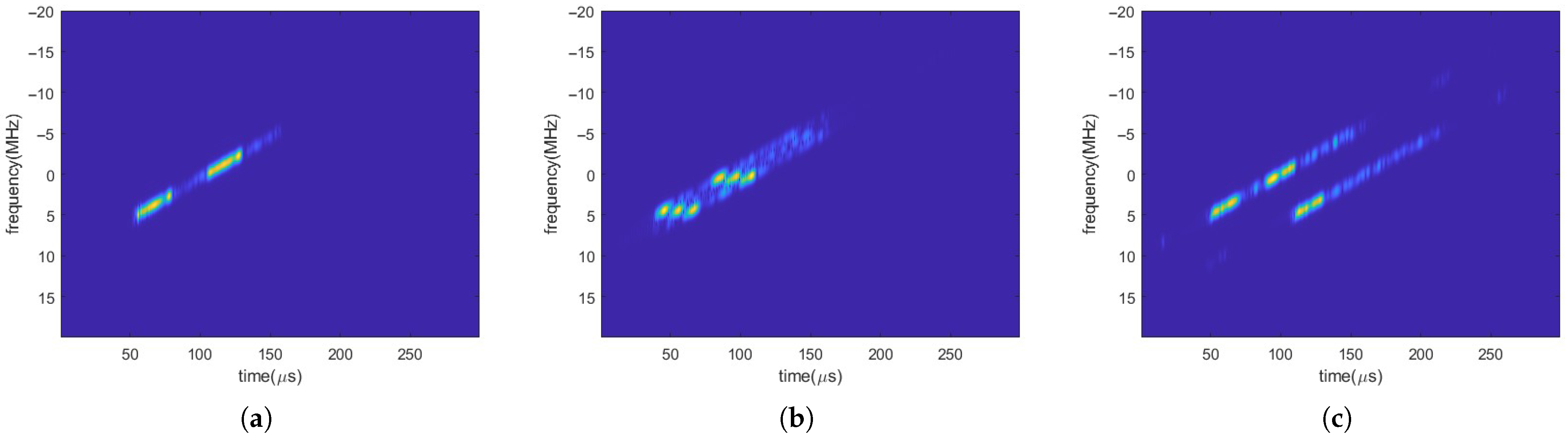
5.1.3. Time–Frequency Map Cropping

Figure 21 shows the results of peak cluster center detection on the pulse compression images of three ISRJ subtypes. For the main components in the ISRJ spectrogram, this method identifies the region containing the primary signal content, and the spectrogram is then cropped accordingly.

Figure 22 shows the cropped spectrograms, where subfigures a-c correspond to ISDRJ, ISPRJ, and ISCRJ respectively. Their dimensions were reduced from 512 × 184 to 148 × 100, thereby significantly decreasing the spectrogram size. For the proposed network, the computational load after cropping was reduced to less than one-sixth of its original level.This cropping leads to a significant reduction in network training and inference times.

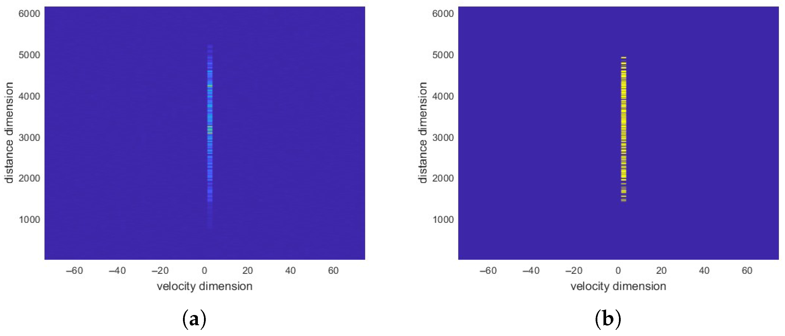
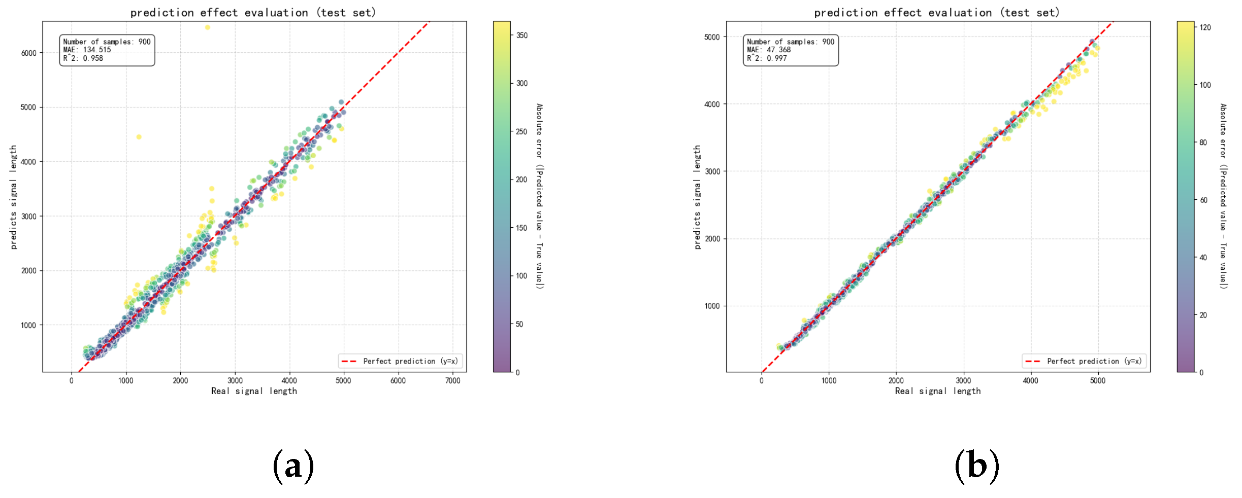
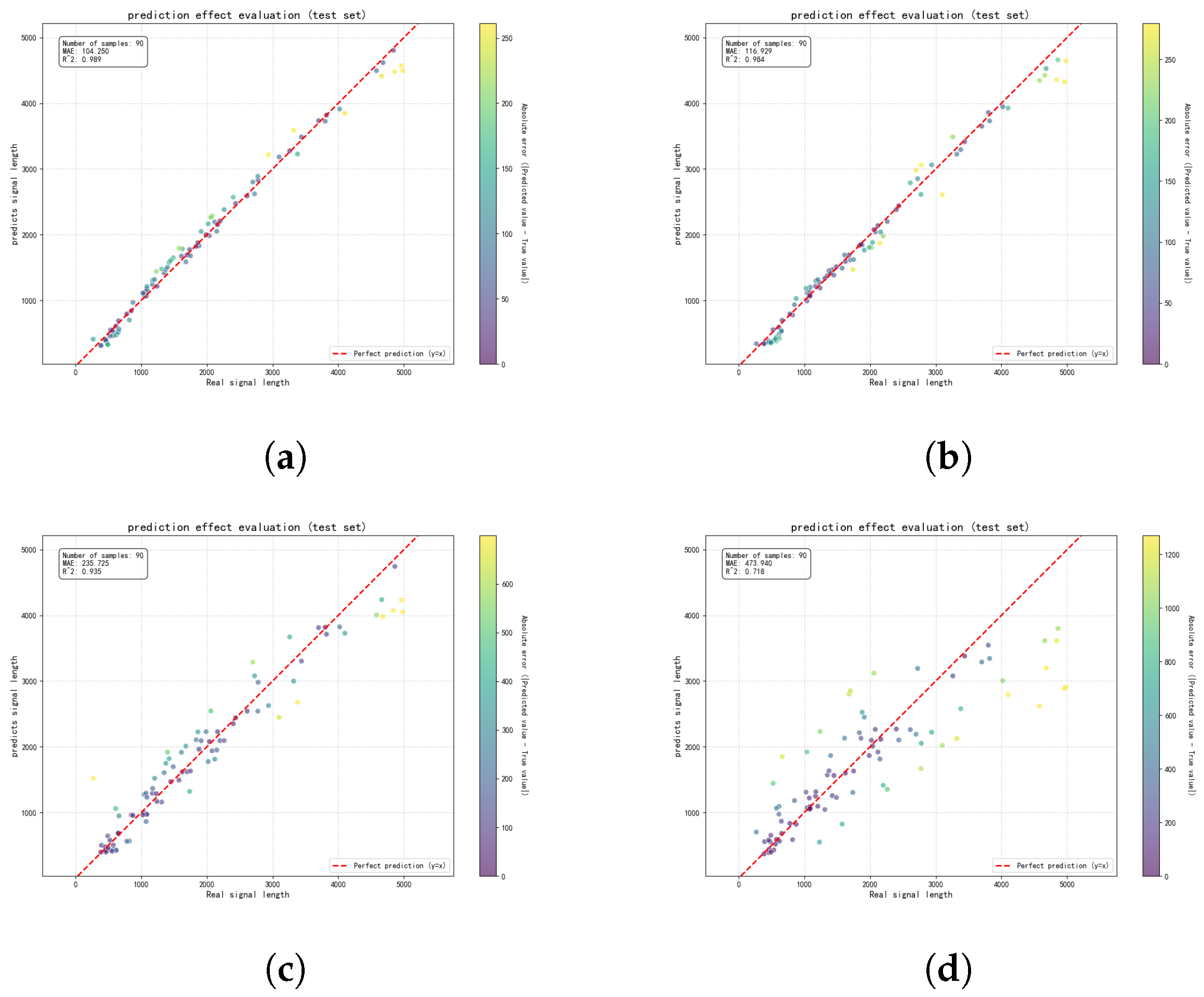
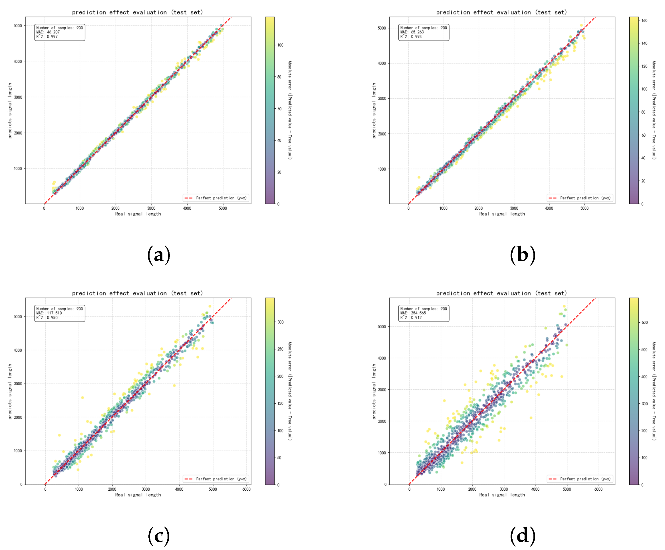
5.1.4. ISRJ Parameter Estimation Results

To compare the impact of feature fusion on the parameter estimation task, this paper estimates the ISRJ-sampling duration using the same convolutional neural network, both with and without feature fusion. The dataset comprises 6000 spectrograms, for which the sampling duration ranges from 500 to 5000 (in units of 0.01 $\mathsf{\mu }\mathrm{s}$). These spectrograms were divided into training, validation, and test sets at a ratio of 0.7:0.15:0.15. Figure 23 shows the accuracy of the ISRJ-sampling duration estimation. In the figure, the red dashed line represents the ideal prediction curve (predicted value = true value). The color intensity of the scattered points indicates the magnitude of the absolute error, where darker colors represent larger absolute errors.

Figure 23a shows the sampling-duration estimation results relying solely on spectrogram features. As observed from the scatter plot distribution, although most prediction points are clustered near the ideal prediction curve, the error increases notably when the signal’s sampling duration is long, and some scatter points deviate significantly from the actual results.The mean absolute error is relatively high (approximately 1.35 $\mathsf{\mu }\mathrm{s}$). The model’s coefficient of determination is 0.958, indicating that while the model can explain approximately 95.8% of the data variability, there is still significant room for overall performance improvement.

Figure 23b shows the sampling-duration estimation results using the feature fusion strategy. Compared to Figure 23a, its scatter points are noticeably more densely clustered around the ideal prediction curve, and there are no predictions that completely deviate from the true values. The mean absolute error is significantly reduced (approximately 0.47 $\mathsf{\mu }\mathrm{s}$). The coefficient of determination reaches 0.997, which is very close to 1, indicating a very high degree of fit between the model’s predicted values and the true values.

From the results in Figure 23, it can be concluded that adopting the feature fusion strategy can significantly improve the accuracy and robustness of ISRJ-sampling-duration estimation. Specifically, the estimations obtained using the feature fusion strategy show better consistency with the true values and smaller errors.

Furthermore, to analyze the accuracy of the proposed hybrid network for ISRJ sampling duration estimation under varying data volumes and SJRs, we set the dataset sizes to 600 and 6000 spectrograms, respectively. Parameter estimation was then performed on mixed signals at different SJRs using the proposed processing flow.

Figure 24 illustrates the ISRJ-sampling-duration-estimation performance using a dataset of 600 spectrograms across SJRs ranging from −1 dB to −10 dB (Figure 24a–d). With this smaller dataset, the model achieved good estimation results at an SJR of −1 dB. The performance remained high at −5 dB, with only a slight increase in MAE (from ≈1.04 $\mathsf{\mu }\mathrm{s}$ to ≈1.16 $\mathsf{\mu }\mathrm{s}$) and nearly unchanged $R^2$. Even at an SJR of −8 dB, the estimation error was acceptable (MAE ≈ 2.35 $\mathsf{\mu }\mathrm{s}$). However, at an SJR of −10 dB, the MAE increased significantly, and the $R^2$ dropped to 0.718, indicating a substantial decline in model accuracy and reliability.

In contrast, Figure 25 presents the results using a larger dataset of 6000 spectrograms under the same SJR conditions. Compared to the 600-spectrogram case, this larger dataset markedly improved performance, especially at low SJRs. Notably, even at an SJR of −10 dB, the model achieved an $R^2$ of 0.912, demonstrating a significantly higher accuracy and reliability.

The computational efficiency of our framework is rooted in its design. The front-end signal separation simplifies the task, allowing the subsequent HMFN to be highly specialized. Furthermore, the HMFN’s complexity is minimized by the adaptive time–frequency map cropping, which constrains the CNN’s input to an information-rich 148 × 100 region. As a result, the HMFN is a lightweight model containing only 0.13 M parameters and requiring 0.15 GFLOPs for inference. These metrics underscore the model’s low computational footprint and affirm its suitability for real-time radar signal processing.

6. Results

This study tackles the precise estimation of the ISRJ-sampling duration in complex electromagnetic environments where suppressive and deceptive jamming coexist. We proposed and validated an approach combining the FRFT with a Hybrid Modality Fusion Network. The FRFT, augmented by adaptive time–frequency masking, effectively separated ISRJ and target echo from the mixed signal, even under strong interference. Subsequently, the HMFN, which integrates deep visual features from spectrograms with handcrafted features derived from underlying mechanisms, achieved high-precision estimation of the ISRJ-sampling duration.

Numerical simulations demonstrated the robustness and effectiveness of our proposed methodology. Notably, when trained and validated on a comprehensive dataset of 6000 spectrograms, the HMFN demonstrated significant robustness, yielding a coefficient of determination ($R^2$) of 0.912 for ISRJ-sampling-duration estimation even at a suppressive SJR of −10 dB. This high level of accuracy under severe interference conditions underscores the method’s potential for providing crucial parameter support for active electromagnetic countermeasures and enhancing the radar’s cognitive anti-jamming capabilities.

The proposed framework is tailored for operational scenarios characterized by the coexistence of suppressive noise and LFM-based deceptive jammers, such as ISRJ and SMSP jamming. This approach leverages the inherent ability of the FRFT to achieve a high energy concentration for chirp signals. Consequently, a primary limitation is the expected performance degradation when encountering non-LFM jamming waveforms. Future research will focus on extending the framework’s scope to more complex jamming scenarios while deepening its analytical capabilities. This includes addressing a wider range of deceptive and suppressive techniques, such as velocity deception and advanced composite jamming. In parallel, the HMFN will be enhanced to perform multi-parameter estimation for ISRJ signals, identifying key attributes, like forwarding count, sampling period, number of samples, and forwarding delay. Such advancements will enable a more granular characterization of the threat environment, strengthening the system’s practical value for intelligent electronic countermeasures.

References

1. Chen, X.; Liu, Y.; Wang, C. Multi-Domain Fusion Network for Active Jamming Recognition in Cognitive Radar. Remote Sens. 2025, 17, 1723. [Google Scholar] [CrossRef]
2. Zhou, H.; Wang, L.; Guo, Z. A Radar Compound Jamming Recognition Method Based on Blind Source Separation. IEEE Trans. Aerosp. Electron. Syst. 2024, 60, 9073–9084. [Google Scholar] [CrossRef]
3. Pan, Y.; Xie, D.; Zhao, Y.; Wang, X.; Huang, Z. Overview of Radar Jamming Waveform Design. Remote Sens. 2025, 17, 1218. [Google Scholar] [CrossRef]
4. Han, R.; Li, X.; Xu, X.; Zhang, Z.; Zhang, T. Adaptive Reconnaissance and Suppressive Jamming Strategy Generation Based on Reinforcement Learning. IEEE Trans. Aerosp. Electron. Syst. 2025, early access. [Google Scholar] [CrossRef]
5. Li, Q.; Guo, Y.; Zhang, P.; Xu, H.; Zhang, L.; Chen, Z.; Huang, Y. Deception Velocity-Based Method to Discriminate Physical Targets and Active False Targets in a Multistatic Radar System. Remote Sens. 2024, 16, 382. [Google Scholar] [CrossRef]
6. Orduyilmaz, A.; Ispir, M.; Serin, M.; Efe, M. Ultra wideband spectrum sensing for cognitive electronic warfare applications. In Proceedings of the 2019 IEEE Radar Conference (RadarConf), Boston, MA, USA, 22–26 April 2019. [Google Scholar]
7. Lei, Z.; Qu, Q.; Chen, H.; Zhang, Z.; Dou, G.; Wang, Y. Mainlobe Jamming Suppression With Space-Time Multichannel via Blind Source Separation. IEEE Sens. J. 2023, 23, 17042–17053. [Google Scholar] [CrossRef]
8. Lv, Q.; Liu, L.; Wu, Y.; Peng, M.; Quan, Y. A Framework for Compound Interrupted Sampling Repeater Jamming Parameter Measurement. IEEE Trans. Instrum. Meas. 2025, 74, 2507704. [Google Scholar] [CrossRef]
9. Liu, Q.; Sui, X.; Chen, X.; Liang, Z.; Zhu, R. Jamming suppression by blind source separation: From a perspective of spatial band-pass filters. J. Syst. Eng. Electron. 2025, 1–8. [Google Scholar] [CrossRef]
10. Luo, W.; Jin, H.; Li, H.; Duan, K. Radar Main-Lobe Jamming Suppression Based on Adaptive Opposite Fireworks Algorithm. IEEE Open J. Antennas Propag. 2021, 2, 138–150. [Google Scholar] [CrossRef]
11. Lu, L.; Gao, M. A Truncated Matched Filter Method for Interrupted Sampling Repeater Jamming Suppression Based on Jamming Reconstruction. Remote Sens. 2022, 14, 97. [Google Scholar] [CrossRef]
12. Lu, L.; Gao, M. An Improved Sliding Matched Filter Method for Interrupted Sampling Repeater Jamming Suppression Based on Jamming Reconstruction. IEEE Sens. J. 2022, 22, 9675–9684. [Google Scholar] [CrossRef]
13. Dai, H.; Zhao, Y.; Su, H.; Wang, Z.; Bao, Q.; Pan, J. Research on an Intra-Pulse Orthogonal Waveform and Methods Resisting Interrupted-Sampling Repeater Jamming within the Same Frequency Band. Remote Sens. 2023, 15, 3673. [Google Scholar] [CrossRef]
14. Chao, Z.; Liu, Q.; Tao, Z. Research on DRFM Repeater Jamming Recognition. J. Signal Process. 2017, 33, 911–917. [Google Scholar] [CrossRef]
15. Liu, M.; Chen, J.; Pan, X.; Zhao, F. Parameter Estimation for Interrupted-Sampling Jamming Recognition Based on Piecewise Shannon Entropy. In Proceedings of the 2022 International Applied Computational Electromagnetics Society Symposium (ACES-China), Xuzhou, China, 9–12 December 2022. [Google Scholar]
16. Liu, L.; Lv, Q.; Liu, J.; Wu, Y.; Quan, Y. Adaptive Parameter Estimation for Compound Interrupted Sampling and Repeating Jamming. IEEE Signal Process. Lett. 2024, 31, 496–500. [Google Scholar] [CrossRef]
17. Wang, X.; Li, B.; Chen, H.; Liu, W.; Zhu, Y.; Luo, J.; Ni, L. Interrupted-Sampling Repeater Jamming Countermeasure Based on Intrapulse Frequency–Coded Joint Frequency Modulation Slope Agile Waveform. Remote Sens. 2024, 16, 2810. [Google Scholar] [CrossRef]
18. Han, B.; Qu, X.; Yang, X.; Li, W.; Zhang, Z. DRFM-Based Repeater Jamming Reconstruction and Cancellation Method with Accurate Edge Detection. Remote Sens. 2023, 15, 1759. [Google Scholar] [CrossRef]
19. Zhe, Z. Radar Signal Recognition and Parameter Estimation Based on FRFT. Master’s Thesis, Harbin Engineering University, Harbin, China, 2020. [Google Scholar]
20. Wen, Z.; Liu, M.; Chen, Y.; Zhao, N.; Nallanathan, A.; Yang, X. Multi-Component LFM Signal Parameter Estimation for Symbiotic Chirp-UWB Radio Systems. IEEE Trans. Cogn. Commun. Netw. 2024, 10, 1608–1619. [Google Scholar] [CrossRef]
21. Deng, J.; Sun, Z.; Li, X.; Cui, G. ASC-BSS-Based Parameter Estimation Method for Multiple LFM Pulses With Aliasing Effect From Passive Radar. IEEE Trans. Aerosp. Electron. Syst. 2025, 61, 5132–5144. [Google Scholar] [CrossRef]
22. Wang, P.; Yang, J.; Du, Y. A fast algorithm for parameter estimation of multi-component LFM signal at low SNR. In Proceedings of the 2005 International Conference on Communications, Circuits and Systems, Hong Kong, China, 27–30 May 2005; Volume 2, pp. 765–768. [Google Scholar]
23. Gong, S.; Wei, X.; Li, X. ECCM scheme against interrupted sampling repeater jammer based on time-frequency analysis. J. Syst. Eng. Electron. 2014, 25, 996–1003. [Google Scholar] [CrossRef]
24. Ji, H. Parameter Estimation of LFM Signal Based on Radon-WDL Transform and Its Application. Master’s Thesis, University of Electronic Science and Technology of China, Chengdu, China, 2017. [Google Scholar]
25. Tingyu, N. Research on Parameter Estimation Algorithm of LPI Radar Signals Based on T-F Analysis. Master’s Thesis, Xidian University, Xi’an, China, 2017. [Google Scholar]
26. Xie, Q.; Wang, Z.; Wen, F.; He, J.; Truong, T.K. Coarray Tensor Train Decomposition for Bistatic MIMO Radar with Uniform Planar Array. IEEE Trans. Antennas Propag. 2025, early access. [Google Scholar] [CrossRef]
27. Hao, L. Research on Radar Jamming Suppression Based on Jamming Cognition. Master’s Thesis, University of Electronic Science and Technology of China, Chengdu, China, 2021. [Google Scholar]
28. Duong, V.M.; Vesely, J.; Hubacek, P.; Janu, P.; Tran, X.L. Detection and parameter estimation of intra-pulse modulated radar signals in complex interference environments+. SN Appl. Sci. 2023, 5, 184. [Google Scholar] [CrossRef]
29. Shi, Z.; Wu, H.; Zhu, X.; Wang, W.; Ni, X.; Zhang, J. Interrupted sampling forwarding jamming parameter estimation based on YOLOv7-tiny. In Proceedings of the 2024 IEEE 7th International Conference on Electronic Information and Communication Technology (ICEICT), Xi’an, China, 31 July–2 August 2024; pp. 144–149. [Google Scholar]
30. Meng, Y.; Yu, L.; Wei, Y. Multiple information cognition of interrupted sampling repeater jamming in complex scenes. In Proceedings of the 2021 CIE International Conference on Radar (Radar), Haikou, China, 15–19 December 2021; pp. 2176–2179. [Google Scholar]
31. He, X.; Liao, K.; Peng, S.; Tian, Z.; Huang, J. Interrupted-Sampling Repeater Jamming-Suppression Method Based on a Multi-Stages Multi-Domains Joint Anti-Jamming Depth Network. Remote Sens. 2022, 14, 3445. [Google Scholar] [CrossRef]
32. Chao, Z.; Liu, Q.; Cheng, H. Time-frequency Analysis Techniques for Recognition and Suppression of Interrupted Sampling Repeater Jamming. J. Radars 2019, 8, 100–106. [Google Scholar]
33. Li, Y. Research on the Identification and Inhibition of SMSP and C&I Distance False Target Spoof Interference. Master’s Thesis, University of Electronic Science and Technology of China, Chengdu, China, 2012. [Google Scholar]
34. Wang, Y.; Liu, G.; Ma, X.; Song, C.; Jin, G.; Li, L. A Convolution Modulation Jamming Method Based on the Optimal Combination of Noise Templates. IEEE Geosci. Remote Sens. Lett. 2024, 21, 4008905. [Google Scholar] [CrossRef]
35. Li, T.; Zhang, J.; Lu, X.; Zhang, Y. SDBD: A Hierarchical Region-of-Interest Detection Approach in Large-Scale Remote Sensing Image. IEEE Geosci. Remote Sens. Lett. 2017, 14, 699–703. [Google Scholar] [CrossRef]
36. Chen, R.; Wang, Y. Universal FRFT-based algorithm for parameter estimation of chirp signals. J. Syst. Eng. Electron. 2012, 23, 495–501. [Google Scholar] [CrossRef]
37. Wei, S.D.; Lai, S.H. Fast Template Matching Based on Normalized Cross Correlation with Adaptive Multilevel Winner Update. IEEE Trans. Image Process. 2008, 17, 2227–2235. [Google Scholar] [CrossRef]
38. Liu, P.; Huang, W.; Zhang, W.; Li, F. An EMD-SG Algorithm for Spectral Noise Reduction of FBG-FP Static Strain Sensor. IEEE Photonics Technol. Lett. 2017, 29, 814–817. [Google Scholar] [CrossRef]
39. Chen, H.; Maharatna, K. An Automatic R and T Peak Detection Method Based on the Combination of Hierarchical Clustering and Discrete Wavelet Transform. IEEE J. Biomed. Health Inform. 2020, 24, 2825–2832. [Google Scholar] [CrossRef] [PubMed]
40. Lu, J.; Ma, C.X.; Zhou, Y.R.; Luo, M.X.; Zhang, K.B. Multi-Feature Fusion for Enhancing Image Similarity Learning. IEEE Access 2019, 7, 167547–167556. [Google Scholar] [CrossRef]
41. Zhang, C.; Liu, Y.; Si, W. PRI modulation recognition and sequence search under small sample prerequisite. J. Syst. Eng. Electron. 2023, 34, 706–713. [Google Scholar] [CrossRef]
42. Huang, J.; Chen, B.; Yao, B.; He, W. ECG Arrhythmia Classification Using STFT-Based Spectrogram and Convolutional Neural Network. IEEE Access 2019, 7, 92871–92880. [Google Scholar] [CrossRef]
43. Fagbohungbe, O.; Qian, L. The Effect of Batch Normalization on Noise Resistant Property of Deep Learning Models. IEEE Access 2022, 10, 127728–127741. [Google Scholar] [CrossRef]
44. Zhang, Z.; Xu, Z.Q.J. Implicit Regularization of Dropout. IEEE Trans. Pattern Anal. Mach. Intell. 2024, 46, 4206–4217. [Google Scholar] [CrossRef]
Figure 1. Transmitted LFM signal: (a) time-domain waveform; (b) TFR.
Remotesensing 17 02648 g001
Figure 2. ISDRJ signal: (a) time-domain waveform; (b) TFR.
Remotesensing 17 02648 g002
Figure 3. ISPRJ signal ( M = 3 ): (a) time-domain waveform; (b) TFR.
Remotesensing 17 02648 g003
Figure 4. ISCRJ signal: (a) time-domain waveform; (b) TFR.
Remotesensing 17 02648 g004
Figure 5. SMSP jamming (five sub-waveforms) with distinct frequency modulation: (a) time-domain waveform; (b) TFR.
Remotesensing 17 02648 g005
Figure 6. NCJ signal: (a) TFR of s j ( t ) showing its noise-like spread in time and frequency; (b) matched filter output forming a high-power, spread noise background.
Remotesensing 17 02648 g006
Figure 7. Proposed three-stage framework for the separation of ISRJ signals and target echo.
Remotesensing 17 02648 g007
Figure 8. Generation of the mixed signal in a battlefield environment, showing the synthesis of deception and suppression jamming by an adversary and their mixture with target echo and noise.
Remotesensing 17 02648 g008
Figure 9. TFR of mixed signal: (a) Target echo with ISRJ and SMSP jamming. (b) The same signal mixture with additional NCJ suppression jamming, causing severe masking.
Remotesensing 17 02648 g009
Figure 10. Radar-signal-processing results under mixed jamming conditions: (a) R-D map of the mixed signal, revealing numerous false peaks induced by jamming. (b) Outcome of CFAR detection on the R-D map from (a), where jamming-induced false targets are erroneously confirmed.
Remotesensing 17 02648 g010
Figure 11. FRFT-domain energy distribution of a mixed signal (SMSP jamming, ISRJ, target echo) versus transform order, showing distinct energy focusing for LFM components.
Remotesensing 17 02648 g011
Figure 12. Flowchart of the ISRJ (or target echoes) separation method.
Remotesensing 17 02648 g012
Figure 13. Adaptive time–frequency map cropping flowchart for efficient ISRJ signal component extraction.
Remotesensing 17 02648 g013
Figure 14. Overall architecture of the proposed HMFN for ISRJ-signal-sampling duration estimation.
Remotesensing 17 02648 g014
Figure 15. Fractional Fourier Transform (FRFT) results for SMSP-jamming chirp rate estimation, performed at optimal orders corresponding to assumed multiplication factors of its chirp rate relative to the echo signal: (a) Factor = 4; (b) Factor = 5 (showing clear energy focusing for SMSP jamming); (c) Factor = 6.
Remotesensing 17 02648 g015
Figure 16. TFR of the mixed signal after SMSP-jamming suppression via FRFT-domain masking.
Remotesensing 17 02648 g016
Figure 17. Optimal-order FRFT of the mixed signal, showing sharp energy peaks for the target echo and ISRJ.
Remotesensing 17 02648 g017
Figure 18. TFRs of separated signal: (a) target echo; (b) ISRJ signal.
Remotesensing 17 02648 g018
Figure 19. TFRs of the separated signal under different SNR conditions: (a) SNR = 5 dB (b) SNR = 0 dB (c) SNR = −5 dB.
Remotesensing 17 02648 g019
Figure 20. TFRs of separated ISRJ components for different jamming types: (a) ISDRJ (b) ISPRJ (c) ISCRJ.
Remotesensing 17 02648 g020
Figure 21. Peak cluster center detection results for three ISRJ subtypes, facilitating main component localization for efficient spectrogram cropping: (a) ISDRJ; (b) ISPRJ; (c) ISCRJ.
Remotesensing 17 02648 g021
Figure 22. Cropped spectrograms of different ISRJ subtypes, serving as efficient inputs for neural network processing (dimensions reduced, from 512 × 184 to 148 × 100): (a) ISDRJ; (b) ISPRJ; (c) ISCRJ.
Remotesensing 17 02648 g022
Figure 23. Impact of feature fusion on ISRJ-sampling-duration-estimation accuracy using the test set. Scatter plots show predicted versus true values (durations in 0.01 μ s units; color indicates absolute error): (a) Spectrogram features only (MAE ≈ 1.35 μ s , R 2 = 0.958); (b) With feature fusion, showing improved accuracy (MAE ≈ 0.47 μ s , R 2 = 0.997).
Remotesensing 17 02648 g023
Figure 24. ISRJ-sampling-duration-estimation performance versus SJR using a dataset of 600 spectrograms (durations in 0.01 μ s units; color indicates absolute error): (a) SJR = −1 dB (MAE ≈ 1.04 μ s , R 2 = 0.989); (b) SJR = −5 dB (MAE ≈ 1.16 μ s , R 2 = 0.984); (c) SJR = −8 dB (MAE ≈ 2.36 μ s , R 2 = 0.935); (d) SJR = −10 dB (MAE ≈ 4.74 μ s , R 2 = 0.718).
Remotesensing 17 02648 g024
Figure 25. ISRJ-sampling-duration-estimation performance versus SJR using a dataset of 6000 spectrograms (durations in 0.01 μ s units; color indicates absolute error): (a) SJR = −1 dB (MAE ≈ 0.21 μ s , R 2 = 0.997); (b) SJR = −5 dB (MAE ≈ 0.36 μ s , R 2 = 0.992); (c) SJR = −8 dB (MAE ≈ 0.61 μ s , R 2 = 0.982); (d) SJR = −10 dB (MAE ≈ 0.91 μ s , R 2 = 0.912).
Remotesensing 17 02648 g025