SDDGRNets: Level–Level Semantically Decomposed Dynamic Graph Reasoning Network for Remote Sensing Semantic Change Detection

Abstract

Semantic change detection technology based on remote sensing data holds significant importance for urban and rural planning decisions and the monitoring of ground objects. However, simple convolutional networks are limited by the receptive field, cannot fully capture detailed semantic information, and cannot effectively perceive subtle changes and constrain edge information. Therefore, a dynamic graph reasoning network with layer-by-layer semantic decomposition for semantic change detection in remote sensing data is developed in response to these limitations. This network aims to understand and perceive subtle changes in the semantic content of remote sensing data from the image pixel level. On the one hand, low-level semantic information and cross-scale spatial local feature details are obtained by dividing subspaces and decomposing convolutional layers with significant kernel expansion. Semantic selection aggregation is used to enhance the characterization of global and contextual semantics. Meanwhile, the initial multi-scale local spatial semantics are screened and re-aggregated to improve the characterization of significant features. On the other hand, at the encoding stage, the weight-sharing approach is employed to align the positions of ground objects in the change area and generate more comprehensive encoding information. Meanwhile, the dynamic graph reasoning module is used to decode the encoded semantics layer by layer to investigate the hidden associations between pixels in the neighborhood. In addition, the edge constraint module is used to constrain boundary pixels and reduce semantic ambiguity. The weighted loss function supervises and optimizes each module separately to enable the network to acquire the optimal feature representation. Finally, experimental results on three open-source datasets, such as SECOND, HIUSD, and Landsat-SCD, show that the proposed method achieves good performance, with an SCD score reaching 35.65%, 98.33%, and 67.29%, respectively.

1. Introduction

As one of the basic tasks of change detection [1], semantic change detection [2] mainly involves identifying the process of change among remote sensing data in the area of interest at different times, exploring the process of regional changes in multi-temporal remote sensing data that are co-registered with geographic information. Improvements in image resolution and morphological diversity have allowed researchers to understand these changes more precisely, better capturing spatial features, achieving higher semantic accuracy on remote sensing data, and providing reliable technical support for subsequent applications. The semantic change detection of remote sensing data is used in multiple fields; for example, in agricultural surveys [3], deforestation monitoring [4], disaster loss assessment [5], and ecosystem monitoring [6]. However, a simple semantic change detection scheme cannot fully catch these subtle changes in multi-temporal data [7], resulting in poor detection performance. Therefore, with the effective implementation of deep feature extraction techniques across various fields, observing remote sensing data at multiple temporal stages within the same region has become a hot topic in semantic detection to assist experts in urban and rural planning.

Early change detection methods focused on handwork feature design and screening. They used simple machine learning methods [8], such as statistics and linear transformation [9], to distinguish alterations in images of the same region at different phases. These methods are expensive, and their manual features are heavily dependent on expert experience; that is, the quality of the features directly influences the accuracy of remote sensing image change detection. Change detection methods using deep learning technology [1,10] use the powerful self-learning capability of neurons and change the activation state of neurons to perform intrinsic semantic modeling on remote sensing data at various temporal stages, which can effectively solve the errors caused by manual features and reduce data annotation costs. Change detection accuracy has also significantly improved. Some existing end-to-end detection methods using simple convolutional neural networks [11] and a transformer [12,13] enhance the accuracy of semantic change detection by encoding and decoding remote sensing data as semantic segmentation and “change–no change” in different time periods. Although these methods improve the detection performance, they do not address practical constraints at the detection stage, resulting in significant differences in spatial features obtained during multiple phases and in the same region, and ignoring these differences and the semantic association between remote sensing data from different phases in the feature fusion stage. Many researchers have designed a multi-branch semantic learning network [14,15] to ensure the alignment of features in changing areas of remote sensing data across multiple periods. This network effectively perceives the changes in the target object’s position in the remote sensing image under semantic segmentation. Although these methods achieved a good constraint and detection performance, they entirely ignore the fact that weight-sharing between features on different branches benefits semantic change detection. Meanwhile, the entanglement of intermediate features in the feature extraction stage leads to a further decline in model performance. In the feature fusion stage, a simple splicing method is used, which is unable to represent significant features and strengthens the propagation of superfluous semantic information across layers. Therefore, the effectiveness of semantic change detection still has much room for improvement.

To solve these problems, we developed an semantically decomposed dynamic graph reasoning network (SDDGRNets) for multi-temporal remote sensing semantic change detection, which aims to explore semantic associations among feature maps of different scales and generate effective pixel-level semantic change maps at each stage. The framework models remote sensing data from different time points through two identical encoding branches and generates multi-scale encoded semantics. It highlights the differences between changed and unchanged categories at different scales and strengthens the correlation between similar targets. Secondly, a newly designed semantic dynamic graph reasoning module decodes this encoded information. Through the dynamic aggregation and transmission functions of graph reasoning nodes, the differences between different types of targets on remote sensing data are strengthened and feature alignment between decoded semantics is achieved. In addition, remote sensing data at different times from weight-sharing in the encoding stage are used to reduce entanglement between intermediate features. Meanwhile, the newly designed semantic screening module refines the generated semantic graph from coarse to fine stages. It provides deep constraints on semantic graphs of different phases and scales. These deep constraints can effectively improve pixel semantics’ representation at the target’s edge.

The contributions are as follows:

• A dynamic graph reasoning network (SDDGRNets) is developed via layer–layer semantic decomposition for semantic change detection in remote sensing data. It seeks to achieve the encoding and decoding of target semantic information in remote sensing data through an end-to-end approach and obtain more effective multi-scale spatiotemporal semantic details. Semantic information from the same area is constrained and aligned through encoding weight-sharing and layer-by-layer semantic decomposition, and semantic interaction is constructed using remote sensing data from various temporal stages to meet the accuracy requirements of semantic change detection.
• A dynamic graph reasoning module is developed to reduce the semantic ambiguity of edge pixels from the same types of targets in remote sensing data and highlight the differences between pixels from different types of targets. The dynamic fusion capability of graph reasoning nodes is used to perceive the subtle changes in targets in the same area in multi-temporal remote sensing data, and further strengthens the interaction and association between corresponding pixels. In addition, a combination of main and multiple auxiliary losses is used to perform strong supervision training on each module to enable the network to attain a superior performance. Meanwhile, edge pixels located in changed and unchanged areas are penalized and constrained, and class weights are used to balance target objects of different sizes in the image. Finally, the proposed method is evaluated on multiple remote sensing image semantic change detection datasets, proving that it outperforms other advanced methods.

Other organizations involved in this study are as follows: Section 2 focuses on related works on semantic change detection. Section 3 elaborates on the proposed SDDGRNets method for semantic change detection in remote sensing data, focusing on the internal modules’ working principle and structure. Section 4 presents the experimental results and discussion, and provides visualizations. Section 5 presents the conclusions and future research plans.

2. Related Works

Early change detection mainly relied on manual features made using expert experience, and these features were passed to simple classifiers to determine between changed and unchanged categories. For example, Zerrouki N et al. [16] proposed combining the Hotelling T2 control method and the weighted random forest classifier to identify land cover changes. They verified and evaluated the method on the SZTAKI AirChange dataset. To improve the monitoring of environmental changes, Goswami A et al. [17] designed two change detection methods: a separability matrix and image difference decision tree. The former mainly classifies and compares the feature matrix generated by the decision tree, and the latter distinguishes between changed–unchanged pixels by calculating the threshold of the changed images by applying the corner point method. To observe the real-time interaction between scene data and spatial environment data, Wang J et al. [18] adopted a variety of strategies, such as change occurrence description, transformation, diffusion, and the spatiotemporal transformation mechanism of spatial patterns, to identify land utilization and surface cover alterations. To evaluate the changes in land utilization patterns caused by coal mining from 2006 to 2016, Karan S K et al. [19] proposed a method combining the support vector machine and maximum likelihood methods. They used support vector machine to classify multi-temporal remote sensing data and the maximum likelihood method to compare different classification outcomes to derive the final land change situation. Although these change detection methods, based on hand-crafted features, assist experts in judging regional changes in remote sensing data, they require experts to participate in feature engineering and selection and rely heavily on experts’ experience, making it difficult for them to satisfy the expanding practical requirements. Furthermore, they are time-consuming, labor-intensive, and costly, with limited detection precision and weak generalizability.

Deep learning has rapidly developed in the change detection field [3,4,5]. Many researchers have used deep learning technology to develop automated systems to achieve semantic change detection in multi-temporal remote sensing data, and provide reliable information for experts in domains including urban and rural planning and ecosystem monitoring. For example, He H et al. [20] considered that land change information provides an essential theoretical basis for urban and rural management and designed a semantic change detection method based on a deep learning network, which alleviates the semantic variations between images of different time series by obtaining the spatial, time, and content information of the changed area in the image. To achieve semantic change detection, Papadomanolaki M et al. [21] proposed a UNet-like architecture, which uses integrated, fully convolutional LSTM blocks at each level to observe the chronological correlation of spatial feature representations, so that the framework can combine segmentation and change detection using a fully convolutional long short-term memory (LSTM) network. Lei Y et al. [22] proposed a hierarchical paired channel fusion network (HPCFNet) to detect street scene changes. The intuitive method integrates the derived image feature pairs and directly assess the differences to generate a map of changes. The network uses the adaptive fusion of paired feature channels to locate and identify the changes between image pairs. Additionally, considering the observations of the diversity of scene change distribution, a multi-part feature learning (MPFL) strategy is adopted in the model to detect diverse changes. To overcome the shortcomings of remote sensing image street scene semantic segmentation and the change detection dataset, Sakurada K et al. [23] proposed a novel, weakly supervised, semantic scene change detection scheme. On the one hand, this detects the change mask and estimates the pixel-level semantic labels separately. On the other hand, considering the differences in camera viewpoints, a novel dual network architecture with a correlation layer is introduced to achieve accurate semantic change detection in remote sensing data. You et al. [24] developed an edge-guided remote sensing image change detection method to improve the edge representation ability and detection accuracy of targets in remote sensing data. This method first uses a dual-branch network structure to extract the regional spatial features and edge information of remote sensing image pairs of different time series. Secondly, a separate feature fusion module is used to aggregate the regional features and edge information of remote sensing data of different time series. Meanwhile, an edge-enhanced upsampling strategy is employed at the decoding stage to reconstruct the edge region features, further ensuring the accuracy of the edge information. Li M et al. [25] developed a semantic stream edge perception approach for remote sensing image change detection tasks. This method first utilizes pyramid features to enhance semantic information at various scales and embeds components that facilitate the transmission of semantic information flow, enabling the network to obtain optimal semantics and maximize the representation of key information. Meanwhile, the edge features of changing areas in the remote sensing data are refined through the edge perception component.Although these methods diminish the errors resulting from handcrafted feature engineering and selection, most of them use a single-scale network structure. Because of the constraints of the receptive field, it is challenging to obtain multi-scale information and high-level discriminative features of the change areas in remote sensing image pairs. Additionally, they often use semantic segmentation and change detection in series to achieve the final semantic change detection task, which causes error accumulation, is too complicated, and is unsuitable for large-scale remote sensing image pairs.

To promote the annotation efficiency of remote sensing image pairs and reduce the propagation of errors, pixel-level annotation methods are widely used in semantic change detection tasks combined with multi-tasks, and semantic segmentation and change detection tasks are realized simultaneously. For example, Ding L et al. [26] proposed a semantic change detection method using a multi-branch convolutional neural network that captures fine-grained semantic change information to better observe land cover/land use categories. The semantic temporal features are integrated into a deep change detection unit, and correlation is established between the remote sensing data of different time series, ensuring semantic consistency between them. Wang Q et al. [27] considered that traditional semantic change detection methods heavily rely on high consistency in the bi-temporal feature space when modeling difference features, resulting in false positives or negatives in the change area. Therefore, a semantic change detection framework of a cross-difference semantic consistency network is proposed, aiming to mine the variations in the bi-temporal instance features and preserve their semantic coherence. Additionally, to enhance the distinguishing capabilities of the model in the change area, the semantic co-alignment (SCA) loss function is introduced in combination with the principle of contrastive learning to further improve the intra-class consistency and inter-class distinction of the bi-temporal semantic features. Mei L et al. [28] proposed a semantic change detection method combined with SAM, introduced a contextual semantic change-aware dual encoder, combined MobileSAM and CNN in the encoder, extracted progressive semantic change features in parallel, and injected local features into the MobileSAM encoder through deep feature interaction (DFI) to compensate for Transformer’s constraints in perceiving local semantic details. Tang et al. [29] designed a multi-task joint learning ClearSCD method to improve the dependency between semantic information and change regions, thereby establishing a mutual gain relationship between different semantics. The method utilizes the first module to extract semantic information from various time series images, while the second module acquires the association between semantic types and binary changes, and finally enhances the contrast learning module to improve the detection performance. As traditional change detection methods are often difficult to generalize across semantic categories in real scenarios, Zhu Y et al. [30] designed a new semantic change detection method, which primarily utilizes the CLIP component to extract local features from images across different time series, and employs open semantic prompts to enhance the final detection accuracy. Although these methods diminish the spread of accumulated errors and enhance the performance of semantic change detection, they do not consider the hierarchical semantic correlation between remote sensing data of different time series in the feature learning stage, ignore the hidden association between pixel pairs in the same region, and fail to fully utilize the semantic details of boundary pixels in the semantic segmentation state.

With the effective implementation of graph neural networks across various domains, many researchers have applied them to semantic change detection tasks, considering the transmission and aggregation functions of graph nodes. For example, Long J et al. [31] proposed a hierarchical semantic graph interaction network (HGINet) for semantic change detection in high-resolution remote sensing data to mine the correlation between remote sensing image pairs from various temporal sequences. This method constructs a multi-level perceptual fusion network with a pyramid architecture and distinguishes the semantic features of different categories at multiple levels. Furthermore, the temporal correlation module between different features is used to model the correlation between bi-temporal semantic features to enhance the recognition of unchanged areas, and the semantic difference interaction module of the graph convolutional network is used to measure the bi-temporal semantic features and the interaction established between the corresponding difference features. Shi A et al. [32] proposed a graph semantics-guided Transformer network (GGTNet), using the graph semantic features obtained by the graph convolutional neural network to guide the multi-layer CNN and Transformer layers and improve the representation of semantic features. Cui B et al. [33] considered that the current popular CD technology mainly focuses on extracting deep semantic features and pixel-level interactions, while ignoring the potential advantages of cluster-level semantic interactions in bi-temporal images. They proposed a bi-temporal graph semantic interaction network for remote sensing image change detection. They clustered the land cover types in the bi-temporal images using soft clustering for each pixel, and projected each cluster to the vertex in the graph space. Meanwhile, they introduced a graph semantic interaction module to strengthen the correlation between bi-temporal features at the semantic level and effectively improved the information coupling between bi-temporal features, thereby suppressing information irrelevant to the task. These graph neural network change detection methods are mostly focused on the "change–unchanged" task, and there are few semantic change detection tasks in multi-temporal remote sensing data. Moreover, they mainly use graph convolutional neural networks to cluster semantic information, without considering the semantic ambiguity of edge pixels between multi-category targets. Meanwhile, there is insufficient correlation between features of different scales, and they are committed to exploring the high-level features of the change area of remote sensing data, while ignoring the abundant semantic information embedded in the low-level features, which affects the accuracy of the final semantic change detection.

3. Methods

In this section, we focus on the basic working of the proposed SDDGRNets remote sensing data semantic change detection architecture (See Section 3.1). Then, we present the internal constituent modules (see Section 3.2, Section 3.3, Section 3.4, Section 3.5, Section 3.6) and detail the algorithm’s learning procedure and implementation.

3.1. Overview

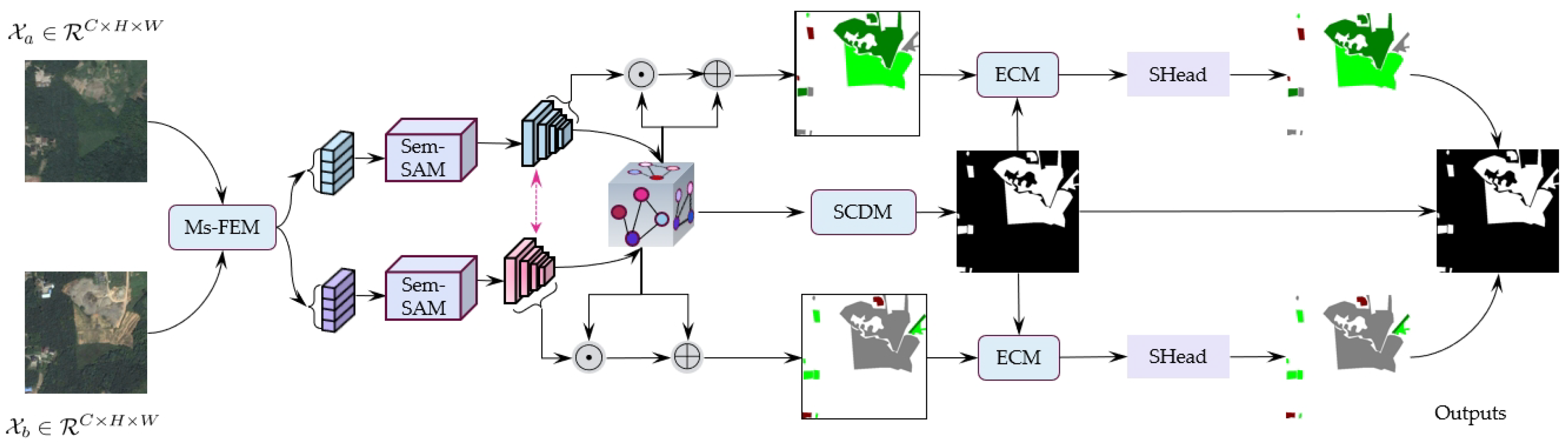
Figure 1 indicates the overall architecture of SDDGRNets for semantic change detection in remote sensing data. The method mainly consists of a unified multi-scale feature extraction module (Ms-FEM), a semantic selection aggregation module, an encoding–decoding module with a weight-sharing strategy, an edge constraint module (ECM), a semantic segmentation head (SHead), and a change detection module (SCDM). The multi-scale feature extraction module (Ms-FEM) mainly performs an initial semantic modeling on remote sensing data pairs ${\mathcal{X}}_a$ and ${\mathcal{X}}_b$ of different time, describes the target details within the region of alteration in remote sensing data from different scales, retains the fundamental attribute information, including the physical appearance of the target in the remote sensing data as much as possible while obtaining spatial semantics, and uses abundant low-level semantic details to enhance the model indicators and the model’s understanding of the remote sensing data content. The semantic selection aggregation module (Sem-SAM) aims to filter the initial multi-scale local spatial semantics and establish dependencies and interactions between different scales. Meanwhile, these filtered feature details are re-aggregated to form complementary relationships, reduce the redundant information between layers, and obtain frequency-hopping with more critical semantic information. For the encoding–decoding module with a weight-sharing strategy, a multi-semantic enhanced visual attention network (MSE-VAN) is used to encode the aggregated semantic information, and the weight-sharing approach is employed to perceive the deviation in the position of the target in the area of change between different temporal remote sensing image pairs to ensure consistency and alignment between features. Then, the dynamic graph reasoning module (DGRM) is used to upsample each encoded feature, reform layer-by-layer fusion decoding, form multi-scale decoding semantics, and generate corresponding semantic segmentation masks. To enable the network to obtain more effective edge information, the initial multi-scale spatial local details are feature-mapped and embedded into the segmentation and change detection mask, and the representation of target boundary pixels and edge information in the remote sensing image pair is further improved. Finally, semantic change detection is conducted using the segmentation and change detection heads. In addition, multiple loss functions are weighted to conduct an individual supervised training on each module, enabling the network to achieve optimal feature representation and detection performance. In summary, the proposed SDDGRNets remote sensing semantic change detection framework first inputs remote sensing image pairs of different time series into the multi-scale feature extraction module (Ms-FEM) to obtain multi-scale spatial semantic details of different targets in the image, and then passes these multi-scale features to the semantic aggregation module (Sem-SAM) to achieve weight-sharing and reduce the semantic differences between multi-scale characteristics. Meanwhile, associations and complementarities are established between different scales better to represent the objects within the remote sensing image pairs. Secondly, the dynamic graph reasoning module (DGRM) and boundary constraint module are utilized to enhance the information representation capabilities of edge pixels.

3.2. Initial Multi-Scale Feature Extraction Module (Ms-FEM)

Remote sensing data of different phases contain objects of different shapes and sizes in the changing area. They have significant differences in appearance and color. It is difficult for the feature information of a single structure to describe these contents. Multi-scale spatial local semantic features have proven beneficial for semantic segmentation and change detection tasks [34,35]. The receptive field limits the traditional single-scale convolution kernel, and it is challenging to acquire the semantic details of the target in the changing area of the remote sensing data pair. The subspace structure is divided to obtain a more effective semantic representation, and a set of dilated decomposition convolution layers is embedded to improve the ability to acquire semantic knowledge. The group attention is used to refine this semantic information along the channel to perceive the position changes among pixels within the region of alteration in the remote sensing image pair. Meanwhile, different dilated decomposition convolution kernels are used in parallel at the initial stage of feature semantics to enhance the low-level semantic characterization. The specific operation steps of the multi-scale feature extraction module (Ms-FEM) are as follows.

Step 1: A pair of remote sensing data of $\{{\mathcal{X}}_a,{\mathcal{X}}_b\}\in \mathcal{X}\in {\mathcal{R}}^{C\times H\times W}$, $C,H,W$ indicates the channel, height, and width dimensions of the input remote sensing image. These remote sensing image pairs are input into parallel dilated decomposition convolutional layers of different scales to extract the preliminary prior information of the target objects in the change area, which contains rich low-level semantic details of the target shape, size, and color. Prior knowledge ${\mathcal{F}}_0\left(\mathcal{X}\right)$ is presented in Equation (1):

$${\mathcal{F}}_0\left(\mathcal{X}\right)={\mathcal{H}}_{Max}\left[BN\left({\mathcal{H}}_{1\times 1}({\mathcal{H}}_{{\mathcal{K}}_1}^{\mathcal{DW}}\left(\mathcal{X}\right)\oplus {\mathcal{H}}_{{\mathcal{K}}_2}^{\mathcal{DW}}\left(\mathcal{X}\right)\oplus {\mathcal{H}}_{{\mathcal{K}}_3}^{\mathcal{DW}}\left(\mathcal{X}\right))\right)\right]$$

(1)

where ⊕ denotes feature concatenation; ${\mathcal{H}}_{{\mathcal{K}}_{1,2,3}}^{\mathcal{DW}}(·)$ denotes dilated decomposition convolution operations of different scales; ${\mathcal{K}}_{1,2,3}$ denotes convolution kernels of different sizes; ${\mathcal{H}}_{Max}[·]$ denotes the max pooling operation; ${\mathcal{H}}_{1\times 1}(·)$ denotes the ordinary convolution of $1\times 1$; $BN(·)$ denotes the batch normalization layer.

Step 2: ${\mathcal{F}}_0\left(\mathcal{X}\right)$ is input into the multi-level subspace feature extraction component using a residual strategy to represent and understand the ground objects in the changing area at the granular level [1,14]. Additionally, the extraction of local semantic details in multi-scale space is realized. The extraction of local spatial semantics at different scales is shown in Equation (2):

$${\mathcal{F}}_s\left(\mathcal{X}\right)={\Phi }_{rms}\left({\mathcal{F}}_0\left(\mathcal{X}\right)\right),s=\{1,2,3,4\}$$

(2)

where ${\Phi }_{rms}(·)$ represents the multi-level subspace feature extraction component of the residual strategy; $s=\{1,2,3,4\}$ represents this component’s different scales or feature extraction stages; ${\mathcal{F}}_0\left(\mathcal{X}\right)$ is first divided into $\pi$ feature maps $f_{\pi }\in {\mathcal{R}}^{{\displaystyle \frac{C}{\pi }}\times H\times W}$ of the same size along the channel for the subspace feature extraction component of the first level. Then, each feature map is input into a continuous $1\times 1$ convolution for feature compression and the elimination of redundant information, and a set of continuous $3\times 3$ size extended-convolution kernels undergo feature excitation to obtain more detailed local spatial features. The generated $\pi$ feature maps $f_{\pi }^{\prime }\in {\mathcal{R}}^{{\displaystyle \frac{C}{\pi }}\times H\times W}$ are weighted and fused using position attention [36,37] to enhance the perception of position and encoding capabilities among different channel features. Additionally, the component can be prompted to obtain more effective global contextual details in the channel dimension. Then, the new aggregation features are fed into the standard convolution layer and the batch normalization layer for further compression, and the initial semantic map with both position and channel-encoding information is obtained. The detailed semantic features ${\mathcal{F}}_1\left(\mathcal{X}\right)$ of the first level are shown in Equation (3):

$$\left\{\begin{array}{c}{f}_{\pi }^{\prime }={\mathcal{H}}_{1\times 1}^{\Delta }\left(f_{\pi }\right))\hfill \\ f_{\pi }^{″}={\mathcal{H}}_{3\times 3}^{\Delta ,D}\left(f_{\pi }^{\prime }\right)\hfill \\ f^{\prime }={\Phi }_{pam}[(f_1^{″}\oplus f_1^{\prime }),\cdots ,(f_c^{″}\oplus f_c^{\prime }),\dots ,(f_{\pi }^{″}\oplus f_{\pi }^{\prime })],1\le c\le \pi \le C\hfill \\ {\mathcal{F}}_1\left(\mathcal{X}\right)=BN\left({\mathcal{H}}_{1\times 1}\left(f^{\prime }\right)\right)\hfill \end{array}\right.$$

(3)

where ⊕ indicates feature concatenation; ${\Phi }_{pam}(·)$ indicates the position attention operation; ${\mathcal{H}}_{3\times 3}^{\Delta ,D}(·)$ indicates a set of continuous $3\times 3$ size extended-convolution operation; ${\mathcal{H}}_{1\times 1}^{\Delta }(·)$ indicates a set of continuous $1\times 1$ size convolution operation.

In summary, the multi-scale feature extraction module uses dilated convolution to increase the receptive field and obtain global contextual semantics of the ground objects in the change area. Furthermore, dividing the subspace along the channel and re-aggregating can obtain more effective local spatial detail features and reduce the transmission of redundant information between layers, highlighting the representation of significant semantics and thereby improving the performance of semantic change detection in remote sensing data.

3.3. Semantic Selection Aggregation Module (Sem-SAM)

Local spatial features of different scales improve the representation of ground objects in the change area of remote sensing image pairs, and the accurate acquisition of the semantic details of each pixel in the image pair is the aim of improving semantic change detection. However, the initial local spatial semantics obtained by the multi-scale feature extraction module (Ms-FEM) contain intra-class ambiguity. To address this limitation, a new semantic selection aggregation module (Sem-SAM) is designed to improve feature representation in the semantic change detection module and screen significant features for subsequent transmission. In addition, unlike simple feature-splicing or fusion, this module merges multi-scale features into pairs. It uses a layer-by-layer fusion method to input two different large-size convolutional layers [38] to obtain effective global semantics and reduce the utilization of redundant information. During the feature re-aggregation phase, two strategies, cross-maximum pooling and average pooling, are used to highlight the representation of significant features further while ensuring local spatial and global contextual semantics, and focus on the importance of local spatial features, global contextual semantics, and long-distance dependency modeling for remote sensing image change area detection. The operation is as follows.

Step 1: The local spatial features obtained by the initial multi-scale feature extraction module (Ms-FEM) are $\{{\mathcal{F}}_0\left(\mathcal{X}\right),{\mathcal{F}}_s\left(\mathcal{X}\right)\}$. First, they are fused into pairs to obtain the high-order features of ${\mathcal{F}}_h\left(\mathcal{X}\right)$ and low-level features of ${\mathcal{F}}_l\left(\mathcal{X}\right)$. Then, ${\mathcal{F}}_l\left(\mathcal{X}\right)$ is input into the first large-core convolution layer to obtain feature ${\mathcal{F}}_l^{\prime }\left(\mathcal{X}\right)$, and ${\mathcal{F}}_l^{\prime }\left(\mathcal{X}\right)$ is upsampled to the same size as the feature map ${\mathcal{F}}_h\left(\mathcal{X}\right)$ and passed to the second large-core convolution layer to achieve layer-by-layer fusion. This increases the complementarity and interactivity between features at different levels to further strengthen the representation of local spatial semantics and eliminate redundant information. These large-core convolution layers can better capture global semantic information for features of different scales. The specific calculation is shown in Equation (4):

$$\left\{\begin{array}{c}{\mathcal{F}}_h\left(\mathcal{X}\right)={\mathcal{H}}_{1\times 1}({\mathcal{F}}_{s=2}\left(\mathcal{X}\right)\oplus {\mathcal{F}}_{s=3}\left(\mathcal{X}\right))\hfill \\ {\mathcal{F}}_l\left(\mathcal{X}\right)={\mathcal{H}}_{1\times 1}({\mathcal{F}}_0\left(\mathcal{X}\right)\oplus {\mathcal{F}}_{s=1}\left(\mathcal{X}\right))\hfill \\ {\mathcal{F}}_l^{\prime }\left(\mathcal{X}\right)={\mathcal{H}}_{{\mathcal{K}}_2}^{DW}\left({\mathcal{F}}_l\left(\mathcal{X}\right)\right)\hfill \\ {\mathcal{F}}_h\left(\mathcal{X}\right)={\mathcal{H}}_{{\mathcal{K}}_3}^{DW}({\mathcal{F}}_h\left(\mathcal{X}\right)\oplus Up\left({\mathcal{F}}_l^{\prime }\left(\mathcal{X}\right)\right))\hfill \end{array}\right.$$

(4)

where ${\mathcal{H}}_{{\mathcal{K}}_2}^{\mathcal{DW}}(·)$ denotes that the dilated decomposition convolution operations of the kernel are $5\times 5$; ${\mathcal{H}}_{{\mathcal{K}}_3}^{\mathcal{DW}}(·)$ denotes that the dilated decomposition convolution of kernel is $7\times 7$; $Up(·)$ denotes the up-sample; ${\mathcal{H}}_{1\times 1}(·)$ denotes the $1\times 1$ convolution.

Step 2: To encourage the network to obtain more detailed semantic information and form interactive and complementary relationships between different scales [39], the layer-by-layer fused semantics after large kernel expansion decomposition convolution are compressed, and the significant information contained in these features is adaptively selected and modeled. The prior information possesses abundant low-level semantic details; this preliminary information is embedded in the fused semantic feature map. The expression is defined in Equation (5):

$$\begin{array}{c}\hfill \left\{\begin{array}{c}{\mathcal{U}}_l^{\mathcal{X}}={\mathcal{H}}_{1\times 1}({\mathcal{F}}_l^{\prime }\left(\mathcal{X}\right)\oplus {\mathcal{F}}_0\left(\mathcal{X}\right))\hfill \\ {\mathcal{U}}_h^{\mathcal{X}}={\mathcal{H}}_{1\times 1}({\mathcal{F}}_h^{\prime }\left(\mathcal{X}\right)\oplus {\mathcal{F}}_0\left(\mathcal{X}\right))\hfill \end{array}\right.\end{array}$$

(5)

where ⊕ denotes feature concatenation; the corresponding elements in the feature matrix are added.

The large kernel dilation decomposition convolution [40] mainly decomposes a $k\times k$ standard convolution into a ${\displaystyle \frac{k}{\mathcal{D}}}\times {\displaystyle \frac{k}{\mathcal{D}}}$ standard dilation convolution with a dilation coefficient of $\mathcal{D}$ along the channel, and the decomposed channel satisfies $C=\left\{[c_1,\cdots ,c_i,\cdots ,c_{\mathcal{I}}]\right|i\le \mathcal{I}\le C\}$, and linearly weights these decomposed channels to strengthen the interaction between the semantics of local spatial details from the perspective of the channel. Simply put, the dilated decomposition convolution of the large kernel can provide a dilated convolution operation along the depth direction, reconstructing and filtering the spatial local details of the fused features by increasing the receptive field. Meanwhile, the association between the channels of different features is determined by weighting the channel decomposition, which can effectively improve the remodeling of long-distance dependencies and global context semantics. The dilated decomposition and weighted distribution process of the large kernel is shown in Equation (6):

$$\begin{array}{c}\hfill \left\{\begin{array}{c}{\mathcal{Q}}^{C^{\prime }}={\displaystyle \sum _{C^{\prime },N}}{\mathcal{W}}_{{\displaystyle \frac{k}{\mathcal{D}}}\times 1}^{C^{\prime }}\odot ({\displaystyle \sum _{C^{\prime },N}}{\mathcal{W}}_{1\times {\displaystyle \frac{k}{\mathcal{D}}}}^C\odot [{\displaystyle \sum _{C^{\prime },N}}{\mathcal{W}}_{(2\mathcal{D}-1)\times 1}^{C^{\prime }}\odot ({\displaystyle \sum _{C^{\prime },N}}{\mathcal{W}}_{(2\mathcal{D}-1)\times 1}^{C^{\prime }}\odot {\mathcal{F}}_{hl}^{*}\left(\mathcal{X}\right)]))\hfill \\ {\mathcal{F}}_{hl}^{*}\left(\mathcal{X}\right)={\mathcal{F}}_h^{\prime }\left(\mathcal{X}\right)\oplus {\mathcal{F}}_l^{\prime }\left(\mathcal{X}\right)\hfill \end{array}\right.\end{array}$$

(6)

where $C^{\prime }=2\times C$ denotes the channel of the fused feature; $N=H\times W$ denotes the sequence dimension of the input fused feature; ⊙ represents the Hadamard product operation. For the ith depth-direction expansion coefficient ${\mathcal{D}}^i$, and the receptive field ${\delta }^i$, the calculations are as shown in Equation (7):

$$\begin{array}{c}\hfill \left\{\begin{array}{c}{k}_1^i<k_2^i\le k^i\hfill \\ {\mathcal{D}}^1=1,{\mathcal{D}}^{i-1}<({\mathcal{D}}_1^i<{\mathcal{D}}_2^i)\le {\mathcal{D}}^i\le {\delta }^i\hfill \\ {\delta }^1=k^1,{\delta }^i={\mathcal{D}}^i({\mathcal{K}}^i-1)+{\delta }^{i-1}\hfill \end{array}\right.\end{array}$$

(7)

Through this deep expansion decomposition convolution with a large kernel, effective large receptive field spatial fusion semantics can be generated. This fusion strategy can effectively promote the selection of subsequent convolution kernels. Meanwhile, effective decomposition along the channel can more easily promote the interaction between the spatial semantic information of ground objects in the changing region of images than simply applying a single large kernel, further strengthening the dependency between similar pixels in the changing area.

Step 3: To strengthen the representation of the salient semantics of the target within the region of alteration in image pairs at various temporal stages, the decomposed spatial semantic information is concatenated, and the maximum pooling and average pooling are used to effectively select the fusion semantics. The fusion process is shown in Equation (8):

$$\begin{array}{c}\hfill {\mathcal{U}}_{hl}\left(\mathcal{X}\right)=[({\mathcal{U}}_l^1\left(\mathcal{X}\right),{\mathcal{U}}_h^1\left(\mathcal{X}\right))\cdots ,{\mathcal{U}}_l^i\left(\mathcal{X}\right),{\mathcal{U}}_h^i\left(\mathcal{X}\right)),\cdots ,{\mathcal{U}}_l^{\mathcal{P}}\left(\mathcal{X}\right),{\mathcal{U}}_h^{\mathcal{P}}\left(\mathcal{X}\right)\left)\right]\end{array}$$

(8)

where $\mathcal{P}$ denotes the number of decomposition kernels along the channel; ${\mathcal{U}}_{hl}\left(\mathcal{X}\right)$ is the input into the average pooling and max pooling to obtain effective spatial associations and generate a new type of local salient and global contextual semantic attention feature $\mathcal{T}$. The operation is shown in Equation (9):

$$\begin{array}{c}\hfill \mathcal{T}=\{{\mathcal{H}}_{Avg}\left({\mathcal{U}}_{hl}\left(\mathcal{X}\right)\right),{\mathcal{H}}_{Max}\left({\mathcal{U}}_{hl}\left(\mathcal{X}\right)\right)\}\end{array}$$

(9)

where ${\mathcal{H}}_{Avg}(·)$ denotes the average pooling, and ${\mathcal{H}}_{Max}(·)$ denotes the max pooling. These attention feature maps are concatenated, mapped, and reconstructed to enhance semantic information interaction using a deep dilation decomposition convolutional layer to make the aggregated features more compact. The specific operations are shown in Equation (10):

$$\begin{array}{c}\hfill {\mathcal{T}}^{\prime }={\sigma }^{*}\left({\mathcal{H}}_{1\times 1}\left(Cat({\mathcal{T}}_{Avg},{\mathcal{T}}_{Max})\right)\right)\end{array}$$

(10)

where ${\sigma }^{*}(·)$ denotes the Softmax; ${\mathcal{H}}_{1\times 1}(·)$ denotes the standard $1\times 1$ convolution. The decomposed fusion features are masked and weighted, and the original fusion features are cross-mapped with the attention feature map through the standard convolution layer. The mapping features generated before the change ${\mathcal{F}}_a\left(\mathcal{X}\right)$ are shown in Equation (11):

$$\begin{array}{c}\hfill \begin{array}{cc}\hfill {\mathcal{F}}_a\left(\mathcal{X}\right)& ={\mathcal{H}}_{1\times 1}(\sum _{i=1}^{\mathcal{N}}[({\mathcal{T}}_{Avg,i}^{\prime }\otimes {\mathcal{U}}_{h,i}\left(\mathcal{X}\right))\oplus ({\mathcal{T}}_{Max,\mathcal{N}-i}^{\prime }\otimes {\mathcal{U}}_{l,i}\left(\mathcal{X}\right))\hfill \\ & \oplus ({\mathcal{T}}_{Max,i}^{\prime }\otimes {\mathcal{U}}_{h,i}\left(\mathcal{X}\right))\oplus ({\mathcal{T}}_{Avg,\mathcal{N}-i}^{\prime }\otimes {\mathcal{U}}_{l,i}\left(\mathcal{X}\right))\left]\right)\hfill \end{array}\end{array}$$

(11)

where ⊗ denotes the multiplication of feature matrices.

To form effective complementarity and weight-sharing between different spatial semantics, the filtered and aggregated spatial semantic information, F1, is combined with the initial multi-scale spatial features, and the aggregated features ${\mathcal{F}}_A\left(\mathcal{X}\right)$ with initial semantic details are generated. The calculations are shown in Equation (12):

$$\begin{array}{c}\hfill {\mathcal{F}}_A\left(\mathcal{X}\right)={\mathcal{F}}_a\left(\mathcal{X}\right)\odot ({\mathcal{U}}_h\left(\mathcal{X}\right)+{\mathcal{U}}_l\left(\mathcal{X}\right))+{\mathcal{F}}_a\left(\mathcal{X}\right)\odot ({\mathcal{F}}_h\left(\mathcal{X}\right)+{\mathcal{F}}_l\left(\mathcal{X}\right))\end{array}$$

(12)

where ⊙ represents the Hadamard product operation.

In summary, this semantic selection aggregation strategy can not only reduce redundant information between layers and highlight the representation of salient semantics, but also strengthens the interdependence and interaction between semantic features of different scales, which contributes to the semantic change detection of remote sensing data.

3.4. Dynamic Graph Reasoning Module (DGRM)

Considering the differences in the ground objects in the area of change across a series of remote sensing data from multiple periods, the corresponding target positions have the form of “change–no change”, the filtered and aggregated semantic detail maps ${\mathcal{F}}_A\left(\mathcal{X}\right)$ and ${\mathcal{F}}_B\left(\mathcal{X}\right)$ are respectively encoded using the encoding module with the same structure, and new multi-scale features $\{{\mathcal{F}}_{A_1}\left(\mathcal{X}\right),{\mathcal{F}}_{A_2}\left(\mathcal{X}\right),{\mathcal{F}}_{A_3}\left(\mathcal{X}\right),{\mathcal{F}}_{A_4}\left(\mathcal{X}\right)\}$ and $\{{\mathcal{F}}_{B_1}\left(\mathcal{X}\right),{\mathcal{F}}_{B_2}\left(\mathcal{X}\right),{\mathcal{F}}_{B_3}\left(\mathcal{X}\right),{\mathcal{F}}_{B_4}\left(\mathcal{X}\right)\}$, with global and local spatial details, are obtained. The backbone network of the encoder is mainly composed of a four-stage visual attention network (VAN). To obtain more effective decoding semantics and build interactions and dependencies between pixels in the neighborhood, the newly designed dynamic graph [41] reasoning module (DGRM) is used to adaptively extract the semantic mapping, remote dependencies, and hidden associations between adjacent pixels through the dynamic aggregation capabilities of graph reasoning nodes. The dynamic graph reasoning module (DGRM) operation is as follows:

Step 1: The encoding feature ${\mathcal{F}}_{A_4}\left(\mathcal{X}\right)\in {\mathcal{R}}^{C\times H\times W}$ of the remote sensing data before the last change, where $C,H,W$ indicate the channel, height, and width dimensions of the semantic feature map, respectively, is reconstructed to obtain a new reconstructed feature ${\mathcal{F}}_{A_4}^{\prime }\left(\mathcal{X}\right)\in {\mathcal{R}}^{C\times \mathcal{N}}$, and a graph $\mathcal{G}$ is constructed with $\mathcal{N}=HW$ as the graph reasoning node. Each graph reasoning [42] node has C feature information. The graph $\mathcal{G}$ is formally shown in Equation (13):

$$\mathcal{G}=(\mathcal{V},\mathcal{E}),\mathcal{V}=\{{\mathcal{V}}_1,\cdots ,{\mathcal{V}}_C\}|\mathcal{E}=\{{\mathcal{E}}_1,\cdots ,{\mathcal{E}}_C\}$$

(13)

where $\mathcal{V}$ denotes the graph reasoning node set. $\mathcal{E}$ denote the edges between nodes in the graph. The edges between nodes can effectively represent the association between pixels in the neighborhood. The calculation of the adjacency matrix $\mathcal{A}$ is shown as Equation (14):

$$\mathcal{A}=\left\{\begin{array}{c}Cos({\mathcal{V}}_i,{\mathcal{V}}_j),{\mathcal{V}}_i\ne {\mathcal{V}}_j\hfill \\ 1,{\mathcal{V}}_i={\mathcal{V}}_j\hfill \\ 0,otherwise\hfill \end{array}\right.$$

(14)

where $Cos(·)$ denotes the cosine similarity calculation, which can obtain similarity from a spatial perspective. To obtain more effective neighborhood information and the fitting problem of the graph reasoning module, the normalized Laplacian matrix is used for the operation; the specific operation is shown in Equation (15):

$${\mathcal{A}}^{\prime }=D^{-{\displaystyle \frac{1}{2}}}·\mathcal{A}·D^{-{\displaystyle \frac{1}{2}}}\in {\mathcal{R}}^{\mathcal{N}\times \mathcal{N}}$$

(15)

where D denotes the degree matrix.

Step 2: The traditional graph convolutional network [43,44,45] is limited by the quality of the topology map, which seriously affects the final feature representation performance. The re-normalized adjacency matrix is dynamically weighted, prompting the network to adaptively and dynamically capture long-distance dependencies and explore the association between pixels in the neighborhood in a specific channel manner. The new adjacency matrix $\tilde{\mathcal{A}}$ mainly comprises of the dynamic weighting strategy’s adjacency matrix ${\mathcal{A}}^{\prime }$ and the adaptive adjacency matrix $\widehat{\mathcal{A}}$. The former aims to reduce the impact of the topology map quality on semantic feature extraction, and the adaptive adjacency matrix aims to learn each sample to generate a unique adjacency matrix. The specific operation is shown in Equation (16):

$$\tilde{\mathcal{A}}=[BN\left({\mathcal{H}}_{1\times 1}\left(\widehat{\mathcal{A}}\right)\right)+(\mathcal{A}\odot {\mathcal{A}}^{\prime })]\in {\mathcal{R}}^{C\times \mathcal{N}\times \mathcal{N}}$$

(16)

where ${\mathcal{H}}_{1\times 1}(·)$ denotes a $1\times 1$ convolution. The adaptive adjacency matrix $\widehat{\mathcal{A}}$ is shown in Equation (17):

$$\left\{\begin{array}{c}{\mathcal{A}}_1={\sigma }^{\prime }({\mathcal{H}}_R\left({\mathcal{H}}_{1\times 1}\left({\mathcal{F}}_{A_4}\left(\mathcal{X}\right)\right)\right)+{\mathcal{H}}_R^{\prime }\left({\mathcal{H}}_{1\times 1}\left({\mathcal{F}}_{A_4}\left(\mathcal{X}\right)\right)\right)/2)\hfill \\ {\mathcal{A}}_2={\sigma }^{*}({\mathcal{H}}_R\left({\mathcal{H}}_{1\times 1}\left({\mathcal{F}}_{A_4}\left(\mathcal{X}\right)\right)\right)\otimes {\mathcal{H}}_R^{\prime }\left({\mathcal{H}}_{1\times 1}\left({\mathcal{F}}_{A_4}\left(\mathcal{X}\right)\right)\right))\hfill \\ \widehat{\mathcal{A}}={\mathcal{A}}_1+{\mathcal{A}}_2\hfill \end{array}\right.$$

(17)

where ${\mathcal{H}}_R(·)\in {\mathcal{R}}^{C\times \mathcal{N}\times 1},{\mathcal{H}}_R^{\prime }(·)\in {\mathcal{R}}^{C\times 1\times \mathcal{N}}$ indicates the reshaping of the feature matrix; ${\sigma }^{\prime }(·)$ indicates the activate function of Tanh; ${\sigma }^{*}(·)$ indicates the activating function of SoftMax.

3.5. Edge Constraint Module (ECM)

By supplementing the boundary information of the ground objects within the alteration region using remote sensing data from various temporal stages, the network’s representation and semantic perception of edge pixels [46,47,48] can be improved, as can the semantic change detection. An edge constraint module (ECM) is designed to restrict the boundary pixels of the object and reduce their semantic ambiguity. First, the prior knowledge ${\mathcal{F}}_0\left(\mathcal{X}\right)$ is input into an edge operator as a means of description to obtain the boundaries of different ground objects in the changing area. The specific operation of the edge features of ${\mathcal{F}}_e\left(\mathcal{X}\right)$ is shown in the following Equation (18):

$${\mathcal{F}}_e\left(\mathcal{X}\right)={\mathcal{H}}_{sobel}\left({\mathcal{F}}_0\left(\mathcal{X}\right)\right)$$

(18)

where ${\mathcal{H}}_{sobel}(·)$ indicates the edge operator of sobel.

Simple edge features cannot provide effective feature representation for the model, so these features are input into a set of simple convolution blocks to create effective shallow edge features. The intermediate layer can also provide rich convolution features containing edge information. The final edge features ${\mathcal{F}}_e^{\prime }\left(\mathcal{X}\right)$ are shown in the following Equation (19):

$${\mathcal{F}}_e^{\prime }\left(\mathcal{X}\right)={\mathcal{H}}_{1\times 1}({\mathcal{F}}_e\left(\mathcal{X}\right)\oplus {\mathcal{H}}_{3\times 3}\left(\sigma \left(BN\left({\mathcal{H}}_{1\times 1}\left({\mathcal{F}}_e\left(\mathcal{X}\right)\right)\right)\right)\right))$$

(19)

where ${\mathcal{H}}_{3\times 3}(·)$ denotes the $3\times 3$ convolution operation; $\sigma (·)$ denotes the activate function of ReLu.

In summary, establishing interactions and associations between the semantic features and edge features of remote sensing data at different times can improve the final semantic change detection performance by enhancing the edge information of ground objects in the area of change and strengthening the constraints on boundary pixels.

3.6. Reconstructed Loss Function

For the SDDGRNets remote sensing data semantic change detection framework that we designed, two semantic segmentation maps and a binary change map are generated. Meanwhile, the substantial variations in the appearance scales and shapes of different targets in the change region are considered, as well as the issue of category imbalances. Therefore, to alleviate these limitations and enable the network to attain a superior feature characterization and detection performance, a novel weighted loss function $\mathcal{L}$ is designed. A multi-classification Dice loss function is used to supervise the encoding stage of the semantic segmentation area, and a multi-classification cross-entropy loss function with class weights is used to supervise the semantic selection aggregation module (Sem-SAM) and the dynamic graph reasoning module (DGRM). For the binary change detection module, a binary cross-entropy loss function is used for supervised learning. Using this weighted strategy, the loss function can equilibrate the category imbalance issue of targets of different scales in the change area. Meanwhile, each module in the framework is penalized and constrained, which can effectively mitigate the influence of a single loss function on the model performance. The novel weighted loss function $\mathcal{L}$ is shown in Equation (20).

$$\mathcal{L}={\mathcal{L}}_{\mathcal{M}}+\alpha ·{\mathcal{L}}_{se}+(1-\alpha )·[\beta \times {\mathcal{L}}_{sd}]+\beta \times {\mathcal{L}}_{ssam}+{\mathcal{L}}_{scd}$$

(20)

where $\beta$ denotes the category weight of the target in the change region in the remote sensing image; $\alpha$ denotes the learnable balance factor; ${\mathcal{L}}_{\mathcal{M}}$ denotes the loss function of the change region encoding path, which can be regarded as the primary loss function of the semantic change detection framework. The mathematical expression is given in the following Equation (21):

$${\mathcal{L}}_{\mathcal{M}}=1-{\displaystyle \frac{2\times {\sum }_{i=1}^{\mathcal{M}}{\mathcal{Y}}_i{\tilde{\mathcal{Y}}}_i}{{\sum }_{i=1}^{\mathcal{M}}{\mathcal{Y}}_i+{\sum }_{i=1}^{\mathcal{M}}{\tilde{\mathcal{Y}}}_i}}$$

(21)

where $\mathcal{M}$ denotes the total number of remote sensing image pair samples; ${\mathcal{Y}}_i$ denotes the actual category of the $i^{th}$ pixel in the change region; ${\tilde{\mathcal{Y}}}_i$ represents the probability of that the $i^{th}$ pixel belongs a particular in the region of change; $\{{\mathcal{L}}_{sd},{\mathcal{L}}_{ssam}\}$ denotes the decoding loss and the loss function of the semantic selection aggregation module (Sem-SAM)—that is, the cross-entropy loss function of multi-classification. The specific calculation is shown in the following Equation (22):

$${\mathcal{L}}_{sd}={\mathcal{L}}_{ssam}=-{\displaystyle \frac{1}{\mathcal{M}}}\sum _{i=1}^{\mathcal{M}}{\beta }_m\left({\mathcal{Y}}_i^{m}log\left({\tilde{\mathcal{Y}}}_i^m\right)\right)$$

(22)

To further ensure consistency between between the semantic annotations and the alteration labels in the region of change in the remote sensing image pairs from various temporal sequences, the cross-entropy loss function of binary classification is used to supervise the “change–no change” categories. The specific calculation is shown in the following Equation (23):

$$\left\{\begin{array}{c}{\mathcal{L}}_{bce}={\mathcal{Y}}_{i}log(1-{\tilde{\mathcal{Y}}}_i)-{\mathcal{Y}}_{i}log\left({\tilde{\mathcal{Y}}}_i\right)-1\hfill \\ {\mathcal{L}}_{scd}={\mathcal{L}}_{bce}+{\mathcal{L}}_{cons}\hfill \end{array}\right.$$

(23)

The calculation of the consistency of the loss function is shown in the following Equation (24):

$${\mathcal{L}}_{cons}=\left\{\begin{array}{c}1-cos({\mathcal{X}}_{a_i},{\mathcal{X}}_{b_i}),\tilde{\mathcal{Y}}=1\hfill \\ cos({\mathcal{X}}_{a_i},{\mathcal{X}}_{b_i}),\tilde{\mathcal{Y}}=0\hfill \end{array}\right.$$

(24)

where ${\mathcal{X}}_{a_i}$ and ${\mathcal{X}}_{b_i}$ denote the vectors of a pixel in ${\mathcal{X}}_a$ and ${\mathcal{X}}_b$.

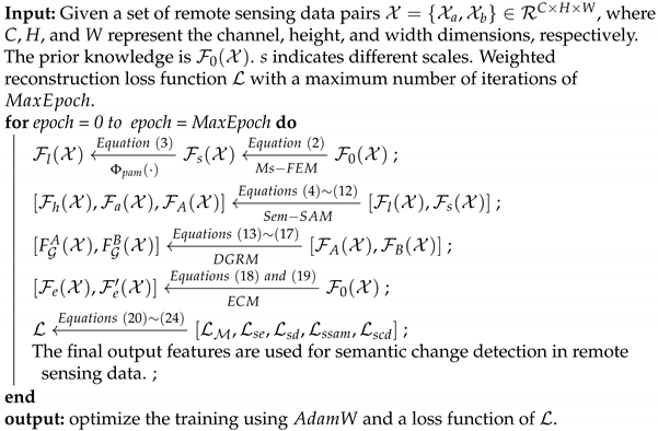
In summary, this weighted loss function can effectively enhance the model’s ability to learn features and simultaneously further ensure semantic consistency in the areas of change in the remote sensing image pairs. The specific operation process is shown in Algorithm 1.

Algorithm 1: The basic operation process of the proposed SDDGRNets.

4. Results

To verify the effectiveness of the proposed SDDGRNets remote sensing data semantic change detection method, we evaluate two datasets: SECOND and HRSCD. In this section, we first introduce the dataset sources, experimental parameters, and evaluation metrics. Then, we provide comprehensive experimental outcomes and an evaluation, and provide example discussions and visualizations.

4.1. Datasets Preparation

SECOND: [11,12] The dataset was collected from multiple platforms and sensors. It contained a total of 4662 pairs of aerial images of $512\times 512$ size, with a resolution ranging from 0.5 m to 3 m, and six semantic land cover categories, including buildings, water bodies, trees, low vegetation, ground, and playgrounds. To guarantee the impartiality of the experiment, these data sets were randomly divided into training, validation, and test at a ratio of 8:1:1.

HIUCD: [13,14] This was mainly used to explore the changes in some parts of Tallinn, the capital of Estonia. It uses ultra-high-resolution images to construct multi-temporal semantic changes to achieve fine semantic change detection. There were 1293 pairs of remote sensing data with a spatial resolution of 0.1m and a size of $1024\times 1024$ for each image, including nine types of target objects, such as water, grassland, woodland, bare land, buildings, greenhouses, roads, bridges, and other. To guarantee the uniformity of the experiment, these data were cropped to $512\times 512$ with a step ratio of 0.1; 80% were used as training samples and 10% as validation samples.

Landsat-SCD: [49] This dataset was derived from Landsat images taken in Tumushuke, Xinjiang, between 1990 and 2020. Tumushuke is located in the “Belt and Road” economic zone, adjacent to the Taklimakan Desert, and has a fragile ecological environment. The dataset comprises numerous complex detection scenes with an unprecedented variety of change types. The study area is adjacent to the desert’s edge, and the buildings within it are small and scattered. The data source consisted of a series of Landsat images with a 30 m resolution. The dataset contained multiple categories, such as ‘farmland’, ‘desert’, ‘buildings’, ‘water body’, etc., and there was also an imbalance problem.

4.2. Parameter Settings

For the remote sensing semantic change detection framework of SDDGRNets, throughout the learning process, the starting learning rate is configured to $0.0001$, the decay rate is configured to $0.00001$, the batch is configured to 32, and the iteration number is configured to 100. AdamW is the optimizer that prevents the architecture from converging to local minima throughout the learning process. Cosine Annealing Warm Restarts is used to adjust the learning rate dynamically.

Furthermore, to guarantee the uniformity and effectiveness of the experiment, all semantic change detection methods were developed on Python 3.8.8 of Ubuntu 20, and trained and tested on an 8-card RTX4090. Additional necessary deep learning frameworks included PyTorch 1.13.0+cu117, Torchvision 0.14.0+cu117, Numpy, and GDAL.

4.3. Metrics

In this study, considering the class imbalance problem, mean intersection over union (mIOU), separable Kappa, and SCD score were used as evaluation indicators. The following Equation (25) shows the specific calculation of mIOU:

$$\left\{\begin{array}{c}mIOU={\displaystyle \frac{1}{\mathcal{M}}}·{\displaystyle \frac{TP}{TP+FP+FN}}\hfill \\ mIO{U}_b=0.5\ast ({\displaystyle \frac{TN}{TN+FP+FN}}+{\displaystyle \frac{TP}{TP+FP+FN}})\hfill \end{array}\right.$$

(25)

where $TP$ denotes a true positive; $FP$ denotes a false positive; $FN$ denotes a false negative; $TN$ denotes a true negative; $\mathcal{M}$ denotes the number of semantic categories; $mIO{U}_b$ indicates the intersection between changed and unchanged. The Equation (26) shows the specific calculation for separable Kappa:

$$\left\{\begin{array}{c}Kappa={\displaystyle \frac{{\mathcal{P}}_0-{\mathcal{P}}_e}{1-{\mathcal{P}}_e}}\hfill \\ SeK=Kappa\times e^{IO{U}_c-1}\hfill \\ {\mathcal{P}}_0={\displaystyle \frac{TP+TN}{TP+TN+FP+FN}}\hfill \\ {\mathcal{P}}_e={\displaystyle \frac{(TP+FP)(TP+FN)+(FP+TN)(FN+TN)}{{(TP+TN+FP+FN)}^2}}\hfill \end{array}\right.$$

(26)

where e represents the exponent; $IO{U}_c$ indicates the intersection-over-union ratio of the changed region. The following Equation (27) shows the specific calculation of $SCDscore$:

$$SCDscore=\beta \times mIO{U}_b+(1-\beta )\times SeK$$

(27)

where $\beta$ indicates the balance parameter $\beta =0.3$.

A comparison with semantic change detection methods is presented in the following section.

4.4. Comparison with Different Methods

To demonstrate the advancement of the proposed SDDGRNets remote sensing image semantic change detection framework, we evaluated all methods on three datasets: SECOND, HIUCD, and Landsat-SCD. The experimental results of various semantic change detection methods are shown in

Table 1. Experimental results of different semantic change detection methods. SDDGRNets is our proposed remote sensing semantic change detection framework. The bold part denotes good performance.

Model-Datasets	SECOND			HIUCD			Landsat-SCD
	mIOU	SeK	SCD-Score	mIOU	SeK	SCD-Score	mIOU	SeK	SCD-Score
HBSCD	72.07	17.63	32.93	75.99	61.32	69.48	73.12	18.19	59.21
SCDNet [10]	72.85	18.42	33.71	90.53	79.88	84.35	75.86	19.36	60.19
LSAFNet [50]	73.65	19.51	34.85	95.90	91.37	93.30	76.42	20.04	61.38
SCanNet	73.05	19.24	34.60	94.24	87.89	90.57	76.87	22.11	61.97
FTA-Net [5]	73.49	19.37	35.04	96.17	92.11	94.55	76.91	22.59	63.31
BiASNet [51]	73.81	19.89	35.29	97.01	92.97	95.36	77.27	24.07	64.19
Amfnet [52]	73.92	20.02	35.43	97.22	83.32	96.08	77.84	24.83	65.72
SDDGRNets	74.32	20.31	35.65	98.99	97.84	98.33	78.92	27.72	67.29

.

From Table 1, the following conclusions can be obtained:

(1) The proposed SDDGRNets remote sensing image semantic change detection framework achieved the best performance in all indicators. On the SECOND datasets, mIOU was improved by 1.27% and 0.67% compared with the SCanNet and LSAFNet methods, respectively. On the HIUCD datasets, the SeK and SCD score were improved by 6.47% and 5.03%, respectively, compared with LSAFANet. On the Landsat-SCD datasets, mIOU is improved by 2.01% and 1.04% compared to FTA-Net and Amfnet, respectively, and SeK is improved by 3.65% and 2.89% compared to BiASNet and Amfnet, respectively. There are two main reasons for this. Firstly, the multi-scale feature extraction module aggregates the basic attribute semantics, such as low-level physical appearance and high-order multi-scale local spatial details. Additionally, the semantic aggregation of the change details of remote sensing data in different phases is carried out, and the representation of significant features is strengthened through the reduction in redundant information transmission. Secondly, the areas of change in the remote sensing data at different phases are encoded separately, strengthening the representation of semantic details in the context of global features. Additionally, the encoded information is decoded layer by layer, and the fusion and propagation capabilities of nodes in the dynamic graph reasoning module are used to further strengthen the interaction between pixels in the neighborhood and establish effective dependencies between channels. In addition, the edge constraint module effectively controls the semantic ambiguity of boundary pixels and the weighted loss function supervises the training of each module separately so that the network can obtain the optimal adjustment function representation and semantic change detection performance.

(2) The HBSCD method achieved the worst detection performance for the SECOND datasets and HIUCD datasets. mIOU was reduced by 0.78% and 14.54%, respectively, compared with the SCDNet method. SeK was reduced by 0.79% and 18.56%, respectively. The SCDNet method uses dual branches to model remote sensing data in different phases. It uses weight-sharing in the encoding stage to better correct deviations in the position information for targets in the same position, thereby achieving a better semantic change detection performance. This shows that weight-sharing in the multi-scale feature extraction stage improves the detection performance of the model. In addition, the evaluation indicators of all methods on the HIUCD dataset differ from those on the SECOND dataset. This may be due to the SECOND dataset’s severe class imbalance and the low spatial resolution of its images. The differences between different categories in the HIUCD dataset are more obvious, which prompts the network to better learn boundary information. This illustrates the importance of edge semantic information for semantic change detection.

(3) Compared with the SCanNet method, the LSAFNet method achieved a good, competitive performance on the SECOND and HIUCD datasets. For example, on the SECOND datasets, SeK and SCD score improved by 0.27% and 0.25%, respectively, compared with the SCanNet method. On the HIUCD datasets, mIOU and SeK improved by 1.66% and 3.48%, respectively, compared with the SCanNet method. The LSAFNet method uses the semantic fusion strategy to filter the initial multi-scale features, diminish the utilization of redundant information, and strengthen the representation of significant features, increasing the model’s performance. Meanwhile, the secondary encoding and decoding method is used to reshape and optimize the detailed information of the ground objects within the region of alteration in the remote sensing data from various temporal sequences, thereby improving the semantic change detection performance. This further shows that semantic screening, secondary encoding, and decoding can enhance the model’s performance.

(4) In the SECOND datasets, the SCD score of the Amfnet method is 0.43% and 0.87% superior to that of the FTA-Net and SCanNet methods, respectively. The Sek of the BiASNet method is 1.47% and 0.52% superior to that of the SCDNet and FTA-Net methods, respectively. On the Landsat-SCD dataset, the mIOU of the FTA-Net method is 0.36% and 0.93% lower than that of the BiASNet and Amfnet methods, respectively. The Sek of Amfnet is 5.61% and 7.68% superior to that of the SCanNet and LSAFNet methods, respectively. This demonstrates that the use of attention mechanisms and multi-scale strategies in the feature extraction phase is advantageous for representing changing targets in the Landsat-SCD dataset. It also further demonstrates that using different branches with weight-sharing to model changing targets in remote sensing data enables the network to perceive subtle changes in an object.

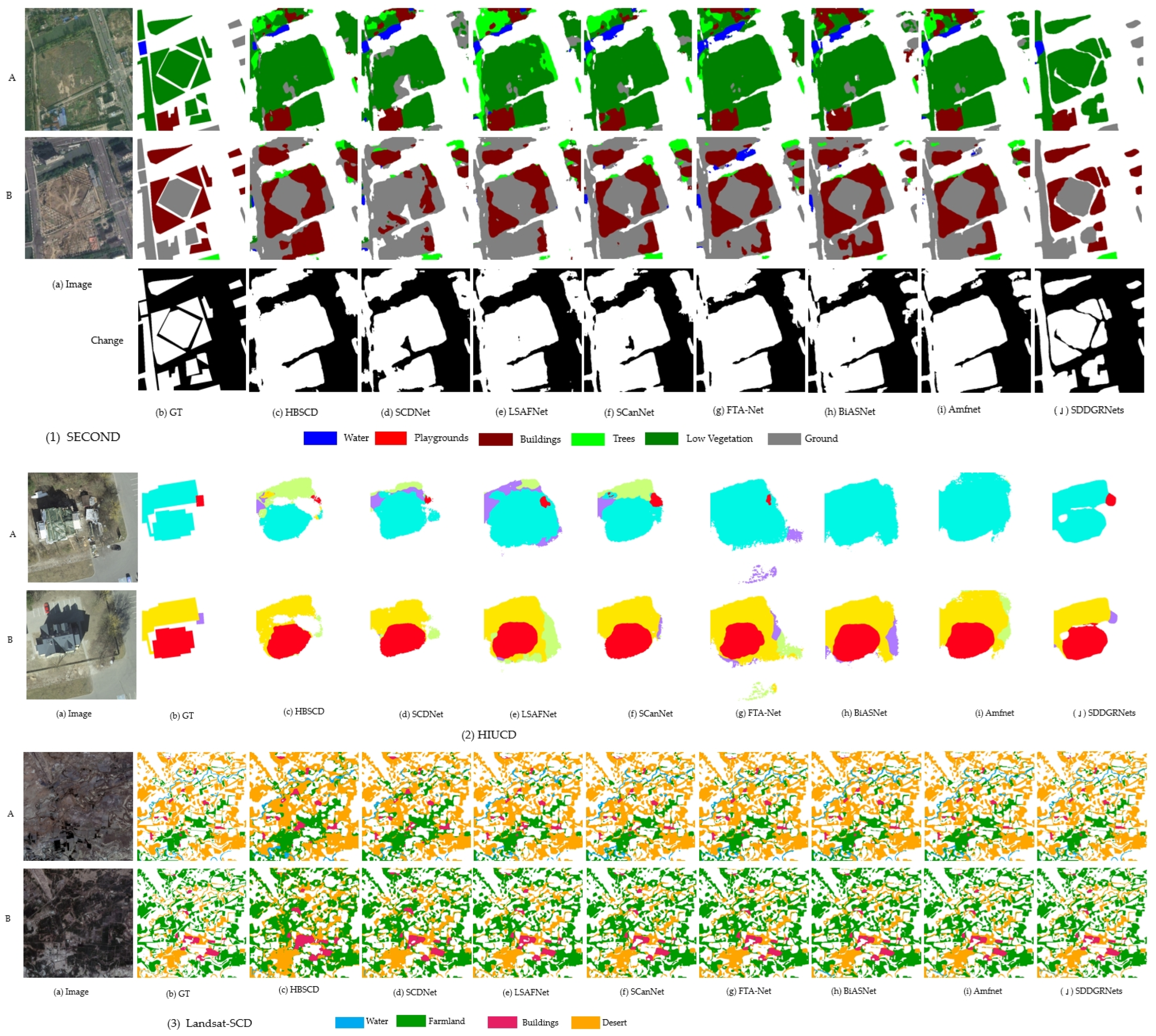
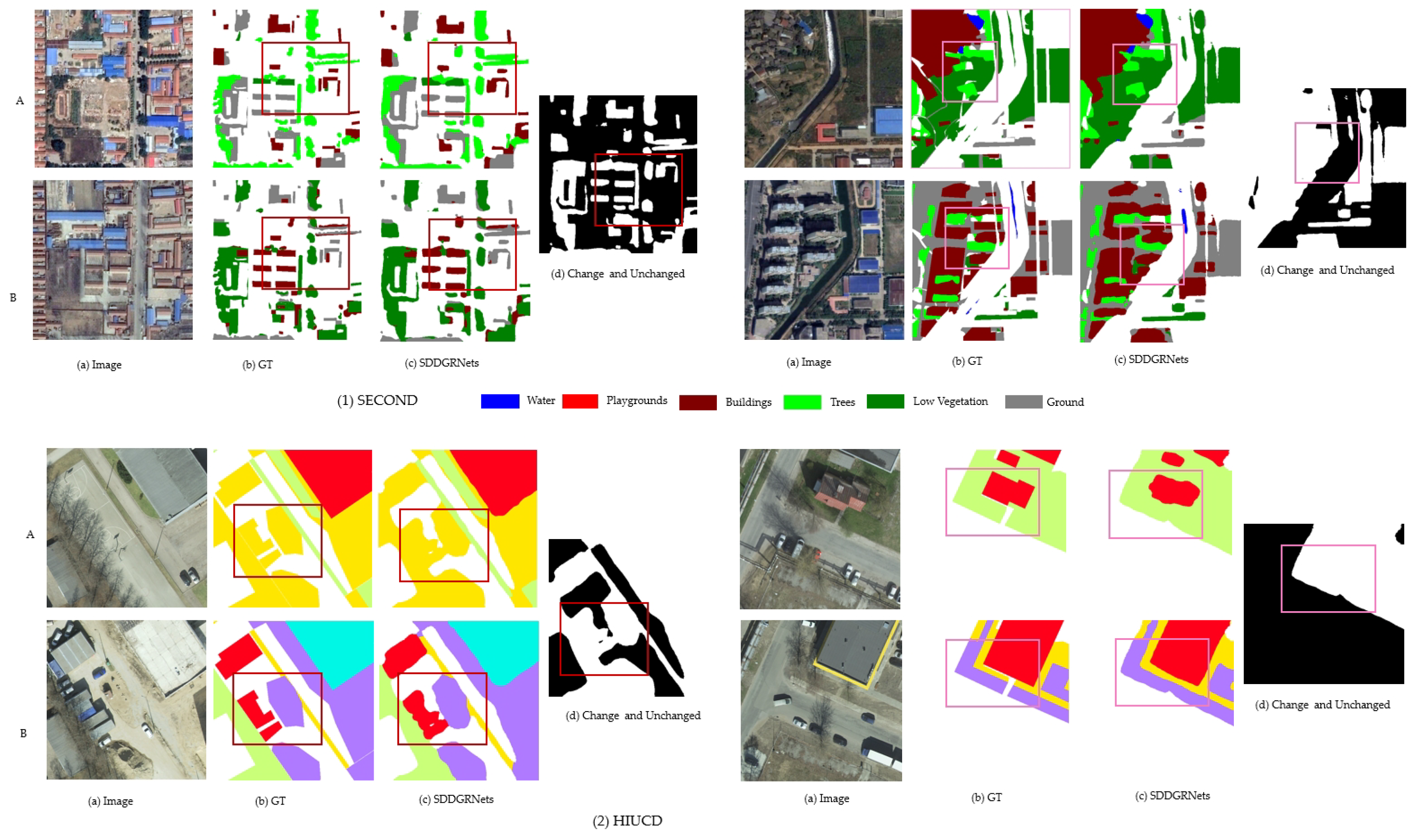
Figure 2 visually demonstrates the different detection methods to demonstrate the effectiveness of the proposed SDDGRNets remote sensing image semantic change detection.

From Figure 2, we can see that the proposed SDDGRNets semantic change detection method achieves the best visualization effect (see Table 1 for specific results). The proposed method not only obtains multi-scale feature details through weight-sharing, but also reduces the differences between features of different scales through the multi-scale aggregation module, thereby improving the representation of features. In addition, the dynamic graph reasoning module and edge constraint module are utilized to more accurately perceive subtle changes in the target within the area of change, thereby improving the semantic representation of the boundary pixels between the alteration region and the adjacent tissue architecture. As shown in Figure 2 (1), in the SECOND dataset, the Low-Vegetation target changes to the Ground target, indicating that the proposed SDDGRNets semantic change detection method exhibits better edge constraint performance.

4.5. Ablation Results

To prove whether the use of multiple modules in the proposed SDDGRNets remote sensing image semantic change detection method plays a positive role in the model’s overall performance, ablation verification was performed on three open-source datasets: SECOND, HIUCD, and Landsat-SCD. The relevant experimental results and an analytical discussion are presented.

Table 2. Experimental results of different modules using the proposed SDDGRNets framework. Ms-FEM stands for multi-scale feature extraction module; Sem-SAM stands for semantic selection aggregation module; DGRM stands for dynamic graph reasoning module; ECM stands for edge constraint module; Ms-FEM+Sem-SAM+DGRM+ECM, Ms-FEM+Sem-SAM+ECM+DGRM, and Ms-FEM+ECM+Sem-SAM+DGRM indicate that the order of the combination of modules is inconsistent. For example, the Ms-FEM+ECM+Sem-SAM+DGRM method entails using Ms-FEM and ECM first, followed by Sem-SAM and DGRM. SDDGRNets is our proposed remote sensing semantic change detection framework; this includes all modules. The bold type indicates the best performance.

Model-Datasets	SECOND			HIUCD			Landsat-SCD
	mIOU	SeK	SCD-Score	mIOU	SeK	SCD-Score	mIOU	SeK	SCD-Score
Ms-FEM	70.80	18.25	33.94	96.54	92.50	94.18	71.32	23.58	62.39
Ms-FEM+Sem-SAM	71.38	18.77	34.38	97.21	94.46	95.70	74.19	25.19	64.82
Ms-FEM+Sem-SAM+ECM	72.11	18.88	34.48	97.81	95.54	96.54	74.88	25.67	65.54
Ms-FEM+Sem-SAM+DGRM	72.43	18.94	34.51	98.05	95.98	96.88	75.39	25.98	65.92
Ms-FEM+Sem-SAM+DGRM+ECM	72.88	19.35	34.92	98.60	97.12	97.77	77.67	26.91	66.83
Ms-FEM+Sem-SAM+ECM+DGRM	72.59	19.11	34.67	98.19	96.83	97.09	76.68	26.29	66.34
Ms-FEM+ECM+Sem-SAM+DGRM	72.68	19.24	34.89	98.33	97.06	97.62	77.49	26.88	66.57
SDDGRNets	74.32	20.31	35.65	98.99	97.84	98.33	78.92	27.72	67.29

shows the semantic change detection performance of different modules.

According to the ablation experiment results in Table 2, the following conclusions can be obtained:

(1) Instead of using a simple module combination or a single module, only when each module cooperates can the network achieve the best semantic change detection performance. For example, in the SECOND dataset, the SeK of the SDDGRNets method with multi-module cooperation is 0.96% and 1.37% superior to that of the Ms-FEM+Sem-SAM+DGRM+ECM and Ms-FEM+Sem-SAM+ECM methods, respectively. In the HIUCD dataset, the SCD score of the SDDGRNets method is 1.45% and 4.15% superior to that of Ms-FEM+Sem-SAM+DGRM and Ms-FEM methods, respectively. In the Landsat-SCD dataset, the mIOU of the SDDGRNets method is 3.53% and 4.73% superior to that of the Ms-FEM+Sem-SAM+DGRM and Ms-FEM+Sem-SAM methods, respectively. Sek is 0.81% and 4.14% superior to that of the Ms-FEM+Sem-SAM+DGRM+ECM and Ms-FEM methods, respectively. A possible reason for this is that employing an individual loss function to supervise the learning of multiple modules enables each module to obtain optimal semantic features, significantly improving the semantic change detection performance of remote sensing data. It also demonstrates that cooperation among various components can allow the network to achieve a superior performance.

(2) Compared with other semantic change detection methods with multi-module combinations, the single-module Ms-FEM achieved the worst detection performance on both the SECOND and HIUCD datasets. For example, the mIOU of the Ms-FEM+Sem-SAM method is 0.58% and 0.67% superior to that of Ms-FEM. This shows that the effectiveness of semantic change detection can be effectively enhanced through semantically screening and re-aggregating the multi-scale local spatial features that are initially obtained. The SeK of the Ms-FEM+Sem-SAM+ECM method is 0.11% and 1.08% superior to that of the Ms-FEM+Sem-SAM method. This demonstrates that using the boundary constraint module can enhance the semantic representation ability of boundary pixels. It can also reduce the semantic ambiguity of boundary pixels, thereby improving the final semantic change detection performance.

(3) In the HIUCD dataset, the SCD score of the Ms-FEM+Sem-SAM+DGRM+ECM method is 0.89% and 1.23% superior to that of the Ms-FEM+Sem-SAM+DGRM and Ms-FEM+Sem-SAM+ECM methods, respectively. In the SECOND datasets, the mIOU and SeK of the Ms-FEM+Sem-SAM+DGRM method are 0.32% and 0.06% superior to those of the Ms-FEM+Sem-SAM+ECM method, respectively. In the Landsat-SCD datasets, the mIOU and Sek of the Ms-FEM+Sem-SAM+DGRM method are improved by 0.51% and 0.31% respectively, compared with the Ms-FEM+Sem-SAM+ECM method. This shows that the dynamic graph reasoning strategy in the semantic re-aggregation stage can effectively enhance the decoding ability of semantic information.

(4) In all semantic change detection datasets, different detection performances were shown when multiple modules were combined in inconsistent orders. In the second dataset, the SCD score of the Ms-FEM+Sem-SAM+ECM+DGRM and Ms-FEM+ECM+Sem-SAM+DGRM methods was 0.03% and 0.25% lower, respectively, than that of Ms-FEM+Sem-SAM+DGRM+ECM. In the Landsat-SCD datasets, the mIOU and Sek of the Ms-FEM+Sem-SAM+DGRM+ECM method were 0.99% and 0.62% higher, respectively, than those of the Ms-FEM+Sem-SAM+ECM+DGRM method. In the HIUCD dataset, the Sek and SCD score of the Ms-FEM+Sem-SAM+DGRM+ECM method are 0.06% and 0.15% superior to those of the Ms-FEM+ECM+Sem-SAM+DGRM method, respectively. The combination of different orders of modules affects the network’s ability to extract detailed features from remote sensing image pairs, resulting in varying detection performance.

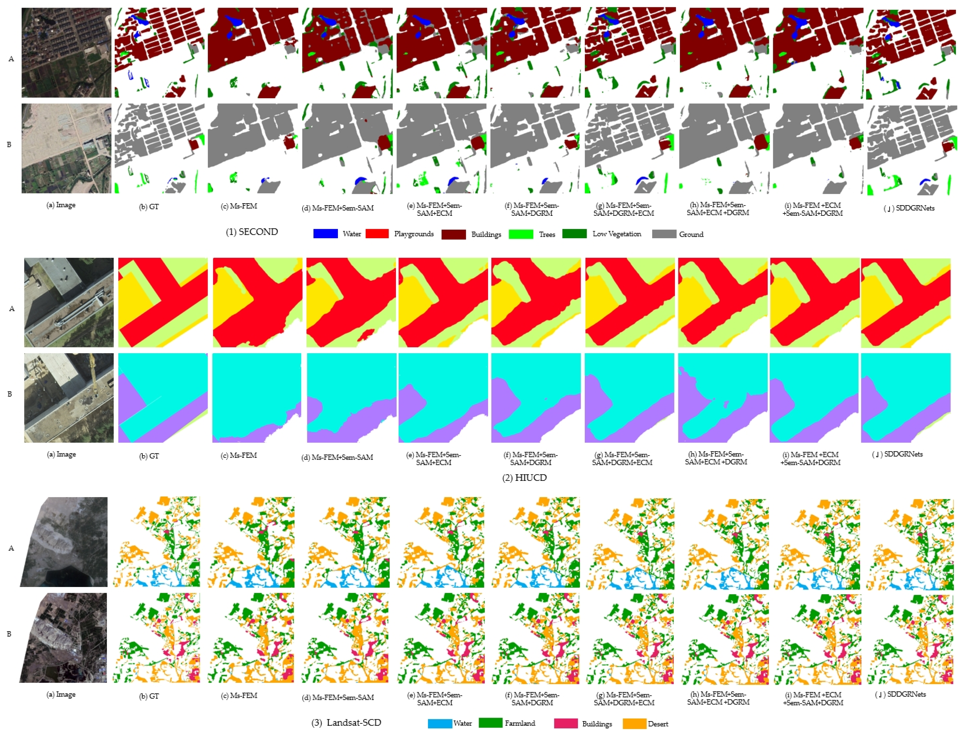
To intuitively demonstrate the effectiveness and detection performance of each module, Figure 3 provides a visual of the different modules.

Figure 3 shows that only when the modules cooperate can a better detection performance be achieved. The Ms-FEM method has the worst visualization effect on the three datasets. This method only extracts the multi-scale features of semantically changing targets. It does not account for differences among the features of various scales throughout the integration phase, resulting in the worst visualization performance.

4.6. Example Discussion

4.6.1. Efficiency Discussion

The effectiveness of semantic change detection methods, including detection results, time efficiency, and model complexity, are critical indicators to consider when determining whether a method is qualified. Therefore, to further demonstrate the practicality and reliability of the proposed SDDGRNets remote sensing image semantic change detection framework, FLOPs and model parameters are used as calculation indicators of time efficiency and model complexity. See Figure 4 for details.

Figure 4 shows that the HBSCD and SCDNet remote sensing image semantic change detection methods have higher reasoning speed and lower model complexity; FLOPs are 12.4 G and 17.3 G, respectively. However, the semantic change detection performance is poor (see Table 1 for results). Although the LSAFNet and SCanNet semantic change detection methods can effectively capture the spatial semantic details of the changed area in the remote sensing image and achieve good detection performance, their time efficiency is poor and difficult to use on a large scale; FLOPs are 35.6 G and 26.8 G, respectively. This study proposes that the SDDGRNets remote sensing image semantic change detection can meet the application requirements well when accuracy is ensured, and the reasoning efficiency and model complexity can also meet the application requirements well, with a FLOPs and Param of 22.3 G and 498 M, respectively. This further proves that the proposed remote sensing image semantic change detection is reliable.

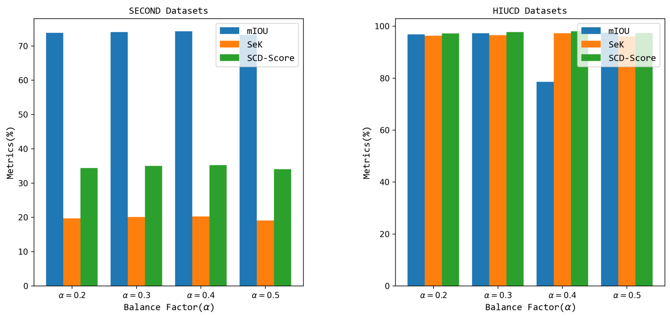
4.6.2. Weight Factor

The effectiveness of the proposed weighted loss function and the impact of the balance factor $\alpha$ in the loss function affect the model’s performance. To verify the rationality and adaptability of the balance factor, the range of the balance factor $\alpha$ was set to $\alpha =\{0.2,0.3,0.4,0.5\}$ for verification. The semantic change detection performance of different balance factors is shown in Figure 5.

Figure 5 shows that with an increase in the weight factor $\alpha$, the performance of the proposed SDDGRNets remote sensing image semantic change detection framework first increases and then decreases. The semantic change detection performance achieves better results when $\alpha =0.4$. For example, in the SECOND dataset, mIOU and Sek are 74.26 and 20.23, respectively, 0.25 and 0.14 superior to when $\alpha =0.3$. In the HIUCD dataset, the SeK and SCD score of $\alpha =0.5$ are 0.45 and 0.63 lower than when $\alpha =0.3$. A possible reason for this is that an excessively high balance factor causes the semantic selection aggregation module to fall into a local optimal state, which struggles to learn the detailed semantic information of the ground objects in the area of change in remote sensing data of different phases. It is worth noting that the balance factor $\alpha$ in this study is $\alpha =0.45$.

4.6.3. Examples of Different Scales

To verification the effectiveness of SDDGRNets framework on objects of varying scales across different datasets, Figure 6 provides a visual representation of the datasets.

In Figure 6, the proposed SDDGRNets semantic change detection framework is shown to better obtain the detailed semantics of large-scale targets, but has weaker modeling capabilities for small-scale targets (see the red box and light red box in Figure 6). A possible reason for this is that the outline of large-scale targets is more precise, and the proposed network enhances the feature representation capability of large-scale targets by transferring shallow features and implementing multi-scale aggregation.

5. Conclusions

In this study, we proposed an SDDGRNets framework for semantic change detection in remote sensing data. This framework uses large kernel dilation decomposition convolution to obtain multi-scale low-level prior knowledge of ground objects in an area of change in remote sensing data. Dividing the subspace better captures the target’s multi-scale local spatial semantic details. Then, a two-branch semantic selection aggregation module is used to screen and re-aggregate the multi-scale spatial local details, strengthen the dependency between different scale features, and allow for weight-sharing between remote sensing data of different phases. A semantically enhanced visual attention module (MSE-VAN) is employed to encode the aggregated multi-scale semantic information, which improves the network’s perception of global features and contextual semantic information and further strengthens the representation of significant semantics. Then, a newly designed dynamic graph reasoning module is employed to decode the encoded features layer by layer, and the dynamic aggregation and transfer capabilities of the graph inference nodes are employed to establish effective interactions between adjacent pixels in the change area, which improves its semantic encoding and decoding capabilities. A newly designed edge constraint module is employed to constrain boundary pixels to enhance the semantic characterization capability of edge pixels and reduce semantic ambiguity. In addition, the loss functions with different weights are employed to supervise each module’s learning separately, effectively reducing the transmission of cumulative errors. Finally, on two sets of open-source semantic change detection datasets, the proposed framework is compared with a variety of popular methods, and it is demonstrated that our proposed method has an excellent detection performance.

Although the proposed semantic change detection achieved a good performance, we still found the following limitations throughout the experimental study: (1) the balance factor in the newly designed reconstruction loss function in the proposed framework is relatively complex, and multiple experimental demonstrations, as well as sufficient experience, are needed to determine the effectiveness of the balance factor; (2) the constraint and penalty capabilities of the boundary pixels between the changed area and the unchanged region are inadequate, and the representation capability of edge features needs to be further improved; (3) the model complexity is relatively high, and it is necessary to reduce the model complexity while maintaining the detection performance. To address these shortcomings, we will redesign a unified and adaptive loss function in the future that can strongly constrain and penalize the boundary pixels of both the changed and unchanged areas while reducing complexity when setting the balance factor. In addition, a simpler and more efficient dynamic graph semantic learning network will be designed to further diminish the computational burden of the model, better meeting the needs of real-world applications.