A Hybrid ANN–GWR Model for High-Accuracy Precipitation Estimation

Abstract

Multi-source fusion techniques have emerged as cutting-edge approaches for spatial precipitation estimation, yet they face persistent accuracy limitations, particularly under extreme conditions. Machine learning offers new opportunities to improve the precision of these estimates. To bridge this gap, we propose a hybrid artificial neural network–geographically weighted regression (ANN–GWR) model that synergizes event recognition and quantitative estimation. The ANN module dynamically identifies precipitation events through nonlinear pattern learning, while the GWR module captures location-specific relationships between multi-source data for calibrated rainfall quantification. Validated against 60-year historical data (1960–2020) from China’s Yongding River Basin, the model demonstrates superior performance through multi-criteria evaluation. Key results reveal the following: (1) the ANN-driven event detection achieves 10% higher accuracy than GWR, with a 15% enhancement for heavy precipitation events (>50 mm/day) during summer monsoons; (2) the integrated framework improves overall fusion accuracy by more than 10% compared to conventional GWR. This study advances precipitation estimation by introducing an artificial neural network into the event recognition period.

1. Introduction

Precipitation, a critical component of the global hydrological cycle, fundamentally influences climate change, hydrological forecasting, and socio-economic systems through its connections to water resources management and agricultural productivity. The growing demand for high-resolution, long-term precipitation data has intensified scrutiny of current estimation methods, particularly their performance under extreme meteorological conditions where accuracy limitations persist [1,2].

The evolution of spatial precipitation estimation has progressed through three paradigms [3]. The first-generation-stage approaches relied on spatial interpolation techniques (e.g., Kriging, IDW) to extrapolate point-based gauge measurements [4]. While computationally simple, these methods exhibit strong dependence on gauge network density and struggle to capture orographic effects on complex terrains [5]. The second generation leveraged satellite remote sensing (TRMM, GPM) and atmospheric reanalysis to achieve continuous spatiotemporal coverage [6,7,8]. Despite advancements in global monitoring, these datasets face persistent challenges: GPM, while outperforming TRMM in heavy rainfall detection, still underestimates extreme events by 20–40% in mountainous regions [9,10,11]. This accuracy degradation stems from inherent limitations in retrieval algorithms and sensor sensitivity to cloud microphysics.

Emerging as the third paradigm, multi-source data fusion integrates ground observations, satellite retrievals, and atmospheric modeling to reconcile scale mismatches and reduce systematic biases [12,13,14,15,16,17]. Among fusion techniques, geographically weighted regression (GWR) has gained prominence for its ability to model spatial non-stationarity by establishing location-specific regression relationships [18]. However, our analysis reveals two critical limitations in current GWR implementations: (1) inadequate handling of precipitation event detection thresholds, leading to false alarms (FAR >35% in summer monsoon periods); (2) linear regression assumptions that fail to capture nonlinear interactions between topographic variables and precipitation intensity. These shortcomings persist despite improved data availability, suggesting structural constraints in traditional fusion frameworks.

Recent breakthroughs in machine learning present transformative opportunities [19,20,21]. Artificial neural networks (ANNs) have demonstrated superior performance in precipitation classification through hierarchical feature extraction from heterogeneous inputs [22,23]. Unlike conventional threshold-based methods, ANN architectures can learn complex decision boundaries between rain/no-rain states while incorporating ancillary variables (elevation, potential evapotranspiration) as nonlinear predictors [24,25]. Nevertheless, standalone machine learning models often lack explicit mechanisms to address spatial heterogeneity—a strength inherent to GWR. This complementarity motivates our hybrid approach: integrating ANN-based event detection with GWR-driven quantitative estimation to synergize their respective advantages.

This study makes two key contributions: (1) it proposes a hybrid ANN–GWR model that decouples precipitation event detection (ANN) from intensity estimation (GWR), addressing the problem of combining ANN for precipitation event detection with traditional GWR for quantitative estimation; (2) it provides systematic validation across precipitation intensity regimes, demonstrating 15% accuracy gains for heavy rainfall (>50 mm/day) through comprehensive error decomposition (hit bias, HB; missed precipitation, MP; false precipitation, FP).

2. Methodology

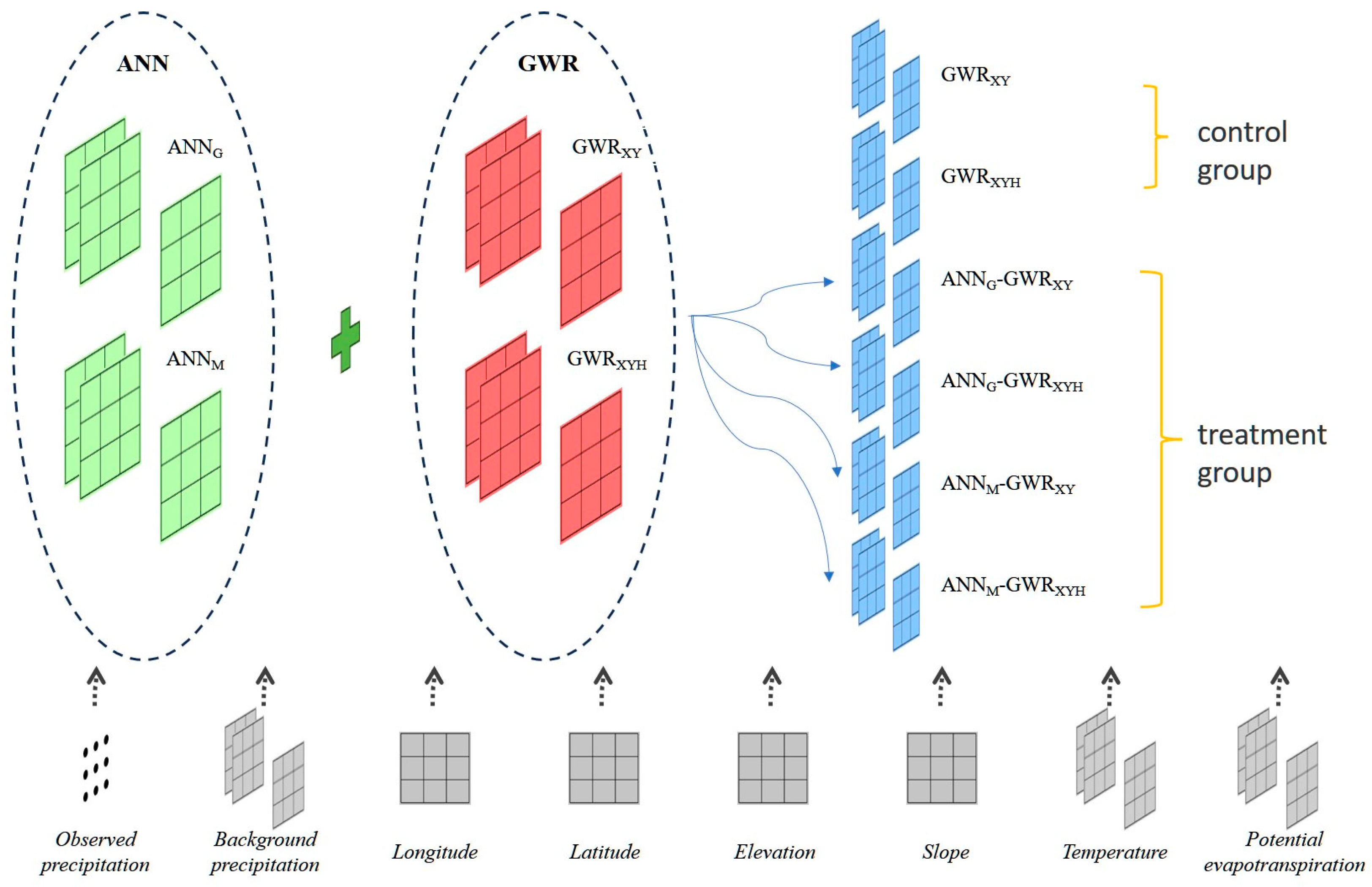
2.1. Integrated ANN–GWR Framwork

The proposed ANN–GWR model operates through three stages (Figure 1): (1) precipitation event detection via ANN, (2) quantitative precipitation estimation using GWR, and (3) error correction through spatial masking and interpolation.

Stage 1: ANN-driven precipitation detection: The identification of rain versus no-rain states is based on an ANN model, which extracts hidden relationships between precipitation states and various factors. This model constructs a probability field for precipitation classification, ultimately generating a grid-based rain/no-rain decision field.

To enhance the accuracy of the ANN model, six input variables are incorporated: geographic information (latitude, longitude), elevation, slope, temperature, and potential evapotranspiration. Additionally, to assess whether the background field precipitation influences the model’s accuracy, background field precipitation is introduced as a seventh input variable.

• Experiment 1: In this setup, the six input variables include geographic information (latitude, longitude), elevation, slope, temperature, and potential evapotranspiration (referred to as ANN_G);
• Experiment 2: This setup incorporates all seven input variables: geographic information (latitude, longitude), elevation, slope, temperature, potential evapotranspiration, and background field precipitation (referred to as ANN_M).

The artificial neural network (ANN) is a type of machine learning method capable of addressing complex regression and classification tasks [26,27]. ANN is structurally divided into three layers: the input layer, the hidden layer, and the output layer. The input layer consists of seven input features, the hidden layer contains 12 nodes, and the output layer includes one output parameter. The ANN’s hyperparameters include the learning rate (0.001), the number of iterations (400), the Dropout rate (0.5), and so on. The core component of an artificial neural network is the artificial neuron. A standard neural network is composed of many “neurons”. The information transmission process of a neuron can be described as follows:

Weight matrix:

$$z^{\left(j\right)}={\theta }^{(j-1)}{a}^{(j-1)}$$

(1)

Activation vector:

$$a^{\left(j\right)}= g(z^{(j-1)})$$

(2)

Activation function:

$$Softmax(Z_j)={\displaystyle \frac{e^{Z_j}}{{\displaystyle {\sum }_{k=1}^K{e}^{Z_k}}}}$$

(3)

Loss function:

$$L\mathrm{oss}=-{\displaystyle \sum _{i=1}^n{y}_i\log ({\widehat{y}}_i)}$$

(4)

Stage 2: GWR-based precipitation quantification: A fusion model is constructed based on the GWR (geographically weighted regression) model to integrate ground-observed precipitation data with the ERA5-land reanalysis dataset. This model provides an initial estimate of precipitation levels for each grid cell. The primary inputs for the GWR model include geographic information (latitude, longitude), background precipitation fields, and ground-observed precipitation. Depending on whether elevation data are included as an input variable, the model is divided into two schemes: GWR_XY and GWR_XYH.

The concept of geographically weighted regression (GWR) was formally introduced by Professor A. Stewart Fotheringham from the University of St Andrews in 1996 [28]. GWR is a spatial statistical method that reveals spatial non-stationarity in geographic phenomena. It generates a local regression model at each location within the study area, allowing for the explanation of local spatial relationships and spatial heterogeneity. For spatially distributed dependent variables like precipitation, mineral concentration, or population density y, suppose there are n observation points and p covariates in the study area. The GWR equation is expressed as follows:

$$y_i={\beta }_0(u_i,v_i)+{\displaystyle \sum _{k=1}^p{\beta }_k(u_i,v_i)}{x}_{ik}+{\epsilon }_i i=1,2,\dots ,n$$

(5)

where $(u_i,v_i)$ represents the coordinates of the ith observation point; ${\beta }_k(u_i,v_i)$ is the kth regression parameter at the ith observation point, which is a function of spatial location; and ${\epsilon }_i$ is the residual error, assuming ${\epsilon }_i~N(0,{\sigma }^2)$ and $Cov({\epsilon }_i,{\epsilon }_j)=0(i\ne j)$. $x_{ik}$ denotes the kth covariate at the ith observation point.

According to the spatial autocorrelation in geography, the regression parameters at adjacent locations are more similar. Based on the spatial positions of each element in the study area, calculate the attenuation function, which is a continuous function. This function can transfer the weights of nearby samples to the unknown point, construct a local weighted regression model at each unknown point based on the known samples, and thereby determine the regression parameters at the unknown point. After substituting the spatial positions of each element into the function, the weight values of the elements can be obtained. This weight value can be brought into the regression equation to calculate the value at the unknown point. According to the least squares method, the derivation formula of the weight value is as follows:

$${\widehat{\mathit{\beta }}}_i(u_i,v_i)={({\mathit{X}}^{\mathit{T}}\mathit{W}(u_i,v_i)\mathit{X})}^{-1}{\mathit{X}}^{\mathit{T}}\mathit{W}(u_i,v_i)y$$

(6)

$$\mathit{W}(u_i,v_i)=diag(w_1(u_i,v_i),w_2(u_i,v_i),\dots ,w_n(u_i,v_i))$$

(7)

where $\stackrel{\wedge }{\mathit{\beta }}$ represents the regression coefficients calculated from known points; X represents the explanatory or independent variables; y represents the dependent variable at the known points, which is used to compute the regression coefficients for unknown points; and W(u_i,v_i) is the spatial weight matrix derived from a decay function.

The spatial weight matrix is given by the following:

$$w_{ij}=\varphi (d_{ij}^2/\sigma {b_S}^2)$$

(8)

where $d_{ij}$ is the distance between the neighboring point j and the center point i; $\varphi$ is the standard normal probability density function; $\sigma$ is the standard deviation of the distances between the neighboring points and the center point i; and b is the spatial bandwidth.

The optimal bandwidth is calculated using the following:

$$CVRSS(b)={\displaystyle \frac{1}{n}}{\displaystyle \sum _{i=1}^n{(y_i-{\widehat{y}}_{\ne i}(b_S))}^2}$$

(9)

where ${\widehat{y}}_{\ne i}(b)$ is the estimated value of the dependent variable at point i based on the regression parameters estimated after excluding point i.

Stage 3: error correction protocol: To correct missed precipitation (MP) and false precipitation (FP) in the grid, the precipitation status grid from Stage 1 is multiplied by the multi-source precipitation fusion results from Stage 2. This multiplication helps refining the precipitation data by aligning the detected rainfall events with the actual precipitation quantities.

It is important to note that the combination of the ANN model and the GWR model can lead to four possible scenarios when they are multiplied together, with 1 representing precipitation and 0 representing no precipitation in the scenarios below:

• Scenario 1: P_ANN = 0 and P_GWR = 1
• Scenario 2: P_ANN = 0 and P_GWR = 0
• Scenario 3: P_ANN = 1 and P_GWR = 1
• Scenario 4: P_ANN = 1 and P_GWR = 0

In the first two scenarios, the results are consistent and correct. The third scenario is also accurate as both models agree on the presence of precipitation. However, the fourth scenario presents a challenge: although the ANN model detects precipitation, the GWR model does not, thus failing to provide precipitation data. To address this, a correction is needed. Specifically, in cases where P_ANN = 1 and P_GWR = 0, the inverse distance weighting (IDW) interpolation method is used to estimate the missing precipitation values by referencing the eight nearest grid cells with detected precipitation.

The detailed scheme of the ANN–GWR multi-source precipitation fusion model is illustrated in Figure 1. The original precipitation data used in the fusion process include ground-based observations and background precipitation fields, typically derived from satellite retrievals and reanalysis datasets. The GWR_XY and GWR_XYH models serve as control groups, and the fusion scheme is divided into four variants based on whether background precipitation data were included in the precipitation classification and whether elevation data were incorporated in the fusion process: ANN_G-GWR_XY, ANN_G-GWR_XYH, ANN_M-GWR_XY, and ANN_M-GWR_XYH.

To evaluate the accuracy of the ANN–GWR model, cross-validation was employed [29]. Suppose there are n ground-based rainfall stations within the study area. Each time, n−1 stations are used as known points (training samples), while the remaining station serves as the validation point (validation sample). This process is repeated for all n stations, and the fusion results from all these calculations are aggregated into a validation set. Finally, the performance of the model is evaluated by comparing the validation set to the actual precipitation data recorded at the stations.

2.2. Validation and Error Decomposition

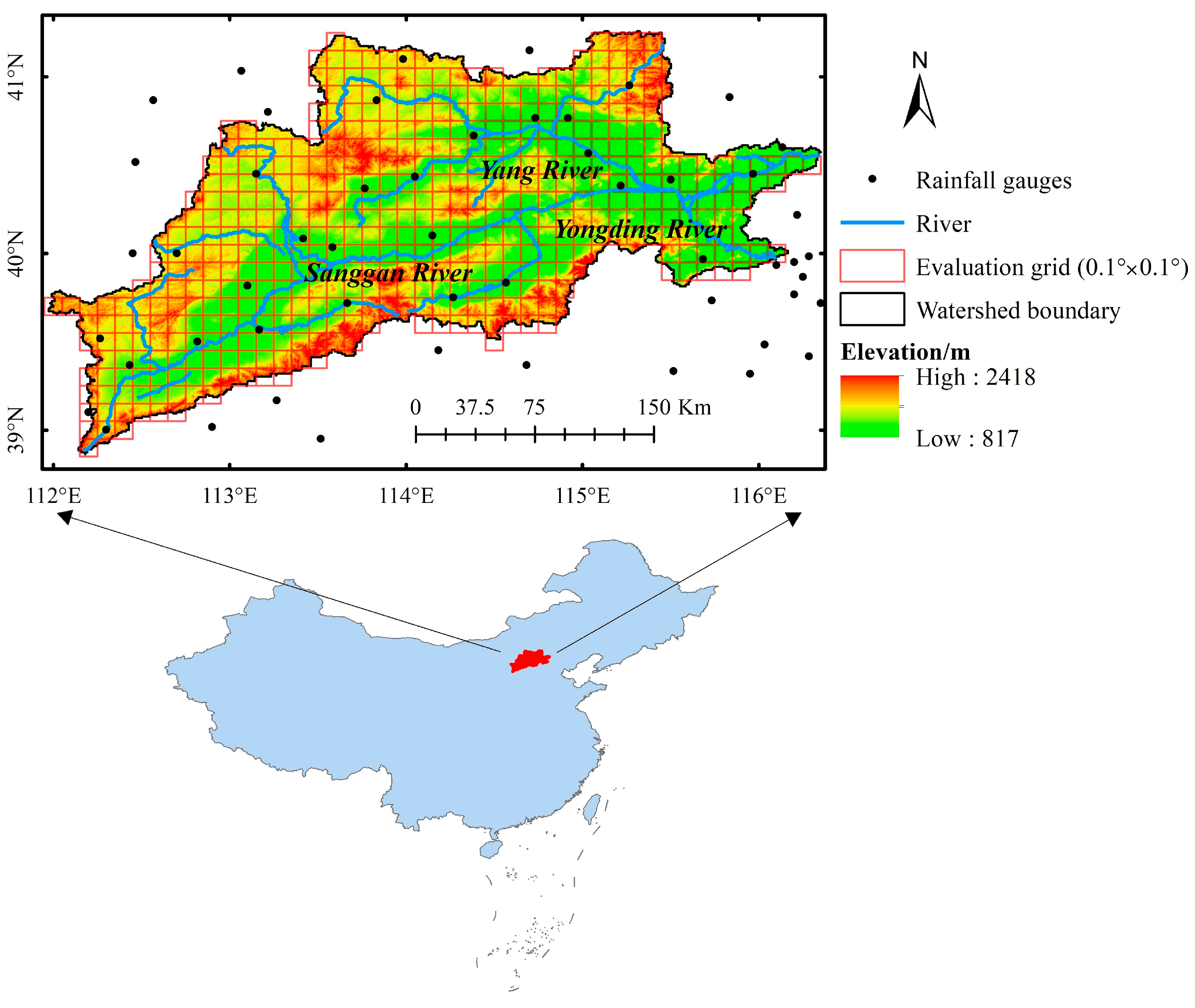
The accuracy evaluation is primarily divided into classification metrics and quantitative metrics [30,31]. For classification metrics, we use the probability of detection (POD), false alarm ratio (FAR), and critical success index (CSI). The quantitative metrics include mean absolute error (MAE), correlation coefficient (CC), and Kling–Gupta efficiency (KGE).

$$KEG=1-\sqrt{{(1-CC)}^2+{(1-\alpha )}^2+{(1-\beta )}^2}$$

(10)

$$a={\mu }_R/{\mu }_{\mathrm{G}}$$

(11)

$$\beta =({\sigma }_R/{\mu }_R)/({\sigma }_G/{\mu }_G)$$

(12)

where μ_R indicates the mean of the fused precipitation, and μ_G represents the mean of the observed precipitation at the stations; σ_R and σ_G represent the standard deviations of the fused precipitation and observed precipitation, respectively.

Total precipitation error reflects the overall overestimation or underestimation of ground precipitation in the estimation results. However, since this metric is the result of balancing a large number of positive and negative errors, it obscures detailed information, particularly the quantitative errors under different classification conditions. The method for decomposing error based on rain/no-rain states was first proposed by Tian et al. [32] and later developed by Yong et al. [33]. This method has been proven effective for tracing the sources of error in satellite-based precipitation estimates. It decomposes the total bias (TB) into three independent components: hit bias (HB), missed precipitation (MP), and false precipitation (FP). Analyzing the structure of the total error and the spatial-temporal characteristics of each error component provides significant insights for improving the accuracy of precipitation estimates and selecting appropriate datasets. This means that the total precipitation bias can be broken down into three independent components, where the absolute values of these components may exceed the total precipitation bias, especially MP and FP, which can offset each other due to their opposite signs.

$$TB=HB+MP+FP$$

(13)

$$P(\overrightarrow{x},t)=\left\{\begin{array}{l}1 \mathrm{if} C(\overrightarrow{x},t) > \mathrm{T}\hfill \\ 0 \mathrm{if} C(\overrightarrow{x},t)=\mathrm{T} \mathrm{or} \mathrm{missing}\hfill \end{array}\right.$$

(14)

$$HB={\displaystyle \sum _{t=1}(R_t-G_t)\cdot P(R_t\ge T)\cdot P(G_t\ge T)}$$

(15)

$$MP={\displaystyle \sum _{t=1}(R_t-G_t)\cdot P(R_t<T)\cdot P(G_t\ge T)}$$

(16)

$$FP={\displaystyle \sum _{t=1}(R_t-G_t)\cdot P(R_t\ge T)\cdot P(G_t<T)}$$

(17)

In the formulas, $P(\overrightarrow{x},t)$ represents the binary precipitation event mask, $C (\overrightarrow{x}, t)$ indicates the precipitation field, and T represents the rain/no-rain threshold. For mathematical derivation, T = 0 is used as the threshold to determine the mask for rain/no-rain events. However, in practical applications, a slightly higher threshold (such as 0.1 mm/day) is often used instead of 0 to determine the mask. R denotes the precipitation amount from the fusion scheme, and G represents the ground-observed precipitation.

The accuracy gain of fused precipitation is a crucial metric for evaluating the effectiveness of precipitation fusion. Based on the characteristics of the indicators, accuracy gain can be categorized into three types: positive-oriented, negative-oriented, and intermediate-optimal. For positive-oriented indicators, higher values are better, with the correlation coefficient (CC) being a representative metric. For negative-oriented indicators, lower values are preferable, with the mean absolute error (MAE) being a representative metric. Intermediate-optimal indicators have a specific optimal value; for example, the optimal values for hit bias (HB) and total bias (TB) are 0, while the optimal values for the mean ratio (α) and coefficient of variation ratio (β) are 1. The classification of each indicator is summarized in

Table 1. General formulas for evaluating the gain in multi-source precipitation fusion.

Type	Gain Calculation Formula	Applicable Indicators
Positive-oriented	$\mathsf{\Delta }Z={\displaystyle \frac{Z\left(P_R\right)-Z\left(P_G\right)}{Z\left(P_G\right)}}\times 100\%$	POD,CSI,MP,CC,KGE
Negative-oriented	$\mathsf{\Delta }Z={\displaystyle \frac{Z\left(P_G\right)-Z\left(P_R\right)}{Z\left(P_G\right)}}\times 100\%$	FAR,FP,MAE
Intermediate-optimal	$\mathsf{\Delta }Z={\displaystyle \frac{\left|Z(P_G)-Z_{BEST}\right|-\left|Z(P_R)-Z_{BEST}\right|}{\left|Z(P_G)-Z_{BEST}\right|}}\times 100\%$	HB,TB,α,β

.

In the formulas: P_R represents the fused precipitation, P_G indicates the reference precipitation, Z represents the evaluation indicator, and Z_BEST represents the optimal value of the indicator.

3. Study Area

3.1. Geographical Setting

The Yongding River Basin (38.90–41.16°N, 111.95–116.22°E), a critical sub-basin of the Haihe River system in northern China, spans five provinces and municipalities, including Beijing and Tianjin. Covering an area of approximately 47,000 km², it contributes 14.7% of the total area of the Haihe River Basin. Its primary upstream tributaries, the Sanggan River and the Yang River, converge to form the Yongding River.

3.2. Climatic Characteristics

The Yongding River Basin exhibits a temperate continental monsoon climate characterized by pronounced seasonal variability. The following is based on 60-year observational records (1960–2019):

• Annual precipitation: 360–650 mm (mean: 486 mm), with 80% concentrated in summer months (June to August);
• Extreme rainfall events: Heavy precipitation (>50 mm/day) occurs 3–5 times annually, primarily during July–August;

Temperature range: −20 °C (winter) to 38 °C (summer), facilitating diverse precipitation phases (snowfall vs. convective storms).

3.3. Data Source and Processing

(1) Meteorological observation data from multiple gauges within the Yongding River Basin and its surrounding areas, each with long-term observation records, were selected as the sources of gauge-based precipitation data (source: https://data.cma.cn/ (accessed on 22 July 2025)). The spatial distribution of these gauges is illustrated in Figure 2. Daily precipitation data from these gauges were collected for the period from 1960 to 2019, spanning 60 years.

(2) Elevation data were sourced from 90 m DEM (source: https://www.resdc.cn/ (accessed on 22 July 2025)), which were resampled and processed into 0.1° × 0.1° grid cells. Slope information was generated from the processed DEM.

(3) Temperature, potential evapotranspiration, and background precipitation data were acquired from the ERA5-land dataset (source: https://cds.climate.copernicus.eu (accessed on 22 July 2025)), which features a temporal resolution of 1 h and a spatial resolution of 0.1° × 0.1°. These data were subsequently aggregated to a daily temporal resolution.

The ANN–GWR precipitation fusion model was applied to perform a fusion experiment on the daily precipitation data for the Yongding River Basin from 1960 to 2019. The resulting data have a temporal resolution of 1 day and a spatial resolution of 0.1° × 0.1°.

4. Results

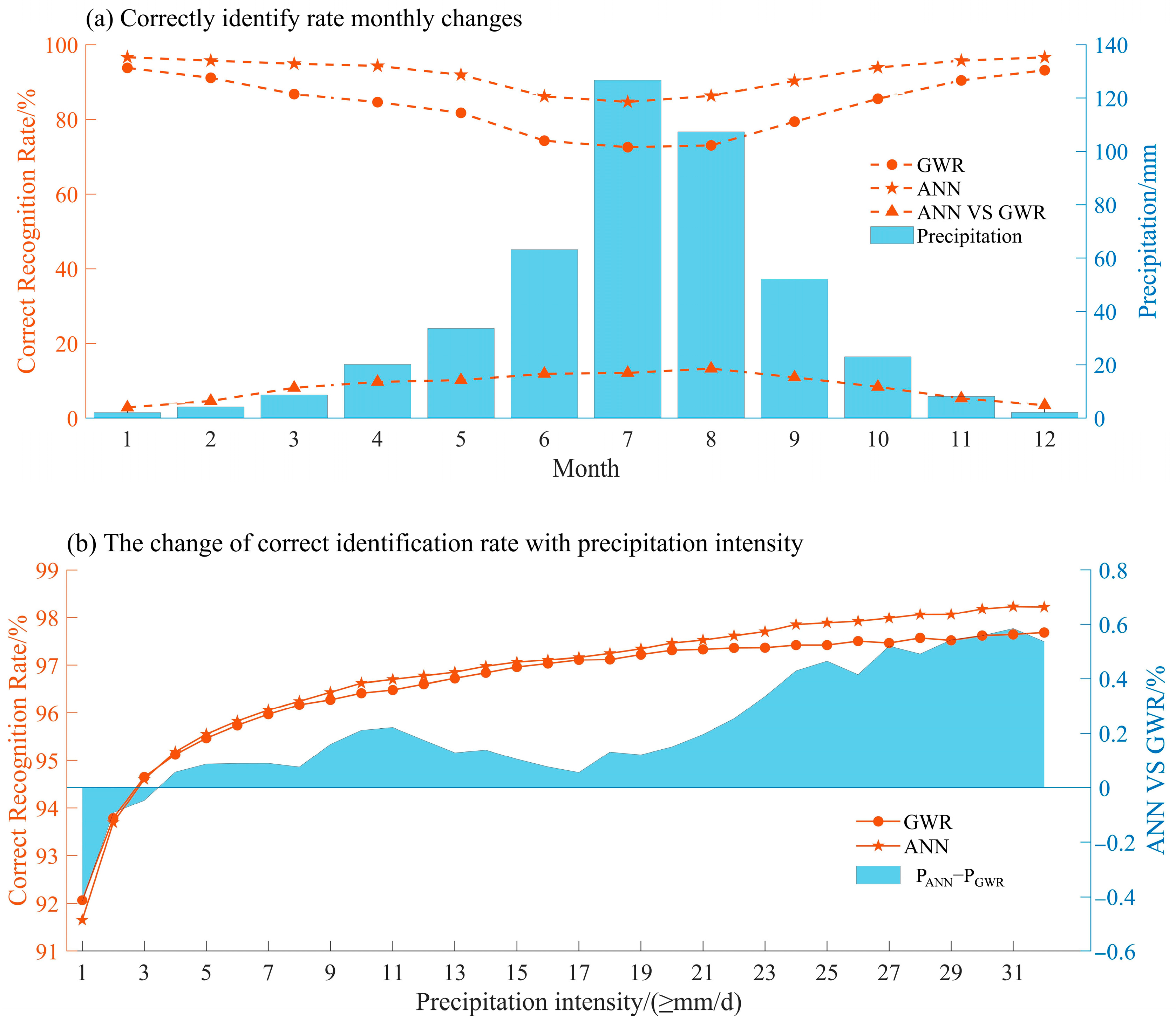
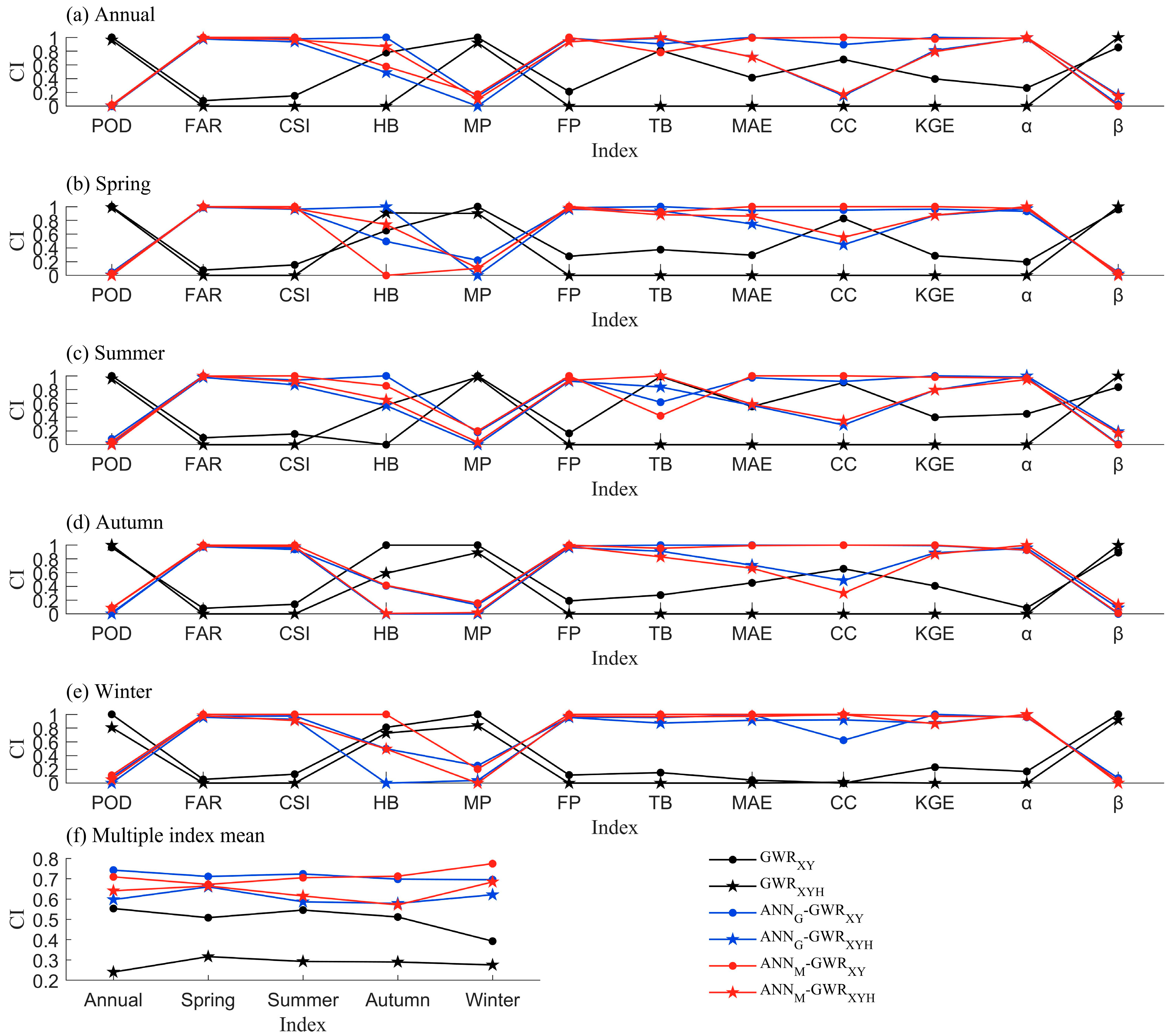
4.1. Accuracy of Precipitation Classification by the ANN Module

Figure 3 shows the spatial distribution of the long-term overall detection rates (the proportion of correctlys identified cases) for each gauge under different models. It reveals that under the ANN model, the average detection rate for both schemes over the 60-year period is consistently above 90%. In contrast, the detection rates for the GWR model range between 80% and 90%, with a significantly lower average over the 60 years compared to the ANN model. This trend indicates that detection rates for both models are closely related to the terrain, with this pattern being particularly evident in the GWR_XY and GWR_XYH schemes. Despite introducing elevation as an additional factor in the GWR_XYH scheme, there was no significant improvement in detection rates compared to the GWR_XY scheme. The reasons for this will be quantitatively analyzed later.

The analysis of average long-term detection rates across gauges shows that the ANN model consistently achieves detection rates above 90%, while the GWR model’s rates are generally below 85%. Both models exhibit a slight upward trend in detection rates over time, which may be related to improvements in observational equipment capturing more detailed information.

Current analysis clearly demonstrates that the ANN module enhances precipitation classification accuracy. However, the impact on the accuracy of precipitation fusion results remains unclear and will be addressed in subsequent sections.

Although the ANN model demonstrates a distinct advantage over the GWR model in precipitation classification, the final ANN–GWR model’s probability of detection (POD) is lower. The analysis of the characteristics of precipitation classification is warranted.

Figure 4a presents the monthly variation in detection rates for the GWR and ANN models. Both models show seasonal variations, with the lowest detection rates in July and the highest in December. The ANN model consistently outperforms the GWR model. The difference between the models, P_ANN–P_GWR (where P represents the correct detection rate), also exhibits a seasonal pattern, peaking in July with a 15% difference. After calculating the monthly and multi-year average precipitation, it is found that the statistical results and the detection rates of the model align with the cyclical variation of PANN–PGWR. June, July, and August, which are summer months in the study area, have the lowest detection rates for both models and the highest P_ANN–P_GWR values. This suggests that precipitation intensity may contribute to these observations.

Figure 4b illustrates the relationship between detection rates and precipitation intensity for both GWR and ANN models. Detection rates increase with precipitation intensity for both models, but there is a notable crossover point (P = 3.8 mm/d). Before this point, the GWR model performs better, while after this point, the ANN model’s performance surpasses that of the GWR model. The variation in P_ANN–P_GWR with precipitation intensity indicates that the ANN model performs better for moderate to high precipitation levels. Statistical data on rainy events show that events with 0.1 mm < P ≤ 3.8 mm account for 63.8% of events with P > 0.1 mm, and their proportion decreases rapidly with increasing precipitation intensity. Thus, it can be concluded that the distribution of detection rates for GWR and ANN models with precipitation intensity contributes to the lower POD of the ANN model.

However, POD alone cannot fully assess the model’s effectiveness. According to the calculation formula, POD = P(G > 0.1 mm and S > 0.1 mm)/P(G > 0.1 mm) (where G and S represent reference and computed precipitation, respectively), the higher POD for the GWR model is due to its better detection rate for events with 0.1 mm < P ≤ 3.8 mm, which constitute 63.8% of rainy events. The volume percentage of these events is only 12.7%, which explains why other metrics perform better in the ANN–GWR model. Figure 4a also shows that the ANN–GWR model has a higher overall detection rate.

The nonlinear ANN model can express the complex interaction that the GWR model has difficulty to capturing, so it can improve the identification rate of precipitation. Although the overall POD is reduced, the POD of heavy precipitation (P > 3.8 mm) is enhanced and the FAR is significantly reduced.

To address these issues, one potential approach is to replace the single ANN and GWR models with multiple models and then integrate them using Bayesian model averaging (BMA). This approach helps mitigate the limitations of individual models and explicitly accounts for the uncertainty in each model’s predictions, constructing a predictive distribution rather than relying solely on deterministic weighted averages [34].

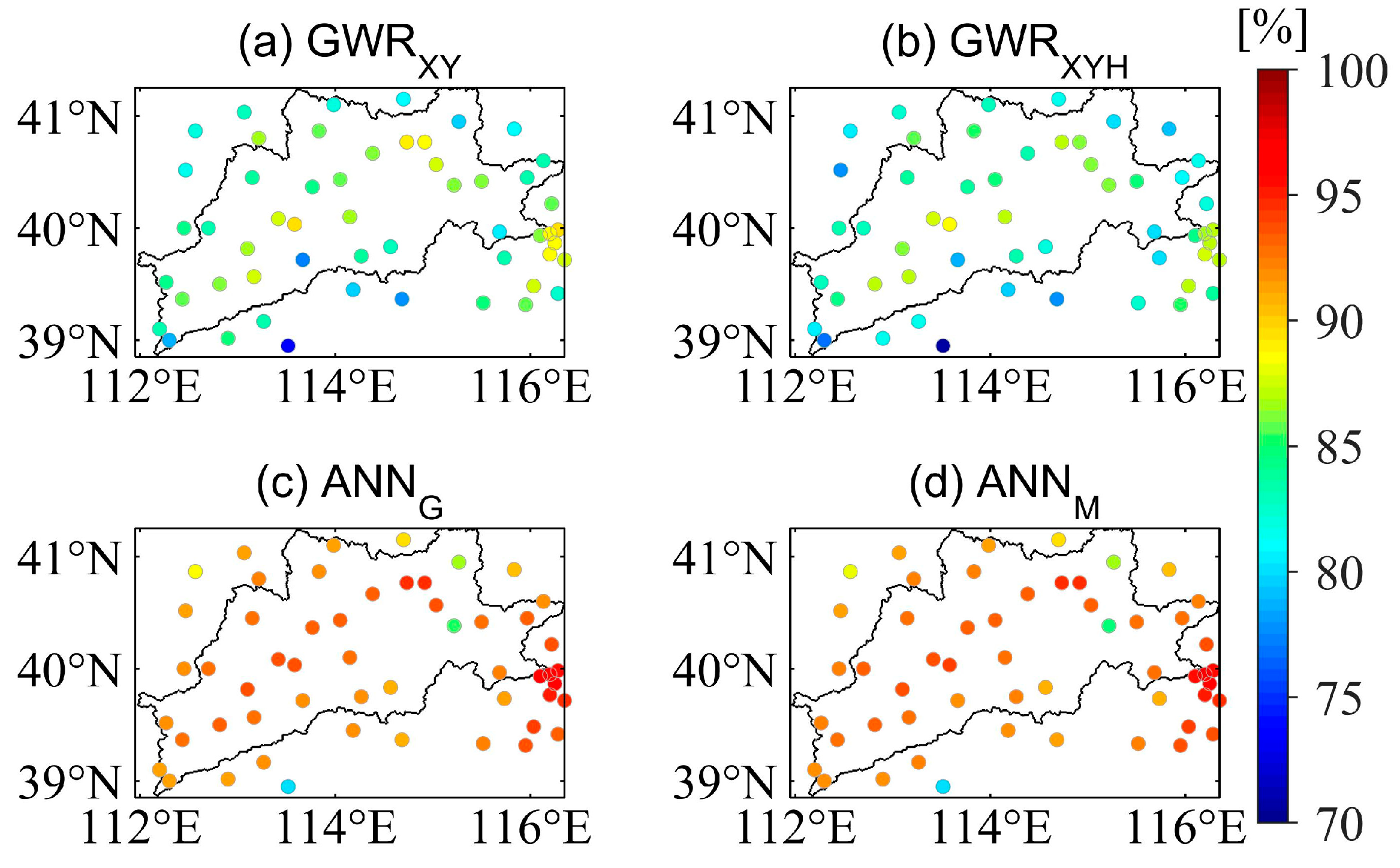
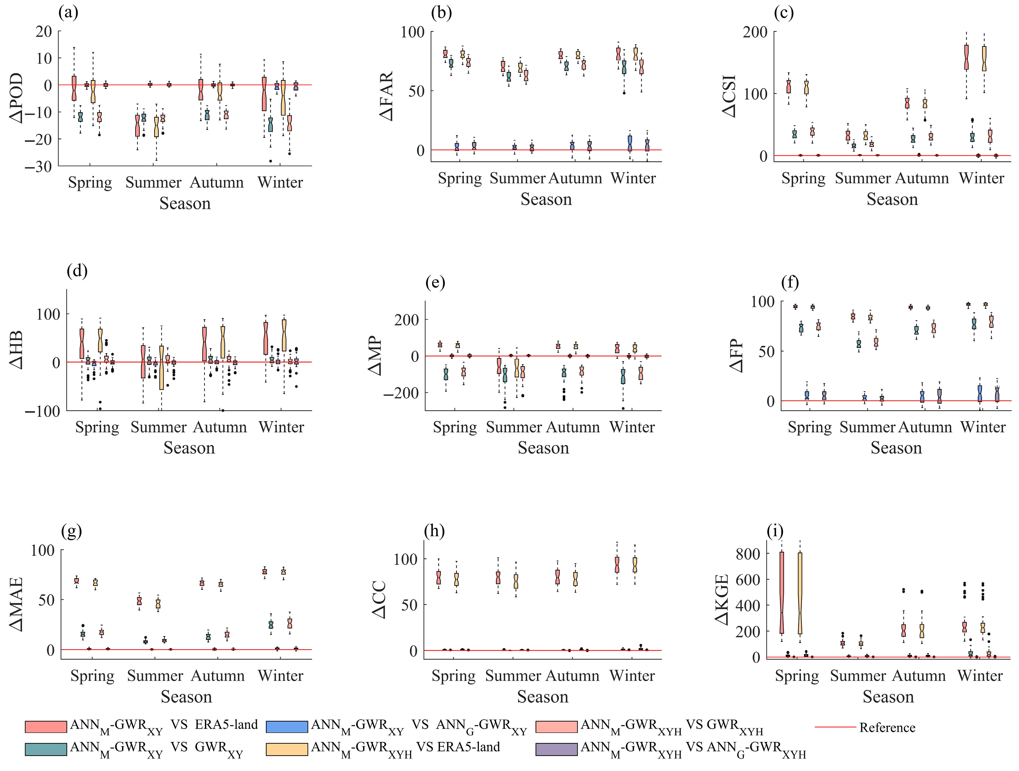
4.2. Gain of ANN–GWR Model Compared to GWR Model

Due to the temporal and spatial variability of daily precipitation, some gauges or metrics may show significant outliers. To assess the overall performance across multiple gauges, the median is used instead of the mean.

Table 2. Median daily precipitation accuracy estimates for each gauge in the Yongding River Basin from different precipitation fusion methods.

Model	POD	FAR	CSI	HB	MP	FP	TB	MAE	CC	KGE	α	β
GWRXY	0.86	0.39	0.55	−1.5	−14.2	43.1	18.4	0.77	0.81	0.74	1.05	0.86
GWRXYH	0.86	0.41	0.53	4.6	−15.5	50.4	31.1	0.82	0.80	0.72	1.08	0.84
ANNG–GWRXY	0.76	0.14	0.68	−0.7	−28.1	16.7	−16.9	0.70	0.82	0.78	0.97	0.94
ANNG–GWRXYH	0.76	0.14	0.67	2.7	−30.5	18.3	−15.7	0.73	0.80	0.77	0.97	0.92
ANNM–GWRXY	0.76	0.14	0.68	−2.3	−27.6	16.2	−18.9	0.70	0.82	0.78	0.97	0.94
ANNM–GWRXYH	0.76	0.14	0.68	1.2	−28.8	18.4	−15.4	0.73	0.80	0.77	0.96	0.92

presents the median of the daily precipitation accuracy for each gauge in the Yongding River Basin estimated by six different models. From this table, it is evident that while the probability of detection (POD) of the ANN–GWR model decreases slightly (by about 0.1), the false alarm ratio (FAR) drops to 0.14, and the critical success index (CSI) increases to 0.68. Additionally, error decomposition results indicate that the ANN–GWR model shows a significant reduction in false positives (FPs), decreasing by approximately 30 mm/year, though missed precipitation (MP) increases by about 15 mm/year. This increase in MP is related to the instance where P_ANN = 1 and P_GWR = 0. The simple inverse distance weighting interpolation used as a correction method may introduce new errors, resulting in missed precipitation. Moreover, the pattern of total precipitation bias changes, with the GWR model showing overestimation and the ANN–GWR model showing underestimation, though the absolute value of total precipitation bias decreases by about 10 mm/year. In terms of quantitative metrics, the ANN–GWR model exhibits a lower mean absolute error (MAE) compared to the GWR model (by about 0.09), with minimal differences in the correlation coefficient (CC). The Kling–Gupta efficiency (KGE) of the ANN–GWR model is approximately 0.04 higher than the traditional method, with mean bias ratio (α) and variance ratio (β) also higher by 0.04 and 0.08, respectively. It is noteworthy that while incorporating elevation information in the GWR model reduces the absolute mean error, it also leads to decreases in CC and KGE, a phenomenon observed in both the ANN–GWR and GWR models.

To enhance comparability between different methods, a multi-metric evaluation system was established (see

Table 3. Index normalization formula.

Type	Index Normalization Formula	Applicable Index
Forward type	$CI={\displaystyle \frac{X^{\mathrm{T}}-Min\left(X^{\mathrm{T}}\right)}{Max\left(X^{\mathrm{T}}\right)-Min\left(X^{\mathrm{T}}\right)}}$	POD,CSI,MP,CC,KGE
Antiform	$CI={\displaystyle \frac{Max\left(X^{\mathrm{T}}\right)-X^{\mathrm{T}}}{Max\left(X^{\mathrm{T}}\right)-Min\left(X^{\mathrm{T}}\right)}}$	FAR,FP,MAE
Intermediate-optimal type	$CI={\displaystyle \frac{Max\left(\left|X^{\mathrm{T}}-Best\left(X^{\mathrm{T}}\right)\right|\right)-\left|X^{\mathrm{T}}-Best\left(X^{\mathrm{T}}\right)\right|}{Max\left(\left|X^{\mathrm{T}}-Best\left(X^{\mathrm{T}}\right)\right|\right)-Min\left(\left|X^{\mathrm{T}}-Best\left(X^{\mathrm{T}}\right)\right|\right)}}$	HB,TB,α,β

). This system normalizes the values of different metrics to a range of [0, 1], where the worst result is 0 and the best result is 1. For a given evaluation metric result X = (x₁, x₂, ……, x_n), the normalization process is as follows: for forward-type metrics, the worst result is set to 0 and then normalized; for reverse-type metrics, the sequences are converted to forward-type by using the sequence maximum value MAX(X^T)−X^T and then normalized; for intermediate-optimal-type metrics, the sequence is first converted to reverse-type, then to forward-type, and finally normalized. After processing, the normalized metrics will always include values of 0 and 1, with the results being dimensionless.

To facilitate comparison between different schemes, the metrics for six schemes at the same temporal scale were normalized, as shown in Figure 5a–d. Apparently, the median classification metrics for the four seasons continue to reflect the annual trends. The ANN–GWR model outperforms traditional methods in terms of FAR and CSI, though its POD is lower than that of the GWR model. Seasonal analysis prior to normalization reveals that the ANN–GWR model shows lower detection rates in winter, with minimal seasonal fluctuation in FAR and CSI. In terms of error decomposition, the hit bias (HB) remains close to zero across all seasons due to the neutralizing effect of hit bias values, with the ANN–GWR model slightly outperforming the GWR model. The ANN–GWR model exhibits higher missed precipitation, a factor linked to cases where P_ANN = 1 and P_GWR = 0, though the FP and total bias (TB) errors for ANN–GWR are lower in all seasons compared to GWR. Importantly, the GWR model tends to overestimate, while the ANN–GWR model underestimates, though with a smaller absolute value. For quantitative metrics, the ANN–GWR model shows a clear advantage, outperforming the GWR model in the majority of cases except for a few scenarios.

Figure 5 displays the normalized metric values for different schemes and seasons. The ANN–GWR model generally outperforms the GWR model within the same series of schemes, with ANN_G–GWR_XY and ANN_M–GWR_XY performing better than GWR_XY. Introducing elevation in the GWR model does not improve accuracy, as GWR_XYH performs worse than GWR_XY, and ANN_G–GWR_XYH and ANN_M–GWR_XYH are inferior to ANN_G–GWR_XY and ANN_M–GWR_XY. Among the ANN–GWR model variations, the combination of GWR_XY and ANN_G modules performs better, while GWR_XYH and ANN_M modules are better suited together.

Six gain evaluation schemes are established: ➀ ANN_M–GWR_XY relative to ERA5-land; ➁ ANN_M–GWR_XY relative to GWR_XY; ➂ ANN_M–GWR_XY relative to ANN_G–GWR_XY; ➃ ANN_M–GWR_XYH relative to ERA5-land; ➄ ANN_M–GWR_XYH relative to GWR_XYH; ➅ ANN_M–GWR_XYH relative to ANN_G–GWR_XYH.

Table 4. Median gains in daily precipitation accuracy for Yongding River Basin stations by precipitation fusion gain schemes (%).

Scheme	△POD	△FAR	△CSI	△HB	△MP	△FP	△TB	△MAE	△CC	△KGE	△α	△β
➀	−8.9	75.7	71.0	−1.6	10.9	89.3	80.1	56.3	68.9	127.3	80.4	70.4
➁	−11.9	66.9	22.5	4.8	−99.0	63.0	8.1	9.7	0.3	5.3	14.1	51.6
➂	−0.1	2.7	0.4	−1.1	0.9	3.4	1.4	0.2	0.0	0.0	1.4	0.4
➃	−9.1	75.6	70.0	−8.5	6.0	88.6	77.2	54.7	66.3	122.9	77.8	66.5
➄	−12.0	68.0	27.3	3.8	−88.7	64.0	43.1	11.3	0.5	6.5	43.9	51.9
➅	−0.1	2.2	0.4	0.1	0.9	3.2	0.2	0.2	0.1	0.0	0.2	1.2

presents the median gain in daily precipitation accuracy for various stations in the Yongding River Basin according to the precipitation fusion gain schemes. The gains of 12 indicators were calculated by using a general formula for evaluating multi-source precipitation fusion gains. The results show that in all six gain evaluation schemes, the gains for △FAR, △CSI, △MP, △TB, △MAE, △CC, and △KGE (including α and β) are positive. Schemes ➁ and ➄ represent the gain of the new precipitation fusion methods relative to traditional methods. In terms of classification indicators, the gain for △POD is about –12%, but the gains for △FAR and △CSI are around 67.5% and 25%, respectively. Similarly, the gain for △FP is over 63%, with the gain for △TB reaching 43.1% in scheme ➄. For quantitative indicators, the gain for △MAE is about 10%, with the gain for △CC being negligible at less than 1%, and the gain for △KGE being around 5.5%.

Among the three main gain evaluation schemes (1: ANN–GWR models relative to reference data, schemes ➀ and ➃; 2: ANN–GWR models relative to GWR models, schemes ➁ and ➄; 3: comparisons between ANN–GWR models, schemes ➂ and ➅), the greatest gain is achieved when compared to the reference data, followed by the gain relative to traditional precipitation fusion methods, with the smallest gain observed in comparisons between new methods. This trend aligns with the information increment across the evaluation methods: the information increment relative to the reference data includes seven types (such as geographic information and elevation), while the increment relative to traditional precipitation fusion methods includes three types (such as slope and potential evapotranspiration), and the increment between new methods includes only one type (reanalysis precipitation). As the information increment decreases, the gain proportion also decreases, highlighting the significant potential of multi-source information-based precipitation fusion methods in improving precipitation accuracy.

Figure 6 presents box plots illustrating the seasonal gains in daily precipitation accuracy at various gauges within the Yongding River Basin, as estimated by different precipitation fusion schemes. The analysis of classification metrics shows that while the seasonal variation of △POD, △FAR, and △CSI remains consistent with the previous trends, specific patterns emerge. During the summer, △POD decreases by approximately 10% to 20% relative to the reference data (schemes ➀ and ➃) and the GWR model (schemes ➁ and ➄), but △FAR for all four seasons reaches 60% to 80%. The △CSI is the lowest in summer, with gains of around 15% to 18% compared to the GWR model, while in winter, the gain can reach up to 30%. The △HB in summer fluctuates around zero, stabilizing as more information is incorporated. Across all four seasons, △MP is positive relative to the reference data (schemes ➀ and ➃) and the GWR model (schemes ➂ and ➅), although there is a negative gain relative to the GWR model, with △FP being notably controlled. In terms of quantitative metrics, △MAE for the reference data shows an increase of approximately 60% to 80%, with lower gains in summer but still exceeding 40%. The gain relative to the GWR model is over 10%, while the gain between different ANN–GWR models is minimal.

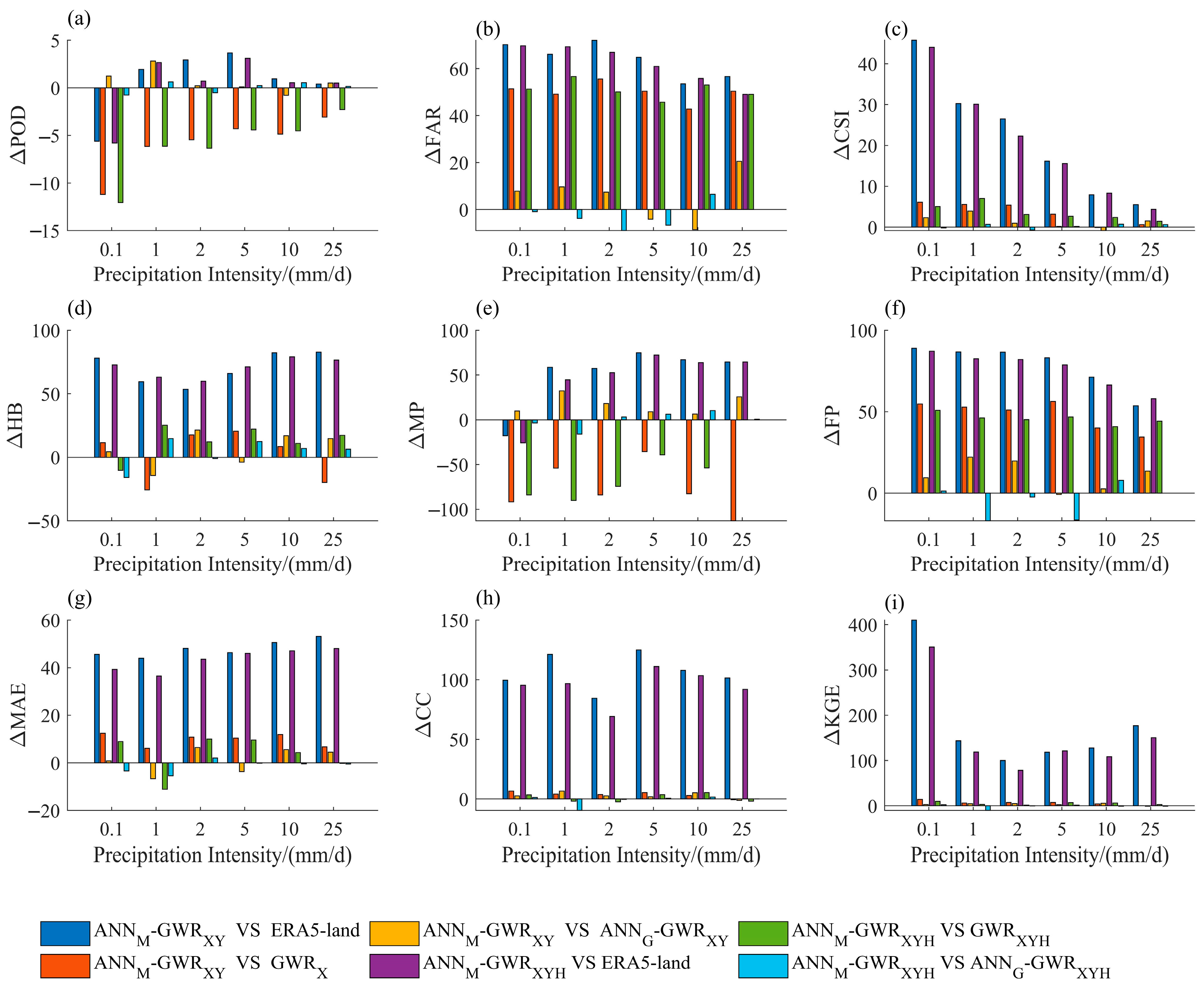
4.3. Model Gains Across Different Precipitation Intensities

Precipitation intensity was divided into six categories: (1) 0.1 mm/d ≤ P < 1 mm/d; (2) 1 mm/d ≤ P < 2 mm/d; (3) 2 mm/d ≤ P < 5 mm/d; (4) 5 mm/d ≤ P < 10 mm/d; (5) 10 mm/d ≤ P < 25 mm/d; and (6) P ≥ 25 mm/d.

Figure 7 presents the median estimation accuracy of daily precipitation across various intensity levels for six precipitation fusion schemes. The findings indicate that in the classification indices, the probability of detection (POD) increases with the intensity of precipitation. However, the ANN–GWR model consistently yields lower POD values than the GWR model, with the gap between the two models narrowing as precipitation intensity increases. The false alarm ratio (FAR) decreases as precipitation intensity rises, with the FAR for the ANN–GWR model being only 50% of that for the GWR model. The critical success index (CSI) also improves with increased precipitation intensity, showing a slight enhancement for the ANN–GWR model compared to the GWR model. When total bias (TB) is decomposed into hit bias (HB), missed precipitation (MP), and false precipitation (FP), no distinct pattern emerges across schemes for HB due to the offsetting of positive and negative values in the time series, although a general trend of increasing HB with higher precipitation intensity is observed. Due to the limitations of the post-fusion correction method, the ANN–GWR model’s MP is about 0.8 mm higher than that of the GWR model, while its FP is about 1.5 mm lower.

For quantitative indices, the mean absolute error (MAE), correlation coefficient (CC), and Kling–Gupta efficiency (KGE) all increase with precipitation intensity. Notably, the ANN–GWR model demonstrates a significant advantage over the GWR model in terms of MAE as precipitation intensity increases. However, for higher precipitation intensities, the ANN–GWR model underperforms compared to the GWR model in terms of CC and KGE, likely due to difficulties in accurately predicting the magnitude of heavy rainfall after fusion, leading to predictions of high-intensity rainfall as low-intensity events.

Figure 8 illustrates the median gains in estimation accuracy for different precipitation intensities according to various precipitation fusion gain schemes. The results show that, for quantitative indices, as precipitation intensity increases, the gains in both △CSI and △CSI decrease, following the general trend of diminishing returns as the amount of information decreases. In the case of △POD, although the relationships between different gain evaluation schemes are complex, the absolute value of the gain tends to decrease as precipitation intensity increases. The gains in △HB remain relatively stable across different precipitation intensities; however, it is important to note that, at lower precipitation intensities, the comparison between the GWR and ANN–GWR models may exhibit a negative gain of around −20%. The patterns in △FP are generally similar to those in POD, but for medium-intensity precipitation, scheme ➅ may show a negative gain.

For quantitative indices, in precipitation events with intensities above 2 mm/d, △MAE shows positive gains, with improvements of about 10% relative to the GWR model. However, for △CC and △KGE, there is almost no gain when comparing the GWR and ANN–GWR models, consistent with the patterns observed in the full-year and seasonal gain analyses. Conversely, relative to reference precipitation, gains of around 80% and 100% are observed for △CC and △KGE, respectively, with KGE gains exceeding 300% at lower precipitation intensities.

5. Discussion

Challenges and future directions: Challenges persist in reconciling detection-completeness trade-offs, particularly for frequent low-intensity events. Future work should prioritize the following: Bayesian model averaging to harmonize ANN–GWR outputs; assimilation of radar nowcasting data for real-time correction; development of precipitation phase-aware classification algorithms.

6. Conclusions

This study developed a novel ANN–GWR fusion framework that synergized ANN-based precipitation classification with geographically weighted regression, achieving significant advancements in multi-source precipitation estimation. The key conclusions and implications are summarized as follows:

1. Hybrid framework outperforms conventional methods. The integration of ANN and GWR addressed critical limitations of conventional approaches. While GWR provided spatially explicit rainfall quantification, its linear regression structure struggled with precipitation event detection (FAR = 39%). The ANN module, leveraging nonlinear activation functions, improved heavy rainfall classification accuracy by 15% (CSI: 0.55 → 0.68), particularly during summer monsoons. This hybrid architecture reduced false precipitation estimates by 63% (43.1 → 16.2 mm/yr), demonstrating superior robustness in complex terrain.

2. Error correction enhances spatial consistency. Through IDW-based interpolation and systematic error decomposition, the framework mitigated spatial discontinuities caused by ANN–GWR mismatches. The fusion model achieved an 18% reduction in spatial error variance compared to GWR, with MAE decreasing by 12.4% (0.77 → 0.70 mm) across intensity thresholds. Notably, seasonal analysis revealed maximum accuracy gains in winter (CSI + 30%), where ANN effectively corrected snow-cover-induced satellite artifacts.

This research provides a transferable paradigm for merging machine learning with spatial statistics in hydrological modeling, advancing toward climate-resilient precipitation monitoring systems.

References

1. Libertino, A.; Sharma, A.; Lakshmi, V.; Claps, P. A global assessment of the timing of extreme rainfall from TRMM and GPM for improving hydrologic design. Environ. Res. Lett. 2016, 11, 054003. [Google Scholar] [CrossRef]
2. Tang, G.; Zeng, Z.; Ma, M.; Liu, R.; Wen, Y.; Hong, Y. Can near-real-time satellite precipitation products capture rainstorms and guide flood warning for the 2016 summer in South China? IEEE Geosci. Remote Sens. Lett. 2017, 14, 1208–1212. [Google Scholar] [CrossRef]
3. Fu, Y.; Xia, J.; Yuan, W.; Xu, B.; Wu, X.; Chen, Y.; Zhang, H. Assessment of multiple precipitation products over major river basins of China. Theor. Appl. Climatol. 2016, 123, 11–22. [Google Scholar] [CrossRef]
4. Pereira, P.; Oliva, M.; Misiune, I. Spatial interpolation of precipitation indexes in Sierra Nevada (Spain): Comparing the performance of some interpolation methods. Theor. Appl. Climatol. 2016, 126, 683–698. [Google Scholar] [CrossRef]
5. Antal, A.; Guerreiro, P.M.P.; Cheval, S. Comparison of spatial interpolation methods for estimating the precipitation distribution in Portugal. Theor. Appl. Climatol. 2021, 145, 1193–1206. [Google Scholar] [CrossRef]
6. Hou, A.Y.; Kakar, R.K.; Neeck, S.; Azarbarzin, A.A.; Kummerow, C.D.; Kojima, M.; Oki, R.; Nakamura, K.; Iguchi, T. The global precipitation measurement mission. Bull. Am. Meteorol. Soc. 2014, 95, 701–722. [Google Scholar] [CrossRef]
7. Prakash, S.; Mitra, A.K.; Pai, D.S.; AghaKouchak, A. From TRMM to GPM: How well can heavy rainfall be detected from space? Adv. Water Resour. 2016, 88, 1–7. [Google Scholar] [CrossRef]
8. Shawky, M.; Moussa, A.; Hassan, Q.K.; El-Sheimy, N. Performance assessment of sub-daily and daily precipitation estimates derived from GPM and GSMaP products over an arid environment. Remote Sens. 2019, 11, 2840. [Google Scholar] [CrossRef]
9. Mekonnen, K.; Melesse, A.M.; Woldesenbet, T.A. Spatial evaluation of satellite-retrieved extreme rainfall rates in the Upper Awash River Basin, Ethiopia. Atmos. Res. 2021, 249, 105297. [Google Scholar] [CrossRef]
10. Hayashi, Y.; Tebakari, T.; Hashimoto, A. A Comparison Between Global Satellite Mapping of Precipitation Data and High-Resolution Radar Data–A Case Study of Localized Torrential Rainfall over Japan. J. Disaster Res. 2021, 16, 786–793. [Google Scholar] [CrossRef]
11. Batista, F.F.; Rodrigues, D.T.; e Silva, C.M.S. Analysis of climatic extremes in the Parnaíba River Basin, Northeast Brazil, using GPM IMERG-V6 products. Weather. Clim. Extrem. 2024, 43, 100646. [Google Scholar] [CrossRef]
12. Wang, Q.J.; Schepen, A.; Robertson, D.E. Merging seasonal rainfall forecasts from multiple statistical models through Bayesian model averaging. J. Clim. 2012, 25, 5524–5537. [Google Scholar] [CrossRef]
13. Shen, Y.; Zhao, P.; Pan, Y.; Yu, J. A high spatiotemporal gauge-satellite merged precipitation analysis over China. J. Geophys. Res. Atmos. 2014, 119, 3063–3075. [Google Scholar] [CrossRef]
14. Sideris, I.V.; Gabella, M.; Erdin, R.; Germann, U. Real-time radar–rain-gauge merging using spatio-temporal co-kriging with external drift in the alpine terrain of Switzerland. Q. J. R. Meteorol. Soc. 2014, 140, 1097–1111. [Google Scholar] [CrossRef]
15. Huang, C.; Zheng, X.; Tait, A.; Dai, Y.; Yang, C.; Chen, Z.; Li, T.; Wang, Z. On using smoothing spline and residual correction to fuse rain gauge observations and remote sensing data. J. Hydrol. 2014, 508, 410–417. [Google Scholar] [CrossRef]
16. Wu, H.; Yang, Q.; Liu, J.; Wang, G. A spatiotemporal deep fusion model for merging satellite and gauge precipitation in China. J. Hydrol. 2020, 584, 124664. [Google Scholar] [CrossRef]
17. Chen, C.; He, M.; Chen, Q.; Zhang, J.; Li, Z.; Wang, Z.; Duan, Z. Triple collocation-based error estimation and data fusion of global gridded precipitation products over the Yangtze River basin. J. Hydrol. 2022, 605, 127307. [Google Scholar] [CrossRef]
18. Brunsdon, C.; Fotheringham, S.; Charlton, M. Geographically weighted regression. J. R. Stat. Soc. Ser. D (Stat.) 1998, 47, 431–443. [Google Scholar] [CrossRef]
19. Dahamsheh, A.; Aksoy, H. Markov chain-incorporated artificial neural network models for forecasting monthly precipitation in arid regions. Arab. J. Sci. Eng. 2014, 39, 2513–2524. [Google Scholar] [CrossRef]
20. Akbari Asanjan, A.; Yang, T.; Hsu, K.; Sorooshian, S.; Lin, J.; Peng, Q. Short-term precipitation forecast based on the PERSIANN system and LSTM recurrent neural networks. J. Geophys. Res. Atmos. 2018, 123, 12543–12563. [Google Scholar] [CrossRef]
21. Nishant, N.; Hobeichi, S.; Sherwood, S.; Abramowitz, G.; Shao, Y.; Bishop, C.; Pitman, A. Comparison of a novel machine learning approach with dynamical downscaling for Australian precipitation. Environ. Res. Lett. 2023, 18, 094006. [Google Scholar] [CrossRef]
22. Sadeghi, M.; Asanjan, A.A.; Faridzad, M.; Nguyen, P.; Hsu, K.; Sorooshian, S.; Braithwaite, D. PERSIANN-CNN: Precipitation estimation from remotely sensed information using artificial neural networks–convolutional neural networks. J. Hydrometeorol. 2019, 20, 2273–2289. [Google Scholar] [CrossRef]
23. Grazzini, F.; Craig, G.C.; Keil, C.; Antolini, G.; Pavan, V. Extreme precipitation events over northern Italy. Part I: A systematic classification with machine-learning techniques. Q. J. R. Meteorol. Soc. 2020, 146, 69–85. [Google Scholar] [CrossRef]
24. Sahoo, B.; Bhaskaran, P.K. Prediction of storm surge and coastal inundation using Artificial Neural Network–A case study for 1999 Odisha Super Cyclone. Weather. Clim. Extrem. 2019, 23, 100196. [Google Scholar] [CrossRef]
25. Luo, C.; Li, X.; Ye, Y. PFST-LSTM: A spatiotemporal LSTM model with pseudoflow prediction for precipitation nowcasting. IEEE J. Sel. Top. Appl. Earth Obs. Remote Sens. 2020, 14, 843–857. [Google Scholar] [CrossRef]
26. Boroughani, M.; Soltani, S.; Ghezelseflu, N.; Pazhouhan, I. A comparative assessment between artificial neural network, neuro-fuzzy, and support vector machine models in splash erosion modelling under simulation circumstances. Folia Oecologica 2022, 49, 23–34. [Google Scholar] [CrossRef]
27. Wang, J.; Wang, Y.; Li, C.; Li, Y.; Qi, H. Landslide susceptibility evaluation based on landslide classification and ANN-NFR modelling in the Three Gorges Reservoir area, China. Ecol. Indic. 2024, 160, 111920. [Google Scholar] [CrossRef]
28. Brunsdon, C.; Fotheringham, A.S.; Charlton, M.E. Geographically weighted regression: A method for exploring spatial nonstationarity. Geogr. Anal. 1996, 28, 281–298. [Google Scholar] [CrossRef]
29. Ding, M.; Shen, Z.; Huang, R.; Liu, Y.; Wu, H. Cross-Validation Methods for Multisource Precipitation Datasets over the Sparse-Gauge Region: Applicability and Uncertainty. J. Hydrometeorol. 2024, 25, 1135–1145. [Google Scholar] [CrossRef]
30. Tang, G.; Behrangi, A.; Long, D.; Li, C.; Hong, Y. Accounting for spatiotemporal errors of gauges: A critical step to evaluate gridded precipitation products. J. Hydrol. 2018, 559, 294–306. [Google Scholar] [CrossRef]
31. Yu, C.; Hu, D.; Liu, M.; Wang, S.; Di, Y. Spatio-temporal accuracy evaluation of three high-resolution satellite precipitation products in China area. Atmos. Res. 2020, 241, 104952. [Google Scholar] [CrossRef]
32. Tian, Y.; Peters-Lidard, C.D.; Eylander, J.B.; Joyce, R.J.; Huffman, G.J.; Adler, R.F.; Hsu, K.; Turk, F.J.; Garcia, M.; Zeng, J. Component analysis of errors in satellite-based precipitation estimates. J. Geophys. Res. Atmos. 2009, 114. [Google Scholar] [CrossRef]
33. Yong, B.; Chen, B.; Tian, Y.; Yu, Z.; Hong, Y. Error-component analysis of TRMM-based multi-satellite precipitation estimates over mainland China. Remote Sens. 2016, 8, 440. [Google Scholar] [CrossRef]
34. Vrugt, J.A. MODELAVG: A MATLAB toolbox for postprocessing of model ensembles. Dep. Civ. Environ. Eng. Univ. Calif. Irvine 2016, 4130. [Google Scholar]
Figure 1. Technical scheme.
Remotesensing 17 02610 g001
Figure 2. Geographical location of the study area.
Remotesensing 17 02610 g002
Figure 3. Spatial distribution of long-term overall detection rates at each gauge for different models (detection rate: the ratio of correctly identified cases to the total number of cases).
Remotesensing 17 02610 g003
Figure 4. Relationship between precipitation detection rate and month, as well as precipitation intensity.
Remotesensing 17 02610 g004
Figure 5. Relative performance of different gain evaluation schemes after normalization.
Remotesensing 17 02610 g005
Figure 6. Box plots of the gain in each evaluation scheme. (ai) respectively represent the gain assessment results of POD, FAR, CSI, HB, MP, FP, MAE, CC and KGE.
Remotesensing 17 02610 g006
Figure 7. Estimation accuracy of daily precipitation across different intensity levels using various precipitation fusion methods. (ai) respectively represent the POD, FAR, CSI, HB, MP, FP, MAE, CC, and KGE indicators.
Remotesensing 17 02610 g007
Figure 8. Accuracy gain of precipitation fusion scheme to estimate daily precipitation of different intensification/%. (ai) respectively represent the gains of the POD, FAR, CSI, HB, MP, FP, MAE, CC, and KGE indicators under different precipitation levels.
Remotesensing 17 02610 g008