Article

Evaluation and Improvement of Ocean Color Algorithms for Chlorophyll-a and Diffuse Attenuation Coefficients in the Arctic Shelf

by
Yubin Yao
1,
Tao Li
1,2,*,
Qing Xu
3,
Xiaogang Xing
4,
Xingyuan Zhu
1 and
Yubao Qiu
5
1
College of Oceanic and Atmospheric Sciences, Ocean University of China, Qingdao 266100, China
2
Frontier Science Center for Deep Ocean Multispheres and Earth System (FDOMES), Ocean University of China, Qingdao 266100, China
3
College of Marine Technology, Ocean University of China, Qingdao 266100, China
4
State Key Laboratory of Satellite Ocean Environment Dynamics (SOED), Second Institute of Oceanography (SIO), Ministry of Natural Resources, Hangzhou 310012, China
5
Aerospace Information Research Institute, Chinese Academy of Sciences, Beijing 100094, China
*
Author to whom correspondence should be addressed.
Remote Sens. 2025, 17(15), 2606; https://doi.org/10.3390/rs17152606 (registering DOI)
Submission received: 9 June 2025 / Revised: 9 July 2025 / Accepted: 17 July 2025 / Published: 27 July 2025

Abstract

Arctic shelf waters exhibit high optical variability due to terrestrial inputs and elevated colored dissolved organic matter (CDOM) concentrations, posing significant challenges for the accurate retrieval of chlorophyll-a (Chl-a) and downwelling diffuse attenuation coefficients ( Κ d ( λ ) ). These retrieval biases contribute to substantial uncertainties in estimates of primary productivity and upper-ocean heat flux in the Arctic Ocean. However, the performance and constraints of existing ocean color algorithms in Arctic shelf environments remain insufficiently characterized, particularly under seasonally variable and optically complex conditions. In this study, we present a systematic multi-year evaluation of commonly used empirical and semi-analytical ocean color algorithms across the western Arctic shelf, based on seven expeditions and 240 in situ observation stations. Building on these evaluations, regionally optimized retrieval schemes were developed to enhance algorithm performance under Arctic-specific bio-optical conditions. The proposed OCx-AS series for Chl-a and Κ d -DAS models for Κ d ( λ ) significantly reduce retrieval errors, achieving RMSE improvements of over 50% relative to global standard algorithms. Additionally, we introduce QAA-LS, a modified semi-analytical model specifically adapted for the Laptev Sea, which addresses the strong absorption effects of CDOM and corrects the significant overestimation observed in previous QAA versions.

1. Introduction

Accelerated Arctic warming in recent decades, driven largely by increased solar energy absorption, has resulted in a near-surface atmospheric temperature rise of approximately 3.1 °C—about three times the global average [1,2,3]. In response to this warming, multi-year sea ice has undergone marked thinning, while summer ice extent has declined by more than 12% per decade since the late 20th century [4]. Coupled Model Intercomparison Project Phase 6 (CMIP6) multi-model ensemble simulations point to a likely transition toward seasonally ice-minimum conditions in the Arctic Ocean around mid-century [5]. Reductions in sea ice coverage alter the structure of the coupled air–ice–ocean system, reinforcing positive feedback that elevate upper ocean thermal storage and amplify the surface albedo response [6,7,8].
The Arctic Monitoring and Assessment Programme (AMAP) report highlights the rapid transformation of Arctic climate conditions, significantly affecting both the ecosystem and community structures [2]. Diminished sea ice coverage not only enlarges habitats for phytoplankton but also extends their growth season, boosting net primary productivity by over 30% [9,10]. These ecological transitions, closely aligned with hydrographic variability, modify the upper ocean’s inherent optical properties (IOPs; [11]). Accurate assessments of phytoplankton biomass and solar radiation transmission are crucial for understanding the impacts on Arctic climate, as shortwave radiation affects temperature modeling and ecosystem dynamics [12,13].
Given the environmental constraints in the Arctic, real-time field observations remain challenging, making ocean color remote sensing a vital means for monitoring marine environments. However, significant obstacles, including sea ice presence, low solar elevation, and frequent cloud cover, complicate satellite-based retrievals [14,15]. Global ocean color algorithms, derived from datasets with less than 3% Arctic representation [16,17], struggle with the region’s bio-optical characteristics due to high CDOM concentrations, shallow waters, and optically complex Case II conditions [18,19]. Uncertainties in remote sensing data can stem from atmospheric correction, sensor calibration, or limitations of the bio-optical model. Some studies have shown that global algorithms seriously overestimate the concentration of chlorophyll-a (Chl-a) in the Arctic and considerable variations are observed among different algorithms, especially in Case II waters [18,19,20,21,22].
Optical data of the ocean’s surface have become one of the mature products of satellite remote sensing, accompanied by various algorithmic models describing radiant attenuation in water [23]. Like the Chl-a algorithms, the Κ d ( λ ) algorithms based on Chl-a principles overestimate the adaptive capacity of Arctic algae under persistently low irradiance conditions [24], and those based on IOPs underestimate the impact of subsurface phytoplankton accumulation in high-latitude regions [25].
In response, regional algorithms have emerged as a new solution for accurately retrieving Arctic bio-optical properties. Wang and Cota [26] proposed polynomial and linear versions of regional algorithms based on Western Arctic Ocean observations, while Lewis and Arrigo [27] developed a large dataset to analyze Arctic bio-optical characteristics and introduced the AO.emp algorithm. The use of regional algorithms has improved the accuracy of satellite retrieval to a certain extent, proving its potential for development.
Despite growing interest in polar ocean color monitoring, systematic performance evaluation of widely used retrieval algorithms in Arctic shelf waters remains limited, particularly under seasonally variable and CDOM-dominated conditions. This gap hinders the reliable estimation of Chl-a and Κ d ( λ ) , which are essential for assessing primary productivity and upper ocean heating in this rapidly changing region.
This study provides a comprehensive assessment of empirical and semi-analytical ocean color algorithms using multi-year Arctic expedition datasets. Based on observed bio-optical characteristics, we propose optimized regional algorithms—OCx-AS and Κ d -DAS to enhance the accuracy of Chl-a and Κ d ( λ ) retrievals. These adaptations reduce uncertainty in remote sensing-derived estimates of primary productivity and upper ocean heat, thereby strengthening observational capacity in this rapidly evolving region.

2. Materials and Methods
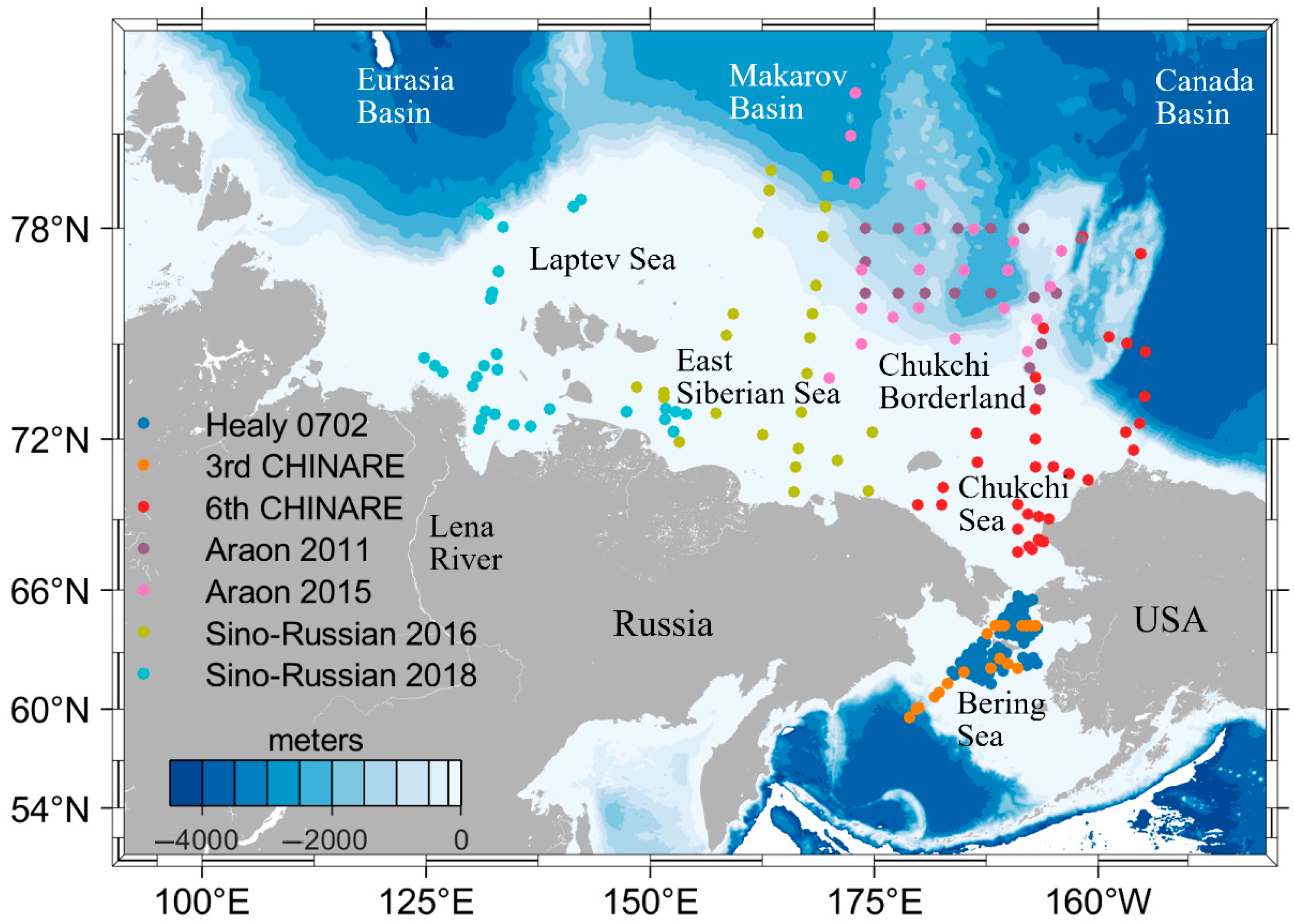
2.1. Study Area

This study focuses on the Western Arctic Ocean, encompassing the Bering Sea (BS), Chukchi Sea (CS), East Siberian Sea (ESS), and Laptev Sea (LS), as delineated in Figure 1. High primary productivity characterizes the BS and CS regions [28], which also function as gateways for northward transfer of thermal energy, freshwater, and biogeochemical constituents via the Bering Strait [29,30,31].
Occupying over 70% of the area, the continental shelves of the ESS and LS play a key role in regulating organic matter fluxes into the Arctic Ocean basin. Among the major contributors of terrestrial freshwater to the Arctic Ocean, the Lena River enters the Laptev Sea (73°N, 125°E), delivering a substantial load of CDOM and nutrients. The river begins to thaw in June, contributing a runoff volume of up to 541 k m 3 y e a r 1 to the LS [32]. Seasonal discharge from the Lena River contributes to the formation of the eastward-directed Siberian Coastal Current (SCC), which skirts the Siberian margin and enters the CS via the Long Strait, south of Wrangel Island. Here, it mixes with Pacific waters from the BS, forming the surface waters of the CS during summer, before deflecting offshore at the point where the pressure gradient vanishes [33,34].
Therefore, the hydrological characteristics of the shelf of the Western Arctic Ocean are primarily influenced by the terrestrial waters of the SCC and the marine waters from the Pacific. Semiletov et al. [35] defined a dynamic geochemical boundary (24.5 isohaline) in ESS to delineate the impacts of terrestrial and marine sources on the region. West of this boundary, hydrological properties are mainly affected by freshwater fluxes and coastal particle transport, while east of the boundary, the influence of Pacific-origin waters is more pronounced.

2.2. In Situ Data

This study incorporates hydrographic and bio-optical in situ observations acquired across 240 stations during seven Arctic research cruises conducted between 2007 and 2018 (station locations are illustrated in Figure 1 and Supplementary Material Section S1). The observational data in the ESS and LS were obtained during the Sino-Russian Arctic expeditions in 2016 and 2018, aboard the Russian research vessel “Akademik M.A. Lavrentyev”. The summer data for the BS and the CS were collected during the third (2008) and sixth (2014) Chinese National Arctic Research Expeditions (CHINARE), aboard the icebreaker “Xuelong”. Data in the spring of 2007 in the BS were obtained from the United States Coast Guard Cutter (USCGC), aboard the U.S. icebreaker “Healy”. The observational data in the Chukchi Borderland (CS_Borderland) were collected during the 2011 and 2015 Korean Arctic expeditions, aboard the research vessel “Araon”.
The optical observations in this study were conducted using the High-Resolution Profiling Reflectance Radiometer (PRR) system produced by Biosphere Sciences Inc., San Diego, USA. The PRR system comprises an underwater profiling radiometer, PRR-800, and a surface reference radiometer, PRR-810. The system operates at a sampling frequency of 10 Hz, with a bandwidth of 10 nm. The noise equivalent irradiance and radiance are 10−5 μWcm−2nm−1 and 10−6 μWcm−2nm−1sr−1, respectively. It measures light spectra across 18 wavelengths from 305 to 875 nm, with the visible light wavelengths utilized in this study including 380, 412, 443, 490, 510, 532, 555, 565, 589, 625, 665, 683, 710, 765, and 780 nm. The Κ d ( z , λ ) were derived from the profile-based optical observations, and the calculation follows Lambert–Beer’s law, which describes the exponential decay of downwelling irradiance with depth:
E d z = E d 0 e 0 z Κ d z , λ d z ,
where E d z is the downwelling irradiance at depth, E d 0 is the surface downwelling irradiance. The Κ d ( z , λ ) were determined by fitting a linear regression to the natural logarithm of irradiance within a specified depth range. Further details on the methodology can be found in Mueller et al. and Morel et al. [36,37].
Concurrent measurements of Chl-a concentration, seawater salinity, temperature, and turbidity were obtained using the ALEC CTD (Conductivity, Temperature, Depth profiler) system, manufactured by JFE Corporation, Nishinomiya, Japan. The temperature sensor has a detection range from −3 °C to 45 °C and the conductivity sensor’s range is from 2 to 70 mS/cm. The Chl-a sensor measures from 0 to 400 ppb (Uranine reference) with a resolution of 0.01 ppb. The fluorescence intensity of Chl-a (in ppb) was correlated with extracted Chl-a concentrations ( m g · m 3 or μg/L); the calibration curve can be checked in the Supplementary Material Section S2.

2.3. Satellite Data

This study employed remote sensing reflectance ( R r s ( λ ) ) data from MODIS-Aqua (Moderate Resolution Imaging Spectroradiometer) Level 3 products (4 km resolution, daily composites), accessed via the NASA (National Aeronautics and Space Administration; Greenbelt, MD, USA) Ocean Color portal (https://oceancolor.gsfc.nasa.gov/l3, accessed on 30 January 2025), and the selected wavelengths include 443, 488, 555, and 667 nm. The spectral bands used include R r s ( λ ) at 443, 488, 555, and 667 nm. This product employs a Multi-Band Atmospheric Correction (MBAC) scheme [38], which optimally utilizes additional spectral information provided by hyperspectral marine color sensors in the Shortwave Infrared and Near Infrared (NIR) bands. The R r s ( λ ) products primarily serve as inputs for Chl-a and Κ d ( λ ) algorithms, which are used to validate and compare with our optimized algorithms.

2.4. Ocean Color Algorithms

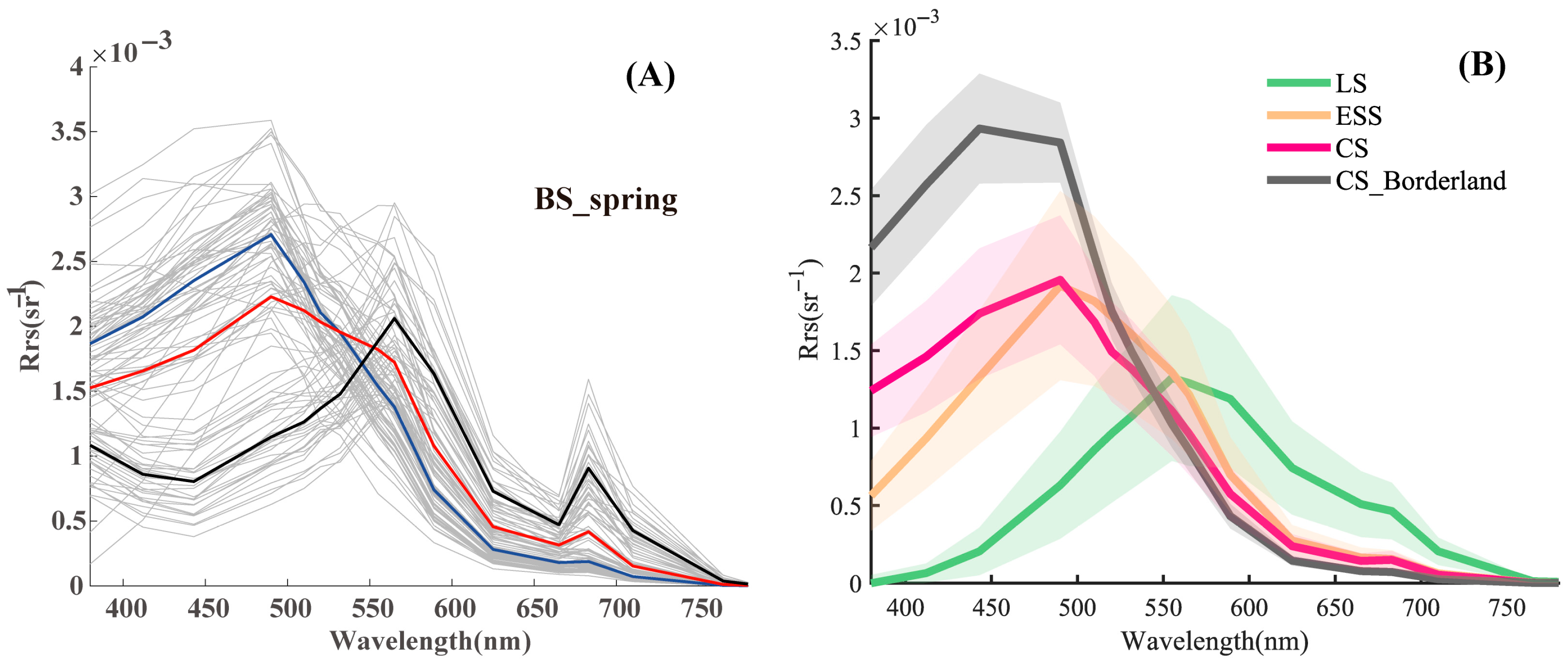
2.4.1. Remote Sensing Reflectance

Persistent sea ice coverage and frequent cloud contamination limited the valid matchup rate between in situ and satellite observations to below 10%, based on the spatiotemporal thresholds proposed by Bailey and Werdell [39]. As an alternative, we calculated R r s ( λ ) based on the measured upwelling radiance L u ( z ,   λ ) and downwelling irradiance E S ( 0 + ,   λ ) . The data were processed according to NASA’s optical observation standards [36], initially checking for anomalies in each profile’s E S ( 0 + ,   λ ) . To estimate the near-surface upwelling radiance L u ( 0 ,   λ ) , a linear regression was applied to the L u ( z ,   λ ) data obtained from the upper 6 m of each profile, achieving R 2 > 0.99. After correcting for instrument self-shadowing, the above-water radiance, L W ( 0 + ,   λ ) , was calculated using the air–sea interface transmission constant (0.543; [40]):
L W 0 + ,   λ = 0.543 × L u ( 0 ,   λ ) .
The spectral remote sensing reflectance R r s ( λ ) can be defined as the ratio of L W ( 0 + ,   λ ) to E S ( 0 + ,   λ ) :
R r s λ = L W 0 + ,   λ / E S ( 0 + ,   λ ) .

2.4.2. Chl-a Algorithms

I.
Blue–green ratio algorithm OCx (Ocean Color X)
The blue–green ratio algorithm (OCx, where x indicates the specific band configuration applied) is the primary empirical algorithm used in Chl-a remote sensing. OCx typically relies on the relationship between surface Chl-a concentration and the blue–green band ratio of R r s ( λ ) . The specific wavelengths for the blue–green ratio differ slightly among satellite sensors (Table 1), with blue light wavelengths approximately 443–532 nm and green light wavelengths around 551–560 nm. The standard algorithms adopted by MODIS, SeaWiFS (Sea-viewing Wide Field-of-view Sensor), and MERIS (Magneto-Electric Resonant Ionospheric Tomography) are based on fourth-order polynomial regressions applied to the maximum blue-to-green reflectance ratio (MBR):
C h l - a = 10 a 0 + a 1 R + a 2 R 2 + a 3 R 3 + a 4 R 4 ,
where R is the logarithm of the maximum blue–green ratio with base 10 ( log 10 ( M B R ) ), and a i ( i = 0 , 1 , 2 , , n ) are the fitted empirical or semi-empirical coefficients. The algorithm coefficients for SeaWiFS, MODIS, and MERIS primarily derive from observational datasets of Case I waters in mid- to low-latitude regions [17]. Initial Arctic-specific adaptations of OCx algorithms were developed using in situ datasets from marginal seas [22,26] and later refined by Lewis and Arrigo [27] into the AO.emp algorithm based on an expanded Arctic bio-optical database.
II.
Red light and NIR algorithms
Red light and NIR algorithms were initially applied to terrestrial vegetation remote sensing. With advancements in satellite sensor technology, studies have found that NIR bands exhibit notable responsiveness to Chl-a fluorescence in optically complex waters, enabling effective retrieval with reduced susceptibility to interference from non-algal particulates and CDOM [43]. Due to the shift in the absorption peak of Chl-a in NIR band with changes in Chl-a concentration [44], NIR algorithm design often starts by developing a band index (dual-band and triple-band) to test wavelength sensitivity, followed by calibrating empirical relationships linking the selected index to Chl-a. Commonly used NIR indices include the Ratio Vegetation Index (RVI, [45]), the Difference Vegetation Index (DVI), and the Normalized Difference Vegetation Index (NDVI), which combines band differences and ratios [46]:
R V I = R r s ( λ 2 ) / R r s ( λ 1 ) ,
D V I = R r s λ 2 R r s ( λ 1 ) ,
N D V I = [ R r s λ 2 R r s ( λ 1 ) ] / [ R r s λ 2 + R r s ( λ 1 ) ] ,
where λ 1 represents the red-light band where Chl-a strongly absorbs, while λ 2 is the NIR band where Chl-a strongly reflects.
In turbid waters, the presence of non-algal optical constituents reduces the robustness of dual-band algorithms. Dall’Olmo et al. [47] introduced a three-band algorithm (TBA), which utilizes a combination of a Chl-a absorption peak at λ 1 , a narrow Chl-a fluorescence peak at λ 2 , and a pure water absorption peak at λ 3 :
C h l - a [ ( R r s ( λ 1 ) R r s ( λ 2 ) ) ] R r s ( λ 3 ) ,
The absorption coefficients of yellow substances and inorganic suspended are approximately equal at λ 1 and λ 2 , allowing their effects to be subtracted by taking the difference. Because the backscattering coefficients at the three selected wavelengths are nearly equivalent, the TBA algorithm can partially suppress absorption effects from non-pigmented materials, making it suitable for use in moderately turbid waters.
Song et al. and Matsushita et al. [48,49], based on the principles of the TBA, developed the Three-Band Model (TBM) and the Maximum Chlorophyll Index (MCI) algorithms, respectively, to improve the detection of Chl-a in compositionally complex environments:
T B M = [ R r s λ 1 1 R r s λ 2 1 ] R r s ( λ 3 ) ,
M C I = R r s ( λ 2 ) R r s ( λ 1 ) [ λ 2 λ 1 λ 2 λ 1 ( R r s ( λ 3 ) R r s ( λ 1 ) ) ] ,
Finally, we also included the CI (Chlorophyll Index) algorithm in our evaluation system, which is used in conjunction with the OCx algorithm in satellite sensors. Although the CI algorithm is not strictly an NIR algorithm, it is designed to consider multiple wavelengths, including blue, green, and red light, serving as a case of multi-band integration. The CI algorithm is a three-band reflectance difference method that computes the deviation of green-band reflectance from a linear baseline constructed using blue and red bands [50]:
C I = R r s ( g ) [ R r s b + g b r b ( R r s ( r ) R r s ( b ) ) ] ,
where g , b , and r represent the green light, blue light, and red-light bands, respectively. Final calculation of CI Chl-a is carried out using two coefficients ( a 0 = 0.4287 , a 1 = 230.47 )
C h l - a = 10 a 0 + a 1 C I
Table 2 lists the NIR algorithms evaluated in this study.

2.4.3. Κ d λ Algorithms

I.
Direct Empirical Algorithms ( Κ d -Direct). The empirical algorithm is the primary method currently used by satellite sensors to retrieve Κ d ( 490 ) . The basic approach views Κ d ( 490 ) as composed of two components: Κ b i o ( 490 ) and Κ w ( 490 ) [54]. Κ b i o ( 490 ) refers to the total attenuation by biologically derived components, encompassing phytoplankton, associated microbes (e.g., viruses, bacteria), suspended particles, and CDOM:
Κ d 490 = Κ w 490 + Κ b i o 490 ,
where Κ w ( 490 ) is the Κ d ( λ ) for pure water at the 490 nm wavelength, with a value of 0.0166 m 1 . Κ d -Direct derives Κ b i o ( 490 ) from empirically calibrated ratios of blue to green R r s ( λ ) , and estimate Κ d ( 490 ) by using empirical model [55,56]:
Κ d ( 490 ) = 0.1660 + 10 a 0 + i = 1 4 a i ( log 10 ( R r s ( b ) R r s ( g ) ) i ) ,
The coefficients for each sensor’s algorithm are available from the NASA Ocean Color portal, as shown in Table 3.
II.
Indirect Empirical Algorithm ( Κ d -Indirect). Morel and Maritorena [54] assumed that regional attenuation is primarily influenced by phytoplankton along with co-varying contributions from yellow substances and non-algal materials. Under this framework, a power-law function is commonly used to approximate the link between Κ b i o λ and Chl-a. Thus, a two-step empirical model relating R r s ( λ ) , Chl-a, and Κ d ( λ ) can be constructed:
Κ b i o λ = X ( C h l - a ) e
The relationship between Chl-a and R r s ( λ ) has been established under the Chl-a algorithm scheme. At 490 nm, the coefficients—originally derived from mid- to low-latitude observations—take values of 0.0724 and 0.6896, respectively. Yao et al. [57], based on the in situ data of the Bering Sea, provided reference values of X and e as 0.1489 and 0.3805, respectively.
III.
Quasi-Analytical Algorithm (QAA). Quasi-analytical models are grounded in radiative transfer principles, linking the ocean’s apparent optical properties (AOPs) to its inherent optical properties (IOPs) and environmental boundary factors such as illumination geometry and surface conditions [58]. A crucial step in processing QAA is determining the absorption coefficient a ( λ ) and the backscattering coefficient b b ( λ ) from R r s ( λ ) . Once a ( λ ) and b b ( λ ) along with the boundary conditions are known, Κ d ( λ ) can be calculated from the quasi-analytical model [23,59]. The contributions of a ( λ ) and b b ( λ ) to attenuation are empirically quantified in the formula:
Κ d λ = m 0 a ( λ ) + m 1 ( 1 m 2 e m 3 a ( λ ) ) b b ( λ ) ,
where m 0 1 + 0.005 θ a , and θ a is the solar zenith angle. The parameters m 1 , m 2 , m 3 are 4.18, 0.52, and 10.8, respectively. When calculating the backscattering coefficient for pure water, reference values corresponding to the observed wavelengths are taken from Morel [60], and for wavelengths without direct observations, calculations are derived using Twardowski [61]. The model parameters remain constant across different waters and wavelengths, but a ( λ ) , b b ( λ ) , and boundary conditions require adjustments based on the study area.

2.5. Evaluation Criteria

We assessed algorithm accuracy and regional suitability using three statistical indicators: RMSE (Root Mean Square Error), MAE (Mean Absolute Error, also known as L1 norm), and MAPE (Mean Absolute Percentage Error). These metrics are defined as follows:
R M S E = 1 N i = 1 N ( m e a s u r e i e s t i m a t e i ) 2 .
M A E = 1 N i = 1 N e s t i m a t e i m e a s u r e i .
M A P E = 1 N i = 1 N e s t i m a t e i m e a s u r e i m e a s u r e i ( % ) .
The m e a s u r e i and e s t i m a t e i represent the measured and algorithm-derived values of the parameter, respectively, with N being the sample size.
For the results calculated by various algorithms, quartiles and the logarithmic ratios based on derived and measured values are good measures for assessing the dispersion of data:
W 1 , W 2 = [ Q 1 1.5 I Q R , Q 3 + 1.5 I Q R ] .
log_ratio = log ( e s t i m a t e i m e a s u r e i ) .
where Q 1 , Q 2 and Q 3 represent the 25%, 50%, and 75%, respectively, and the inter quartile range (IQR) defined as I Q R = Q 3 Q 1 . Finally, we employed a conventional linear regression model to assess the validity of the derived equations. Relevant statistical parameters include the coefficient of determination ( R 2 ), slope ( S ), intercept ( I ), and associated 95% uncertainty bounds.

3. Results

3.1. Chlorophyll a

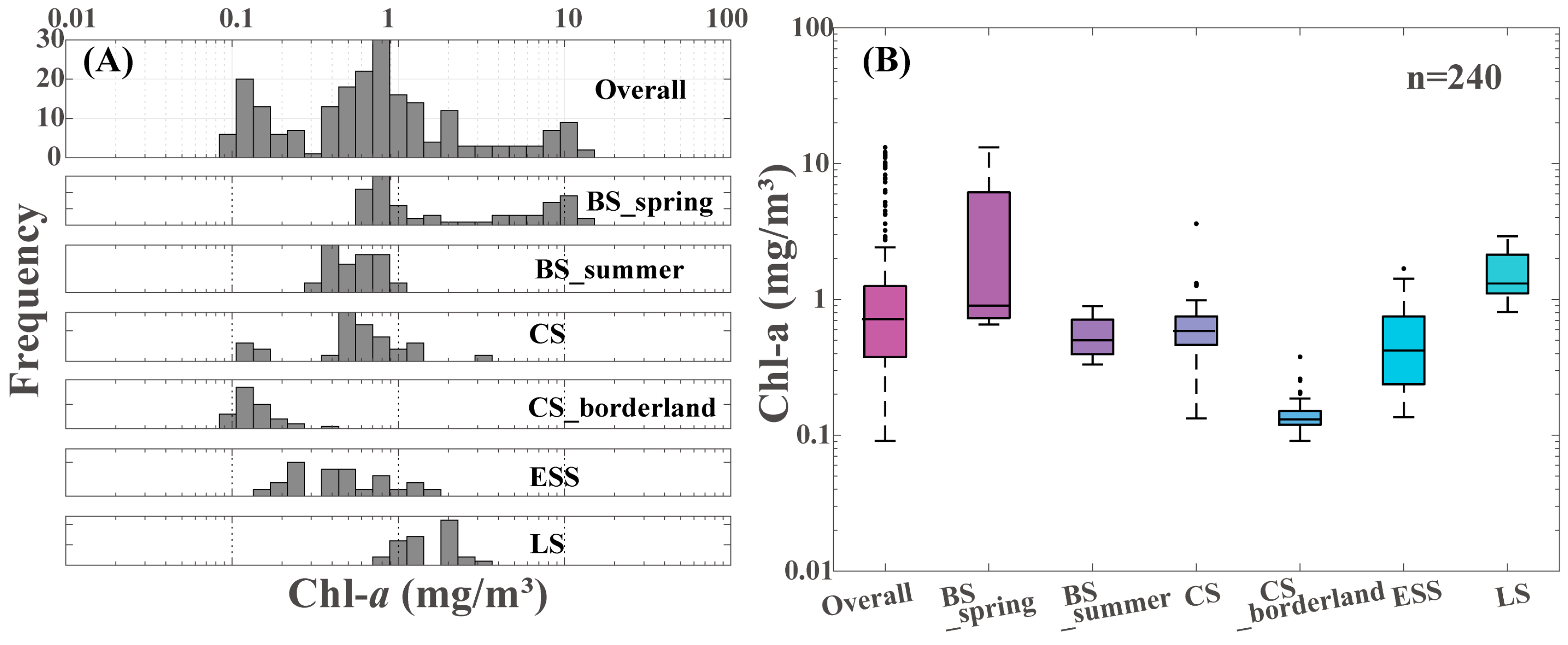
3.1.1. In Situ Observation of Chl-a Concentration

Satellite observations provide estimates of surface Chl-a concentrations. In this study, the calculations were conducted based on the ocean’s mixed layer depth, as shown in Table 4. Data from the CS_borderland was collected at the marginal ice zone. Zhao et al. [62] reported that the Subsurface Chlorophyll Maximum (SCM) in the Chukchi Borderland typically occurs between 30 and 60 m. As Chl-a concentrations above the SCM are relatively uniform, measurements from the upper 10 m are representative of near-surface conditions.
As illustrated in Figure 2, Chl-a concentrations most commonly fall between 0.35 and 2.30 m g · m 3 in all stations, while the summer Chl-a concentration is 1.63 ± 0.62 m g · m 3 on the LS, surpassing this range. This rise results from seasonal input from the Lena River, supplying substantial freshwater and nutrient loads to the marginal seas of the Arctic [63]. The average Chl-a concentration in the ESS and BS_summer are similar (0.56 ± 0.41 and 0.56 ± 0.19 m g · m 3 , respectively), but the compositions of their waters are markedly different. In the ESS, nutrient levels progressively decline as Laptev Sea waters are advected eastward following the northern Siberian margin [33,34,64]. These waters are characterized by complex optical components, including a significant presence of suspended particles and CDOM, which influence R r s ( λ ) . BS_summer reflects the consumption of remaining nutrients following the spring phytoplankton bloom [65], with water properties like Case I waters. As shown in Table 4, springtime in the BS features exceptionally elevated Chl-a levels (mean: 3.40 ± 3.88 m g · m 3 , with peaks above 13 m g · m 3 ), making it a valuable subset for testing algorithm performance in high-biomass conditions. Chl-a remains low (<0.68 m g · m 3 ) in BS_summer, CS, and CS_Borderland, reflecting the nutrient-poor conditions typical of polar waters.

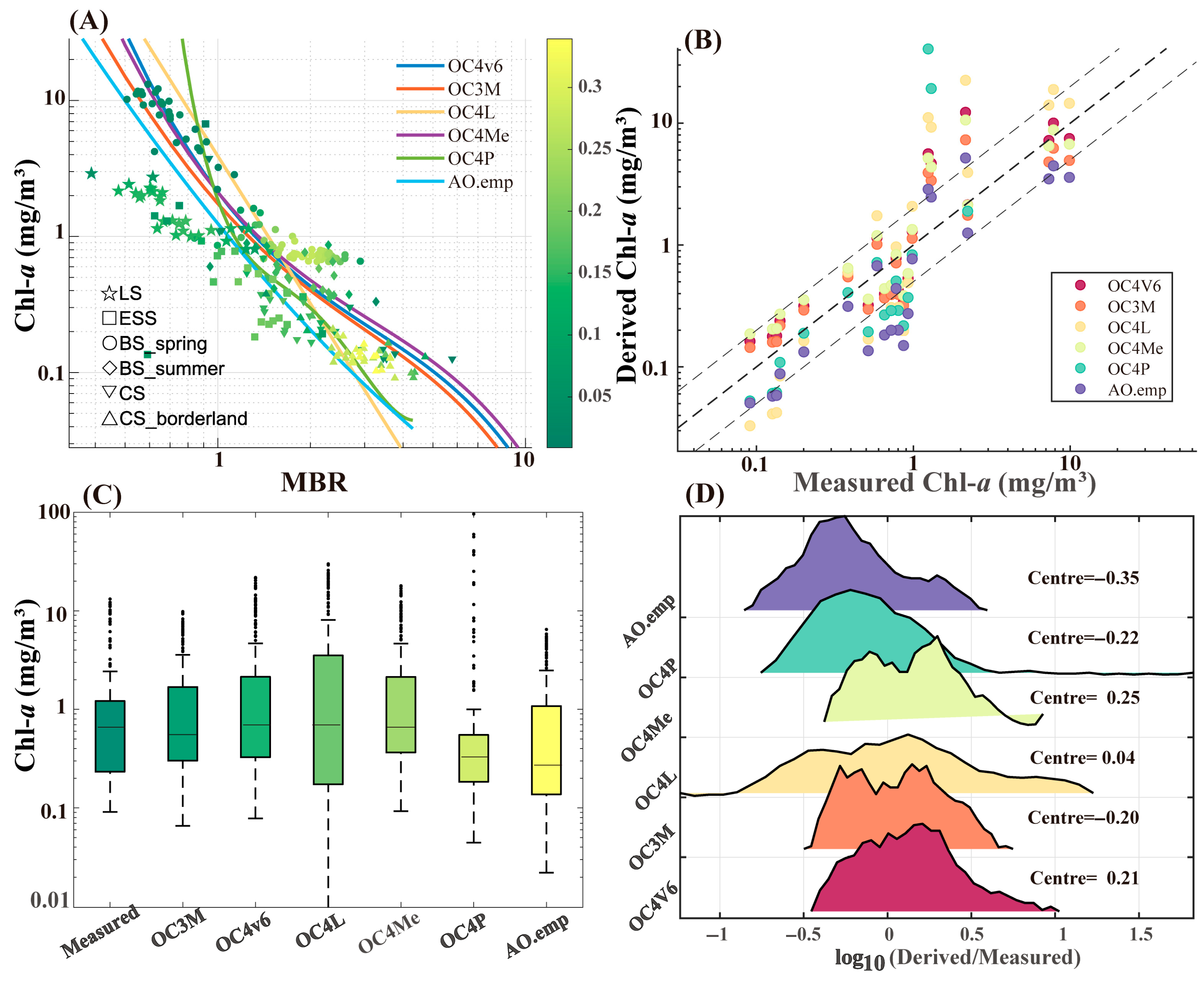
3.1.2. Evaluation of OCx Algorithms

Based on the extrapolated R r s ( λ ) , we employed six different OCx algorithms to derive the Chl-a concentration of the upper ocean and compared them with in situ measurements. The results indicate that the global algorithms from three satellite sensors (OC4v6, OC3M, OC4Me) and two Arctic regional algorithms (OC4L, OC4P) generally overestimate Chl-a concentration in the Arctic shelf, as shown in Figure 3A,B, with overestimation coefficients ranging from 1.68 to 2.92 (Table 5). Only the AO.emp algorithm showed a marked underestimation, with retrieved values averaging 1.02 ± 1.53 m g · m 3 and being 0.87 times the in situ measurements. Empirical algorithm performance varied by region, with the strongest fit observed in the BS_spring, where in situ measurements aligned closely with algorithm estimates (the correlation between Chl-a and Κ d ( λ ) exceeded 0.74; [57]). Under these conditions, which approximate Case I optical properties, global algorithms yielded reliable Chl-a retrievals at concentrations exceeding 1.0 m g · m 3 . Some stations in LS and ESS also recorded Chl-a > 1 m g · m 3 but the results from the MBR curves were significantly higher than observed values. Drozdova [66] reported surface DOC concentration at the Lena River mouth ranging from 242.5 to 886.7 μ m with a g ( λ ) at 350 nm, ranging from 2.36 to 11.17 m 1 . Such elevated CDOM levels can significantly bias Chl-a retrievals upward in this region [67,68]. For other stations characterized as typical polar low-nutrient waters, the derived values from the algorithms were generally overestimated, but the absolute errors were relatively smaller compared to regions with Chl-a > 1.0 m g · m 3 .
Among the evaluated algorithms, AO.emp demonstrated superior performance based on statistical metrics (RMSE = 1.69, MAPE = 59.8%). Nevertheless, it exhibits clear limitations—underestimating Chl-a concentrations in spring and overestimating them in summer, as illustrated in Figure 3A. Among global algorithms, OC3M showed the highest mean accuracy, producing an average concentration of 1.66 ± 2.71 m g · m 3 —well aligned with in situ observations. However, its retrieval errors were larger than those of AO.emp, with an RMSE of 1.76 and a MAPE of 76.4%. The broader spread of log errors for OC3M, shown in Figure 3D, further reflects this variability. The other regional algorithms, OC4L and OC4P, did not perform as well as expected, with RMSEs of 5.84 and 10.56, respectively, which are higher than those of the three global OCx algorithms. As shown in the box plot (Figure 3C), the medians of the three global algorithms (0.61, 0.55, 0.66 m g · m 3 ) are similar to that of OC4L (0.60 m g · m 3 ), but the estimates derived from OC4L exhibit a wider range of variation and greater dispersion. In contrast, the OC4P group is narrower due to an excess of outliers exceeding 1.5 IQR. This pattern is consistent with the distribution of log errors shown in Figure 3D.
Although the OC4P algorithm shows a favorable log-error center at 0.04, its error distribution shows a significantly flatter peak compared to other algorithms, indicating greater variability in its retrievals. Additionally, the standard deviations of the regional algorithms are greater than 6.91, and MAPE exceeds 171%, also indicating that the results estimated by OC4L and OC4P are more prone to outliers (Table 6). The suboptimal results from the two regional algorithms may stem from their limited calibration range, particularly for Chl-a concentrations below 0.6 m g · m 3 [26]. Figure 3A visualizes the differences between regional and global algorithms. As shown, the curves for OC4v6, OC3M, and OC4Me are very similar, and the divergence gradually increases as the MBR decreases from 1.0. The OC4P algorithm curve is too steep, resulting in severe overestimations when MBR is < 0.7 (Chl-a > 100 m g · m 3 , which accounts for 17% of OC4P’s results), and in the range of 0.7 < MBR < 1.0, results of OC4P also cause greater errors than other algorithms. Assessing regional algorithms within a limited range of Chl-a concentration might produce better results, but it would not fully reflect the optical characteristics of the Arctic shelf.

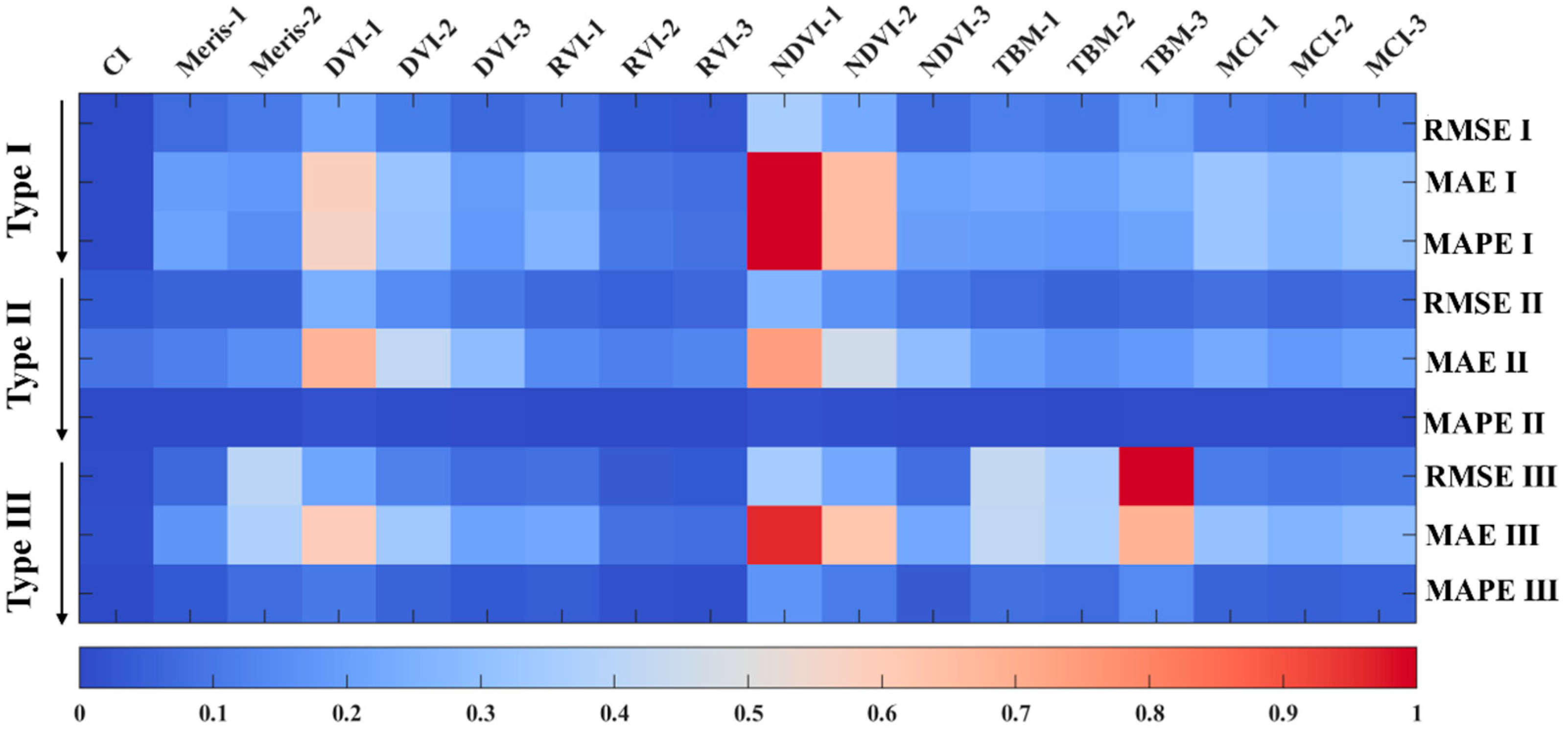
3.1.3. Evaluation of NIR Algorithms

Since Chl-a concentration alone is insufficient to evaluate NIR algorithm performance in the Arctic, we assess the R r s ( λ ) spectral behavior to determine the relative strength of red and NIR reflectance signals. The summer R r s ( λ ) spectra of various marginal seas, as shown in Figure 4B, display peak in the blue light band (443–490 nm) for CS and ESS and in the green light band at 565 nm for LS, with the largest variations in spectrum occurring around these peaks (corresponding to the areas of the shaded regions), and all regions show no significant peaks in the NIR band ( λ > 625 nm). The spectrum observed in the BS differs markedly from its summer counterpart (Figure 4A), with several stations exhibiting pronounced features in the longer wavelengths, particularly within the red and NIR regions. Based on the characteristics of R r s ( λ ) peaks, we categorize the spring R r s ( λ ) spectrum of the BS into three types: Type I, with a peak at 490 nm and no significant sub-peak in the red band; Type II, with a peak at 565 nm and a significant sub-peak in the red band; and Type III, with a peak in the blue–green band (443–565 nm) but no sub-peak or only a weak sub-peak.
There are significant differences in Chl-a concentrations among the different types, with average concentrations for Type I, II, III being 0.88 ± 0.32, 8.50 ± 2.58, and 2.10 ± 2.02 m g · m 3 , respectively. These are defined as low, high, and medium nutrient waters in the polar region, with their proportions in the BS_spring being 47:32:13. According to this classification, the summer LS belongs to Type III, while the other regions’ R r s ( λ ) spectra are Type I. Based on the R r s ( λ ) categories, we evaluated the applicability of common NIR and mixed algorithm CI in the Arctic shelf. Since there are significant differences in Chl-a concentrations among Type I, II, and III waters, we focus primarily on the MAPE when comparing the performance of algorithms. Evaluation results of the NIR algorithms, as shown in Table 7 and Figure 5 (a normalized statistical heatmap), indicate that the NIR algorithms perform best in Type II waters, with MAPE ranging from 90.5 to 796.1%. In contrast, the MAPE for Type I and III waters can reach 10 4 , indicating significant uncertainty when NIR algorithms are applied to Type I and III waters. Therefore, the discussion below primarily focuses on Type II waters.
Among the evaluation results, the CI algorithm performs closest to the observed Chl-a concentration (MAPE II = 90.5%). However, the CI is special in this section because the algorithm involves bands that include both blue–green light (443 and 555 nm) and red light (665 nm), making it impossible to quantify the contribution of red light separately. Apart from the CI algorithm, NIR algorithms can be broadly categorized into two-band and three-band algorithms. Among them, RVI-POW and TBM-POW exhibit the most notable performance in their respective categories, with MAPE II remaining below 180%. MAPE II results (176.7–258.0%) indicate that TBM and MCI yield similar performance across Arctic shelf waters. However, three-band algorithms demonstrate reduced adaptability relative to their two-band counterparts, as evidenced by the statistics in Table 7. Three-band index is approximated as [ R r s 1 665 R r s 1 709 ] × R r s ( 754 ) [ a p h 665 + a w 665 a p h 709 a w 709 ] / a w 754 ]   [49] where R r s ( 754 ) in low-nutrient environments like the Arctic is affected by pure water absorption, hindering detection of a strong signal (as shown in Figure 4). This effect constrains the effectiveness of three-band algorithms in such conditions.
Among empirical algorithms (L, POW, POL), the linear regression model exhibits worse suitability. The estimated values derived from linear regression for RVI and NDVI show greater variability and uncertainty compared to those obtained using the POW and POL regression models. We re-fitted and optimized the NIR-based algorithms, significantly reducing RMSE (see Supplementary Material Section S3 for detail). However, their performance remains far inferior to the OCx-AS algorithm, making them unsuitable for Arctic remote sensing.

3.2. Diffuse Attenuation Coefficients

3.2.1. In Situ Observation of Κ d ( λ )

As shown in Figure 6A, the remarkable attenuation in red light and ultraviolet light ( λ < 412   n m ) has presented with the low attenuation in blue–green light within spectral range of 313–683 nm. The red light is mainly absorbed by surface pure water, while the absorption of ultraviolet light is contributed by CDOM [61,69]. There are obvious differences in radiation attenuation between terrestrial and marine sources waters. Yao et al. [57] reported that the Κ d ( 490 ) in the Bering Sea during spring exceed those in summer, but these levels are only comparable to those of ESS, respectively, at 0.20 ± 0.19 and 0.15 ± 0.10 m 1 (Table 8). The ESS waters represent a dilution and freshening process as they are transported along the SCC from LS. The attenuation magnitude of LS is much higher than other areas in the study region, with Κ d ( 490 ) in the summer LS being 6.4 times that of the BS_summer, indicating that terrestrial runoff inputs have a significant impact on radiation attenuation. The Κ d ( 490 ) of BS and CS in summer are closely matched (0.08 ± 0.05 and 0.09 ± 0.05 m 1 , respectively), both reflecting the characteristics of Pacific waters. Progressive nutrient loss during Pacific water transport results in lower nutrient levels at CS_Borderland compared to other regions, yielding the minimum Κ d ( 490 ) observed—just 0.05 ± 0.02 m 1 .
Since the Κ d ( λ ) at 490 nm is an important parameter in applications, we analyzed its frequency distribution in the Arctic Shelf. As shown in Figure 6B, the main range of Κ d ( 490 ) is concentrated between 0.03 and 0.12 m 1 (frequency > 10), defining 0.1 m 1 as the boundary between medium and low values for the study area. Clearly, the medium–high value areas are mainly distributed in the BS_spring, ESS, and LS, while the attenuation of marine source waters in summer is primarily concentrated in the medium–low value areas. Compared with the Chl-a frequency distribution in Figure 2A, elevated Chl-a concentrations are linked to stronger light attenuation, suggesting that regions influenced by marine source waters experience greater attenuation as biomass increases. However, despite having lower Chl-a concentrations than those observed in BS_spring, terrestrial source waters exhibit greater attenuation. This indicates that, beyond pigments, other optically active constituents significantly contribute to the attenuation of radiation in water bodies. Morel et al. [37] also found that the contribution of pigment to increasing attenuation is limited: in Case I waters, Κ d ( 490 ) is likely to exceed 0.5 m 1 only at Chl-a approaching 20 m g · m 3 . In the LS region, however, Κ d ( 490 ) are 0.51 ± 0.24 m 1 as the Chl-a is only 1.68 ± 0.70 m g · m 3 .

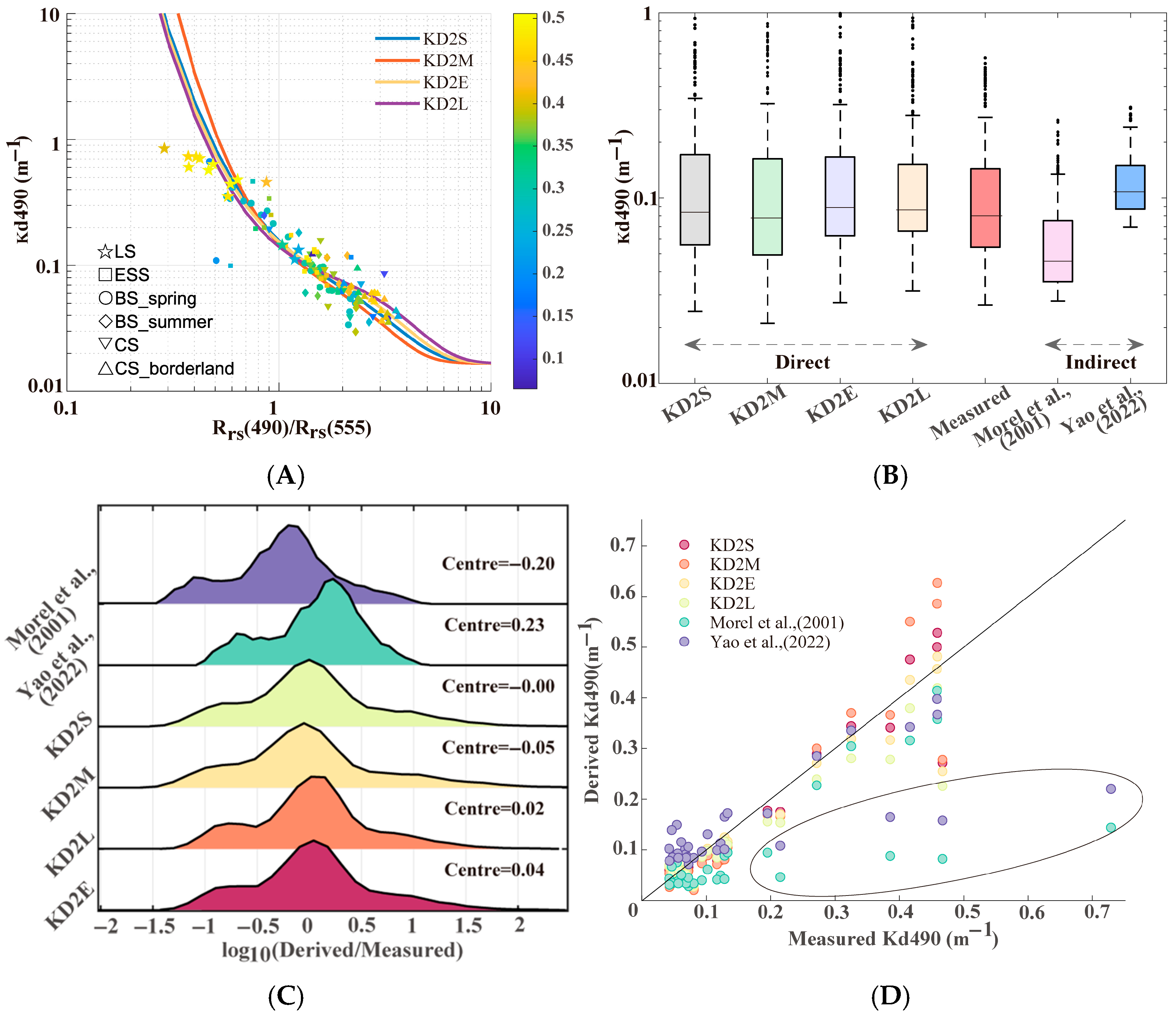
3.2.2. Evaluation of the Empirical Algorithms for Κ d ( λ )

Unlike the evaluation of OCx algorithms, Κ d -Direct lacks regional algorithms widely used in the Arctic. In addition, it is no longer necessary to calculate the MBR because the attenuation of the waters must comprehensively consider the influence of all optical components. Figure 7A illustrates how the Κ d -Direct algorithms relate to the blue-to-green reflectance ratio.
The evaluation results of Κ d -Direct exhibit a high agreement with the measured values. However, the algorithm slightly overestimates the overall regional Κ d 490 , with KD2S, KD2E, and KD2L performing similarly (average overestimation factors from 1.16 to 1.20; Table 9), and KD2M showing relatively larger errors (average overestimation factor at 1.36). The distribution of measured data primarily concentrates on two different ranges, namely, Κ d 490 < 0.1 m 1 and Κ d 490 close to 1.0 m 1 , reflecting the attenuation characteristics of marine and terrestrial source waters. Marine source waters are characterized by an elevated blue–green ratio and a reduced Κ d 490 , while terrestrial source waters exhibit the opposite trend. Among all evaluated Κ d -Direct algorithms, KD2L performs most prominently with an average Κ d 490 of 0.18 ± 0.24 m 1 very close to the actual measurement of 0.18 ± 0.20 m 1 while both RMSE and MAE are at 0.12 and 0.05, the smallest among the evaluated algorithms, respectively (Table 10). Additionally, the MODIS sensor, which performs best in Chl-a algorithms (OC3M), generates the greatest uncertainty when retrieving Κ d ( 490 ) with an RMSE of 0.36, nearly double that of other algorithms. Meanwhile, the estimated value of KD2M shows the largest variation range (Figure 7B), responding to the most dramatic changes in the blue–green ratio.
To evaluate the performance of Κ d -Indirect, we examined the Κ d -Indirect algorithms proposed by Morel and Maritorena [54] and Yao et al. [57]. As depicted in Figure 7B, the results of the Κ d -Indirect are very close to the median of the observations, but the two Κ d -Indirect algorithms show starkly different outcomes. Yao et al.’s results are characterized by overestimation (RMSE = 0.15, MAE = 0.08), while Morel et al.’s results show underestimation (RMSE = 0.17, MAE = 0.09). The frequency distribution in Figure 7C indicates that the core of Κ d -Direct is centered near 0, suggesting that most results of the algorithm are close to observed values. However, the core frequencies of Κ d -Indirect are centered around 0.0 ± 0.2. The MAPE values of Κ d -Indirect (43.7 and 57.1%) are higher than all Κ d -Direct algorithms, indicating that the results of the Κ d -Indirect are significantly affected by outliers. Combined with Figure 7D, it is obvious that the KD2M deviates significantly from the measured value in the waters of high attenuation. And the response of Κ d -Indirect to high attenuation will show two signals, due to the flaws of the Κ d -Indirect (it attributes the causes of high attenuation solely to chlorophyll, leading to outliers in LS and ESS, as shown in the circles in Figure 7D). Overall, KD2L demonstrates superior performance among the evaluated empirical algorithms, while KD2M’s strong response to the blue–green ratio tends to produce outliers. Κ d -Indirect algorithms will fail to reflect the comprehensive optical characteristics of the Arctic shelf if only the contribution from the chlorophyll in the radiation attenuation is considered. Additionally, a preliminary evaluation of a Κ d 490 model based on L w λ was also conducted, but showed poor performance compared to R r s λ -based approaches. Details are provided in the Supplementary Material Section S4.

3.2.3. Evaluation of the QAA Algorithms

The essence of the empirical algorithm for retrieving Κ d ( λ ) is the process of inferring AOP from Chl-a, while QAA algorithms derive AOPs from IOPs, both using R r s ( λ ) as the initial values. All datasets from this study were input into the classical QAA model for evaluation of the results, revealing significant errors in the high attenuation range ( Κ d 490 > 0.1 m 1 ) with an RMSE exceeding 2.97. Further analysis of the isolated LS subset revealed that its unique optical features were the primary contributors to the observed errors (Figure 8). The QAA model exhibits excellent performance in retrieving Κ d 490 for BS, CS, and ESS (Table 11), with RMSE (0.11) and MAE (0.05) slightly better than the best-performing empirical algorithm KD2L, indicating that the QAA achieves the lowest absolute errors. However, the MAPE (39.7%) is higher than that of Κ d -Direct, indicating fewer stable variations between algorithmic results and measured values, particularly in the regions of lower Κ d 490 . As shown in Figure 8A, we found that the relative error of the QAA significantly decreases with increasing Κ d 490 when applied to the Arctic shelf, with the maximum error being 80%, and the in situ observations being primarily concentrated in the Κ d 490 < 0.1 m 1 . Despite larger relative errors in low-attenuation regions, the small values of Κ d 490 limit their contribution to the algorithm’s overall absolute error. Therefore, the QAA algorithm is highly applicable to BS, CS, and ESS.
The classical QAA algorithm applied to the LS showed severe overestimation, accompanied by substantial uncertainty, with all statistical values significantly exceeding those of other algorithms (MAPE = 373.5%), while the relative error for Κ d 490 can reach up to 1718%. The reason is that the a 555 band is still influenced by Chl-a and CDOM (Lee et al., [59]) in waters with high absorption rates, resulting in an incorrect a 555 based on the empirical formula with the blue–green ratio. Therefore, the classical QAA algorithm needs to be optimized and improved when applied to a region like LS.

4. Discussion

4.1. Improvement of Algorithms

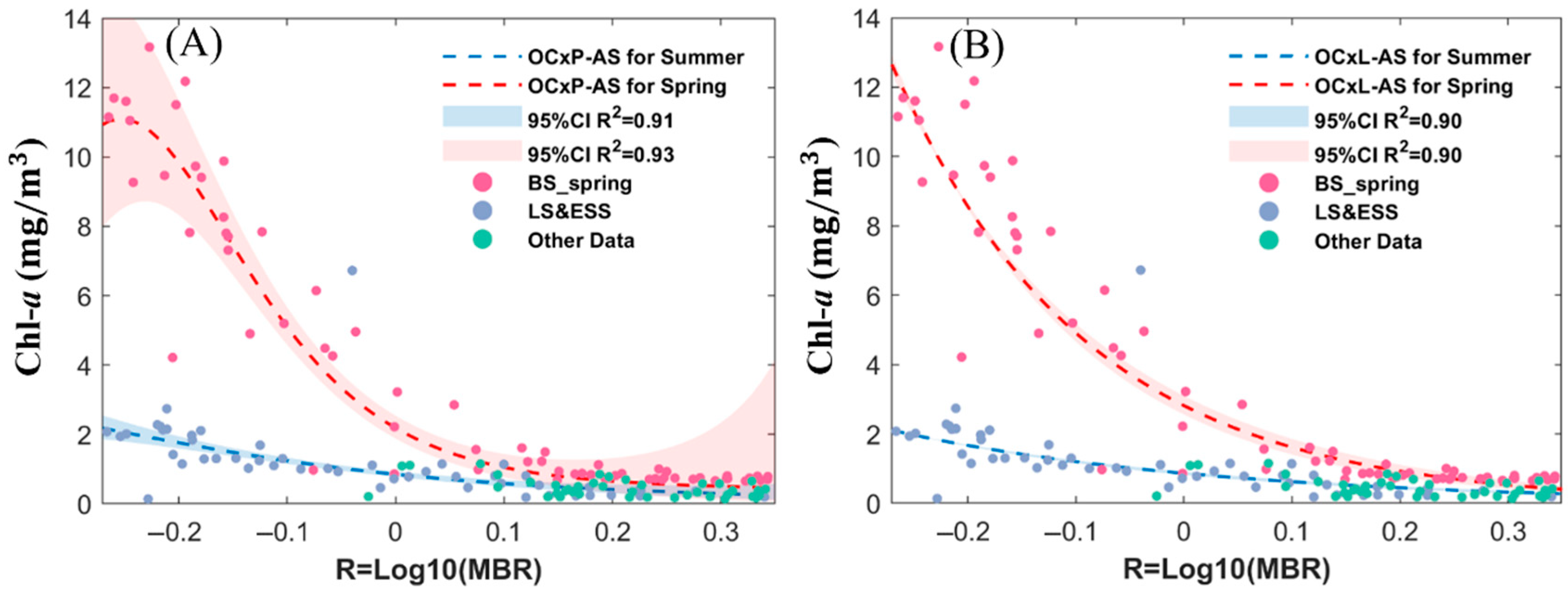
4.1.1. OCx Algorithms

The evaluation results indicate that existing OCx algorithms struggle to accurately retrieve sea surface Chl-a concentrations in the Arctic shelf. Therefore, we developed a new regional algorithm—OCx-AS (OCx-Arctic Shelf)—informed by in situ measurements. As illustrated in Figure 3A, the relationship between MBR and elevated Chl-a concentrations differs noticeably between spring and summer, showing two distinct seasonal patterns. Applying a single algorithm across both spring and summer introduces notable biases, typically underestimating Chl-a during spring and overestimating it in summer, as seen with AO.emp. Meanwhile, Figure 9 shows that when R exceeds 0.1, its association with Chl-a becomes more consistent and tightly clustered. Based on this observation, BS_summer and CS data (green points) were used as the foundation, and BS_spring data (red points), as well as the combined LS and ESS data (blue points), were separately incorporated into the fitting process (OCx-AS). This approach ensures that the characteristics of phytoplankton blooms are highlighted in spring and the bio-optical differences between terrestrial and marine sources are distinguished in summer.
Figure 9A shows the curves fitted in the polynomial format along with scatter plots of observed Chl-a concentrations. Notably, Chl-a concentrations are elevated in spring compared to summer under equivalent R conditions. The new seasonal algorithms yield R 2 of 0.93 and 0.91 (parameters in Table 12), marking a substantial improvement over previous models (RMSE of 0.81 and 0.21, respectively), and enabling more accurate Chl-a estimation across the region. To compare the merits of the OCxL-AS and OCxP-AS, we also present the new algorithm in the linear format. Figure 9B illustrates that the fit of the linear format in spring demonstrates poorer performance with scatter points compared to OCxP-AS. Specifically, the R 2 value decreases from 0.93 to 0.90, while the corresponding spring RMSE increases to 0.90. These results highlight the superior performance of OCxP-AS during the spring season.
There seems like no difference between the OCxL and OCxP format in summer ( R 2 and RMSE are close). In fact, the OCxP and OCxL have their own characteristics: The OCxP-AS curve is constrained by the measured Chl-a concentrations, ensuring that estimated values do not deviate from reality. However, it may lead to underestimations in high Chl-a concentration areas; The OCxL format has a narrower confidence interval and lower uncertainty, making its algorithm curve more aggressive in retrieving high Chl-a concentrations, particularly suitable in coastal areas. The difference between OCxL and OCxP format mainly lies in the degree of the polynomial. Attempts to change the degree for fitting algorithm parameters show a slight improvement in R 2 (e.g., from 0.93 to 0.94 in spring for OCxP). Considering the universality of the fourth power, we retain it as the final version. Cota et al. [22] also mentioned that although higher-order polynomial relationships can slightly improve statistical fitting results, they are not always recommended because the potential biological and physical principles of complex non-linear models are difficult to understand. Additionally, we calculated the fitting results in different functional forms and none performed as well as the OCx did.

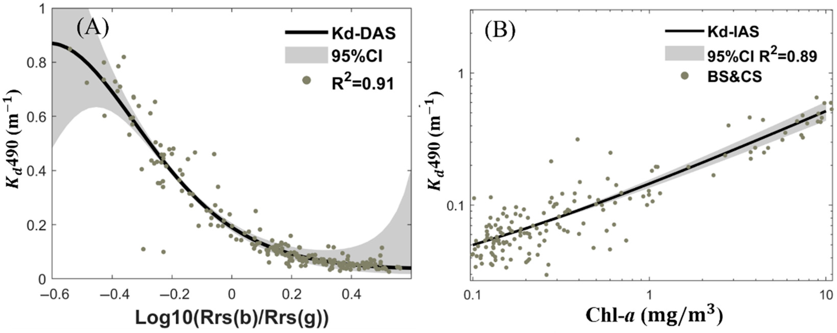
4.1.2. Empirical Algorithms for Κ d ( λ )

To improve the accuracy of satellite-derived surface Κ d 490 , new parameter algorithms ( Κ d -DAS and Κ d -IAS) for both Κ d -Direct and Κ d -Indirect were proposed based on measured data from the Arctic shelf (Figure 10; Table 13). There is a high consistency between the measured data and the Κ d -DAS with a reduced uncertainty ( R 2 = 0.91, RMSE = 0.06), representing an improvement of over 50% in RMSE compared to the previous algorithms. Confidence interval of 95% in Figure 10A revealed that the uncertainty significantly increases at log 10 ( R r s ( b ) / R r s ( g ) ) < 0.24 and log 10 ( R r s ( b ) / R r s ( g ) ) > 0 , corresponding to Κ d 490 > 0.5 m 1 and Κ d 490 < 0.2 m 1 . The sources of error in Κ d -DAS primarily arise from two aspects: (1) although the Κ d -Direct shows superiority over Κ d -Indirect in retrieving high attenuation waters, R r s ( b ) / R r s ( g ) still mainly reflects changes in chlorophyll, making it difficult to fully retrieve the attenuation conditions of Case II waters; (2) the Κ d λ is still an AOP that is influenced by the local light field. Furthermore, we introduced an improved version of the Κ d -Indirect algorithm tailored for marine water bodies, termed Κ d -IAS (Figure 10B). Performance evaluation in BS and CS demonstrated its strong applicability ( R 2 = 0.89, RMSE = 0.05), with a relatively stable 95% confidence interval width as Chl-a concentration increases. Compared to the existing Κ d -Indirect algorithms, the newly introduced parameters exhibit a significant improvement.
Both Κ d -DAS and Κ d -IAS showed robust adaptability in marine source water. The design of Κ d -Indirect algorithm constrains its effectiveness beyond Type I waters, making Κ d -DAS the more generalizable solution.

4.1.3. QAA Algorithms for LS

In QAA Version 4, Lee et al. [70] proposed using the 640 nm band as the reference wavelength for high-absorption waters instead of 555 nm, as a w 640 is five times greater than a w 555 . This reduces the proportion of absorption attributed to optically active substances relative to total absorption. The performance evaluation (Figure 11A and Table 14) showed that QAAV4 tends to underestimate Κ d 490 (0.36 ± 0.28 m 1 ), with an RMSE of 0.3044—nearly ten times smaller than that of the classical QAA—and notable improvements across other statistical metrics. However, a substantial proportion of the computed R r s ( 640 ) values from QAAV4 exhibited anomalies (Figure 11B), introducing biases in the estimation of a ( 640 ) . The latest version, QAA Version 6 [71], introduced R r s ( 670 ) to refine the estimation of a ( 555 ) . Nevertheless, when applied to LS, QAAV6 produced significantly overestimated results. With Κ d 490 = 1.43 ± 0.80 m 1 , QAAV6’s statistical performance (RMSE = 1.10) was inferior to QAAV4.
Building upon previous QAA versions, we developed the QAA-LS algorithm, specifically designed to accommodate the unique optical characteristics of LS (Table 15). The primary modification involves introducing a new calculation formula for R r s ( 640 ) (Step 1). The power function-derived R r s ( 640 ) was used as a reference value for linear regression analysis against the Step 1 output, yielding R 2 > 0.99 (Figure 11A). This improvement effectively solves the problem of anomalies in R r s ( 640 ) computation (Figure 11B).
Unlike QAAV4, QAA-LS employs 640 nm as the reference band; QAA-LS retains 555 nm for calculations. The R r s ( λ ) spectrum of LS suggests the feasibility of a red–green ratio, while Lee [59] previously attempted to establish a relationship between a ( 555 ) and R r s 640 for high-absorption waters (Step 2). As shown in Figure 11C, the QAA-LS-derived a ( 555 ) values are more concentrated, a ( 555 ) = 0.18 ± 0.07 m 1 , whereas the QAAV6-derived values are more dispersed ( a ( 555 ) = 0.46 ± 0.24 m 1 ).
The QAA-LS-estimated Κ d 490 is 0.62 ± 0.33 m 1 , approximately 1.24 times the measured value (Table 14), demonstrating superior performance in LS compared to all existing QAA versions. Statistical metrics show significant improvements over QAAV4 and QAAV6, with reductions in RMSE (0.19) and MAE (0.15), corresponding to an improvement of 36% in RMSE compared to QAAV4. The relative difference between model outputs and in situ observations spans from 3% to 85%. Across the entire range of Κ d 490 , the estimated values exhibit strong consistency with the measured data and are no longer constrained by the magnitude of attenuation (Figure 12D).
Since the in situ data available for the LS was relatively limited, we conducted a sensitivity analysis by perturbing R r s ( λ ) at input wavelengths (490, 555, and 665 nm) by ±5% to further demonstrate its robustness. The resulting changes in estimated Κ d 490 and the sensitivity index ( S i ) are summarized in Table 16. The Κ d 490 variations were generally within ±1.2% for ±5% R r s ( λ ) perturbations at 490 nm (−1.05% for +5% and −1.16% for −5%), indicating a relatively low sensitivity at this wavelength and a stable inverse response. Perturbations at 555 nm resulted in even smaller Κ d 490 changes (∼0.18–0.19%), while perturbations at 665 nm led to modest increases (∼0.7%). These results demonstrate that the QAA-LS algorithm exhibits robust performance, with output Κ d 490 showing limited sensitivity to realistic R r s ( λ ) uncertainties. The consistently low S i values further confirm QAA-LS’s superiority in retrieving radiative attenuation in the LS.

4.2. Retrieval Scheme

4.2.1. Chl-a Retrieval Scheme for Arctic Shelf

Due to the limitation of nutrient conditions in the Arctic Ocean, the comprehensive performance of NIR algorithms is significantly inferior to that of the OCx algorithms. While the CI algorithm leverages information from the blue, green, and red bands, its performance on the Arctic shelf remains inferior to that of OCx-based approaches. NASA and NOAA typically combine CI with OCx in their operational Chl-a products [50,72] to enhance global applicability. However, the evaluation results (Table 7) have shown that the CI algorithm does not reduce the retrieval uncertainty in the Arctic, suggesting that blue and green bands remain the more reliable choice for this region.
Through an overall assessment of empirical Chl-a algorithms, our recommended approach is to use the OCxP-AS algorithm in spring and the OCxL-AS in summer. Using updated parameters, the two OCx-AS algorithms reduced RMSE values from 1.69 to 0.81 and 0.22, reflecting over 52% improvement and confirming their effectiveness in Arctic marginal seas. To visualize the changes with the OCx-AS algorithms, we compared them with several years of satellite remote sensing products. Among the evaluation results, the Chl-a concentration derived from AO.emp was shown to be closest to the measured data. Accordingly, we applied MODIS-Aqua R r s ( λ ) products from 2013 to 2023 to estimate the Chl-a concentration and evaluated their consistency against outputs from the AO.emp algorithm. It should be noted that, as atmospheric correction schemes were not considered, the Chl-a concentrations estimated in this manner are not the final product outputs, and we are more interested in the relative differences between the two algorithms. Figure 12 shows that OCx-AS algorithms yield reduced summer Chl-a estimates relative to AO.emp (Figure 12A,B), aligning with the evaluation result in Table 6, while the differences in spring are less significant (Figure 12C,D).
Although integrating Arctic-specific bio-optical data has improved OCx algorithm accuracy, the substantial spatial and seasonal heterogeneity across Arctic waters precludes treating them as a single optical regime. The lack of nutrients in the Arctic Ocean surface during summer [73] may cause OCx algorithms to overestimate Chl-a when relying solely on the MBR signal. As seen in Figure 12B, especially in coastal areas such as the Lena River Delta and Norton Sound, terrestrial runoff causes excessively sharp gradients in Chl-a concentrations because the OCx algorithms cannot separate various optical components from the MBR signal, mistakenly classifying them as pigment. In fact, high concentrations of CDOM in these estuaries have been confirmed [66,74].
Coachman [33] identified clear contrasts in water properties between the Anadyr Water (AW) in the western Bering Sea and the Alaska Coastal Water (ACW) to the east. AW and ACW exhibit contrasting thermohaline and nutrient profiles—AW is characterized by colder, saltier, and nutrient-enriched conditions, whereas ACW tends to be warmer, fresher, and nutrient-depleted. The Chl-a distribution retrieved by AO.emp blurs the characteristics of these water masses, showing uniformly consistent Chl-a concentrations across the shelf (Figure 12D), while OCxL-AS clearly displays the nutrient distribution differences between the east and west (Figure 12C).

4.2.2. Κ d λ Retrieval Scheme for Arctic Shelf

The evaluation results of the empirical Κ d ( λ ) algorithms demonstrate that Κ d -DAS has stronger adaptability in the Arctic shelf, both in Case I waters and in the optically complex LS. Compared to Chl-a algorithms, Κ d -Direct offers less physical interpretability because it establishes relationships with all optically effective substances in the region without the need to quantify individual contributions. The QAA model, based on radiative transfer models and IOPs, offers strong physical interpretability, but variations in optical components may introduce errors in the calculation of IOPs ( a ( λ ) , b b p ( λ ) ). These errors can accumulate and lead to significant deviation in Κ d ( λ ) . We note that the QAA algorithm performs excellently in study areas other than LS because of the high proportion of absorption by non-phytoplankton substances at short wavelengths in the LS. Through optimization, we gradually reduced the uncertainty of the QAA in the Arctic Ocean, successfully lowering the MAPE to 29.2% and proving the potential for QAA development. However, the statistical results of QAA perform worse than Κ d -DAS. Since the QAA requires longer computation times and more input, we suggest that the Κ d -Direct is more suitable for the Arctic shelf.
Based on satellite R r s ( λ ) products, we compared the estimated values of Κ d -DAS with those of KD2L, verifying the application of Κ d -Direct-AO (Figure 13). Since Landsat 8 lacks a directly applicable R r s ( λ ) product, we still used the R r s ( λ ) products of MODIS from August 2013 to 2023 for estimation, which did not affect our results because we do not focus on the absolute values of Κ d ( 490 ) in this section. The results of Κ d -DAS are very close to those of KD2L, with the main differences in coastal areas, as KD2L did not account for the specificity of areas and underestimated the impact of terrestrial runoff. On this basis, the proposed Κ d -DAS algorithm effectively enhances the performance of the Κ d -Direct algorithms in the Arctic Ocean, making it the most suitable option for retrieving regional shortwave attenuation properties.

5. Conclusions

Accurate retrieval of Chl-a and Κ d ( λ ) is critical for understanding primary productivity and upper ocean thermodynamics in Arctic shelf waters, where global algorithms often fail due to complex optical conditions. In practice, space agencies commonly input the same initial marine signals (irradiance and reflectance) into various algorithms, integrating outputs under certain conditions. The uncertainty in the final products may be linked to the atmospheric correction approaches, sensor calibration, or the uncertainties of the algorithms. Our work specifically quantifies the errors generated by the ocean color algorithms.
The results demonstrate that the marginal seas cannot be uniformly classified as Case I waters. BS and CS, influenced by Pacific waters, exhibit optical characteristics dominated by chlorophyll absorption, while LS and ESS, significantly impacted by runoff, display strong contributions from non-algal materials, resembling Case II waters. Global Chl-a algorithms designed for Case I waters struggle in the Arctic shelf, while NIR algorithms exhibit even more inferior performance. For Κ d ( λ ) retrieval, Κ d -Direct algorithms demonstrate superiority in the optically complex Arctic Shelf. In contrast, Κ d -Indirect algorithms cannot get rid of non-algal material contributions in terrestrial waters.
Our findings emphasize the importance of adapting retrieval algorithms to the distinct bio-optical features of Arctic environments. The proposed optimized schemes—OCx-AS, Κ d -DAS, and QAA-LS—address these challenges and provide practical tools for improving the reliability of satellite-based Arctic marine monitoring.
Looking ahead, further refinement of bio-optical models that integrate additional environmental variables, such as CDOM absorption dynamics and subsurface phytoplankton distribution, could enhance the performance of retrieval algorithms. Continued accumulation of in situ measurements will also be essential for improving the accuracy of remote sensing products and supporting long-term ecological assessments under ongoing Arctic climate change.

Supplementary Materials

The following supporting information can be downloaded at: https://www.mdpi.com/article/10.3390/rs17152606/s1, Section S1. Station Information; Section S2. Correction of Chl-a concentration; Section S3. Improvement of NIR Algorithms; Section S4. Evaluation of a Κ d ( 490 ) model derived from L w ( λ ) . References [75,76,77] are cited in the Supplementary Materials.

Author Contributions

Software, X.Z.; Writing—original draft, Y.Y.; Writing—review & editing, Y.Y., Q.X., X.X. and Y.Q.; Project administration, T.L. All authors have read and agreed to the published version of the manuscript.

Funding

This study was supported by the National Key Research and Development Program of China (2021YFC2801204 and 2022ZD0117201) and the National Natural Science Foundation of China (42276239 and T2261149752).

Data Availability Statement

The original contributions presented in this study are included in the article/Supplementary Materials. Further inquiries can be directed to the corresponding author.

Acknowledgments

We are deeply grateful to the organizers, crews and scientists involved in the seven expeditions that made this research possible. Special appreciation goes to the data collectors Zhao Jinping, Jiao Yutian, and Lee W. Cooper (Healy-0702); Zhuang Yanpei (3rd CHINARE); Hao Qiang (6th CHINARE); Eun Jin Yang (Araon—2011, 2015); Wang Xiaoyu, Hu Limin (Sino-Russian 2016); Liu Yilin and Wu Yanjun (Sino-Russian 2018) for their invaluable contributions.

Conflicts of Interest

The authors declare no conflict of interest.

Nomenclature

SymbolDescriptionUnit
a ( λ ) Absorption coefficient of the total m 1
a g ( λ ) Absorption coefficient of colored dissolved organic matter (CDOM) and detritus m 1
a w ( λ ) Absorption coefficient for pure water m 1
b b ( λ ) Backscattering coefficient of the total m 1
b b p ( λ ) Backscattering coefficient of suspended particles m 1
b b w ( λ ) Backscattering coefficient of pure water m 1
Chl-aConcentration of chlorophyll-a m g · m 3
L w ( λ ) Water-leaving radiance W c m 2 n m 1 s r 1
n L w ( λ ) Normalized Water-leaving radiance W c m 2 n m 1 s r 1
L u ( λ ) Upwelling radiance W c m 2 n m 1 s r 1
E d ( λ ) Downwelling irradiance μ W c m 2 n m 1
  E s ( λ ) Downwelling irradiance just below the surface μ W c m 2 n m 1
Κ d ( λ ) Downwelling diffuse attenuation coefficient m 1
R r s ( λ ) Above-surface remote-sensing reflections s r 1
r r s ( λ ) Below-surface remote-sensing reflections s r 1

References

  1. Sledd, A.; L’Ecuyer, T.S. Emerging trends in Arctic solar absorption. Geophys. Res. Lett. 2021, 48, e2021GL095813. [Google Scholar] [CrossRef] [PubMed]
  2. AMAP. Impacts of Short-Lived Climate Forcers on Arctic Climate, Air Quality, and Human Health; Arctic Monitoring and Assessment Programme (AMAP): Tromsø, Norway, 2021. [Google Scholar]
  3. IPCC. Climate Change 2014 Synthesis Report; Intergovernmental Panel on Climate Change (IPCC): Geneva, Switzerland, 2014. [Google Scholar]
  4. Stroeve, J.C.; Kattsov, V.; Barrett, A.; Serreze, M.; Pavlova, T.; Holland, M.; Meier, W.N. Trends in Arctic sea ice extent from CMIP5, CMIP3 and observations. Geophys. Res. Lett. 2012, 39, L16502. [Google Scholar] [CrossRef]
  5. Zhao, H.; Li, J.; WANG, Z.; Wang, X. CMIP6 Simulations of the Arctic Sea Ice and Their Ensemble Projection of Ice-Free Time in Boreal Summer. Adv. Mar. Sci. 2024, 42, 238–253. [Google Scholar] [CrossRef]
  6. Perovich, D.K.; Light, B.; Eicken, H.; Jones, K.F.; Runciman, K.; Nghiem, S.V. Increasing solar heating of the Arctic Ocean and adjacent seas, 1979–2005: Attribution and role in the ice-albedo feedback. Geophys. Res. Lett. 2007, 34, L19505. [Google Scholar] [CrossRef]
  7. Shimada, K.; Kamoshida, T.; Itoh, M.; Nishino, S.; Carmack, E.; McLaughlin, F.; Zimmermann, S.; Proshutinsky, A. Pacific Ocean inflow: Influence on catastrophic reduction of sea ice cover in the Arctic Ocean. Geophys. Res. Lett. 2006, 33, L08605. [Google Scholar] [CrossRef]
  8. Arndt, S.; Nicolaus, M. Seasonal cycle of solar energy fluxes through Arctic Sea ice. Cryosphere Discuss 2014, 8, 2923–2956. [Google Scholar] [CrossRef]
  9. Arrigo, K.R.; Van Dijken, G.L. Secular trends in Arctic Ocean net primary production. J. Geophys. Res. Oceans 2011, 116, C09011. [Google Scholar] [CrossRef]
  10. Arrigo, K.R.; Van Dijken, G.L. Continued increases in Arctic Ocean primary production. Prog. Oceanogr. 2015, 136, 60–70. [Google Scholar] [CrossRef]
  11. Pavlov, A.K.; Stedmon, C.A.; Semushin, A.V.; Martma, T.; Ivanov, B.V.; Kowalczuk, P.; Granskog, M.A. Linkages between the circulation and distribution of dissolved organic matter in the White Sea, Arctic Ocean. Cont. Shelf Res. 2016, 119, 1–13. [Google Scholar] [CrossRef]
  12. Chen, J.; Zhang, X.; Xing, X.; Ishizaka, J.; Yu, Z. A Spectrally Selective Attenuation Mechanism-Based Kpar Algorithm for Biomass Heating Effect Simulation in the Open Ocean. J. Geophys. Res. Oceans 2017, 122, 9370–9386. [Google Scholar] [CrossRef]
  13. Ciavatta, S.; Brewin, R.; Skakala, J.; Sursham, D.; Ford, D. Assimilation of ocean colour to improve the simulation and understanding of the Northwest European shelf-sea ecosystem. In Proceedings of the EGU General Assembly Conference, Vienna, Austria, 23–28 April 2017; p. 18899. [Google Scholar]
  14. IOCCG. Ocean Colour Remote Sensing in Polar Seas; Babin, M., Arrigo, K., Bélanger, S., Forget, M.H., Eds.; International Ocean Colour Coordinating Group (IOCCG): Dartmouth, NS, Canada, 2015. [Google Scholar]
  15. Glukhovets, D.; Kopelevich, O.; Yushmanova, A.; Vazyulya, S.; Sheberstov, S.; Karalli, P.; Sahling, I. Evaluation of the CDOM absorption coefficient in the Arctic seas based on Sentinel-3 OLCI data. Remote Sens. 2020, 12, 3210. [Google Scholar] [CrossRef]
  16. O’Reilly, J.E.; Maritorena, S.; Siegel, D.A.; O Brien, M.C.; Toole, D.; Mitchell, B.G.; Kahru, M.; Chavez, F.P.; Strutton, P.; Cota, G.F. Ocean color chlorophyll a algorithm for SeaWiFS, OC2, and OC4: Version 4. SeaWiFS Postlaunch Calibration Valid. Anal. 2000, 11 Pt 3, 9–23. [Google Scholar]
  17. Werdell, P.J.; Bailey, S.W. An improved in-situ bio-optical data set for ocean color algorithm development and satellite data product validation. Remote Sens. Environ. 2005, 98, 122–140. [Google Scholar] [CrossRef]
  18. Vetrov, A.A.; Romankevich, E.A.; Belyaev, N.A. Chlorophyll, primary production, fluxes, and balance of organic carbon in the Laptev Sea. Geochem. Int. 2008, 46, 1055. [Google Scholar] [CrossRef]
  19. Morel, A.; Gentili, B.; Claustre, H.; Babin, M.; Bricaud, A.; Ras, J.; Tieche, F. Optical properties of the “clearest” natural waters. Limnol. Oceanogr. 2007, 52, 217–229. [Google Scholar] [CrossRef]
  20. Wang, M.; Shi, W. The NIR-SWIR combined atmospheric correction approach for MODIS ocean color data processing. Opt. Express 2007, 15, 15722–15733. [Google Scholar] [CrossRef]
  21. Mustapha, S.B.; Belanger, S.; Larouche, P. Evaluation of ocean color algorithms in the southeastern Beaufort Sea, Canadian Arctic: New parameterization using SeaWiFS, MODIS, and MERIS spectral bands. Can. J. Remote Sens. 2012, 38, 535–556. [Google Scholar] [CrossRef]
  22. Cota, G.F.; Wang, J.; Comiso, J.C. Transformation of global satellite chlorophyll retrievals with a regionally tuned algorithm. Remote Sens. Environ. 2004, 90, 373–377. [Google Scholar] [CrossRef]
  23. Lee, Z.; Darecki, M.; Carder, K.L.; Davis, C.O.; Stramski, D.; Rhea, W.J. Diffuse attenuation coefficient of downwelling irradiance: An evaluation of remote sensing methods. J. Geophys. Res. Oceans 2005, 110, C02017. [Google Scholar] [CrossRef]
  24. Brunelle, C.B.; Larouche, P.; Gosselin, M. Variability of phytoplankton light absorption in Canadian Arctic seas. J. Geophys. Res. Oceans 2012, 117, C00G17. [Google Scholar] [CrossRef]
  25. Xing, X.; Boss, E.; Zhang, J.; Chai, F. Evaluation of ocean color remote sensing algorithms for diffuse attenuation coefficients and optical depths with data collected on BGC-Argo floats. Remote Sens. 2020, 12, 2367. [Google Scholar] [CrossRef]
  26. Wang, J.; Cota, G.F. Remote-sensing reflectance in the Beaufort and Chukchi seas: Observations and models. Appl. Opt. 2003, 42, 2754–2765. [Google Scholar] [CrossRef]
  27. Lewis, K.M.; Arrigo, K.R. Ocean color algorithms for estimating chlorophyll a, CDOM absorption, and particle backscattering in the Arctic Ocean. J. Geophys. Res. Oceans 2020, 125, e2019JC015706. [Google Scholar] [CrossRef]
  28. Grebmeier, J.M. Shifting patterns of life in the Pacific Arctic and sub-Arctic seas. Annu. Rev. Mar. Sci. 2012, 4, 63–78. [Google Scholar] [CrossRef]
  29. Woodgate, R.A.; Weingartner, T.; Lindsay, R. The 2007 Bering Strait oceanic heat flux and anomalous Arctic sea-ice retreat. Geophys. Res. Lett. 2010, 37, L01602. [Google Scholar] [CrossRef]
  30. Serreze, M.C.; Francis, J.A. The Arctic amplification debate. Clim. Change 2006, 76, 241–264. [Google Scholar] [CrossRef]
  31. Walsh, J.J.; Dieterle, D.A.; Maslowski, W.; Grebmeier, J.M.; Whitledge, T.E.; Flint, M.; Sukhanova, I.N.; Bates, N.; Cota, G.F.; Stockwell, D. A numerical model of seasonal primary production within the Chukchi/Beaufort Seas. Deep Sea Res. Part II 2005, 52, 3541–3576. [Google Scholar] [CrossRef]
  32. Bauch, D.; Hölemann, J.; Willmes, S.; Gröger, M.; Novikhin, A.; Nikulina, A.; Kassens, H.; Timokhov, L. Changes in distribution of brine waters on the Laptev Sea shelf in 2007. J. Geophys. Res. Oceans 2010, 115, C11008. [Google Scholar] [CrossRef]
  33. Coachman, L.K.; Aagaard, K.; Tripp, R.B. Bering Strait: The Regional Physical Oceanography; University of Washington Press: Seattle, WA, USA, 1995. [Google Scholar]
  34. Weingartner, T.J.; Danielson, S.; Sasaki, Y.; Pavlov, V.; Kulakov, M. The Siberian Coastal Current: A wind-and buoyancy-forced Arctic coastal current. J. Geophys. Res. Oceans 1999, 104, 29697–29713. [Google Scholar] [CrossRef]
  35. Semiletov, I.; Dudarev, O.; Luchin, V.; Charkin, A.; Shin, K.H.; Tanaka, N. The East Siberian Sea as a transition zone between Pacific-derived waters and Arctic shelf waters. Geophys. Res. Lett. 2005, 32, L10614-1. [Google Scholar] [CrossRef]
  36. Mueller, J.L.; Morel, A.; Frouin, R.; Davis, C.; Voss, K. Ocean Optics Protocols for Satellite Ocean Color Sensor Validation, Revision 4; Goddard Space Flight Space Centre: Greenbelt, MD, USA, 2003; Volume 3, pp. 7–19. [Google Scholar] [CrossRef]
  37. Morel, A.; Huot, Y.; Gentili, B.; Werdell, P.J.; Hooker, S.B.; Franz, B.A. Examining the consistency of products derived from various ocean color sensors in open ocean (Case 1) waters in the perspective of a multi-sensor approach. Remote Sens. Environ. 2007, 111, 69–88. [Google Scholar] [CrossRef]
  38. Ibrahim, A.; Franz, B.A.; Ahmad, Z.; Bailey, S.W. Multiband atmospheric correction algorithm for ocean color retrievals. Front. Earth Sci. 2019, 7, 116. [Google Scholar] [CrossRef]
  39. Bailey, S.W.; Werdell, P.J. A multi-sensor approach for the on-orbit validation of ocean color satellite data products. Remote Sens. Environ. 2006, 102, 12–23. [Google Scholar] [CrossRef]
  40. Volpe, G.; Colella, S.; Brando, V.E.; Forneris, V.; La Padula, F.; Di Cicco, A.; Sammartino, M.; Bracaglia, M.; Artuso, F.; Santoleri, R. Mediterranean ocean colour Level 3 operational multi-sensor processing. Ocean Sci. 2019, 15, 127–146. [Google Scholar] [CrossRef]
  41. O’Reilly, J.E.; Maritorena, S.; Mitchell, B.G.; Siegel, D.A.; Carder, K.L.; Garver, S.A.; Kahru, M.; McClain, C. Ocean color chlorophyll algorithms for SeaWiFS. J. Geophys. Res. Oceans 1998, 103, 24937–24953. [Google Scholar] [CrossRef]
  42. O’Reilly, J.E.; Werdell, P.J. Chlorophyll algorithms for ocean color sensors-OC4, OC5 & OC6. Remote Sens. Environ. 2019, 229, 32–47. [Google Scholar] [CrossRef] [PubMed]
  43. Gitelson, A.A.; Gurlin, D.; Moses, W.J.; Barrow, T. A bio-optical algorithm for the remote estimation of the chlorophyll-a concentration in case2 waters. Environ. Res. Lett. 2009, 4, 45003. [Google Scholar] [CrossRef]
  44. Xu, J.P.; Li, F.; Zhang, B.; Song, K.S.; Wang, Z.M.; Liu, D.W.; Zhang, G.X. Improved conceptual three-band model for Chlorophyll-a retrieval in inland Case-II waters. In Geoinformatics 2008 and Joint Conference on GIS and Built Environment: Monitoring and Assessment of Natural Resources and Environments; SPIE: Bellingham, WA, USA, 2008; pp. 522–529. [Google Scholar]
  45. Gupta, R.K.; Prasad, S.; Nadham, T.; Rao, G.H. Relative sensitivity of district mean RVI and NDVI over an agrometeorological zone. Adv. Space Res. 1993, 13, 261–264. [Google Scholar] [CrossRef]
  46. Zhang, J.; Li, M.; Sun, Z.; Liu, H.; Sun, H.; Yang, W. Chlorophyll content detection of field maize using RGB-NIR camera. IFAC-PapersOnline 2018, 51, 700–705. [Google Scholar] [CrossRef]
  47. Dall Olmo, G.; Gitelson, A.A. Effect of bio-optical parameter variability on the remote estimation of chlorophyll-a concentration in turbid productive waters: Experimental results. Appl. Opt. 2005, 44, 412–422. [Google Scholar] [CrossRef]
  48. Song, K.; Li, L.; Tedesco, L.P.; Li, S.; Duan, H.; Liu, D.; Hall, B.E.; Du, J.; Li, Z.; Shi, K. Remote estimation of chlorophyll-a in turbid inland waters: Three-band model versus GA-PLS model. Remote Sens. Environ. 2013, 136, 342–357. [Google Scholar] [CrossRef]
  49. Matsushita, B.; Yang, W.; Yu, G.; Oyama, Y.; Yoshimura, K.; Fukushima, T. A hybrid algorithm for estimating the chlorophyll-a concentration across different trophic states in Asian inland waters. ISPRS-J. Photogramm. Remote Sens. 2015, 102, 28–37. [Google Scholar] [CrossRef]
  50. Hu, C.; Feng, L.; Lee, Z.; Franz, B.A.; Bailey, S.W.; Werdell, P.J.; Proctor, C.W. Improving satellite global chlorophyll a data products through algorithm refinement and data recovery. J. Geophys. Res. Oceans 2019, 124, 1524–1543. [Google Scholar] [CrossRef]
  51. Moses, W.J.; Gitelson, A.A.; Berdnikov, S.; Povazhnyy, V. Estimation of chlorophyll-a concentration in case II waters using MODIS and MERISdata—Successes and challenges. Environ. Res. Lett. 2009, 4, 45005. [Google Scholar] [CrossRef]
  52. Gilerson, A.A.; Gitelson, A.A.; Zhou, J.; Gurlin, D.; Moses, W.; Ioannou, I.; Ahmed, S.A. Algorithms for remote estimation of chlorophyll-a in coastal and inland waters using red and near infrared bands. Opt. Express 2010, 18, 24109–24125. [Google Scholar] [CrossRef] [PubMed]
  53. Gitelson, A.A.; Gurlin, D.; Moses, W.J.; Yacobi, Y.Z. Remote Estimation of Chlorophyll-a Concentration in Inland, Estuarine, and Coastal Waters; Taylor and Francis Group: Boca Raton, FL, USA, 2001; pp. 449–478. [Google Scholar]
  54. Morel, A.; Maritorena, S. Bio-optical properties of oceanic waters: A reappraisal. J. Geophys. Res. Oceans 2001, 106, 7163–7180. [Google Scholar] [CrossRef]
  55. Austin, R.W.; Petzold, T.J. Spectral dependence of the diffuse attenuation coefficient of light in ocean waters. Opt. Eng. 1986, 25, 471–479. [Google Scholar] [CrossRef]
  56. Mueller, J.L. SeaWiFS algorithm for the diffuse attenuation coefficient, K (490), using water-leaving radiances at 490 and 555 nm. SeaWiFS Postlaunch Calibration Valid. Anal. 2000, 3 Pt 3, 24–27. [Google Scholar]
  57. Yao, Y.; Li, T.; Zhu, X.; Wang, X. Characteristics of water masses and bio-optical properties of the Bering Sea shelf during 2007–2009. Acta Oceanol. Sin. 2022, 41, 140–153. [Google Scholar] [CrossRef]
  58. Gordon, H.R.; McCluney, W.R. Estimation of the depth of sunlight penetration in the sea for remote sensing. Appl. Opt. 1975, 14, 413–416. [Google Scholar] [CrossRef]
  59. Lee, Z.; Carder, K.L.; Arnone, R.A. Deriving inherent optical properties from water color: A multiband quasi-analytical algorithm for optically deep waters. Appl. Opt. 2002, 41, 5755–5772. [Google Scholar] [CrossRef]
  60. Morel, A. Optical properties of pure water and pure seawater. Opt. Asp. Oceanogr. 1974, 1, 1–24. [Google Scholar]
  61. Twardowski, M.S.; Claustre, H.; Freeman, S.A.; Stramski, D.; Huot, Y. Optical backscattering properties of the” clearest” natural waters. Biogeosciences 2007, 4, 1041–1058. [Google Scholar] [CrossRef]
  62. Zhao, J.; Wang, W.; Kang, S.; Yang, E.; Kim, T. Optical properties in waters around the Mendeleev Ridge related to the physical features of water masses. Deep Sea Res. Part II 2015, 120, 43–51. [Google Scholar] [CrossRef]
  63. Holmes, R.M.; McClelland, J.W.; Peterson, B.J.; Tank, S.E.; Bulygina, E.; Eglinton, T.I.; Gordeev, V.V.; Gurtovaya, T.Y.; Raymond, P.A.; Repeta, D.J. Seasonal and annual fluxes of nutrients and organic matter from large rivers to the Arctic Ocean and surrounding seas. Estuaries Coasts 2012, 35, 369–382. [Google Scholar] [CrossRef]
  64. Demidov, A.B.; Gagarin, V.I.; Arashkevich, E.G.; Makkaveev, P.N.; Konyukhov, I.V.; Vorobieva, O.V.; Fedorov, A.V. Spatial variability of primary production and chlorophyll in the Laptev Sea in August–September. Russ. Acad. Sci. Oceanol. 2019, 59, 678–691. [Google Scholar] [CrossRef]
  65. Cota, G.F.; Pomeroy, L.R.; Harrison, W.G.; Jones, E.P.; Peters, F.; Sheldon Jr, W.M.; Weingartner, T.R. Nutrients, primary production and microbial heterotrophy in the southeastern Chukchi Sea: Arctic summer nutrient depletion and heterotrophy. Mar. Ecol. Prog. Ser. 1996, 135, 247–258. [Google Scholar] [CrossRef]
  66. Drozdova, A.N.; Nedospasov, A.A.; Lobus, N.V.; Patsaeva, S.V.; Shchuka, S.A. CDOM optical properties and DOC content in the largest mixing zones of the Siberian shelf seas. Remote Sens. 2021, 13, 1145. [Google Scholar] [CrossRef]
  67. Matsuoka, A.; Larouche, P.; Poulin, M.; Vincent, W.; Hattori, H. Phytoplankton community adaptation to changing light levels in the southern Beaufort Sea, Canadian Arctic. Estuar. Coast. Shelf Sci. 2009, 82, 537–546. [Google Scholar] [CrossRef]
  68. Belanger, S.; Babin, M.; Larouche, P. An empirical ocean color algorithm for estimating the contribution of chromophoric dissolved organic matter to total light absorption in optically complex waters. J. Geophys. Res. Oceans 2008, 113, C04027. [Google Scholar] [CrossRef]
  69. Pope, R.M.; Fry, E.S. Absorption spectrum (380–700 nm) of pure water. II. Integrating cavity measurements. Appl. Opt. 1997, 36, 8710–8723. [Google Scholar] [CrossRef]
  70. Lee, Z.; Weidemann, A.; Kindle, J.; Arnone, R.; Carder, K.L.; Davis, C. Euphotic zone depth: Its derivation and implication to ocean-color remote sensing. J. Geophys. Res. Oceans 2007, 112, C03009. [Google Scholar] [CrossRef]
  71. Lee, Z.; Lubac, B.; Werdell, J.; Arnone, R. Update of the Quasi-Analytical Algorithm (QAA_v6). 2014. Available online: https://www.ioccg.org/groups/Software_OCA/QAA_v6_2014209.pdf (accessed on 17 March 2025).
  72. Wang, M.; Son, S. VIIRS-derived chlorophyll-a using the ocean color index method. Remote Sens. Environ. 2016, 182, 141–149. [Google Scholar] [CrossRef]
  73. Martini, K.I.; Stabeno, P.J.; Ladd, C.; Winsor, P.; Weingartner, T.J.; Mordy, C.W.; Eisner, L.B. Dependence of subsurface chlorophyll on seasonal water masses in the Chukchi Sea. J. Geophys. Res. Oceans 2016, 121, 1755–1770. [Google Scholar] [CrossRef]
  74. Eisner, L.B.; Gann, J.C.; Ladd, C.; Cieciel, K.D.; Mordy, C.W. Late summer/early fall phytoplankton biomass (chlorophyll a) in the eastern Bering Sea: Spatial and temporal variations and factors affecting chlorophyll a concentrations. Deep Sea Res. Part II 2016, 134, 100–114. [Google Scholar] [CrossRef]
  75. Welschmeyer, N.A. Fluorometric Analysis of Chlorophyll a in the Presence of Chlorophyll b and Pheopigments. Limnol. Oceanogr. 1994, 39, 1985–1992. [Google Scholar] [CrossRef]
  76. Zhu, X.; Li, T.; Cooper, L.W.; Yang, E.J.; Jung, J.; Cho, K.; Yao, Y.; Tang, Y. Bio-optical properties and radiant heating rates in the borderlands region of the Chukchi Sea: The roles of phytoplankton biomass and sea ice cover. Deep Sea Res. 2025, 218 Pt 1, 104458. [Google Scholar] [CrossRef]
  77. Wang, M.; Son, S.; Harding, L.W. Retrieval of diffuse attenuation coefficient in the Chesapeake Bay and turbid ocean regions for satellite ocean color applications. J. Geophys. Res. Oceans 2009, 114, C10011. [Google Scholar] [CrossRef]
Figure 1. Map of observation stations. The dots represent the locations of each station, with colors indicating the respective expeditions.
Remotesensing 17 02606 g001
Figure 2. Histogram (A) and boxplot (B) showing the distribution of Chl-a concentrations ( m g · m 3 ) in the mixed layer across six regions: Bering Sea (BS), Chukchi Sea (CS), East Siberian Sea (ESS), and Laptev Sea (LS), including the CS borderland. The histogram in (A) provides frequency distributions, with “Overall” representing the full dataset. The boxplot in (B) displays the median, IQR, and outliers, where black points beyond the whiskers indicate values exceeding 1.5 IQR.
Remotesensing 17 02606 g002
Figure 3. Comparison of observed Chl-a concentrations with MBR (A), where the scatter points represent the observation area, and the filled color of the scatter points indicates the probability density of the area; lines with different colors represent the Chl-a algorithms of various satellite sensors. Scatter plot of Chl-a concentrations calculated by algorithms versus observed Chl-a concentrations (B); dots are displayed randomly at a ratio of 10%, with the dashed line representing y = x and the area within the dotted line is twice the error range. Boxplot of Chl-a concentrations calculated by different algorithms versus observed Chl-a concentrations, with points outside the box indicating data exceeding 1.5 IQR (C). Frequency distribution of the logarithm base 10 of the ratio of calculated results to observed values by OCx algorithms (D).
Remotesensing 17 02606 g003
Figure 4. R r s ( λ ) spectra of BS_spring and other regions (A,B). In panel (A), the gray lines represent the R r s ( λ ) spectra from all stations, with blue, black and red lines representing the average R r s ( λ ) spectra for Types I, II, and III, respectively. In panel (B), the lines represent the average R r s ( λ ) for each region, and the shaded areas indicate average ± standard deviation.
Remotesensing 17 02606 g004
Figure 5. Heatmap illustrating the performance of various NIR algorithms for retrieving Chl-a, where color intensity indicates the magnitude of the error: darker red representing higher errors, and blue representing better performance. ‘Meris-1’ and ‘Meris-2’ represent two-band and three-band algorithms, respectively, while for other algorithms, 1, 2, and 3, respectively, denote Linear, Power, and Polynomial forms. To standardize comparisons and highlight relative algorithm performance, we normalized each metric (RMSE, MAE, MAPE) by scaling the results to a range of 0–1. Normalization followed this method: x = x min x / [ max x min x ] , where x represents each statistical metric.
Remotesensing 17 02606 g005
Figure 6. Average Κ d ( λ ) for the study area within the 313–683 nm (A) and the frequency distribution of Κ d ( λ ) at the 490 nm wavelength (B). Histogram (B) showing the frequency distribution of Κ d ( 490 ) in the mixed layer across six regions: Bering Sea (BS), Chukchi Sea (CS), East Siberian Sea (ESS), Laptev Sea (LS), and the CS borderland. “Overall” represents the entire dataset.
Remotesensing 17 02606 g006
Figure 7. Comparison of observed Κ d ( 490 ) concentrations with the blue–green ratio (A), where the scatter points represent the observation area, and the fill color of the scatter points indicates the probability density of the area; lines with different colors represent the Κ d -Direct algorithms of various satellite sensors. Boxplot of Κ d ( 490 ) calculated by different algorithms versus observed Κ d ( 490 ) , with points outside the box indicating data exceeding 1.5 IQR (B). Frequency distribution of the logarithm base 10 of the ratio of calculated results to observed values by Κ d ( λ ) algorithms (C). Scatter plot of Κ d ( 490 ) calculated by algorithms versus observed Κ d ( 490 ) concentrations (D), with the solid line representing y = x. The algorithm parameters for Κ d -Indirect were adopted from Morel et al. [54] and Yao et al. [57].
Remotesensing 17 02606 g007
Figure 8. Comparison of the results of QAA algorithm with measured data, BS, CS and ESS (A), LS (B), the left y-axis represents the value calculated by QAA, and the right y-axis represents the relative error between the estimated value and the measured value.
Remotesensing 17 02606 g008
Figure 9. Algorithm curves and scatter plots of the OCx-AS algorithms (A,B) represent the polynomial (OCxP) and linear (OCxL) forms, respectively), with dashed lines indicating new algorithm curves. The scatter points represent observed Chl-a concentration, with colors indicating the data collection areas. The shaded areas represent the 95% confidence intervals.
Remotesensing 17 02606 g009
Figure 10. Κ d -DAS and Κ d -IAS (A,B). The bold lines represent the algorithm curves, the dots represent the measured data in the study area, and the shaded areas indicate the 95% confidence intervals.
Remotesensing 17 02606 g010
Figure 11. Comparison between QAA-LS-derived R r s ( 640 ) and in situ data, with the latter obtained using a power function (A); Comparison of QAA-LS-derived R r s ( 640 ) with values from QAAV4 (B), where blue and red dots represent QAA-LS and QAAV4, respectively; Comparison of QAA-LS-derived a(555), along with results from QAAV4 and QAAV6 (C), where blue, red, and green dots represent QAA-LS, QAAV4, and QAAV6, respectively; Comparison between in situ Κd(490) and values derived from different QAA versions (D).
Remotesensing 17 02606 g011
Figure 12. Chl-a concentrations retrieved by OCxP-AS and OCxL-AS from MODIS-Aqua R r s ( λ ) products for summer (August) and spring (May) 2013–2023 (A,C); Chl-a concentrations retrieved by AO.emp from MODIS-Aqua R r s ( λ ) products for summer and spring 2013–2023 (B,D).
Remotesensing 17 02606 g012
Figure 13. Κ d ( 490 ) retrieved by Κ d -DAS and KD2L from MODIS-Aqua R r s ( λ ) products for August 2013–2023 (A,B).
Remotesensing 17 02606 g013
Table 1. Parameters and selected wavelengths for OCx algorithms.
Algorithm a i   ( i   =   0 ,   1 ,   2 ,   ,   n ) R References
OC4v6
(SeaWiFS)
[0.327, −2.994, 2.721, −1.225, −0.568] log 10 m a x [ { R r s ( 443 ) , R r s ( 490 ) , R r s ( 510 ) } / R r s ( 555 ) ] [16,41,42]
OC3M
(MODIS)
[0.242, −2.582, 1.705, −0.341, −0.881] log 10 m a x [ { R r s ( 443 ) , R r s ( 488 ) } / R r s ( 551 ) ]
OC4Me
(MERIS& OLCI)
[0.325, −2.767, 2.44, −1.128, −0.499] log 10 m a x [ { R r s ( 443 ) , R r s ( 490 ) , R r s ( 510 ) } / R r s ( 560 ) ] [42]
OC4L
(Regional)
[0.592, −3.607] log 10 m a x [ { R r s ( 443 ) , R r s ( 490 ) , R r s ( 510 ) } / R r s ( 555 ) ] [26]
OC4P
(Regional)
[0.271, −6.278, 26.29, −60.94, 45.31] log 10 m a x [ { R r s ( 443 ) , R r s ( 490 ) , R r s ( 510 ) } / R r s ( 555 ) ] [22]
AO.emp
(Regional)
[0.0957, −2.7973, 0.6581] log 10 m a x [ { R r s ( 443 ) , R r s ( 488 ) } / R r s ( 551 ) ] [27]
Table 2. The NIR algorithms evaluated in this study.
AlgorithmFormulaReference
RVI R V I = R r s ( λ 2 ) / R r s ( λ 1 ) [45]
DVI D V I = R r s λ 2 R r s ( λ 1 ) [46]
NDVI N D V I = [ R r s λ 2 R r s ( λ 1 ) ] / [ R r s λ 2 + R r s ( λ 1 ) ]
TBM T B M = [ R r s λ 1 1 R r s λ 2 1 ] R r s ( λ 3 ) [48]
MCI M C I = R r s ( λ 2 ) R r s ( λ 1 ) [ λ 2 λ 1 λ 2 λ 1 ( R r s ( λ 3 ) R r s ( λ 1 ) ) ] [49]
CI R r s ( g ) [ R r s b + g b r b ( R r s ( r ) R r s ( b ) ) ] [50]
Meris
Two-band
Chl- a = 61.324 R r s ( λ 2 ) / R r s ( λ 1 ) 37.94 [51]
Meris
Three-band
Chl- a = 232.329 R r s λ 1 1 R r s λ 2 1 R r s λ 3 + 23.174
RVI, DVI, NDVI, TBM, MCI and other multi-band index-based algorithms are transformed into Chl-a concentration using power function (POW; [52]), linear algorithms (L; [53]) and polynomial (POL). Where Band Red- λ 1 = 665 nm, Band Red Edge- λ 2 = 710 nm, Band NIR- λ 3 = 765 nm.
Table 3. Parameters and selected wavelengths for Κ d -Direct algorithms.
Algorithm a i   ( i   =   0 ,   1 ,   2 ,   ,   n ) R r s ( b ) / R r s ( g )
KD2S
(SeaWiFS)
[−0.8515, −1.8263, 1.8714, −2.4414, −1.0690] R r s ( 490 ) / R r s ( 555 )
KD2M
(MODIS)
[−0.8813, −2.0584, 2.5878, −3.4885, −1.5061] R r s ( 488 ) / R r s ( 547 )
KD2E
(MERIS)
[−0.8641, −1.6549, 2.0112, −2.5174, −1.1035] R r s ( 490 ) / R r s ( 560 )
KD2L
(OLI & Landsat 8)
[−0.9054, −1.5245, 2.2392, −2.4777, −1.1099] R r s ( 482 ) / R r s ( 561 )
Table 4. Chl-a concentration in the mixed layer of each region.
RegionMLD (m) Chl- a ( m g · m 3 )
MaximumAverageMinimum
BS_spring7.90 ± 3.3913.173.40 ± 3.880.65
BS_summer3.84 ± 0.970.890.56 ± 0.190.33
CS4.59 ± 2.673.610.68 ± 0.610.13
CS_borderland10 (default)0.380.15 ± 0.050.09
ESS7.06 ± 3.351.690.56 ± 0.410.14
LS6.17 ± 2.332.911.63 ± 0.620.81
Overall\13.171.66 ± 2.710.09
Table 5. The Chl-a concentration derived from OCx algorithms compared with the measured ( m g · m 3 ).
AlgorithmAverageStdMedianMaximumMean Derived/Measured
Measured1.662.710.3013.17
OC4v62.734.640.6121.762.10
OC3M1.622.310.559.801.68
OC4Me2.473.920.6617.942.19
OC4L3.886.910.6029.902.88
OC4P2.8310.770.3395.972.92
AO.emp1.021.530.316.470.87
Table 6. Performance of the OCx algorithms.
AlgorithmRMSEMAEMAPE (%)
OC4v63.451.48110.8
OC3M1.760.9476.4
OC4Me2.811.29108.4
OC4L5.842.66171.8
OC4P10.562.47191.5
AO.emp1.690.8959.8
Table 7. Performance of the various NIR algorithms tested in the Arctic Ocean.
CIMerisDVIRVINDVITBMMCI
Two-BandThree-BandLPOWPOLLPOWPOLLPOWPOLLPOWPOLLPOWPOL
Type I
RMSE0.42 16.42 24.03 47.06 26.30 15.70 20.92 8.24 7.06 81.11 52.58 17.02 27.02 23.82 42.83 26.70 22.76 25.14
MAE0.30 15.98 14.75 47.06 26.29 15.70 20.43 7.86 6.84 80.98 52.45 17.00 18.21 16.69 19.84 26.70 22.76 25.14
MAPE (%)74.7 6586.2 4922.0 17,776.5 9889.9 5865.9 8386.0 3328.7 2825.7 31,418.5 20,431.0 6277.9 6132.6 5750.4 6801.8 10,236.0 8740.2 9644.1
Type II
RMSE8.16 12.81 12.94 55.09 34.36 23.81 15.40 12.56 14.43 59.83 37.90 24.31 16.84 13.41 15.58 18.93 15.02 17.38
MAE7.76 10.03 12.67 55.03 34.27 23.68 12.07 9.93 11.31 59.56 37.70 24.24 16.61 13.25 15.40 18.76 14.81 17.20
MAPE (%)90.5 113.8 166.4 711.4 438.6 299.4 136.6 111.5 125.7 796.1 502.5 310.6 217.6 176.7 203.4 258.0 206.1 237.5
Type III
RMSE1.93 15.46 91.13 48.46 27.70 17.12 19.40 8.64 7.71 78.21 50.67 18.58 95.67 80.71 223.94 25.35 21.42 23.79
MAE1.41 14.25 30.44 48.45 27.68 17.07 17.97 7.50 6.81 77.68 50.17 18.50 34.59 29.63 55.19 25.32 21.38 23.76
MAPE (%)71.5 1074.7 2402.7 3364.2 1908.1 1164.6 1356.0 564.9 506.8 5526.7 3574.0 1258.7 2706.9 2329.5 4541.8 1807.3 1531.4 1698.1
Table 8. Average Κ d ( 490 ) ± standard deviation within 313–683 nm.
Wavelength/nm Κ d ( λ ) / m 1
BS_SpringBS_SummerCSCS_BorderlandESSLS
3130.58 ± 0.270.50 ± 0.260.57 ± 0.190.49 ± 0.100.52 ± 0.240.11 ± 0.09
3800.33 ± 0.230.21 ± 0.150.24 ± 0.120.14 ± 0.040.41 ± 0.170.46 ± 0.18
4120.29 ± 0.230.15 ± 0.100.17 ± 0.090.09 ± 0.030.29 ± 0.141.00 ± 0.55
4430.26 ± 0.230.12 ± 0.080.13 ± 0.070.07 ± 0.020.22 ± 0.120.75 ± 0.33
4900.20 ± 0.190.08 ± 0.050.09 ± 0.050.05 ± 0.020.15 ± 0.100.51 ± 0.24
5100.19 ± 0.170.09 ± 0.050.10 ± 0.050.07 ± 0.020.15 ± 0.090.43 ± 0.19
5200.19 ± 0.160.09 ± 0.050.10 ± 0.040.07 ± 0.010.15 ± 0.080.40 ± 0.18
5320.18 ± 0.150.10 ± 0.040.10 ± 0.040.08 ± 0.010.15 ± 0.080.37 ± 0.15
5550.17 ± 0.120.11 ± 0.040.12 ± 0.040.10 ± 0.010.16 ± 0.070.33 ± 0.13
5650.17 ± 0.100.11 ± 0.040.12 ± 0.030.11 ± 0.010.16 ± 0.070.31 ± 0.12
5890.23 ± 0.090.18 ± 0.040.19 ± 0.030.17 ± 0.010.22 ± 0.070.34 ± 0.10
6250.41 ± 0.090.36 ± 0.050.37 ± 0.040.36 ± 0.020.40 ± 0.070.47 ± 0.08
6650.55 ± 0.120.46 ± 0.060.50 ± 0.050.49 ± 0.030.52 ± 0.070.58 ± 0.08
6830.57 ± 0.110.47 ± 0.100.54 ± 0.060.54 ± 0.030.55 ± 0.090.62 ± 0.09
Table 9. The Κ d ( 490 ) derived from algorithms compared with the measured ( m 1 ).
AlgorithmAverageStdMedianMaximumMean Derived/Measured
Measured0.180.200.090.85-
Κ d -Direct
KD2S0.210.320.081.851.18
KD2M0.250.490.073.071.36
KD2E0.190.280.091.651.20
KD2L0.180.240.091.431.16
Κ d -Indirect
Morel et al. [54]0.090.090.050.410.60
Yao et al. [57]0.150.080.110.401.26
Table 10. Performance of the Κ d ( λ ) algorithms.
AlgorithmRMSEMAEMAPE (%)
KD2S0.180.0731.1
KD2M0.360.1242.5
KD2E0.150.0630.1
KD2L0.120.0530.6
Morel et al. [54]0.170.0943.7
Yao et al. [57]0.150.0857.1
Table 11. Performance of the classical QAA.
RegionRMSEMAEMAPE (%) Average   Κ d ( 490 ) Mean Derived/Measured
BS, CS, ESS0.110.0539.70.16 ± 0.181.25
LS3.812.33373.52.86 ± 3.234.71
Table 12. The parameters of OCx-AS.
SeasonAlgorithm a i ( i = 0 , 1 , 2 , , n ) R 2 RMSE
SpringOCxP-AS[0.3393, −3.5910, 2.7730, 15.9700, −29.62]0.930.81
OCxL-AS[0.4491, −2.4180]0.900.90
SummerOCxP-AS[−0.0713, −1.6430, 0.0947, 1.5900, −1.931]0.910.21
OCxL-AS[−0.0672, −1.4410]0.900.22
Table 13. The parameters of Κ d -DAS and Κ d -IAS.
AlgorithmRegion a i   ( i   =   0 ,   1 ,   2 ,   ,   n ) R 2 RMSE
Κ d -DASTotal Κ w + 10 a 0 + i = 1 4 a i ( log 10 ( R r s ( b ) R r s ( g ) ) i ) 0.910.06
[−0.7602, −1.8130, −0.3174, 1.3960, 0.1500]
Κ d -IASBS, CS Κ w + a 1 ( Chl- a ) a 2 0.890.05
[0.1290, 0.5875]
Κ w 490 = 0.0166 (Morel and Maritorena, [54]).
Table 14. Performance of the improved QAA for LS.
RMSEMAEMAPE (%) Average   Κ d   ( 490 ) Mean Derived/Measured
Measured 0.51 ± 0.24
QAAV40.300.2342.80.36 ± 0.280.79
QAAV61.100.92162.71.43 ± 0.802.62
QAA-LS0.190.1529.20.62 ± 0.331.24
Table 15. Description of QAA-LS.
StepEquation
1 R r s 640 = 0.1622 R r s 555 + 0.9312 R r s 665 0.1165 R r s 490
2 r r s ( λ ) = R r s ( λ ) / ( 0.52 + 1.7 R r s ( λ ) )
3 a 555 = 0.0596 + 0.56 [ ( r r s 640 r r s 555 ) 1.7 0.03 ]
4 b b λ = b b w ( 555 ) + b b b p ( 555 ) ( 555 λ ) η
5 η = 2.2 ( 1 1.2 e x p 0.9 r r s 443 r r s 555
6 u λ = 0.0895 + ( 0.0895 ) 2 + 4 × 0.1247 r r s 2 × 0.1247
7 a λ = ( 1 u λ ( b w λ + b b b p ( λ ) ) / u λ
8 Κ d λ = m 0 a + m 1 ( 1 m 2 e m 3 a ) b b
Table 16. The sensitivity analysis for QAA-LS.
R r s ( 490 ) R r s ( 555 ) R r s ( 665 )
Perturbation+5%−5%+5%−5%+5%−5%
Κ d 490 0.61 ± 0.320.68 ± 0.360.64 ± 0.340.64 ± 0.340.67 ± 0.360.62 ± 0.32
S i   (%)−1.05−1.160.190.180.730.71
Where S i = ( Δ Κ d / Κ d ) / ( Δ R r s / R r s ) .
Disclaimer/Publisher’s Note: The statements, opinions and data contained in all publications are solely those of the individual author(s) and contributor(s) and not of MDPI and/or the editor(s). MDPI and/or the editor(s) disclaim responsibility for any injury to people or property resulting from any ideas, methods, instructions or products referred to in the content.

