GNSS-Based Multi-Target RDM Simulation and Detection Performance Analysis

Abstract

This paper proposes a novel Global Navigation Satellite System (GNSS)-based remote sensing method for simulating Radar Doppler Map (RDM) features through joint electromagnetic scattering modeling and signal processing, enabling characteristic parameter extraction for both point and ship targets in multi-satellite scenarios. Simulations demonstrate that the B3I signal achieves a significantly enhanced range resolution (tens of meters) compared to the B1I signal (hundreds of meters), attributable to its wider bandwidth. Furthermore, we introduce an Unscented Particle Filter (UPF) algorithm for dynamic target tracking and state estimation. Experimental results show that four-satellite configurations outperform three-satellite setups, achieving <10 m position error for uniform motion and <18 m for maneuvering targets, with velocity errors within ±2 m/s using four satellites. The joint detection framework for multi-satellite, multi-target scenarios demonstrates an improved detection accuracy and robust localization performance.

1. Introduction

The Global Navigation Satellite System (GNSS) detects targets in a monitored area using satellite signals and their reflected counterparts. The GNSS is widely utilized to exploit external radiation sources, with hundreds of satellites in orbit, including GPS, Galileo, GLONASS, and BeiDou [1]. As a microwave signal, GNSS can penetrate dense forests and other obstacles, continuing to operate in various weather conditions. The signal, modulated by a PRN code, offers a 30 dB processing gain, enabling the detection of weak signals below the background noise. This significantly enhances the detection system’s sensitivity, making GNSS effective for detecting and tracking moving targets such as missiles and drones in remote sensing.

The above advantages make the GNSS widely applied in the measurement of sea surface height [2], sea surface significant wave height [3], sea surface wind field [4], and sea salinity [5]. In terms of land surface remote sensing, it provides more options and possibilities for the measurement of soil moisture [6], snow thickness [7], and vegetation cover [8].

In the field of ground target detection and parameter inversion, researchers have proposed various effective detection and estimation methods based on different environmental and target characteristics. For the small and medium-sized targets on the sea surface, Santi et al. proposed the method of Range and Doppler (RD) domain transformation combined with a local coordinate system to extract the weak target information in the echo [9,10]. Li Y.M. et al. simulated the DDM of large targets, and verified the effectiveness of short-term cumulative signals for large target detection based on the Fourier transform method of range-Doppler dimension [11]. Zhou X.K. et al. proposed a novel moving target detection (MTD) algorithm for a GNSS-based passive bistatic radar (PBR), employing a modified Radon Fourier Transform (MRFT) to achieve the required long-time integration for moving targets [12]. They utilized GPS signals as illuminators of opportunity and processed the data using both Radon Fourier Transform (RFT) and High-Frequency Radar Imaging System (HFRIS) methods, successfully detected an airplane target in 2022 [13]. T. Beltramonte et al. analyzed the optimal conditions for ship detection with a standard GNSS-R (Global Navigation Satellite System-Reflection) signal processing chain receiver [14]. In terms of improving target detection performance, relevant studies have further optimized detection methods. Huang C. et al. proposed a target detection method based on the Multiframe Recursive Association (MFRA), which utilizes a scoring function with the target state as the variable to accomplish detection, providing higher detection accuracy for targets with complex motion [15]. To address the issue of defocused target detection, Zeng H.C. et al. proposed a series of improvements to the traditional particle filter (PF)-based methods, including the use of measurement models and the likelihood ratio function (LRF) to enhance target state estimation accuracy, and the incorporation of the sequential Monte Carlo (SMC) algorithm to improve filter performance [16]. Additionally, He Z.Y. et al. introduced a method combining short-time Fourier transform with the modified random sample consensus algorithm, which robustly estimates the target velocity while reducing computational complexity [17].

As detection requirements expand to high-dynamics and complex background scenarios, target localization and tracking algorithms continue to evolve. The Least Squares (LS) method, due to its simple structure, is widely used for static parameter estimation, but its performance is limited in high-noise environments. Kalman Filtering (KF) and its extended forms, such as Extended Kalman Filter (EKF), Unscented Kalman Filter (UKF), and Cubature Kalman Filter (CKF), improve state estimation accuracy through sampling propagation mechanisms for nonlinear systems and have broad applications in dynamic target tracking. For modeling nonlinear and non-Gaussian systems, particle filtering (PF) approximates the posterior probability density using random sampling points, effectively enhancing the handling of complex systems. However, it still faces challenges such as particle degeneration and high computational overhead [18]. The fusion of multi-source heterogeneous sensors has become a core development direction for current target detection and localization systems. Several fusion methods have been explored: Baldoni et al. achieved the high-precision estimation of lateral offsets and heading by fusing GNSS with on-vehicle images [19]; Dawson et al. employed EKF to fuse on-vehicle motion sensors, achieving location error control within 2 m under GNSS signal loss scenarios, with up to a 90% reduction in positioning errors [20]; Beuchert et al. implemented a factor graph-based fusion method for the joint estimation of pseudorange and carrier phase, successfully recovering target trajectories in low-visibility environments [21]; and Vanek et al. proposed a tightly coupled fusion strategy with a prediction-driven cycle slip detection mechanism, effectively enhancing the accuracy of three-dimensional coordinates [22].

Recent advances in GNSS-based passive radar target detection have focused on overcoming challenges related to low SNR, multi-target tracking, and maneuvering targets. Tang et al. introduced a multi-target track-before-detect (TBD) method for low-altitude surveillance, combining a dual-channel coarse focusing (DCCF) cluster centroid extraction with a modified cardinalized probability hypothesis density (MCPHD) filter enhanced by Doppler-assisted birth intensity estimation and trajectory management. Simulations and GPS L5-based experiments validated its robust multi-target tracking under low SNR [23]. Building on this, Li Yu proposed a distributed satellite radar approach for aerial moving target detection, addressing the uncontrollable nature of GNSS illuminators by employing active self-transmitting/receiving satellite radars. The method features a two-stage process with a range-difference-based positive and negative second-order Keystone transform (SOKT) for precise range compensation, along with Doppler frequency rate variance and spatial smoothing functions to improve detection [24]. Simulations confirmed the enhanced detection performance. However, existing methods largely target non-maneuvering objects and inadequately compensate for high-order motion migration. To fill this gap, He Zhenyu developed a multi-frame hybrid integration technique optimized via differential evolution, employing a third-order polynomial model (TPM) to accurately approximate the bistatic range histories of maneuvering targets [25]. Formulated as a constrained optimization problem, this approach efficiently corrects high-order motion effects. Both simulations and experiments demonstrated that it achieves the same detection probability (0.9) at least 2 dB lower SNR than prior methods, advancing the GNSS passive radar’s capability in tracking complex dynamic targets.

The electromagnetic scattering characteristics of large targets on the sea surface are complex. Therefore, in order to obtain more realistic simulation results with practical guidance, it is crucial to select appropriate methods for the calculations. For theoretical calculations of target scattering, the computational methods can be divided into precise numerical algorithms and high-frequency approximation methods. Precise numerical methods require high hardware computational capabilities. High-frequency approximation methods, which are more computationally efficient and better suited for large-scale target calculations, include Physical Optics (PO), Geometric Optics (GO), and the Shooting and Bouncing Ray (SBR). The PO algorithm, based on the principle of high-frequency field locality, efficiently computes scattered fields with high flexibility. However, it is limited to calculating the scattering characteristics of smooth surfaces within small regions. Similarly, the GO algorithm cannot handle diffraction phenomena, making it unsuitable for discontinuous surfaces, such as rough surfaces, sharp edges, or corners. When the scatterer is large relative to the wavelength, scattering is primarily dominated by the object’s flat surfaces or smooth edges. High-frequency methods generally assume that under such conditions, the contributions of edge and tip diffraction are relatively small. Therefore, neglecting these diffraction effects does not significantly affect the accuracy of the results. Song F., Zhang N. et al. proposed two related methods for scattering from rough surfaces. The first is the fast physical optics (FPO) method, which combines quadratic discretization with closed-form formulas to reduce the number of patches while maintaining accuracy [26]. The second is the multilevel second-order physical optics (MLSO-PO) method, which integrates quadratic discretization with multilevel technology to reduce computational workload and improve efficiency in simulating scattering patterns [27]. For different scatterers, the hybrid method can select appropriate computational techniques for both the target and the rough surface, ensuring high accuracy without significantly impacting efficiency, while also considering the coupling effects between the target and the rough surface. For complex port scenes or ship scattering problems on dynamic sea surfaces, Zhang M. et al. combine the GO-PO hybrid method with the facet-based asymptotical model (FBAM) to account for the mutual interaction between the target and the environment, such as shadowing effects, enabling more accurate composite scattering calculations [28,29]. Wei Y.W. et al. proposed the hybrid Shooting and Bouncing Rays–Physical Optics (SBR-PO) method to simulate the interaction between the object and the rough surface, and adopted far-field half-space dyadic Green’s functions to account for the effects of the infinite half-space environment [30]. Dong C.L. et al. proposed an improved ray-tracing technique called the two-scale division method (TSDM). This technique combines the advantages of forward and backward tracing, enhancing the accuracy of the Geometric Optics–Physical Optics/Physical Theory of Diffraction (GO-PO/PTD) hybrid method [31]. Huang Y. et al. proposed the dynamic volume equivalent shooting and bouncing ray (DVESBR) method, which combines volume equivalent physical optics (VEPO) and VESBR to effectively address the 3D scattering problem of targets moving on a rough surface [32].

In summary, the current field of target detection and parameter inversion shows a development trend of deep integration between algorithm optimization and multi-source data fusion. On one hand, the improvement of positioning algorithms enhances the processing quality of single-source data; on the other hand, the redundancy of multi-source information breaks through the limitations of single-geometry configurations. This technological fusion strategy not only improves the accuracy of target positioning but also provides new solutions for reliable detection in complex scenarios [33]. However, existing methods still face numerous challenges in terms of real-time performance, computational efficiency, and adaptability to complex environments. This is particularly evident in key aspects such as high dynamics target tracking and weak signal extraction, which require further optimization and breakthroughs.

To address these challenges, this paper proposes a Range-Doppler Map (RDM) simulation method based on GNSS signals and electromagnetic scattering modeling, analyzing the impact of signals from different frequency bands on target detection performance for moving target imaging and information inversion. In addition, the Unscented Particle Filter (UPF) algorithm was employed to track and invert the position and velocity information of moving targets, providing a higher inversion accuracy in scenarios with four satellite solutions. Therefore, this study provides theoretical support and technical reference for the modeling optimization and engineering practicality of GNSS-based passive detection systems in complex environments.

2. Target Echo Simulation Based on GNSS

Based on the signal of BDS, this paper studies and establishes a target detection model. BDS satellites transmit signals in five frequency bands [34,35]. The main transmitted signals are B1I and B3I signals with carrier frequencies of 1561.1 MHz and 1268.5 MHz, respectively. The baseband signal of the BDS signal is composed of the navigation code, acquisition code, and ranging code, and then modulated on the carrier frequency. The following focuses on the modulation and generation of baseband signals.

Taking B1I signal as an example, it is composed of ranging codes and navigation messages modulated on the carrier with the following signal expression:

$${\mathrm{S}}_{\mathrm{B}1\mathrm{I}}^{\left(j\right)}\left(t\right)={\mathrm{A}}_{\mathrm{B}1\mathrm{I}}{\mathrm{C}}_{\mathrm{B}1\mathrm{I}}^{\left(j\right)}\left(t\right){\mathrm{D}}_{\mathrm{B}1\mathrm{I}}^{\left(j\right)}\left(t\right)\cos \left(2\pi f_{1}t+{\phi }_{\mathrm{B}1\mathrm{I}}^{\left(j\right)}\right)$$

(1)

where $j$ represents the satellite number, ${\mathrm{A}}_{\mathrm{B}1\mathrm{I}}$ represents the amplitude of signal, ${\mathrm{C}}_{\mathrm{B}1\mathrm{I}}$ represents ranging code, ${\mathrm{D}}_{\mathrm{B}1\mathrm{I}}$ represents the navigation messages modulated on the B1I signal’s ranging code, $f_1$ represents the carrier frequency of B1I signal, ${\phi }_{\mathrm{B}1\mathrm{I}}$ denotes the initial carrier phase, and $t$ represents the time series.

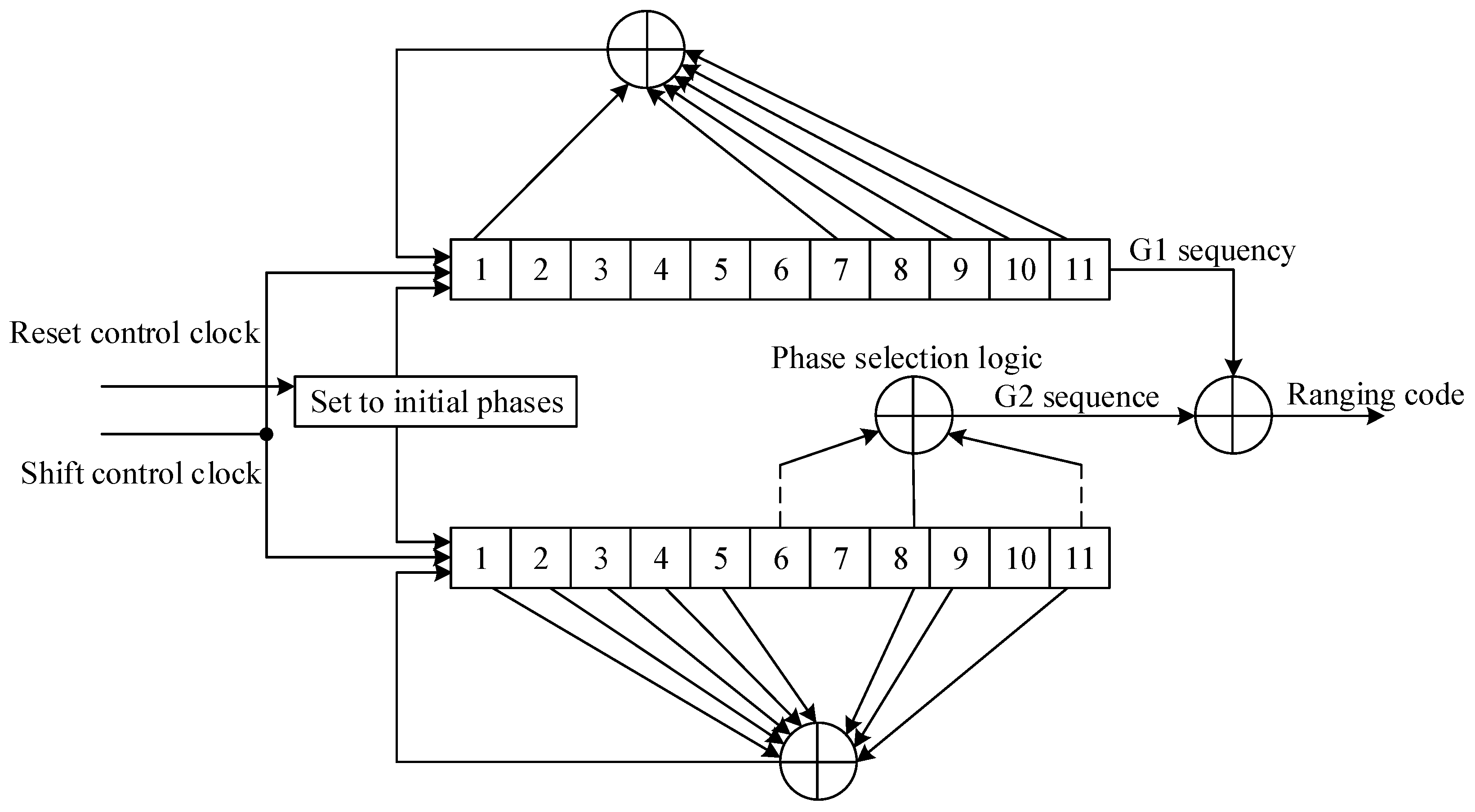
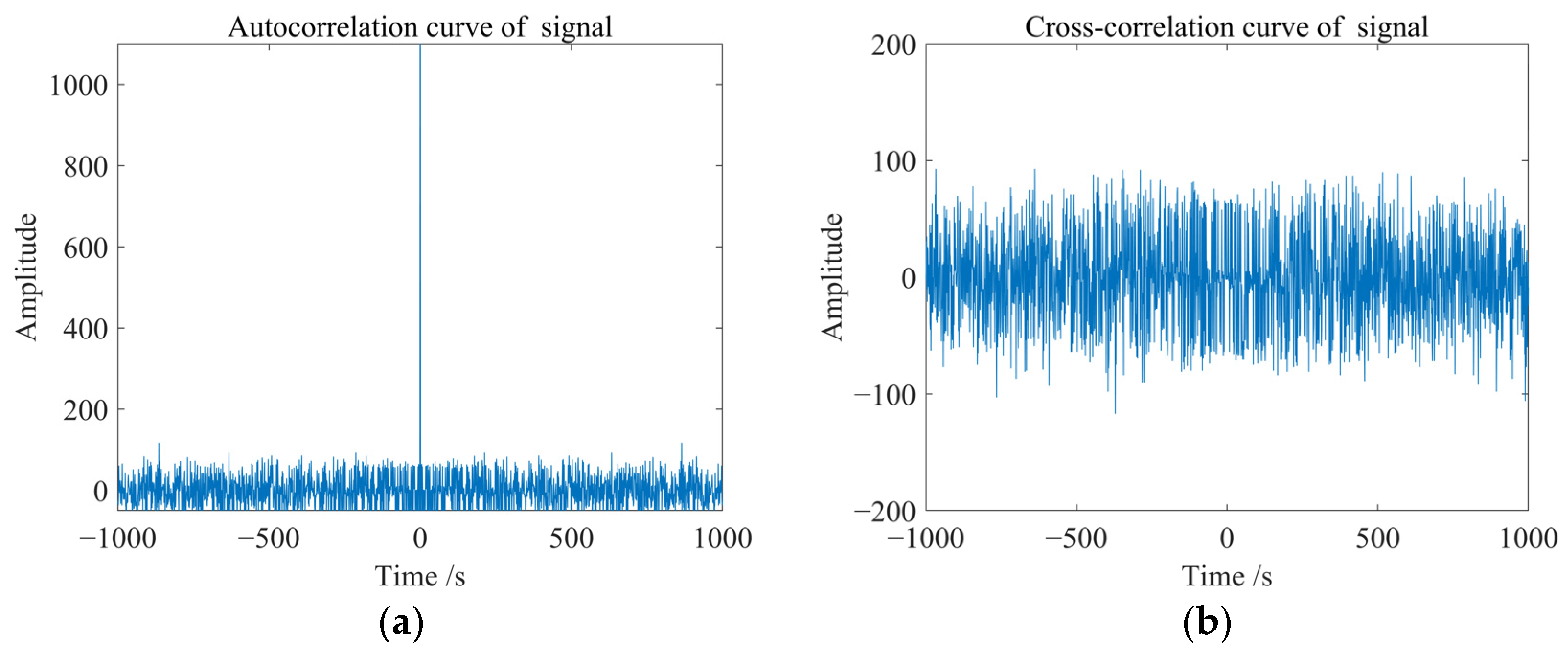
The specific generation method of the CA code is shown in Figure 1 according to reference [34]. The B1I signal ranging code (${\mathrm{C}}_{\mathrm{B}1\mathrm{I}}$) is a periodic sequence composed of 2046 chips with a period of 1 ms. It is generated by the module-2 operation of two linear sequences G1 and G2 to produce balanced Gold codes and then truncating the last chip. The unique PRN of each satellite determines the generation of its G2 sequence, so each satellite has a unique ranging code. In this study, satellites 19 and 20 are selected as examples, with the generation method of their G2 sequences presented in

Table 1. Phase assignment of G2 sequence.

Satellite ID	Satellite Type	Ranging Code Number	Phase Assignment of G2 Sequence
19	MEO/IGSO satellite	19	$4\oplus 8$
20	MEO/IGSO satellite	20	$4\oplus 9$

. Subsequently, the B1I signals of the two satellites are generated according to Equation (1), and their autocorrelation and cross-correlation characteristics are analyzed. The correlation curve of the B1I code BDS signal is shown in Figure 2. The image clearly shows that different pseudo-random codes ensure the orthogonality between different satellite signals.

The satellite’s navigation message (${\mathrm{D}}_{\mathrm{B}1\mathrm{I}}$) contains the basic navigation data of the satellite, all the satellite almanac data, as well as the time synchronization information with other systems, which can be used to calculate the satellite’s position, speed, and other information. Among them, the D1 navigation message is modulated by the Neumann-Hoffman code (also known as NH code). As shown in Figure 3, a navigation message in the D1 navigation message is 20 ms, and the spread spectrum code period is 1 ms. Therefore, the 20-bit length NH code [0 0 0 0 0 0 1 0 0 0 1 1 0 1 0 1 0 1 0 0 1 1 1 0] with a code rate of 1 kbps and a code width of 1 ms is used, which is modulated with the spread-spectrum code and the navigation information code using the module-2 addition.

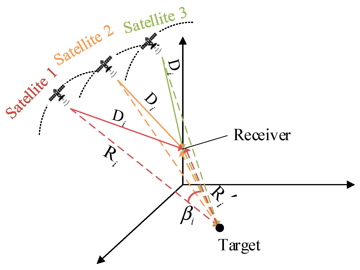
In comprehensively utilizing the navigation satellite signals of various globally available GNSSs, the transmit–receive multistatic detection scheme based on the MIMO signal processing method can be adopted. The receiving station can be arranged on the ground, ships, aircraft, and even low-orbit satellite platforms. This paper focuses on the multi-transmit, single-receiver radar system, and its system structure is shown in Figure 4.

The distance from the GNSS satellite i to the receiver is ${\mathrm{D}}_i$, the propagation distance from the signal scattered by the ground moving target to the receiver is ${\mathrm{R}}_i+{{\mathrm{R}}_i}^{\prime }$, and the double base angle formed by the satellite, the target, and the receiver is ${\beta }_i$. The direct signal propagation delay and the scattered signal propagation delay are ${\tau }_{\mathrm{d}}$ and ${\tau }_{\mathrm{s}}$, respectively, where $\mathrm{c}$ represents the speed of light:

$${\tau }_{\mathrm{d}}={\displaystyle \frac{{\mathrm{D}}_i}{\mathrm{c}}}$$

(2)

$${\tau }_{\mathrm{s}}={\displaystyle \frac{{\mathrm{R}}_i+{{\mathrm{R}}_i}^{\prime }}{\mathrm{c}}}$$

(3)

The Doppler frequency of the received signal is $f_{\mathrm{d}}$ when the target is moving at a speed of $v$:

$$f_{\mathrm{d}}={\displaystyle \frac{2v}{\lambda }}\cos \delta \cos {\displaystyle \frac{\beta }{2}}$$

(4)

where $\delta$ is the angle between the velocity vector and the bistatic angle bisector, $\beta$ is the double base angle, and $\lambda$ represents the signal wavelength.

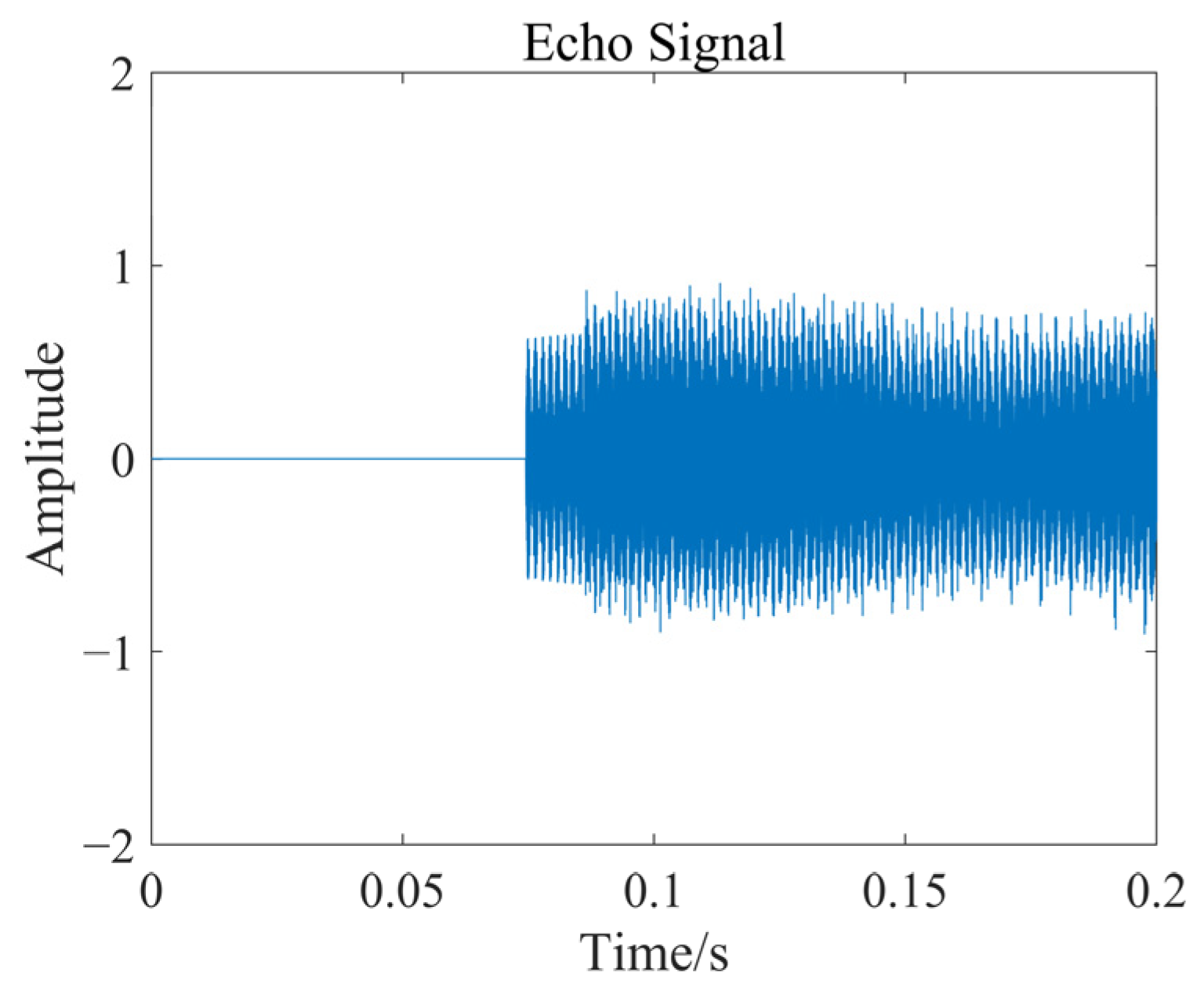
According to Equation (1), the bistatic scene detection echo can be further expanded as the following:

$$\begin{array}{ll}{\mathrm{S}}_{\mathrm{s}}& ={\mathrm{S}}_{\mathrm{d}}+{\mathrm{S}}_{\mathrm{s}}\\ & ={\displaystyle \sum _{i=1}^{\mathrm{M}}{a}_{\mathrm{d}}^{\left(i\right)}\mathrm{A}{\mathrm{C}}^{\left(i\right)}\left(t\right){\mathrm{D}}^{\left(i\right)}\left(t\right)\cos \left(2\pi \left(f_0+f_{\mathrm{d}\text{-}\mathrm{d}}^{\left(i\right)}\right)\left(t-{\tau }_{\mathrm{d}}^{\left(i\right)}\right)+{\phi }_{\mathrm{d}}^{\left(i\right)}\right)}+\\ & {\displaystyle \sum _{i=1}^{\mathrm{M}}{\displaystyle \sum _{j=1}^{\mathrm{Q}}{a}_{\mathrm{s}}^{\left(i\right),\left(j\right)}\mathrm{A}{\mathrm{C}}^{\left(i\right)}\left(t\right){\mathrm{D}}^{\left(i\right)}\left(t\right)\cos \left(2\pi \left(f_0+f_{\mathrm{d}\text{-}\mathrm{s}}^{\left(i\right),\left(j\right)}\right)\left(t-{\tau }_{\mathrm{s}}^{\left(i\right),\left(j\right)}\right)+{\phi }_{\mathrm{s}}^{\left(i\right),\left(j\right)}\right)}}\end{array}$$

(5)

where ${\mathrm{S}}_{\mathrm{d}}$ represents the direct echo signal, ${\mathrm{S}}_{\mathrm{s}}$ represents the scattered echo signal, and $a$ is the propagation coefficient. According to Equation (5), the signal echo is transmitted by $\mathrm{M}$ satellite, reflected by $\mathrm{Q}$ target, and then linearly superimposed in the time domain at the receiver.

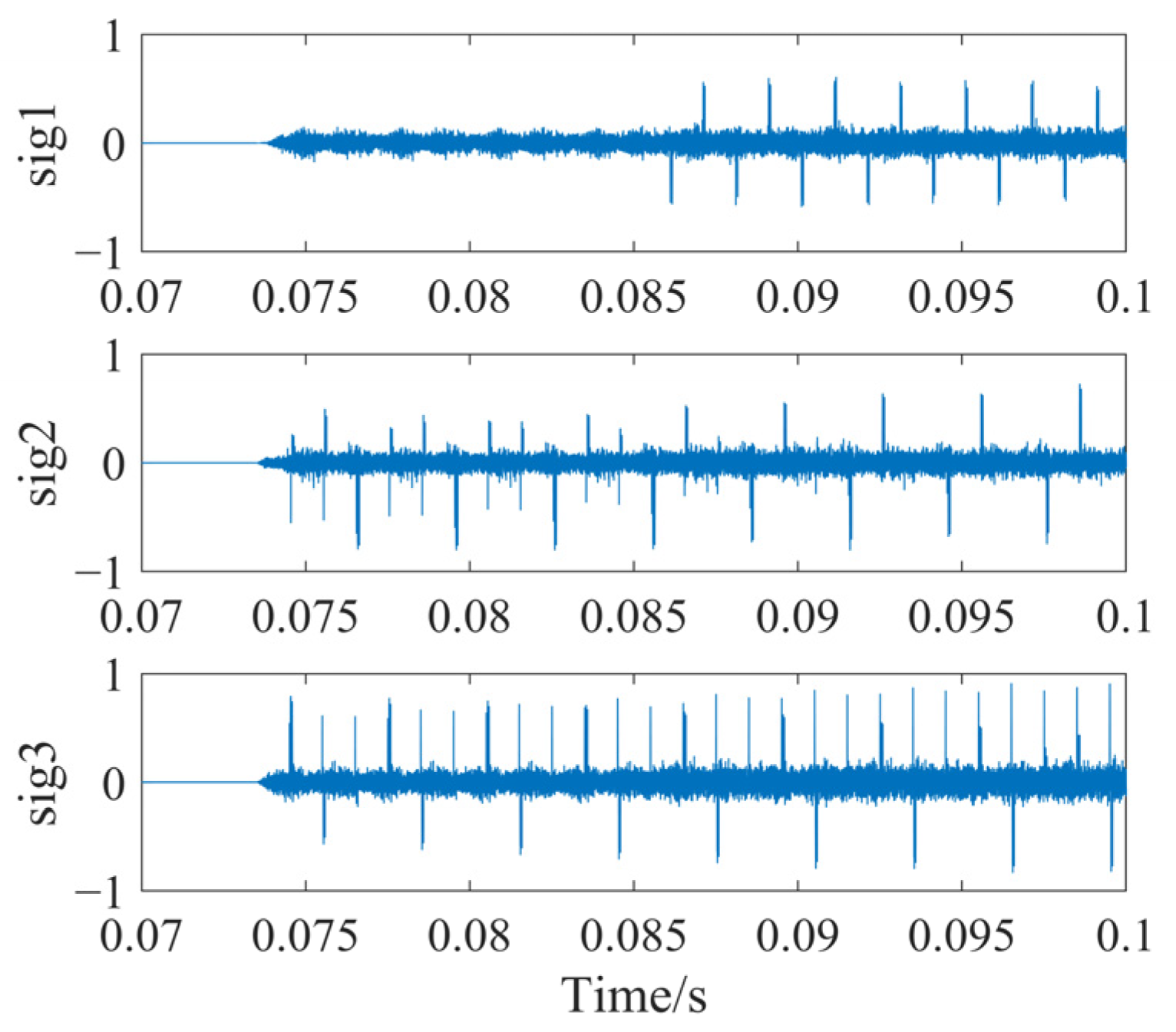
A single satellite can simultaneously transmit information on multiple frequency bands. Utilizing signals from multiple frequency bands helps GNSS receivers more accurately determine the propagation path of the satellite signals and enhances resistance to multipath effects, thereby achieving more reliable and precise positioning services. This paper selects the B1I and B3I signals, which are simultaneously transmitted by satellites in the BDS, with carrier frequencies of 1561.098 MHz and 1268.52 MHz, respectively. According to Equation (4), the Doppler frequency shift in the signal is related to the target velocity, signal wavelength, and geometric configuration. Since the signals are transmitted by the same satellite and received by the same receiver, with identical velocity and bistatic configuration, only the differences in signal wavelength need to be considered. Therefore, it is necessary to define the phase ratio factor for signals of different frequency bands in Equation (6) [36].

$$k={\displaystyle \frac{f_{c1}}{f_{c2}}}={\displaystyle \frac{{\lambda }_2}{{\lambda }_1}}$$

(6)

Substituting Equation (4) into Equation (5) and completing the carrier removal at the receiver, the detected echo with carrier frequency $f_{c2}$ multiplied by the scale factor $k$ takes the following form for the multi-satellite detection signal, achieving the phase alignment of different signals from the same satellite:

$$\begin{array}{ll}{\mathrm{S}}_{\mathrm{t}\mathrm{o}\mathrm{t}\mathrm{a}\mathrm{l}}& ={\mathrm{S}}_{\mathrm{s}1}+{\mathrm{S}}_{\mathrm{s}2}\\ & ={\displaystyle \sum _{i=1}^{\mathrm{M}}{a}^{\left(i\right)}\mathrm{A}{\mathrm{C}}^{\left(i\right)}\left(t\right){\mathrm{D}}^{\left(i\right)}\left(t\right)\cos \left(2\pi \left(\frac{2v}{{\lambda }_1}\cos \delta \cos \frac{\beta }{2}\right)\left(t-{\tau }^{\left(i\right)}\right)+{\phi }^{\left(i\right)}\right)}+\\ & {\displaystyle \sum _{i=1}^{\mathrm{M}}{b}^{\left(i\right)}\mathrm{A}{\mathrm{C}}^{\left(i\right)}\left(t\right){\mathrm{D}}^{\left(i\right)}\left(t\right)\cos \left(2\pi \left(k\cdot \frac{2v}{{\lambda }_2}\cos \delta \cos \frac{\beta }{2}\right)\left(t-{\tau }^{\left(i\right)}\right)+{\phi }^{\left(i\right)}\right)}\end{array}$$

(7)

The navigation code information is obtained by matching filtering the echo with the product of the local ranging code and the acquisition code. The navigation code consists of 8 bits, with each bit lasting 20 milliseconds., and the given navigation code in the simulation is $\mathrm{c}\mathrm{o}\mathrm{d}\mathrm{e}\_\mathrm{n}\mathrm{a}\mathrm{v}=\left[1 0 1 0 0 1 1 0\right]$.

After acquiring the navigation code, the navigation code is demodulated and multiplied with the echo signal about the first peak position.

$$s_{\mathrm{r}}=s_{\mathrm{r}}\cdot {\displaystyle \sum _{j=1}^{\mathrm{J}}{u}_{160\cdot T_p}\left(t-t_0^{\left(j\right)}\right)D^{\left(j\right)\prime }}$$

(8)

where $u_{160\cdot T_p}\left(t-t_0^{\left(j\right)}\right)$ is the window function, the pulse repetition time $T_p$ is 1 ms, and $160\cdot T_p$ represents the length of the window function, which is 160 times $T_p$. $t_0^{\left(j\right)}$ is the first target peak moment, and $D^{\left(j\right)\prime }$ is the navigation code filtered by the j-th satellite signal. The offset due to the delay of the target echo affects the correlation amplitude of only 1 out of 20 ranging codes per navigation code, and this offset has a negligible effect on the target correlation detection amplitude after accumulating multiple ranging code cycles on the results.

3. Simulation of Multi-Satellite, Multi-Target Detection Model

3.1. RDM Simulation and Information Inversion of Ideal Point Targets

In this section, three oblique orbiting satellites with PRN codes 4, 26, and 31 in BDS are simulated to transmit signals for the detection of three point targets. The target parameters are given in

Table 2. Parameters of the targets.

Parameters	Target 1	Target 2	Target 3
Location/m	(−9526, 5500, −60)	(−1414, 1414, −60)	(750, 1299, −60)
Velocity/m × s−1	120	80	80
RCS/m2	1	1	1

. The sampling frequency of the B1I signal is 8.184 MHz, while that of the B3I signal is 40.92 MHz. The coherent integration time is 128 ms. The echo signal received by the receiver at a fixed position is shown in Figure 5. It can be seen that the signal is transmitted at the moment 0 s and the echo signal is first received at 0.075 s. The direct signal arrives at the receiver first and is linearly superimposed with the scattered echoes that arrive at the receiver later. It is also due to the RCS, transmission loss, and other factors of the target that lead to different amplitudes of the echo signal. After superposition, the time-domain image of the echo signal exhibits envelope fluctuations.

In addition, the echo signal is further processed to demodulate the ranging codes of different satellites. Since direct signals propagate without undergoing scattering weakening and travel over shorter distances, they usually have a higher amplitude in the echo, which may sometimes overwhelm the target signal. After demodulation, the peak of the direct signal in the echo is more significant, and the time-domain location of the first direct signal peak of each of the three satellite signals is given in Figure 6. The first peak of the signal reflects the direct signal delay information, which can be used to complete the pre-processing of the target distance and provide rationality for the local imaging range setting later.

Table 3. Direct distance data table.

Sat. ID	First Peak Moment/s	Estimated Distance/m	Actual Distance/m	Estimated Error/m	Relative Error
4	0.08609	25,826,150.98	25,826,138.21	12.78	0.00005%
26	0.07455	22,364,853.79	22,365,108.60	108.18	0.00048%
31	0.07451	22,352,097.16	22,352,312.84	69.05	0.00031%

lists the calculated direct distances based on the image information, as well as the true distance data. There is a certain gap between the two distances, but the error is small.

Next, the B1I and B3I signals of the three satellites were simulated, which have bandwidths of 4.092 MHz and 20.46 MHz, respectively. The starting distances were selected as 25,826 km, 22,365 km, and 22,352 km to ensure that both direct and target points were included in the partial imaging. Assuming that each satellite transmits the above two signals at the same time, six signals transmitted by three satellites can be received at the receiver and then processed.

The target RDMs illuminated by the B1I and B3I signals are plotted in Figure 7. We can find that the peak of the direct signal is separated from the peak of the target point echo in both distance and Doppler dimensions. According to the theory of the model, the peak located at the closest distance in the image is the direct signal in the echo. At the same time, due to the different direction of target movement, double base angle, and distance, the distribution of the point targets in different dimensions and scattering intensities under the irradiation of the three satellites also produce large differences, which can also illustrate that the spatially distributed MIMO radar is able to detect more comprehensive information about the features from multiple perspectives.

By using multi-satellite simulations to detect the same set of multiple targets, we can combine the results from different satellites to more accurately invert and analyze the distance information of each target. After using ranging codes to distinguish the detection results from different satellites, the various time delay information and Doppler frequencies from multi-satellite target detection are combined with satellite and receiver data, which are then jointly solved to obtain the inversion results for the precise location and velocity of the targets. The formulas for inversion are as follows:

$$r^{i,j}=\sqrt{{\left(x_s^i-x_t^j\right)}^2+{\left(y_s^i-y_t^j\right)}^2+{\left(z_s^i-z_t^j\right)}^2}+\sqrt{{\left(x_r-x_t^j\right)}^2+{\left(y_r-y_t^j\right)}^2+{\left(z_r-z_t^j\right)}^2}$$

(9)

$$f_d^j={\displaystyle \frac{2v_j}{{\lambda }_i}}\cos {\delta }_j\cos {\displaystyle \frac{{\beta }_j}{2}}$$

(10)

where $i$ represents the satellite ID, $j$ represents the target ID, $r^{i,j}$ is the signal scattering distance, and $\left(x,y,z\right)$ denotes the three-dimensional coordinates. The subscripts $s$, $t$, and $r$ refer to the satellite, target, and receiver, respectively.

Table 4. Position inversion information.

Target ID	Actual $\left(\mathit{x},\mathit{y},\mathit{z}\right)$/m	Estimated $\left(\mathit{x},\mathit{y},\mathit{z}\right)$/m	$\left(\Delta \mathit{x},\Delta \mathit{y},\Delta \mathit{z}\right)$/m
1	(−9526.28, 5500, −60)	(−9537.32, 5484.60, −48.55)	(11.04, 15.40, 11.45)
2	(−1414.21, 1414.21, −60)	(−1413.60, 1410.86, −57.18)	(0.62, 3.36, 2.82)
3	(750, 1299.04, −60)	(790.28, 1311.34, −72.12)	(40.28, 12.30, 12.12)

shows the position inversion data for the three point targets. For this simulation, the distance errors obtained with satellites 4, 26, and 31 range from 4 to 43 m. The calculated velocities produced errors of 0.84%, 1.11%, and 1.11%, respectively. Therefore, it can be preliminarily concluded that the results obtained through multi-satellite joint solving are reliable.

At the same time, due to the variation in geometrical configurations in the scattering model and the influence of the speed of the moving target, there are differences in the distance resolution of target detection by different satellites.

Table 5. The range resolution of B1I signal.

Distance Resolution/m	Target 1	Target 2	Target 3
Satellite 4	79.19	91.58	102.88
Satellite 26	73.71	77.50	83.05
Satellite 31	75.60	79.05	85.39

and

Table 6. The range resolution of B3I signal.

Distance Resolution/m	Target 1	Target 2	Target 3
Satellite 4	15.24	18.32	20.58
Satellite 26	14.74	15.50	16.61
Satellite 31	15.12	15.81	17.07

provide the differences in distance resolution produced by the B1I and B3I signals in the same geometric configuration. The Doppler phase effect of the target’s speed brings more challenges for target detection in all kinds of complex scenes.

3.2. RDM Simulation and Information Inversion of Real Targets

In the RDM simulation of point targets, our approach begins with echo simulation, continues with echo processing to achieve RDM imaging, and concludes with target information inversion. However, when simulating the RDM of large targets, an electromagnetic scattering model is needed to calculate the target’s scattering characteristics, ensuring accurate echo simulation. To balance computational accuracy and efficiency, we have chosen the GO-PO (Geometric Optics and Physical Optics) method for these calculations. The GO-PO method is a high-frequency approximation technique that effectively calculates multiple scattering from targets [28]. First, the target model is divided into several triangular patches. When an electromagnetic wave strikes one of these patches, the far-field scattering of a single patch can be expressed using the Stratton–Chu integral equation as follows:

$$E_{pq}(\mathit{r})={\displaystyle \frac{\exp (\mathrm{j}kR)}{4\pi R}}\left[\widehat{\mathit{q}}\cdot {\widehat{\mathit{k}}}_{\mathrm{s}}\times \right.\left({\mathit{M}}_0\right.\left.\left.-\eta {\widehat{\mathit{k}}}_{\mathrm{s}}\times {\mathit{J}}_0\right)\right]\cdot I$$

(11)

where $\mathit{r}$ is the center position of the patch, $\exp (\mathrm{j}kR)/4\pi R$ is the Green’s function for the far field, $k$ is the wavenumber of the electromagnetic wave, and $R$ is the distance between the center of the patch and the observation point. $\widehat{\mathit{q}}$ represents the unit polarization vector of the scattered wave, and ${\widehat{\mathit{k}}}_{\mathrm{s}}$ represents the wave vector of the scattered wave; $\eta$ is the intrinsic impedance. ${\mathit{M}}_0$ and ${\mathit{J}}_0$ represent the induced magnetic and electric currents, respectively. And $I$ represents the phase integral. According to the Gordon method, its specific calculation expression is as follows:

$$\begin{array}{ll}I& =\mathrm{j}k{\displaystyle \int \exp \left[\mathrm{j}k\left({\widehat{\mathit{k}}}_{\mathrm{i}}-{\widehat{\mathit{k}}}_{\mathrm{s}}\right)\cdot {\mathit{r}}^{\prime }\right]}\mathrm{d}{\mathrm{s}}^{\prime }\\ & ={\displaystyle \frac{\exp \left(\mathrm{j}k{\mathit{r}}_0\cdot \mathit{w}\right)}{T}}{\displaystyle \sum _{m=1}^M\left(\widehat{\mathit{p}}\cdot {\mathit{a}}_m\right)}\exp \left(\mathrm{j}k{\mathit{b}}_m\cdot \mathit{w}\right){\displaystyle \frac{\sin \left(k{\mathit{a}}_{\mathit{m}}\cdot \mathit{w}/2\right)}{k{\mathit{a}}_{\mathit{m}}\cdot \mathit{w}/2}}\end{array}$$

(12)

where ${\widehat{\mathit{k}}}_{\mathrm{i}}$ is the incident wave vector, ${\mathit{r}}^{\prime }$ is the position vector from the local origin to the surface patch $\mathrm{d}{s}^{\prime }$, $M$ denotes the number of sides of the patch, and ${\mathit{r}}_0$ represents the centroid vector of the patch. Then, $\widehat{\mathit{n}}$ is the unit normal vector of the patch, $\mathit{w}={\widehat{\mathit{k}}}_{\mathrm{i}}-{\widehat{\mathit{k}}}_{\mathrm{s}}$, $\widehat{\mathit{p}}=\widehat{\mathit{n}}\times \mathit{w}/\left|\widehat{\mathit{n}}\times \mathit{w}\right|$, ${\mathit{a}}_m={\mathit{r}}_{m+1}-{\mathit{r}}_m$, ${\mathit{b}}_m=\left({\mathit{r}}_{m+1}+{\mathit{r}}_m\right)/2$, and $T$ is the length of the projection of $\mathit{w}$ on the patch.

Thus, the total single scattering field can be expressed as follows:

$${\mathit{E}}_{pq}^1={\displaystyle \sum _{m=1}^N{E}_{pq,m}}\left(r_m\right)\cdot I_{vi\mathrm{s},m}$$

(13)

where $N$ represents the total number of patches on the target, and $I_{vi\mathrm{s},m}$ represents the visibility factor of patch $m$ with respect to the incident wave. If patch $m$ is illuminated by the incident wave, then $I_{vi\mathrm{s},m}=1$; otherwise, $I_{vi\mathrm{s},m}=0$.

If patch $n$ is illuminated by the reflected wave from patch $m$, then the secondary scattering field can be expressed as follows:

$${\mathit{E}}_{pq}^2={\displaystyle \frac{\exp (\mathrm{j}kR)}{4\pi R}}{\displaystyle \sum _{n=1}^N\left[\widehat{\mathit{q}}\cdot {\widehat{\mathit{k}}}_{\mathrm{s}}\times \left({\displaystyle \sum _{m=1}^N{I}_{vis,m}\cdot }{\mathit{M}}_{1,nm}\cdot I_{vis,nm}-\eta {\widehat{\mathit{k}}}_{\mathrm{s}}\times {\displaystyle \sum _{m=1}^M{I}_{vis,m}\cdot }{\mathit{J}}_{1,nm}\cdot I_{vis,nm}\right)\right]}\cdot I_n$$

(14)

where ${\mathit{M}}_{1,nm}$ is the induced magnetic current and ${\mathit{J}}_{1,nm}$ is the induced electric current of the first reflection field on patch $n$. $I_{vis,nm}$ is the visibility factor.

Finally, the total scattering field of the three-dimensional target can be expressed as the sum of the single scattering field and the multiple scattering fields, as follows:

$${\mathit{E}}_{pq}^{target}\left({\widehat{\mathit{k}}}_i,{\widehat{\mathit{k}}}_{\mathrm{s}}\right)={\displaystyle \sum _{n=1}^N\frac{\exp (\mathrm{j}kR)}{4\pi R}\left[\widehat{\mathit{q}}\cdot {\widehat{\mathit{k}}}_{\mathrm{s}}\times \left({\mathit{M}}_n-\eta {\widehat{\mathit{k}}}_{\mathrm{s}}\times {\mathit{J}}_n\right)\right]\cdot I_n}$$

(15)

This allows for the calculation of the scattering characteristics of sea surface ship targets, facilitating subsequent imaging simulations.

When large ship targets navigate at sea, their translational motion causes Doppler frequency effects. If the radial velocity of the ship is significant, the sign of the Doppler center frequency of the range cell containing the ship will match the sign of the Doppler frequency caused by the translation. Furthermore, because the ship is a rigid body target, all scattering points adhere to the rigid body motion, resulting in minimal differences in the Doppler center frequencies between individual scattering points. In scenarios where the ship target exhibits a strong scattering intensity, the Doppler spectrum of the target is concentrated, allowing effective extraction of the distance unit information containing the ship target from the range profile. Due to the impact of bistatic angles in the detection model on imaging distance resolution, it is necessary to simulate geometrical configurations with smaller bistatic angles to achieve higher distance resolution. The real-time positions of the satellites are derived from the ephemeris data, sourced from the IGS Center, Wuhan University [37]. Data from the 264th day of 2023, i.e., 21 September 2023, is selected. Based on the real-time positions of satellites, satellites numbered 8, 14, and 27 were selected to complete the simulation of ship target detection, as shown in Figure 8.

The range-Doppler algorithm transforms the energy of strong scattering points with the same range but different azimuths into the azimuth frequency domain, causing their positions to overlap in the image. The area between the red lines in the image represents the distribution range of the scattering points on the first ship’s body. The region between the green lines illustrates the distribution of the second ship, which is positioned 1 km from the first ship.

The following provides a detailed analysis of ship #1. By calculating the distance between the clusters of strong scattering points, an estimate of the ship’s length can be obtained. In the image obtained from the B1I band, the distribution of strong scattering points spans two resolution cells, which inevitably causes an elongation in the estimated ship’s length. The estimated length is approximately 293 m, with an error of up to 130%. In the B3I band, this issue is improved. The strong scattering point clusters are distributed between 88 and 146 m, and the estimated ship’s length error ranges from 7% to 11%, showing a significant improvement compared to the results from the B1I band. It can be observed that the Doppler information reflected by the two signals closely matches, accurately indicating the direction of the target’s velocity. The ship’s length detected by the B3I signal aligns with the actual ship’s length, whereas the results obtained from the B1I signal, which has poorer distance resolution, elongate the ship target in the range direction, causing distortion in the ship’s length information. Based on Equations (9) and (10), the strong scattering point clusters of the target ship are situated within a region in the coordinate system centered at (−18.785, 39.913, 8.107). The computed ship #1 velocity is 97.05 m/s in the positive y-direction, with a 3% deviation from the expected value. Additionally, ship #2 is located at (857.826, 1123.528, −37.161) with a velocity of 21.42 m/s and a velocity error of 7.1%, as shown in

Table 7. Inversion results of ship characteristic values.

ID	Estimated Center Position/m	Estimated Velocity/m · s−1	Velocity Error
1	(−18.785, 39.913, 8.107)	97.05	3%
2	(857.826, 1123.528, −37.161)	21.42	7.1%

.

4. Multi-Satellite Information Fusion and Positioning Optimization

To achieve the continuous and accurate estimation of target motion parameters, it is essential to address the fusion of multi-source heterogeneous observation data at the state estimation level. However, in GNSS-based target detection systems, the inversion and tracking of target information are significantly affected by the nonlinear motion of the target and non-Gaussian noise in complex environments. Therefore, selecting an appropriate filtering algorithm largely determines the accuracy of the navigation system. This paper proposes the use of the UPF algorithm for dynamic tracking of moving targets and analyzes the differences in the results between three-satellite and four-satellite solutions.

4.1. Unscented Particle Filter Information Fusion Algorithm

Step 1: Particle Initialization: A set of randomly distributed particles, ${\left\{x_0^i\right\}}_{i=1}^N$, is drawn from the initial state distribution $p\left(x_0\right)$ to simulate the uncertainty of the system state. All particles are assigned equal weights:

$$w_0^i={\displaystyle \frac{1}{N}}, i=1,2,\cdots N$$

(16)

where $N$ is the number of particles.

Step 2: State Estimation Using UKF: For each particle $x_{k-1}^i$, use UKF to generate sigma points, and then compute the predicted state mean and covariance matrix.

Step 3: Importance Sampling Distribution: Using the sigma point generation formula, calculate the proposal distribution for the particles. Perform particle sampling within this distribution to enhance the efficiency of particle sampling.

Step 4: Particle Weighting: The weight of each particle is updated based on the current observation $z_k$ and the particle position $x_k^i$, using the likelihood function $p\left(\left.z_k\right|x_k^i\right)$ of the observation. The weights are then normalized.

$$w_k^i=w_{k-1}^i\cdot p\left(\left.z_k\right|x_k^i\right)$$

(17)

$$w_k^i={\displaystyle \frac{w_k^i}{{\displaystyle \sum _{j=1}^N{w}_k^j}}}$$

(18)

The particle weight directly reflects the degree of match between the corresponding sample and the true posterior distribution of the target. A higher weight indicates that the particle is more likely to generate the observed data, meaning its state estimate is closer to the true system state, thus carrying a higher confidence within the probability distribution space.

Step 5: Particle Resampling: The purpose of resampling is to generate a new set of particles from the current particle set, selecting particles with high weights and eliminating those with low weights. After resampling, the weights of the particles are set to be equal.

Step 6: State Estimation: After resampling, the state estimate is obtained as the weighted average of the particle set.

$${\widehat{x}}_k={\displaystyle \sum _{i=1}^N{w}_k^i{x}_k^i}$$

(19)

Step 7: Repeat the above steps until all observation data have been processed.

As can be seen, the UPF uses the UKF to generate the importance sampling distribution, leveraging the deterministic sampling of the unscented transformation and the Monte Carlo nature of particle filtering. This allows particles to be more effectively distributed in the state space. Compared to the simple random sampling in traditional particle filters, this significantly improves the representativeness and sampling efficiency of the particles. Therefore, UPF notably enhances the EKF’s ability to handle complex nonlinear systems and improve estimation accuracy.

4.2. Analysis of UPF Results

In the simulation, a three-satellite observation scenario is constructed using satellites with PRNs 4, 26, and 31. A four-satellite scenario is formed by additionally incorporating the satellite with PRN 21. The positional parameters of these satellites are listed in

Table 8. Satellite position parameters.

ID	X Coordinate/m	Y Coordinate/m	Z Coordinate/m
4	21,012,136.4	−15,015,077.6	−157,769.8
26	16,846,204.6	−5,502,126.7	13,649,449.7
31	18,022,429.8	1,093,667.2	13,183,062.8
21	−21,912,642.7	−14,678,690.7	−1,502,695.6

.

(1)

Computation results of position and velocity for uniformly moving targets.

The following analysis is based on a 40 s dynamic scenario simulation with a sampling interval of 128 ms. To evaluate the tracking performance of the algorithm for uniformly moving targets, a dynamic positioning scenario is designed as follows:

The target is initialized at position (−9526, 5500, −60) and moves at a constant velocity of 120 m/s along the y-axis. The receiver is fixed at position (0, 0, 6500).

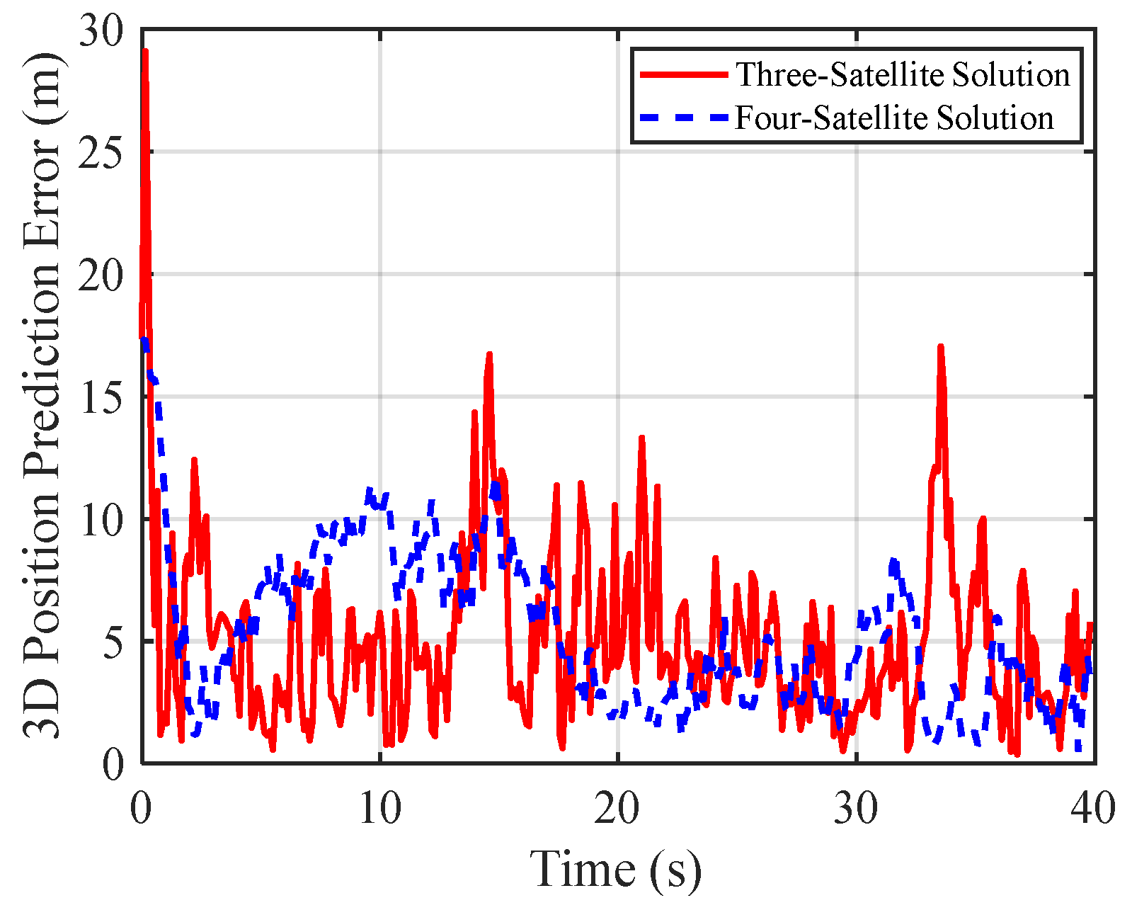
Figure 9 and Figure 10 compare the 3D position errors obtained from three-satellite and four-satellite solutions. It is evident that the number of satellites has a significant impact on both positioning accuracy and stability. Experimental results show that when using four satellites, the mean position error remains strictly within 10 m, and the variance of the error is confined to within 5 m², indicating high accuracy and stability. In contrast, the three-satellite solution yields a wider error distribution, with position errors reaching up to 18 m and error variances ranging from 10 to 50 m², along with more pronounced fluctuations. This phenomenon suggests that increasing the number of visible satellites from three to four enhances the redundancy of the observation equations, facilitating a more optimal estimation of the predicted position, and thereby reducing the sensitivity of the solution to individual satellite measurement errors.

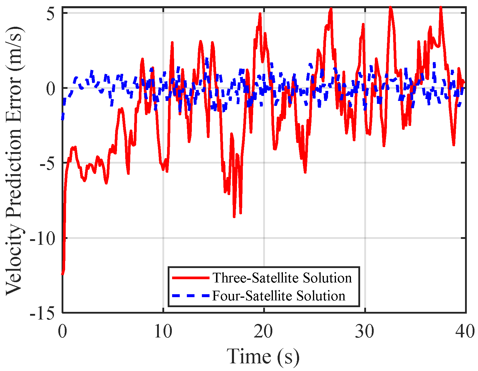
Figure 11 and Figure 12 compare the velocity errors obtained from three-satellite and four-satellite solutions. Experimental data indicate that under the four-satellite scenario, the predicted velocity error remains strictly within ±2 m/s, with a variance upper bound of 3 (m/s)². In contrast, the three-satellite solution exhibits a broader error range of up to ±7 m/s, with error variances ranging from 10 to 40 (m/s)², indicating a higher degree of uncertainty in velocity prediction. This observation demonstrates that the incorporation of additional satellite observations enables more accurate and stable velocity estimation with reduced fluctuations.

(2)

Computation results of position and velocity for non-uniformly moving targets.

To validate the algorithm’s performance, this simulation designs a dynamic positioning scenario consistent with Simulation 2 in the three-satellite analysis. The target’s initial position is set at (−9526, 5500, −60), moving along the y-axis with uniform acceleration, starting at an initial velocity of 60 m/s and an acceleration of 1 m/s². The receiver is fixed at position (0, 0, 6500), while the satellite positions correspond to those listed in Table 8.

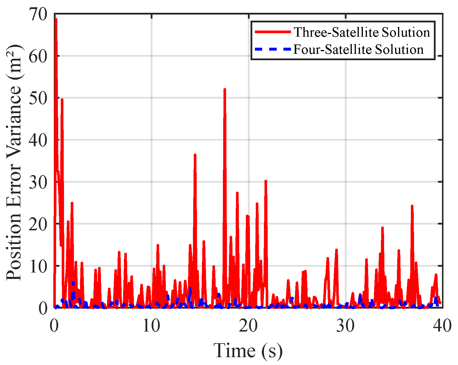
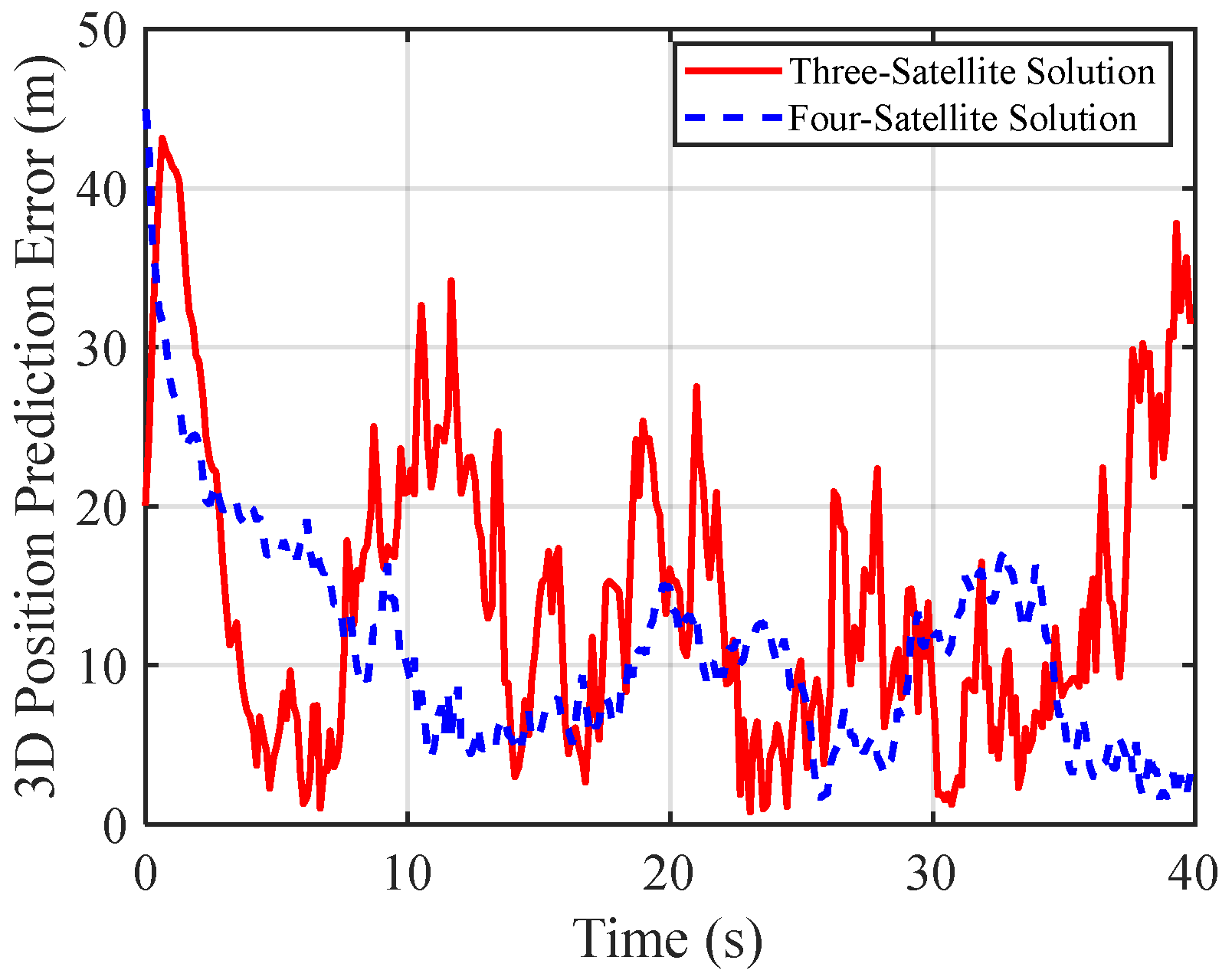
Figure 13 and Figure 14 compare the 3D position errors from three-satellite and four-satellite solutions under accelerated motion. The results show that the mean position error for the four-satellite solution remains within 18 m, representing a reduction of approximately 40% to 60% compared to the three-satellite system. The position error variance is strictly controlled within 5 m², whereas the variance range for the three-satellite solution expands significantly to between 20 and 75 m², exhibiting a pronounced heteroscedasticity that indicates greater instability in the three-satellite solution. These findings further demonstrate that the four-satellite solution outperforms the three-satellite solution in both accuracy and stability for the 3D positioning of targets undergoing accelerated motion.

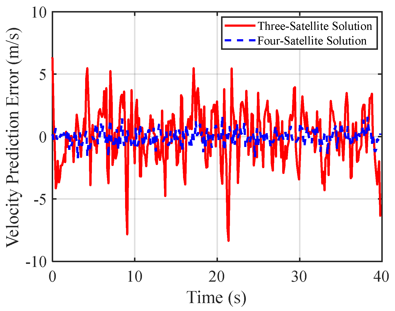
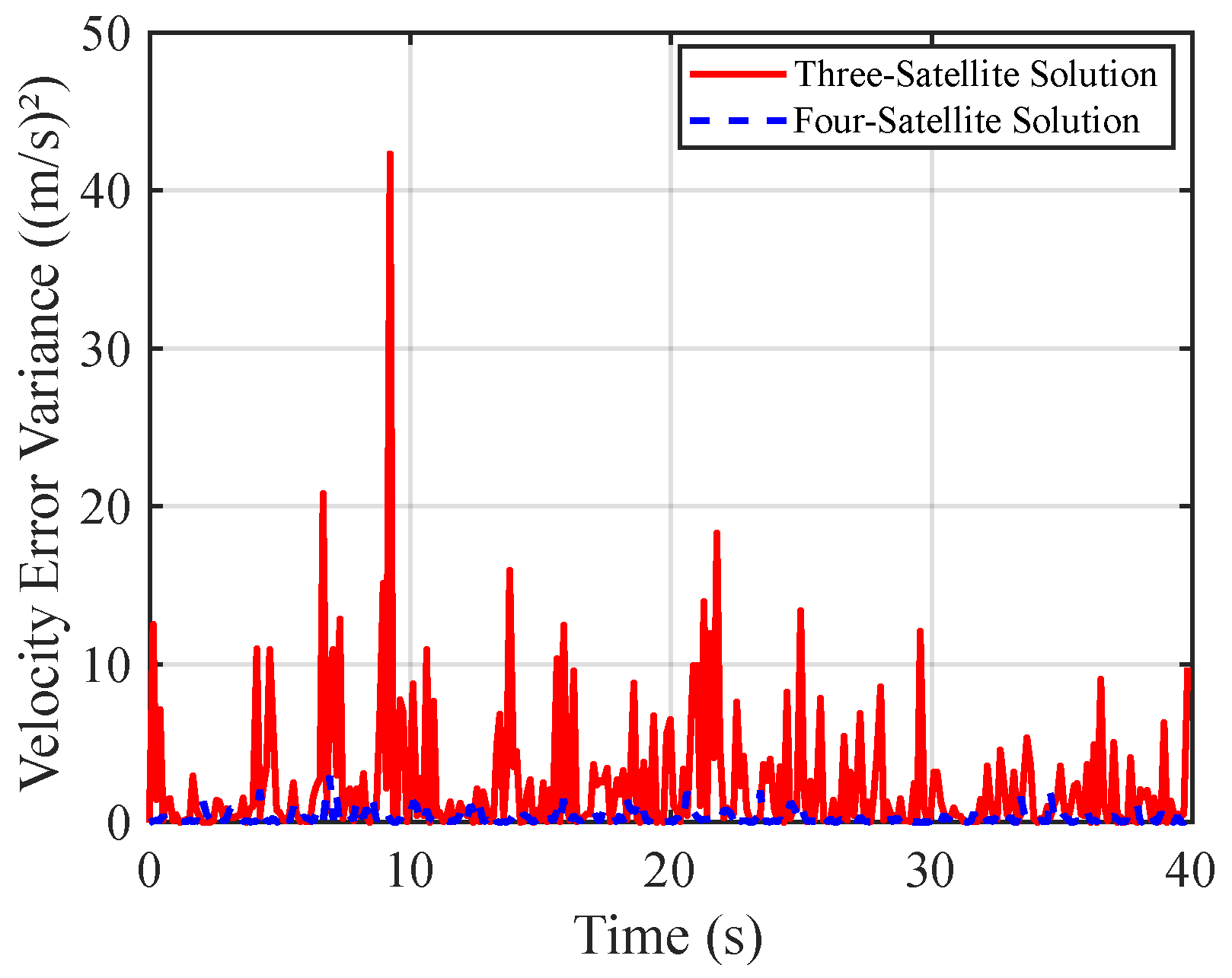
Figure 15 and Figure 16 compare the velocity errors obtained from three-satellite and four-satellite solutions. Experimental data in Figure 15 show that the velocity error in the four-satellite solution is strictly controlled within ±2 m/s, with the fluctuation amplitude only 25% of that observed in the three-satellite solution, which reaches ±8 m/s. This magnitude difference highlights the impact of multiple satellite observations on Doppler-based velocity estimation accuracy. Further analysis in Figure 16 reveals that the variance of the four-satellite solution remains consistently below 5 (m/s)², demonstrating strong stability, whereas the variance in the three-satellite solution exhibits severe oscillations during the iteration period, with peak values reaching 13 (m/s)²—approximately 2.5 times that of the four-satellite system.

Compared to the three-satellite solution, the four-satellite solution significantly improves both positioning and velocity estimation accuracy in both uniform and accelerated motion scenarios, while also effectively reducing error variances. In the uniform motion case, the position error is reduced by 33%, and the position error variance decreases by 50% to 90%; the velocity error is reduced by 60%, and its variance drops by 70% to 92%. In the accelerated motion scenario, the position error is reduced by 55%, and the position error variance decreases by 75% to 93%; and the velocity error is reduced by 75%, with a 61% reduction in variance. The spatial diversity offered by the four-satellite configuration enhances the robustness of both range and Doppler measurements, thereby improving the overall system accuracy. Consequently, in scenarios involving accelerated target motion or complex electromagnetic environments with strong multipath interference, multi-satellite fusion proves to be highly effective in improving the reliability of position and velocity estimation.

5. Discussion

The primary objectives of this study are as follows: 1. To investigate the potential of the B3I signal in enhancing range resolution; 2. to integrate the GO-PO electromagnetic scattering model for simulating the RDM within the GNSS framework, and to assess the accuracy of information inversion under multi-satellite detection conditions; and 3. to employ the UPF for position and velocity tracking of moving targets, and to evaluate the effectiveness of multi-satellite information fusion in estimation. Despite these advancements, challenges remain in GNSS-based target detection, particularly with regard to limited improvements in resolution and the low signal power. Future research will focus on the following areas: 1. The integration of B1I and B3I signals, along with the development of optimized algorithms for their effective utilization, as a means to further enhance imaging resolution; 2. refining the electromagnetic scattering model to better align simulation results with empirical measurements, thereby providing a robust theoretical foundation and technical guidance for practical applications; and 3. introduction of lightweight deep learning models to replace traditional filtering modules, aiming to address the high computational complexity associated with multi-satellite data fusion.

6. Conclusions

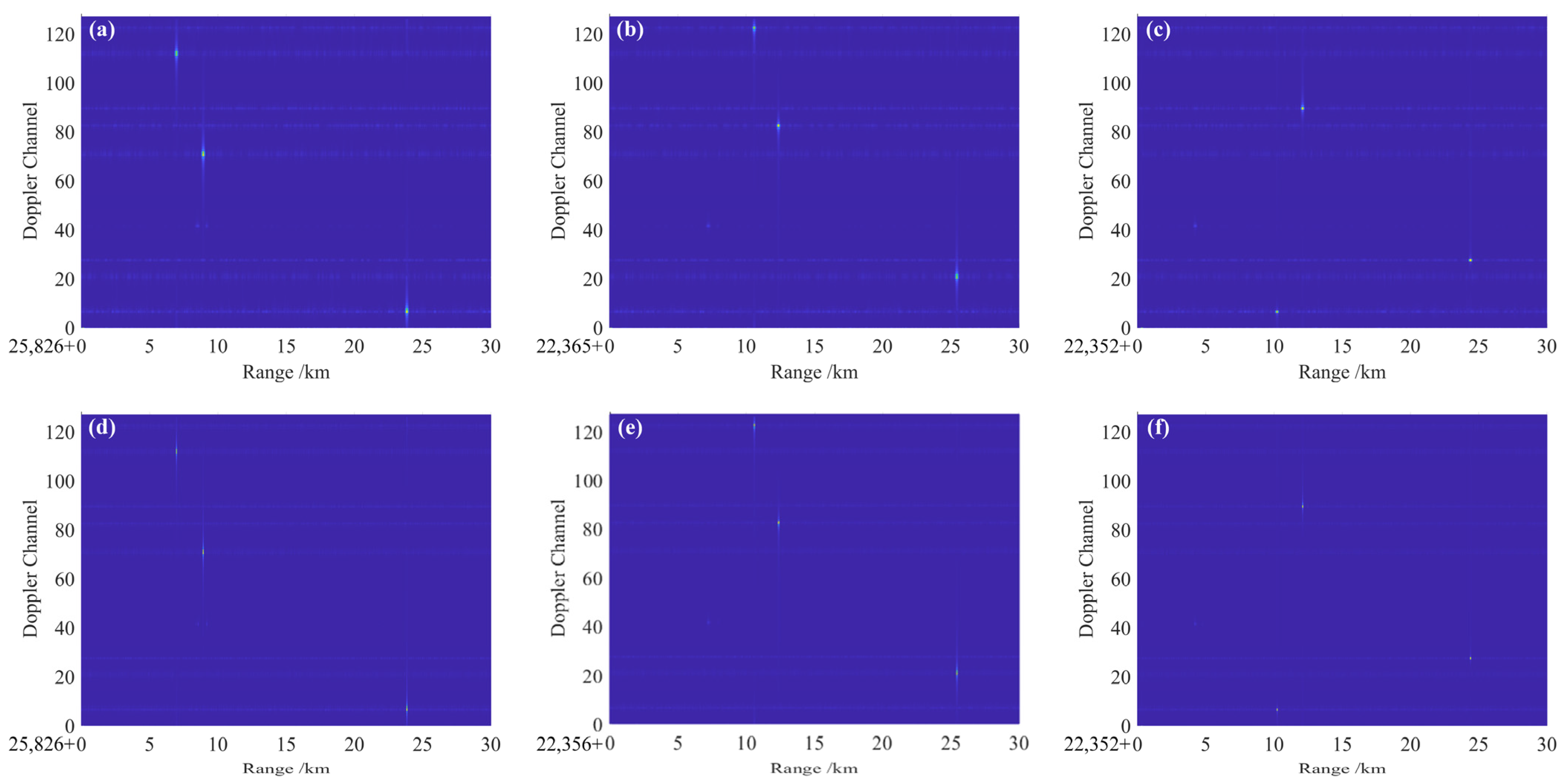
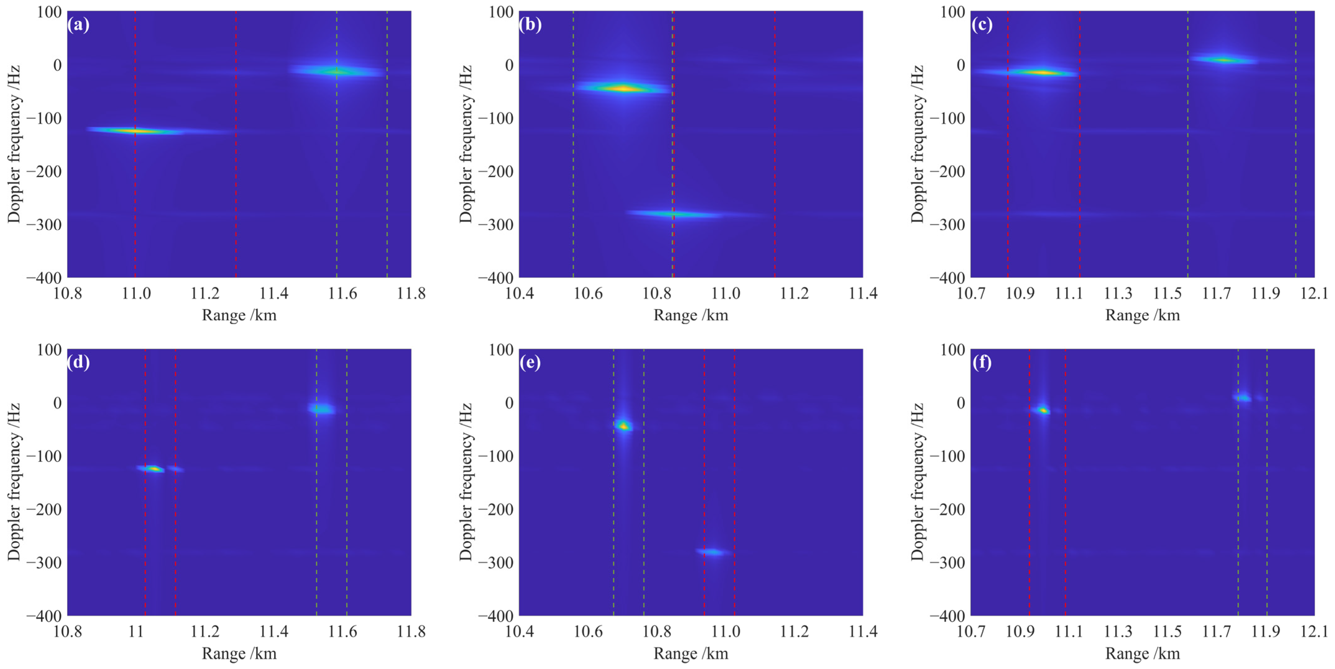
This paper proposes a method for simulating RDM features based on GNSS and an electromagnetic scattering model, enabling the extraction and inversion of characteristic parameters for point targets and ship targets in multi-satellite and multi-target scenarios. Simulation results demonstrate that the GNSS exhibits a strong performance in multi-angle ground detection, with detection ranges reaching meters under the simulation conditions of this study. Moreover, the B3I signal possesses a significant bandwidth advantage over the B1I signal. Under bistatic configurations, the range resolution of the B3I signal reaches the order of tens of meters, whereas that of the B1I signal is at the level of hundreds of meters, significantly enhancing the range resolution capability of the target detection system. The GO-PO method, suitable for electromagnetic calculations of complex targets, is employed to simulate the multiple scattering characteristics of large ship targets on the sea surface. Simulations of RDM using different satellite and signal combinations reveal that the B3I signal accurately reflects the ship’s length information, while the B1I signal exhibits noticeable lateral elongation, resulting in significant deviations in target size and positional information. Therefore, the B3I signal should be prioritized in practical applications; when satellite signal reception power is low or coherent accumulation gain is insufficient, the B1I signal can be utilized as synchronous compensation to improve imaging performance.

Furthermore, this paper introduces the UPF algorithm for the tracking and information inversion of moving targets. Simulation results indicate that the four-satellite system outperforms the three-satellite system under both uniform and accelerated motion scenarios. The positioning error of uniformly moving targets remains stably within 10 m, while that of maneuvering targets is maintained within 18 m; velocity estimation errors are constrained within ±2 m/s, significantly enhancing the system’s dynamic target tracking capability. Multi-satellite, multi-target joint detection not only effectively improves the accuracy of target presence detection but also acquires target distribution information from multiple perspectives. The joint localization approach further refines the estimation of target positions and velocities.

Nevertheless, the low power of GNSS radar signals reaching the ground and the limited signal bandwidth remain critical challenges. The introduction of sparse signal reconstruction techniques holds promise for enhancing detection performance under limited bandwidth or noisy conditions [38,39]. Moreover, we will further incorporate factors such as sea surface conditions and target motion to analyze inversion accuracy and potential improvements under scenarios involving Doppler spread, multipath reflection, or GNSS signal degradation and exploring advanced MIMO radar signal processing methods to develop more effective solutions in subsequent simulation studies.