4.1. Experimental Setup
To validate the effectiveness of the proposed method, we employed both the simulated and measured maritime target datasets, as shown in
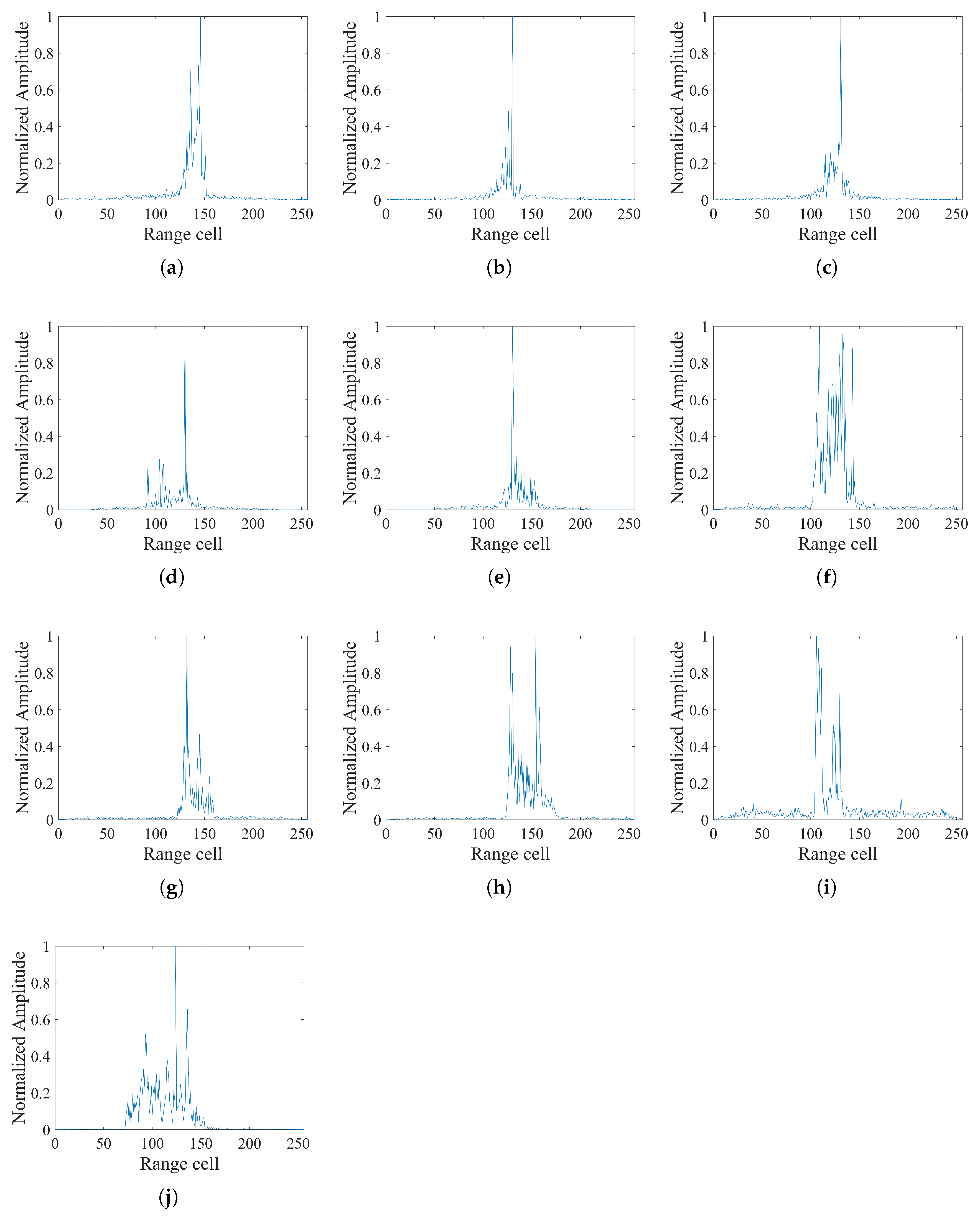
Table 1. The measured dataset was acquired using an X-band phased-array radar system. It comprises ten ship types spanning a size range of 60–250 m, including three cargo ships, three cruise liners, two LNG carriers, and two oil tankers, as shown in
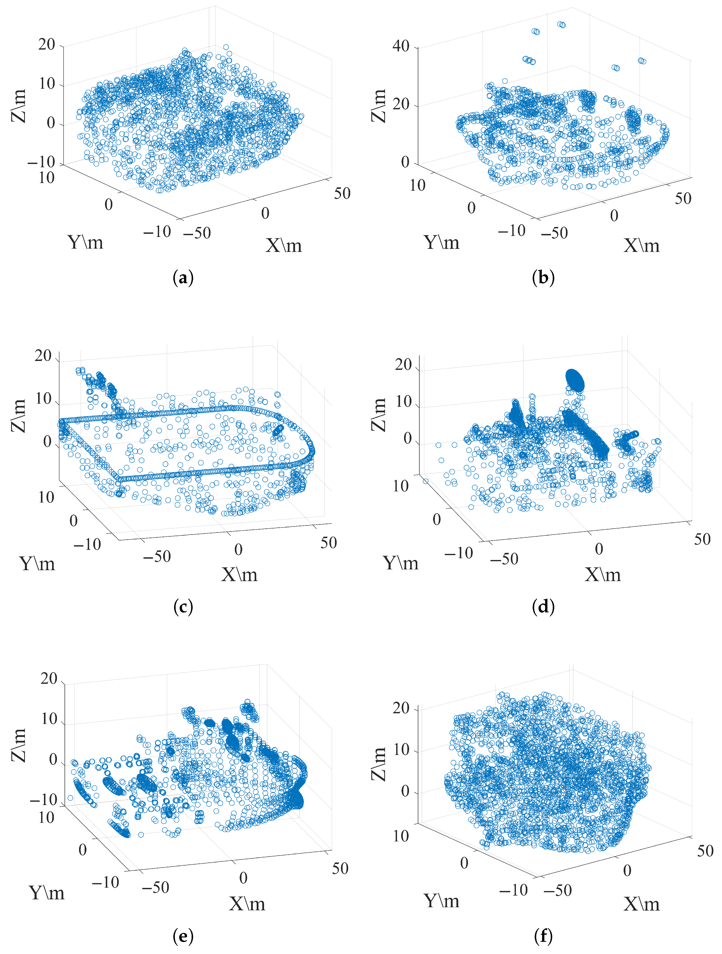
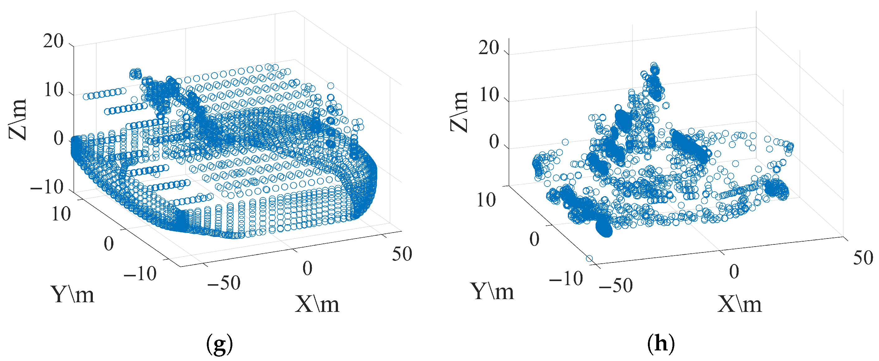
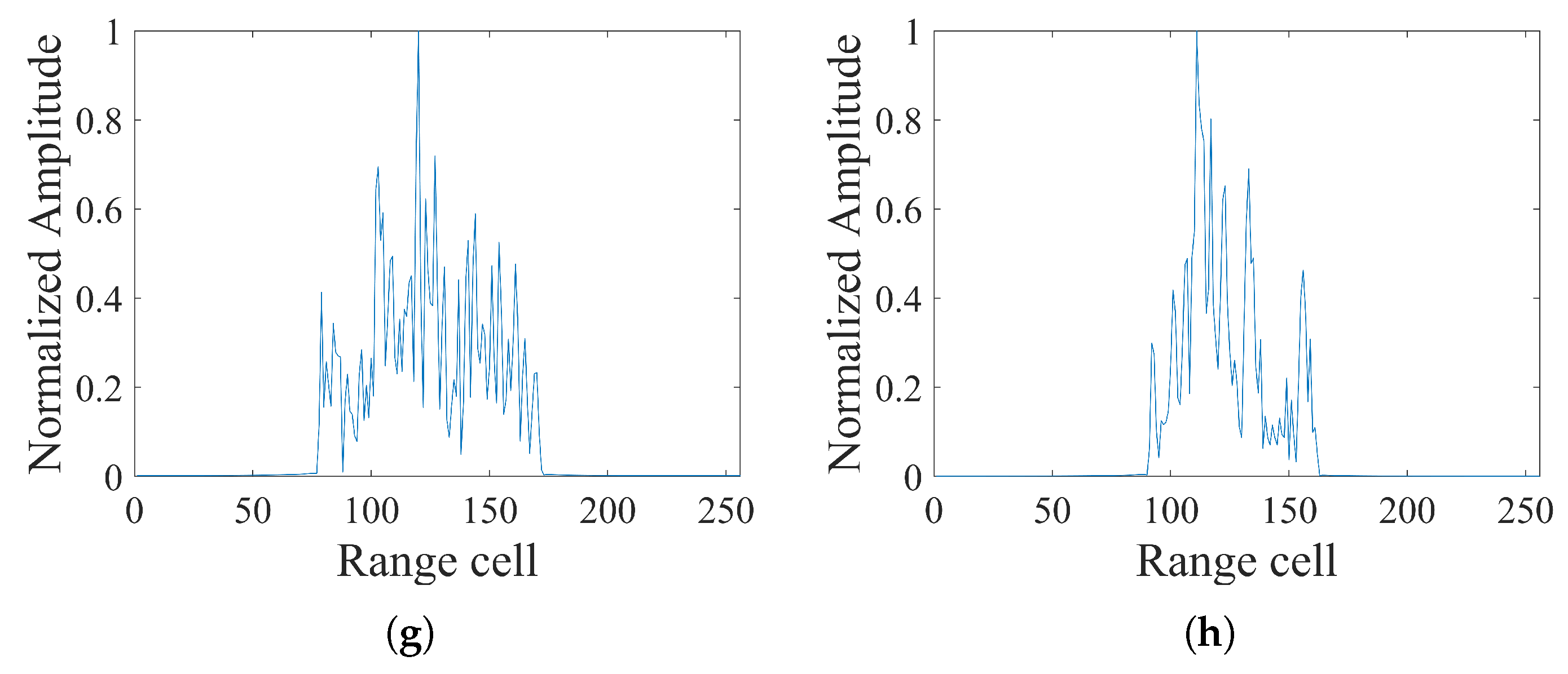
Figure 5. The simulated dataset comprises eight types of ships, as shown in
Figure 6 and
Figure 7. Each class in both datasets comprises 2000 samples. These two datasets were split into training, validation, and test sets with a ratio of 70%, 15%, and 15%, respectively. Additionally, we added 10 dB of white Gaussian noise to ensure generalization.
We implemented our network on a Linux workstation with an Intel Xeon CPU and an NVIDIA RTX 1660s GPU (NVIDIA Corporation, Santa Clara, CA, USA). The network architecture was initialized with an input channel dimension of 8 to align with the inherent dimensionality of HRRP data while maintaining computational efficiency. The hidden dim of the SESF block was set to 16 to optimize the trade-off between feature representation capacity and model complexity.
The initial learning rate was set to 0.0005 and decayed after each epoch with the cosine annealing scheduler. The epoch number was set as 100. The network was trained using the AdamW optimizer with a batch size of 64.
4.2. Experimental Results
To validate the performance of the proposed method, we compare MSDP-Net with ASTT-Net [
21], TACNN-Net [
16], and SA-Net [
19]. The results for both the simulated and measured datasets are presented in
Table 2 and
Table 3, where each experiment was repeated five times to mitigate the randomization in the training process. We employ the accuracy and the
score to evaluate the classification performance. The FLOPs and the number of parameters (Params) are utilized to evaluate the efficiency of each method. The confusion matrices are depicted in
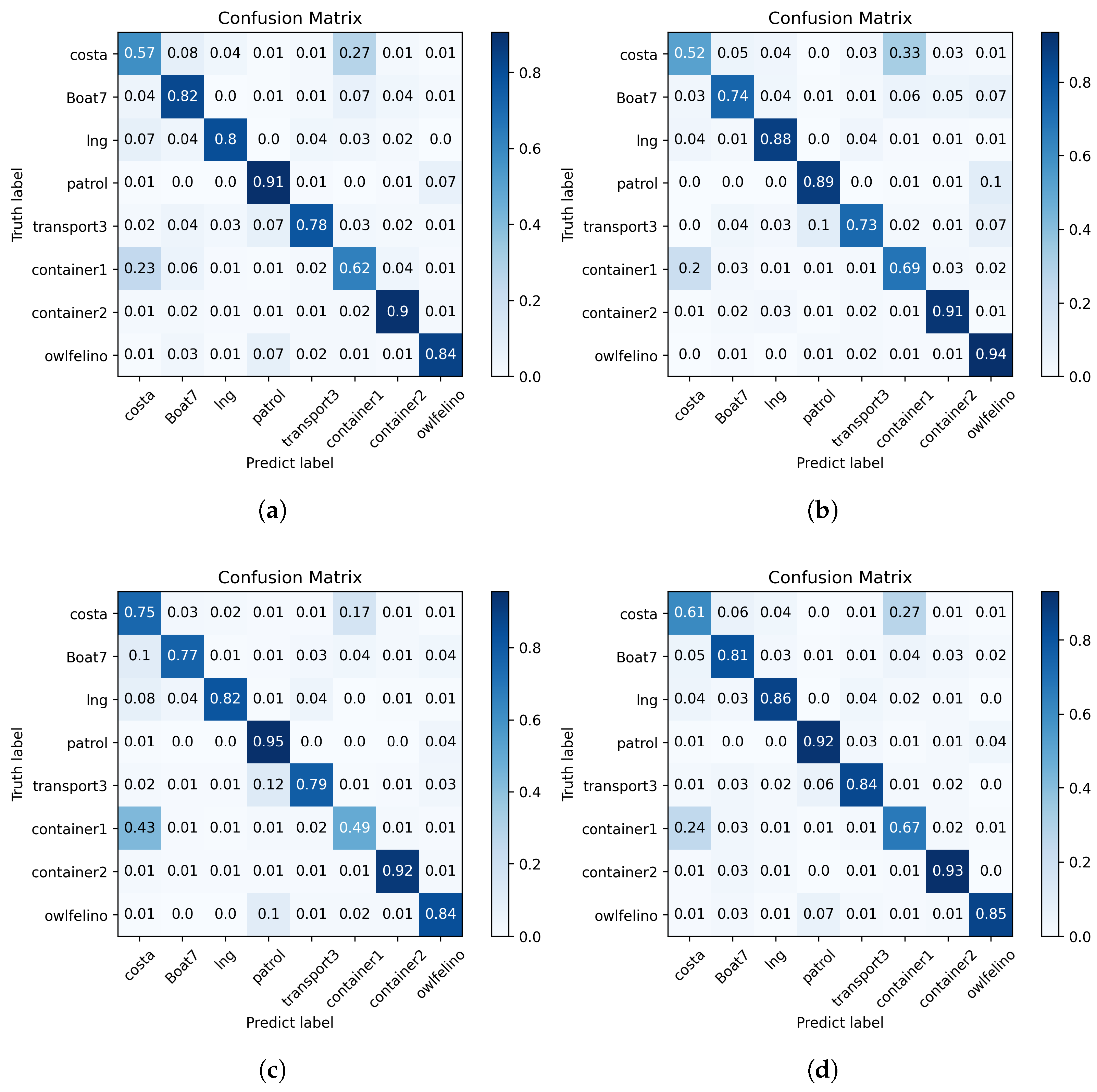
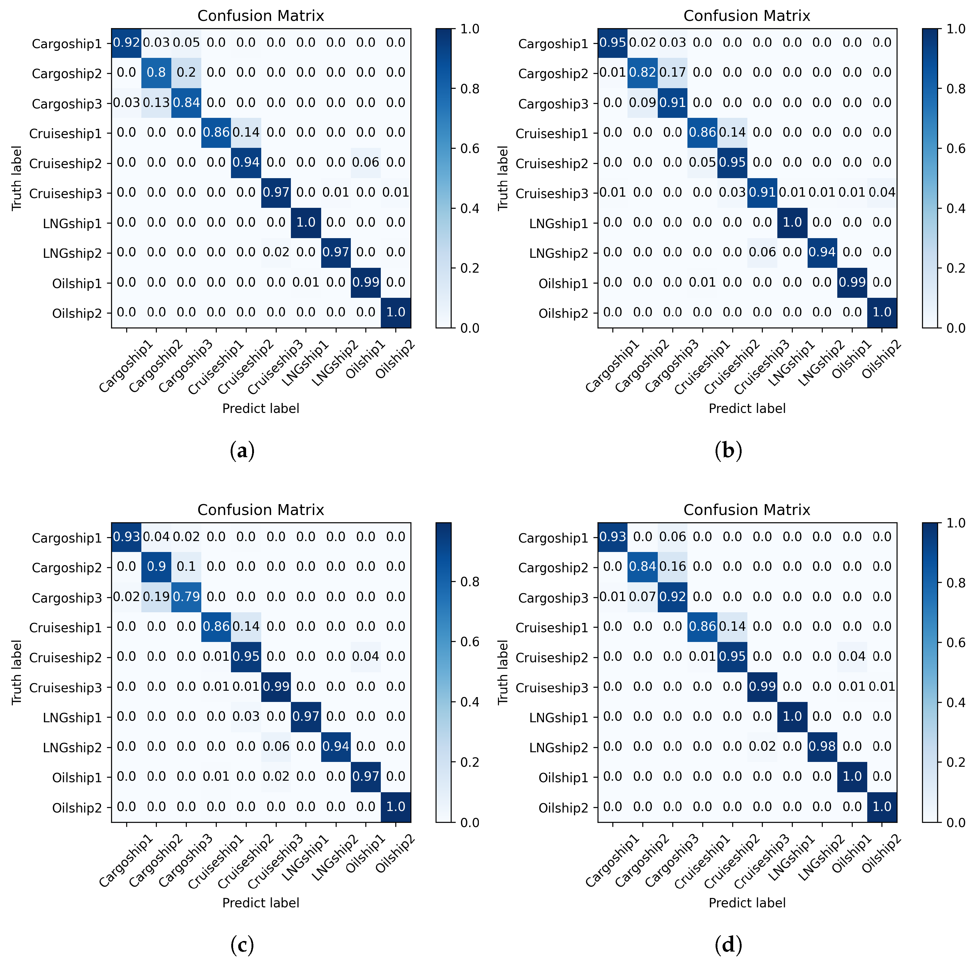
Figure 8 and
Figure 9. We employ accuracy to measure overall correctness across all classes. The
score is utilized to balance precision and recall, which is critical for handling class imbalances. The FLOPs and the number of parameters (Params) are utilized to quantify computational and memory efficiency for practical deployment. The confusion matrices are depicted in
Figure 8 and
Figure 9.
Compared to ASTT-Net, which adopts a discrete wavelet-based swin transformer architecture, MSDP-Net achieves a 2.67% accuracy improvement on the simulated dataset and 2.00% on the measured dataset. This demonstrates the efficacy of integrating the proposed multi-domain perception encoder, which simultaneously captures spatial–spectral interactions that ASTT-Net’s single-domain transformer architecture fails to fully exploit.
When compared with TACNN-Net, which implements attention mechanisms exclusively at the coarsest scale, MSDP-Net exhibits a 1.74% accuracy gain on the simulated data and 1.08% on the measured data. This underscores the advantage of our hierarchical multi-scale feature interaction strategy over TACNN-Net’s scale-restricted attention design, which limits its ability to leverage fine-to-coarse contextual relationships.
Compared to SA-Net, which focuses on spatial structure awareness through conventional convolution blocks, MSDP-Net delivers performance improvements of 1.23% on the simulated dataset and 1.57% on the measured dataset. This validates the necessity of explicitly modeling joint spatial–spectral-domain features through our hybrid encoder, as opposed to SA-Net’s spatial-only feature-encoding paradigm.
These results underscore MSDP-Net’s capacity to facilitate multi-domain feature extraction and exploit complementary information across scales, thereby improving recognition performance.
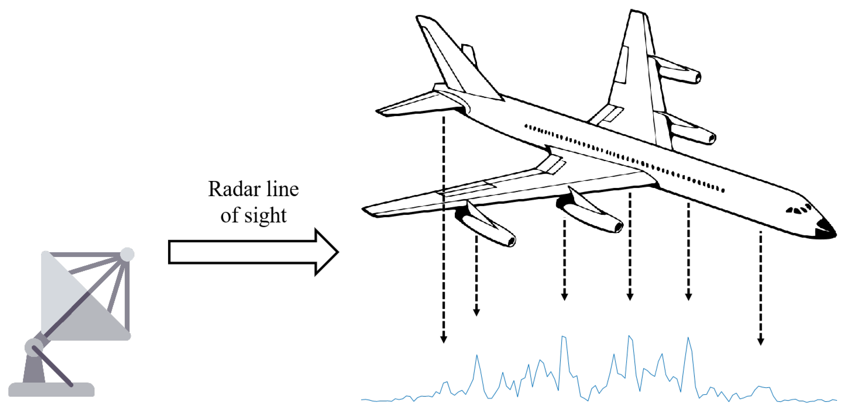
In addition it is observed that our model is generally able to differentiate between the broader categories of Cruiseship and Cargoship. However, confusion mainly arises at the subclass level, such as between Cruiseship1 and Cruiseship2, or between certain Cargoship instances and structurally similar Cruiseships. The difficulty in distinguishing these subclasses lies in the high structural similarity and overlapping scattering characteristics when observed from specific aspect angles. HRRP data represent one-dimensional projections of radar backscattering profiles along the line of sight. As a result, fine-grained structural differences between subclasses may not be sufficiently captured, especially when the aspect angle does not emphasize discriminative features.
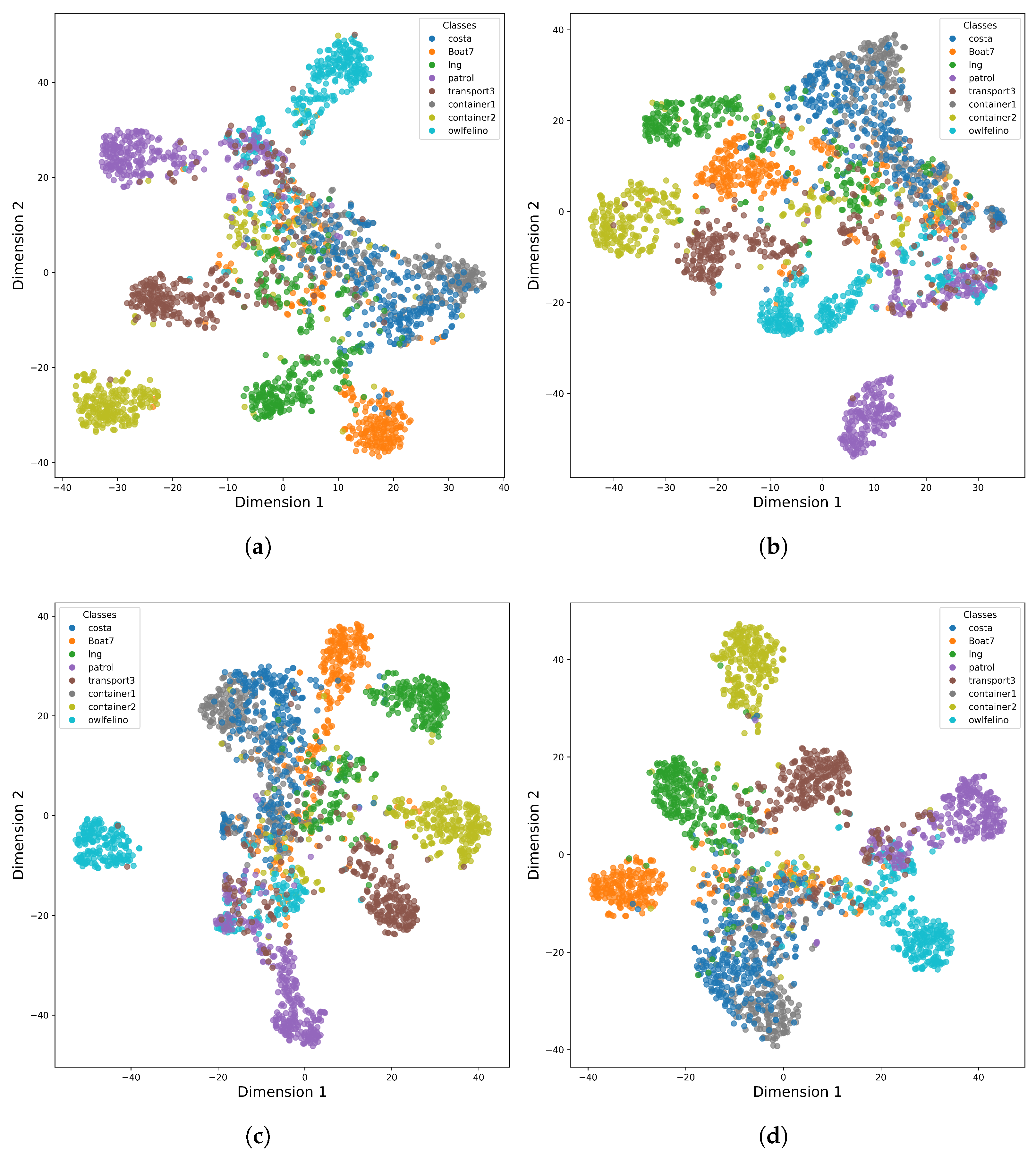
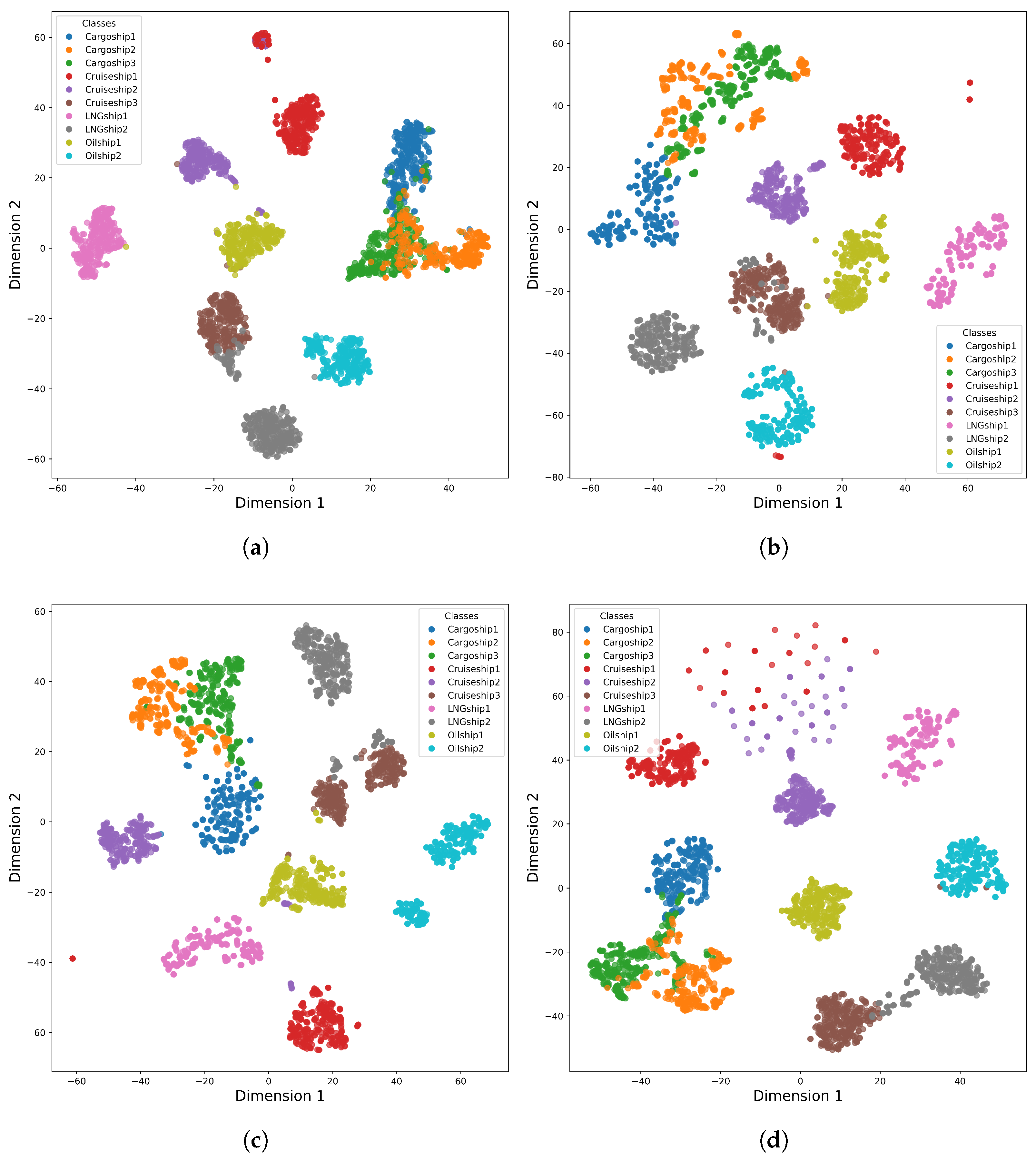
We employ t-SNE [
36], a popular technique for projecting high-dimensional features into a low-dimensional space, to assess how well different approaches separate classes, as shown in
Figure 10 and
Figure 11. Our network’s embeddings form more distinct clusters than those produced by comparative methods. In the simulated dataset, this translates into markedly clearer boundaries between categories, while in the measured dataset we observe substantial gains in the separation of Cargoship1, Cargoship2, and Cargoship3. These figures visually confirm that our architecture yields feature representations with superior discriminative classification.
Moreover, cruise ships and cargo ships often share large, flat surfaces and distributed scattering components, which leads to overlapping patterns in their HRRPs, especially under side-looking or oblique aspect angles. Therefore, all models fail to effectively classify Cruiseship1, Cruiseship2, and Cargoship.
Among the four methods, SA-Net exhibits the smallest parameter count at 0.0602 M, while TACNN-Net and ASTT-Net require 0.2148 M and 0.7764 M parameters, respectively. Our proposed method achieves a parameter budget of 0.1102 M, doubling SA-Net’s parameters but remaining 51% smaller than TACNN-Net and 14% of ASTT-Net’s count, effectively balancing representational capacity with model compactness to reduce storage and transmission overhead.
Considering the FLOPs, the proposed method demonstrates the best computational efficiency with only 4.9 M FLOPs, significantly outperforming ASTT-Net (6.7 M), TACNN-Net (15.6 M), and even SA-Net (6.3 M). Compared to the second-most efficient SA-Net, our method reduces FLOPs by 22%, while achieving a 69% reduction relative to TACNN-Net. This translates to accelerated inference speeds and lower energy consumption under identical hardware constraints.
Furthermore, all methods fail to effectively distinguish between costa and container1, as shown in both the classification results and t-SNE visualization. This is primarily due to the inherent projection characteristics of HRRPs.
An HRRP represents a one-dimensional projection of a target’s scattering centers along the radar LOS, which makes it highly sensitive to the aspect angle of the target. Although costa and container1 are structurally different ships, their backscattering profiles can appear remarkably similar when observed from certain angles. As a result, all models struggle to discriminate between these two classes under specific projection conditions.
4.3. Ablation Studies
To evaluate the contribution of each module, we performed ablation studies on both the simulated and measured datasets. Four variants were analyzed: w/o DP block, w/o SP module, w/o FP module, and w/o HSF branch. We evaluate the performance of these variants and the proposed network utilizing the accuracy,
score, Params, and FLOPs, as shown in
Table 4. The results show that removing the DP block leads to a degradation of 12.74% in the accuracy and 13.17% in the
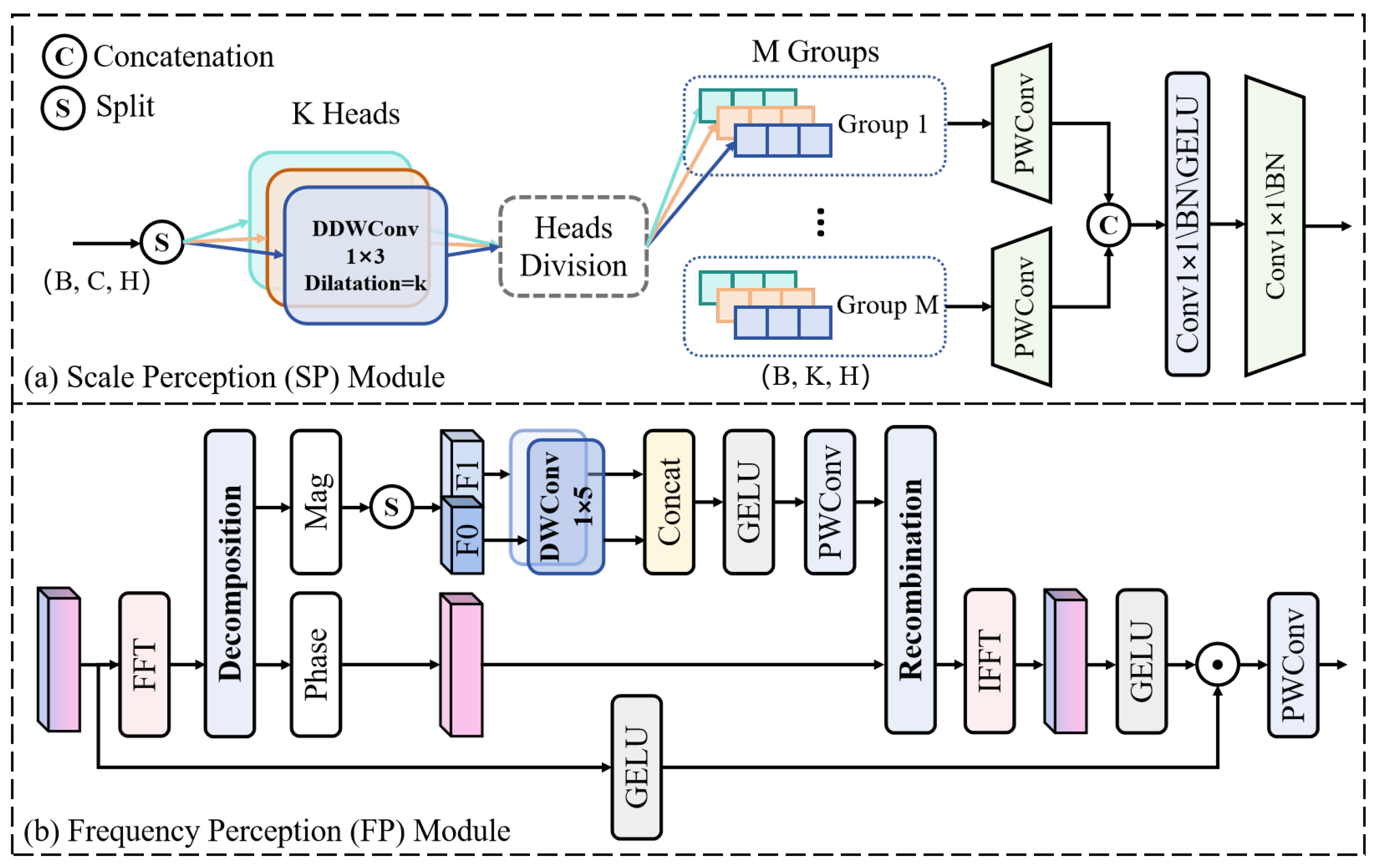
score, demonstrating its role in extracting local and global dependencies. Removing the SP module results in reductions of 2.41% in the accuracy and 2.38% in the
score, indicating the effectiveness of modeling spatial relationships across multiple receptive fields. Removing the FP module causes performance degradations of 0.45% in the accuracy and 0.42% in the
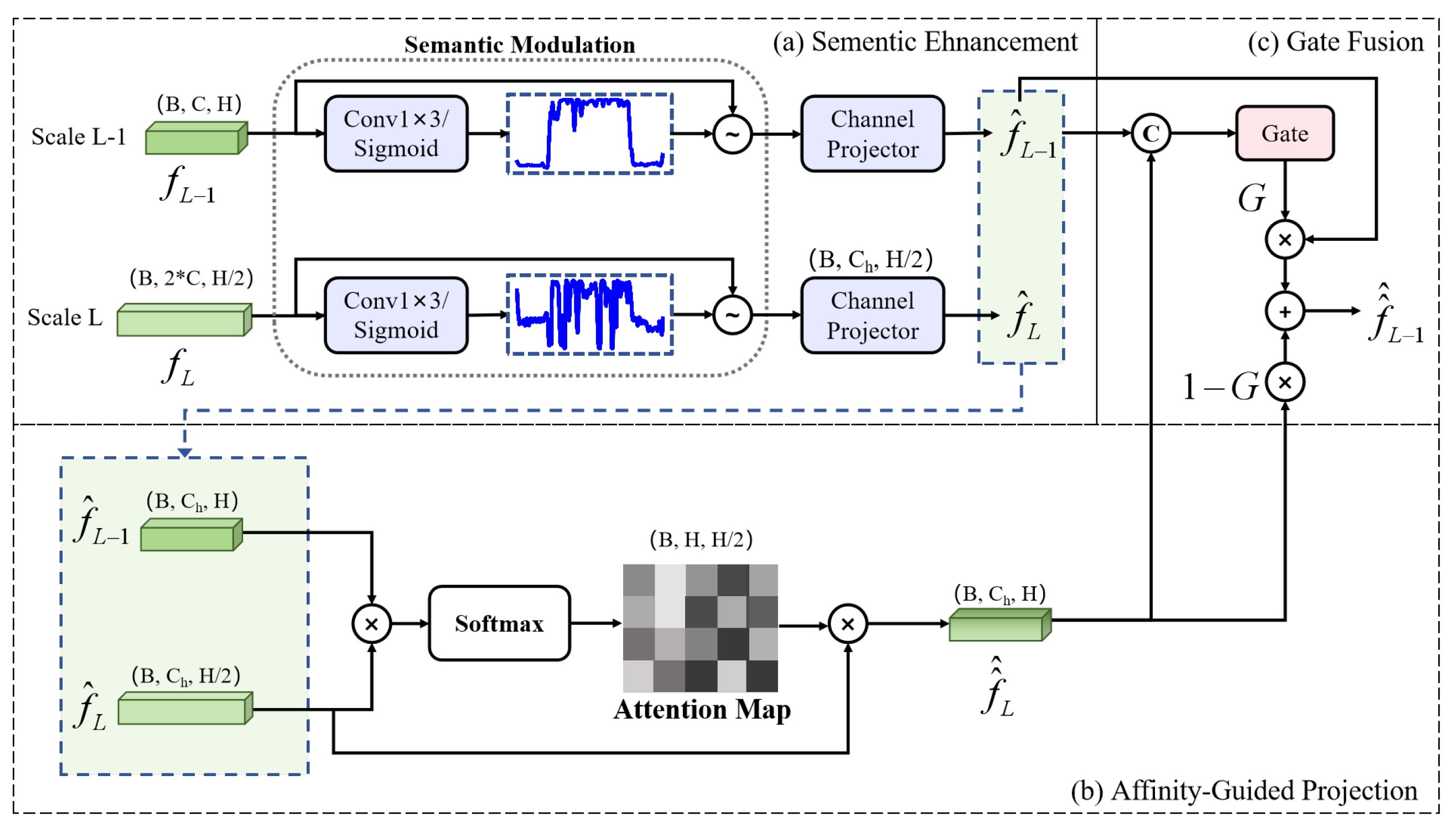
score, showing its ability to capture global spectral dependencies. Removing the HSF branch leads to a degradation of 0.76% in the accuracy and 0.81% in the
score, demonstrating the effectiveness of the bottom-up adaptive scale fusion strategy. These findings demonstrate that combining these modules allows the proposed network to interactively exploit the potential of multi-domain features, achieving improved HRRP target recognition. We also conducted module accumulation experiments, as shown in
Table 5. The results demonstrate that the SP and FP modules significantly improve the model performance with only a small increase in parameters and computational cost.
Considering the computational efficiency, introducing the DP block increases the model size from 0.0353 M to 0.1102 M parameters and raises the FLOPs from 1.8 M to 4.9 M, yet yields the largest performance improvement, which confirms its critical role in joint spatial–spectral modeling. The SP module adds 0.0494 M parameters and 1.9 M FLOPs, while the FP module adds a computational cost of 0.0354 M parameters and 1.8 M FLOPs. Finally, the HSF branch contributes a slight improvement in the computational cost of 0.0023 M parameters and 0.1 M FLOPs. Collectively, these results demonstrate that our architecture allocates computational resources—investing to achieve efficiency and superior recognition performance.


