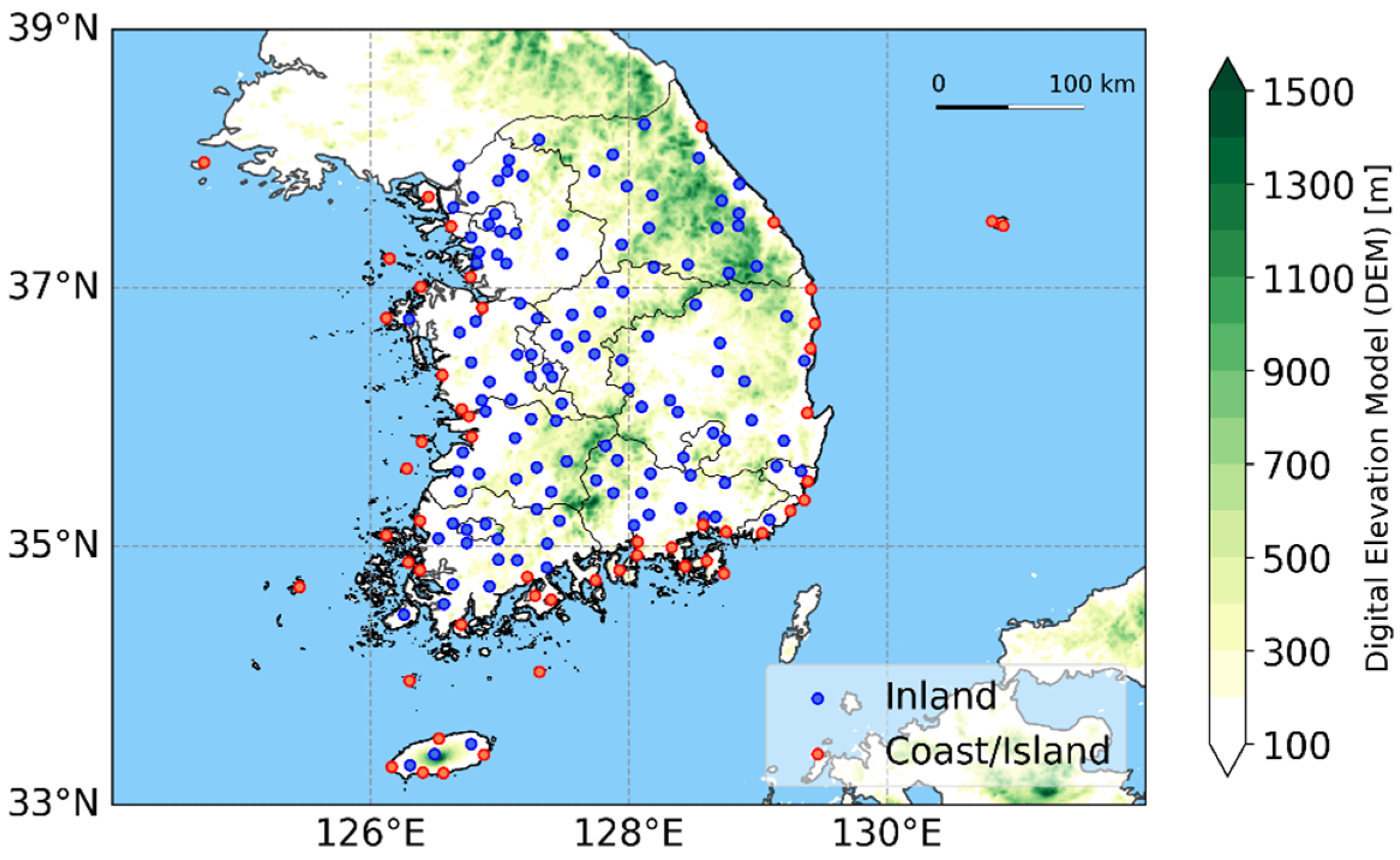
Article

A Detailed Performance Evaluation of the GK2A Fog Detection Algorithm Using Ground-Based Visibility Meter Data (2021–2023, Part I)

by
Hyun-Kyoung Lee
1,2 and
Myoung-Seok Suh
2,*
1
National Meteorological Satellite Center (NMSC), Korea Meteorological Administration (KMA), Guam-gil 64-18, Jincheon-gun 27803, Chungcheongbuk-do, Republic of Korea
2
Department of Atmospheric Science, Kongju National University, 56 Gongjudaehak-ro, Gongju-si 32588, Chungcheongnam-do, Republic of Korea
*
Author to whom correspondence should be addressed.
Remote Sens. 2025, 17(15), 2596; https://doi.org/10.3390/rs17152596
Submission received: 28 May 2025 / Revised: 15 July 2025 / Accepted: 19 July 2025 / Published: 25 July 2025
(This article belongs to the Section Atmospheric Remote Sensing)

Abstract

This study evaluated the performance of the operational GK2A (GEO-KOMPSAT-2A) fog detection algorithm (GK2A_FDA) using ground-based visibility meter data from 176 stations across South Korea from 2021 to 2023. According to the verification method using the nearest pixel and 3 × 3 neighborhood pixel approaches to the visibility meter, the 3-year average probability of detection (POD) is 0.59 and 0.70, the false alarm ratio (FAR) is 0.86 and 0.81, and the bias is 4.25 and 3.73, respectively. POD is highest during daytime (0.72; bias: 7.34), decreases at night (0.57; bias: 3.89), and is lowest at twilight (0.52; bias: 2.36). The seasonal mean POD is 0.65 in winter, 0.61 in spring and autumn, and 0.47 in summer, with August reaching the minimum value, 0.33. While POD is higher in coastal areas than inland areas, inland regions show lower FAR, indicating more stable performance. Over-detections occurred regardless of geographic location and time, mainly due to the misclassification of low-level clouds and cloud edges as fog. Especially after sunrise, the fog dissipated and transformed into low-level clouds. These findings suggest that there are limitations to improving fog detection levels using satellite data alone, especially when the surface is obscured by clouds, indicating the need to utilize other data sources, such as objective ground-based analysis data.

Graphical Abstract

1. Introduction

Fog typically consists of very small, suspended water droplets that reduce horizontal visibility near the surface to below 1000 m. Fog droplet sizes typically range from a few microns up to 20–30 μm, depending on the fog type and environmental conditions. Although fog generally occurs within the boundary layer, its vertical extent can exceed 1000 m under saturated and well-mixed atmospheric conditions [1,2,3,4]. Fog adversely impacts both anthropogenic activities and natural ecosystems. It leads to serious challenges to aviation, maritime, and road transportation safety, degrades air quality, and frequently results in human casualties and economic losses [4,5]. From a climatological perspective, long-term atmospheric changes can influence fog frequency [6,7].
In South Korea, approximately 290 visibility meters operate, observing visibility data at 1 min intervals. The availability of high-resolution spatiotemporal data has facilitated several studies on fog detection and spatial distribution analysis using visibility meter data [8,9,10]. Given the growing need for robust, high-resolution fog detection and forecasting to support transportation safety, recent approaches have increasingly integrated ground-based observations, buoys, and satellite products to analyze and classify fog occurrence [11,12,13,14].
Satellite-based observations provide broad temporal and spatial coverage, enabling continuous monitoring of fog from its formation to dissipation and analysis of its spatial distribution. Before the GK2A(GEO-KOMPSAT-2A) launch, various geostationary and polar-orbiting satellites were used to study fog detection over the Korean Peninsula. Ahn et al. [15] developed an algorithm for detecting oceanic fog and low stratus by comparing hourly infrared radiance data with a clear-sky radiance composite map. Subsequent research utilized GOES (Geostationary Operational Environmental Satellite)-9, COMS (Communication, Ocean, and Meteorological Satellite), Himawari-8, MODIS (Moderate Resolution Imaging Spectroradiometer), and AMSR (Advanced Microwave Scanning Radiometer) data to investigate fog and sea fog characteristics during both day and night [16,17,18,19,20,21,22]. The GK2A fog detection algorithm (GK2A_FDA) constitutes an incremental improvement, incorporating both optical and textural characteristics of fog through additional multiple channels (1.6, 8.7, 10.5, 12.3, and 13.3 µm) from the Advanced Meteorological Imager (AMI).
Nevertheless, satellite-based fog detection remains challenging under a range of observational and atmospheric limitations, including multiple cloud layers obscuring the satellite’s view, subpixel-scale fog, optically thin fog, orographic fog, and low-illumination conditions during the day–night transition period [16,23,24,25]. In addition, low stratus clouds with optical and textural properties similar to fog often lead to false alarms [26,27]. During daytime, cloud shadows and navigation errors can cause an underestimation of the reflectance background field, resulting in the misclassification of low stratus clouds as fog [19,28].
Recent studies have applied data fusion and machine learning techniques to overcome these limitations and enhance satellite-based fog detection. Egli et al. [25] utilized cloud base height data from Meteorological Aviation Routine Weather Reports and Meteosat Second Generation (MSG) satellite imagery to improve fog and low stratus (FLS) detection through a machine learning model. Suh et al. [13] generated high-resolution fog fields by blending GK2A fog detection results with visibility-based objective gridded data, thereby improving detection beneath cloud cover and in regions with limited surface observations. GK2A fog detection also provides a foundation for integrating gridded visibility data and CCTV (closed circuit television)-derived visibility data to support road visibility estimation [14]. An XGBoost-based model was developed to achieve continuous detection of FLS by utilizing both reflectance and brightness temperature channels derived from MSG/SEVIRI (Spinning Enhanced Visible Infrared Imager) [29].
With increasing demand from meteorological forecasting, aviation, maritime, and surface transportation safety, continual improvements to the GK2A_FDA are necessary. Although GK2A fog detection is used operationally, most evaluations have focused on fog events [21,28,30,31]. A comprehensive performance evaluation using year-round data has become imperative to ensure the robustness of the GK2A_FDA.
Considering surface background types, regional variations in fog characteristics across South Korea, and time-dependent differences in satellite channel usage, the GK2A_FDA is divided into nine sub-algorithms based on region (inland, coast, and ocean) and time of day (daytime, twilight, and nighttime) [20,28,31]. This study presents detailed statistical analysis and case studies of six sub-algorithms—daytime, nighttime, and twilight algorithms for both inland and coastal regions—that can be evaluated using ground-based visibility observations. The ocean algorithms are excluded from this analysis due to the lack of ground-based validation data over ocean areas. The results provide a foundation for future improvements. Section 2 describes the data and methodology; Section 3 presents performance evaluation and case studies; Section 4 provides a general discussion including improvement strategies; and Section 5 summarizes the conclusions.

2. Materials and Methods

2.1. Data

The study area, as shown in Figure 1, covers inland and coastal regions of South Korea, where the evaluation of the GK2A_FDA is feasible using ground-based visibility meters. The domain also includes several islands. The study period spans three years, from 2021 to 2023. A quantitative evaluation was conducted using GK2A fog detection products at 10 min intervals with visibility meter data. Subsequently, case studies were performed using supplementary datasets, including cloud top height from GK2A, low-level cloud base height from ceilometers, and meteorological variables such as temperature, relative humidity (RH), and wind speed from ASOS (Automated Synoptic Observing System) and AWS (Automated Weather System) stations (Table 1).

2.1.1. GK2A Fog Product

The GK2A satellite, a geostationary meteorological satellite launched in December 2018, is equipped with the AMI, which includes 16 channels covering visible, near-infrared, and infrared wavelengths. The GK2A_FDA utilizes full-disk observations at 10 min intervals, from which the Korean Peninsula domain is extracted. Inputs include radiance from 8 channels, such as the 0.64 µm visible reflectance, 3.8 µm shortwave infrared, and 11.2 µm infrared window brightness temperatures (BT), as well as auxiliary variables such as solar zenith angle (SZA), clear-sky radiance (CSR) at 11.2 µm, land-sea mask data, and prior fog detection results [20,28].
As illustrated in Figure 2, the algorithm comprises nine sub-algorithms and a post-processing step structured by geographic region and time of day. Each sub-algorithm is implemented using a decision tree method. Inland and coastal pixels are classified into three categories (daytime, twilight, and nighttime) based on SZA.
For daytime pixels, twelve sequential tests are conducted. These include the difference between normalized 0.64 μm reflectance and its surface reflectance background at 0.64 μm (ΔVIS0.64 μm); the fog-top to modeled surface temperature difference, calculated as CSR_BT11.2 μm−BT11.2 μm (ΔFTs); the normalized local standard deviation (NLSD) applied for texture analysis to differentiate fog from both clouds and cloud edges; and the normalized difference snow index (NDSI). Furthermore, a fog lifecycle constraint is applied for SZA ≤ 60° to prevent new fog detections, based on comparisons with the previous time step. In inland areas, stricter thresholds for ΔVIS, ΔFTs, and NLSD 0.64 μm are applied to improve discrimination between fog and low stratus clouds.
At night, the algorithm applies five decision rules. These include the dual-channel brightness temperature difference (DCD = BT3.8 μmBT11.2 μm), ΔFTs, and the local standard deviation at 11.2 μm (LSD11.2 μm). To minimize temporal discontinuities, the algorithm also incorporates the previous fog detection results for the twilight period. In addition, it performs a three-step procedure that identifies newly formed fog or removes clouds by applying more stringent thresholds. These thresholds were initially determined through histogram analysis of selected fog cases and subsequently optimized by maximizing the Hanssen–Kuiper Skill Score (KSS) [28].
In coastal regions, the algorithm ensures spatial continuity with inland areas by simultaneously applying both inland and ocean fog detection algorithms through a spatial blending approach. A pixel is classified as fog if both algorithms detect fog, or if one detects fog, at least five out of the 3 × 3 neighboring pixels are also classified as fog.
The final GK2A fog product classifies each pixel as fog, clear, cloud, snow, or unknown (Table 2) and provides a quality flag indicating data availability and reliability. The GK2A fog detection product, including pixel-level fog classification, ΔFTs, and quality flags at a spatial resolution of 2 km, is provided every 10 min for both the East Asia and Korean Peninsula domains.
Further details on the algorithm design and threshold settings are described in [20,28]. The land-sea mask used in the GK2A fog detection product also has a 2 km resolution and classifies each pixel as inland, ocean, or coastal. Coastal pixels are defined as those adjacent to the coastline within a 3 × 3 neighborhood.

2.1.2. Ground-Based Observations

Visibility meters estimate visibility (in meters) by measuring the intensity of light scattered and absorbed as a laser beam passes through the atmosphere. Each minute, the instrument produces a visibility value based on multiple measurements sampled at 15 to 30 s intervals. The 10 min moving average of these values is used as the current visibility reading [32].
Ground-based visibility data were obtained from 176 stations selected for their relatively high data quality, as identified by the National Meteorological Satellite Center (NMSC). Based on the land-sea mask (lsmask) in the GK2A fog detection product, 124 stations were categorized as inland and 52 as coastal, including island stations (Figure 1). A fog event was defined when the observed visibility was less than 1 km, and the RH measured by co-located ASOS or AWS instruments was equal to or greater than 88% [30].
For the case studies, ground-based observations from ASOS were used, including surface air temperature, RH, and wind speed. The vertical structure and depth of fog were investigated by utilizing low-level cloud base height derived from ceilometers and cloud top height data from GK2A.

2.2. Methodology

2.2.1. Temporal and Spatial Collocation

Temporal consistency between GK2A satellite observations and ground-based visibility measurements was ensured by synchronizing the visibility data using the median of five 1 min interval values collected between min 00 and 04 past the hour. This method accounts for the delay of approximately 2–3 min in GK2A observations over the Korean Peninsula following the start of each full-disk scan cycle.
Spatial colocation was achieved by extracting GK2A fog detection values from the satellite pixel nearest to each visibility meter site. Fog detection results from a 3 × 3 pixel neighborhood centered on the nearest pixel (i.e., the 3 × 3 neighborhood pixel method) were also utilized to compensate for potential satellite geolocation errors and to improve spatial representativeness by accounting for local variability around the observation site.

2.2.2. Evaluation Method

The detection performance of the GK2A_FDA was statistically evaluated using a 2 × 2 contingency table (Table 3). A satellite detection was considered a hit (H) if fog was detected by GK2A and observed at the ground station. A false alarm (F) was recorded when fog was detected by the satellite but not by the visibility meter, while a miss (M) indicated fog observed by the visibility meter but not detected by the satellite. A correct negative (C) was recorded when both the satellite and the visibility meter indicated no fog. The evaluation was performed using both the nearest GK2A pixel and the 3 × 3 neighborhood pixel methods [31].
The performance of the GK2A_FDA was evaluated using three widely adopted categorical verification metrics: the probability of detection (POD), false alarm ratio (FAR), and bias. Their formulas are provided in Equations (1)–(3):
POD = H/(H + M),
FAR = F/(H + F),
Bias = (H + F)/(H + M)
POD indicates the probability of correct fog detection, with values closer to 1 representing higher hit rates. FAR reflects the probability of false detection, with values near 1 indicating higher false alarm rates. Bias measures the tendency of the algorithm to overestimate or underestimate fog occurrence; values above 1 indicate over-detection, while values below 1 indicate under-detection.

2.2.3. Data Selection

The spatial classification used to evaluate the GK2A fog detection performance over inland and coastal regions was based on the lsmask provided in the GK2A fog product. The temporal classification was determined by SZA at each pixel: SZA < 80° was considered daytime, 80° ≤ SZA < 88° twilight, and SZA ≥ 88° nighttime.
As shown in Table 4, Flag 0 represents nominal data with complete channel availability and valid detection. Flags 1 to 13 indicate cases of partial input data loss or invalid prior detection data [28]. Flag 15 (mid- to high-level clouds) accounted for 43.34%, while Flag 14 (snow contamination) accounted for 3.73%. Pixels affected by clouds or snow cover were excluded from the evaluation to ensure reliable fog/no fog classification based on the quality flags and product values (see Table 2), as these conditions often prevent accurate satellite observation [25,29].
In this study, six sub-algorithms excluding the ocean category were evaluated using available ground-based validation data. Moreover, fog performance was evaluated on a monthly basis to account for the seasonal variability in fog occurrence. A total of 156,369 scenes (99.2%) were used in the analysis out of a theoretical maximum of 157,680 scenes (3 years × 365 days/year × 24 h/day × 6 scenes/h), excluding scenes with missing data due to operational issues.

3. Results

3.1. Quantitative Evaluation of Fog Detection

3.1.1. Overall Fog Detection Performance

Figure 3 presents the seasonal frequency of annual average fog observations at 176 visibility meter stations used to validate the GK2A_FDA. Depending on the season and location, the number of foggy days shows substantial spatiotemporal variability, ranging from 0 to approximately 40 days. Along the west coast, fog occurrences are most frequent during spring and summer, whereas in inland regions, they are more prominent in autumn [33,34,35]. In contrast, the east coast exhibits a lower overall frequency of fog and, at specific stations, no ground-based fog observations during the winter season [12,35].
The evaluation using the nearest-pixel method yielded a three-year average POD of 0.59, a FAR of 0.86, and a bias of 4.25. In contrast, the evaluation based on the neighborhood pixel led to improved detection performance, with a POD of 0.70, FAR of 0.81, and Bias of 3.73. Year-to-year variation in the metrics was relatively small, although 2022 showed a slightly higher bias (Table 5).
Regardless of the validation method, the POD of the GK2A_FDA was generally acceptable in the context of satellite fog detection, indicating a reasonable fog detection rate. However, the relatively high FAR and bias values suggest a tendency toward over-detection. To more conservatively assess the detection performance, this study primarily applied the nearest-pixel approach rather than the 3 × 3 neighborhood pixel method. Therefore, the fog detection performance presented in this study reflects a minimum estimate rather than the maximum potential capability of the GK2A_FDA.

3.1.2. Fog Detection Performance by Algorithm

The fog detection results of the GK2A_FDA validated by the nearest pixel approach, based on geographic location and time, are summarized in Table 6. The detection performance of GK2A_FDA varied substantially depending on geographic location and time of day across all evaluation metrics.
Inland regions showed a lower POD of 0.57 compared to 0.67 for coastal regions; Nonetheless, the bias was also relatively lower at 4.00 versus 5.26, indicating a more stable detection performance with reduced overestimation. The POD across different time zones ranged from 0.51 to 0.83, showing moderate to good performance in daytime > nighttime > twilight. In contrast, the FAR ranged from 0.77 to 0.93 and the bias from 2.21 to 11.93, demonstrating a general tendency toward over-detection, with significant variability in bias depending on region and time. Both inland and coastal areas maintained relatively stable detection performance during nighttime, exhibiting similar bias values.
In daytime conditions, by contrast, the bias increased markedly—reaching 11.93 in coastal areas and 6.12 in inland areas—indicating a strong over-detection tendency, particularly along the coast. This over-detection is associated with a structural characteristic of the GK2A_FDA as applied to coastal regions, where using both inland and ocean fog detection algorithms tends to result in higher FAR and bias during daytime. The daytime period corresponds to the dissipation stage of the fog lifecycle, during which fog dissipates from the surface [36,37,38] and may appear as low-level stratus clouds at ground level [39]. Nonetheless, satellites are likely to detect such conditions as fog, increasing the likelihood of false alarms [19,31].
In inland areas during the daytime, the GK2A_FDA tends to misclassify low-level clouds as fog due to errors in the numerically modeled clear-sky surface radiance used for ΔFTs calculation [31]. In ocean regions, the less stringent ΔFTs threshold, introduced to enhance the detection of rapidly developing sea fog over the Bohai Sea, increases the risk of misclassifying low stratus or dissipating fog as fog [20,40].
Fog detection in coastal areas is based on the combined results of both inland and ocean algorithms (Figure 2). If either algorithm detects fog, and five or more of the adjacent 3 × 3 pixels are identified as fog, the target pixel is also classified as fog. This process aims to improve the fog detection levels and enhance the spatial continuity of coastal areas, which not only have the characteristics of inland and oceanic background environments but also possess unique fog occurrence characteristics. The considerable bias value during the day in coastal areas can be attributed to a combination of the following factors: (1) a relatively small number of validation points and a low frequency of fog occurrence, (2) the conservative fusion of detection results from applying both inland and ocean fog detection algorithms simultaneously to enhance spatial continuity, and (3) the misdetection of fog that dissipated after sunrise, as seen inland (Figure 2).
The over-detection tendency is consistent with the study of Han et al. [31], which highlighted the need to refine the daytime fog detection algorithm to address issues such as satellite navigation errors, cloud shadow contamination, and uncertainty in the clear-sky reflectance composite. The findings indicate that further algorithmic sophistication and improved post-processing are necessary to enhance the performance of the GK2A daytime algorithm.
Figure 4 presents the GK2A_FDA’s monthly and seasonal fog detection performance, categorized by region and time. The quantitative detection statistics are summarized in Appendix A, Table A1, Table A2, Table A3 and Table A4.
The monthly average POD in inland areas ranges from 0.33 (all day, August) to 0.74 (all day, January), representing the lowest and highest values observed during summer and winter, respectively (Figure 4d). Notably, during daytime, POD maintains relatively stable and high values between 0.65 and 0.74, outperforming other periods (Figure 4a). In contrast, both FAR and bias remain high throughout most of the year, except autumn, as indicated by their monthly averages ranging from 0.70 to 0.95 and 2.08 to 9.68, respectively (Figure 4d).
During nighttime, the seasonal POD reaches its maximum in winter, remains moderate in spring and autumn, and declines substantially in summer (Figure 4b), a pattern consistent with the seasonal variation in nighttime fog and low cloud detection accuracy using the Day/Night Band and infrared channels of S-NPP/VIIRS (Suomi National Polar-orbiting Partnership/Visible Infrared Imaging Radiometer Suite), with missed detections and false alarms predominantly occurring at cloud edges due to parallax effects and temporal mismatches between satellite and ground observations [41]. The monthly bias values are more stable than those in coastal regions but show peaks in January and June. Although twilight yields the lowest POD among all-time categories, they are associated with relatively lower FAR and bias values, suggesting more conservative detection behavior in that period (Figure 4c).
Although the monthly daytime POD in coastal regions is less stable than in inland areas, it generally shows superior performance, except in August (Figure 4e). However, FAR and bias are also higher, indicating a clear tendency toward over-detection. During nighttime, the POD gradually decreases from winter to spring, summer, and autumn. The FAR remains high during the night and reaches its maximum in August, while the bias attains its highest value in winter (Figure 4f). Similar to inland conditions, twilight periods exhibit relatively lower FAR and bias values (Figure 4g).
Wærsted et al. [42] reported that higher air temperatures can reduce the efficiency of radiative cooling near the surface, thereby making fog formation and maintenance more difficult or leading to its rapid dissipation. August on the Korean Peninsula is influenced by the East Asian monsoon and is characterized by the highest monthly average air temperatures [43]. During this month, the daily mean sea surface temperatures (SSTs) are often comparable to, or even exceed, the air temperatures [33]. Moreover, coastal regions are frequently affected by convective and multilayered cloud development. As a result, the quality of the 30-day minimum value composition of visible channel reflectance is often degraded, making it more challenging to distinguish between fog and low-level clouds. Consequently, when fog occurrence substantially decreases in coastal areas in August, POD values are the lowest, while FAR and bias values are the highest (Figure 4h), a tendency that is also observed in inland regions. In contrast, January exhibits high POD values. Nonetheless, FAR and bias also remain high, likely due to the influence of low stratiform clouds forming under stable atmospheric conditions [44].
Table 7 summarizes seasonal detection performance. The seasonal POD reaches its maximum in winter, remains moderate in spring and autumn, and declines substantially in summer (0.47–0.65). Although FAR remains generally high across all seasons (0.75–0.93), it is lowest in autumn and highest in summer. Bias shows a marked tendency toward over-detection, with values of 6.44 in summer and 6.43 in winter, compared to a significantly lower value of 2.48 in autumn.

3.1.3. Fog Detection Performance by Solar Zenith Angle

Figure 5 illustrates the annual mean fog detection frequency of the GK2A_FDA and surface-based fog observations, stratified by SZA in 4° intervals. The distribution of monthly SZA varies seasonally, with smaller values in summer and larger values in winter due to the Earth’s axial tilt. The GK2A_FDA generally reports higher fog detection frequencies than surface observations. Under nighttime conditions, however, the two distributions converge, indicating relatively stable detection performance without solar radiation. Previous studies [41,45] have shown that nighttime fog detection algorithms—which rely primarily on infrared brightness temperature differences such as DCD—tend to yield lower POD than daytime algorithms that utilize visible channels. However, these nighttime algorithms also result in lower FAR and bias values, indicating a relatively reduced rate of false or over-detections under nighttime conditions compared to daytime scenes.
Detection performance tends to degrade during twilight, making fixed threshold-based approaches, typically applied during daytime or nighttime, less effective. Thus, the GK2A_FDA relies mainly on fog detection outcomes from the preceding observation, and while twilight POD is relatively lower than during daytime or nighttime, the corresponding FAR and bias values are also lower. Seasonal changes in the SZA, notably the transition from winter to summer, combined with cloud shadows and navigation errors, degrade the quality of the 30-day minimum value composition of visible channel reflectance during daytime [31]. This degradation leads to false detection of clear-sky regions as fog when the daytime algorithm is applied over inland areas and causes discontinuities in detection results with twilight conditions. The discontinuities in fog detection become most pronounced in June when SZA reaches its annual minimum. This pattern is clearly illustrated in the spring and early summer graphs in Figure 5, where bias increases and the GK2A fog detection frequency rises sharply as the SZA drops below 80°. At SZA values below 60°, most fog has dissipated, resulting in very low ground-based fog occurrence [11,12]. During this low-SZA period, although the GK2A daytime algorithm applies stricter thresholds, Bias still tends to increase noticeably as the SZA decreases.

3.1.4. Fog Detection Performance at Visibility Meter Stations

Figure 6 presents the seasonal distribution characteristics of POD, FAR, and Bias for GK2A_FDA at 176 individual visibility meter stations by the nearest pixel approach. As indicated by the seasonal frequencies for each site shown in the figure, stations with high POD values (top 25%, POD ≥ 0.78) are most frequently located over inland regions during winter, followed by coastal regions in spring and inland regions in autumn, while they are least frequent in summer (Figure 6a). Stations with low POD values (bottom 25%) show an opposite tendency, predominantly concentrated over inland areas in summer and distributed along the east and south coasts during autumn (Figure 6b). Figure 6c,d show the top and bottom 25% distributions of FAR. Stations with low FAR values (top 25%) are concentrated mainly in autumn, whereas those with high FAR values (bottom 25%) appear most frequently in summer, followed by winter, autumn, and spring. The spatial pattern of bias closely resembles that of FAR. Stations with low bias values (top 25%) are primarily concentrated over inland areas in autumn, while stations with high bias values (bottom 25%) occur most frequently in summer (Figure 6e,f).

3.2. Case Studies of Fog Detection

3.2.1. High-Performing Cases

Figure 7 presents time series of visibility, meteorological variables, and GK2A_FDA results at Suwon from 15:00 LST (UTC = LST–9 h) on 28 September to 15:00 on 29 September 2022, depicting fog development and the performance of the satellite detection algorithm. Here, LST refers to Local Standard Time, and UTC stands for Coordinated Universal Time. After sunset on the 28th, favorable conditions for radiation fog formation developed, with clear skies, light winds, and increasing RH due to radiative cooling [4,37]. The surface temperature dropped below the air temperature starting from 17:00 and remained lower until fog onset. GK2A_FDA detected the fog from 02:30 (using the nearest pixel method) and from 02:00 (using the 3 × 3 adjacent pixel method) until 09:00 in both cases (Figure 7a). Visibility meter data indicated fog from 02:20 to 06:50.
At the same time, human visual observations reported fog from 02:15 to 07:10. After sunrise, visibility significantly improved. Both the lower cloud base height and the GK2A cloud-top height (CTH) increased (Figure 7b), indicating a transition from fog to low stratus. Nevertheless, the GK2A_FDA continued to detect fog for approximately two additional hours. Around 09:00 on the 29th, the satellite detection status changed to ‘unknown,’ reflecting a condition where only some fog detection thresholds were satisfied.
This case demonstrates the stable nighttime performance of the GK2A_FDA in detecting radiation fog while also highlighting a limitation during fog dissipation, in which residual low-level clouds are misclassified as fog due to lingering radiative conditions after sunrise.
Fog detection performance corresponding to each image in the time series shown in Figure 7 is summarized in Table 8. The results indicate that the initially high accuracy during the fog development phase significantly declined during the dissipation phase, as reflected by a decrease in POD and increases in both FAR and bias. This pattern demonstrates the algorithm’s tendency to over-detect fog when low-stratus clouds persist after fog dissipation.

3.2.2. Low-Performing Cases

On the night of 20 January 2021, warm air advected from the Yellow Sea by southwesterly to west-southwesterly winds ascended as it converged with a temperature trough over the Korean Peninsula. During this ascent, adiabatic cooling led to condensation of saturated air, forming widespread low-level clouds over the west coast and inland regions. From 21:00 on 20 January to 05:00 the following morning, the GK2A_FDA falsely detected these low-level clouds over the western region as fog (Figure 8a,b).
Ground-based visibility meters reported no fog, while ceilometer data showed cloud base heights between 1.0 and 1.5 km (Figure 8b,c). This case represents a typical example of false fog detection during winter when stratiform low clouds frequently develop over the western Korean Peninsula. The GK2A CTH was estimated at approximately 2.5 km at night and around 1 km after 07:00 the next morning (Figure 8c). Surface RH remained consistently low at around 40%, with only minor fluctuations during the event, and air temperature, after decreasing following sunset, gradually increased once the low clouds were observed, indicating thermodynamic conditions unfavorable for fog formation (Figure 8d). One possible reason for misclassifying low clouds as fog in this case is related to an issue with ΔFTs, the variable used to distinguish between fog and clouds. This misclassification is likely due to inaccuracies in the clear-sky brightness temperature field derived from the numerical model used to estimate the background surface temperature. This case highlights the algorithm’s limitation in distinguishing fog from low stratiform clouds under certain conditions, underscoring the need to incorporate additional ground-based data, such as RH and wind, to reduce false alarms.

3.2.3. Performance According to the Fog Frequency

Figure 9 presents the distributions of POD, FAR, and Bias grouped into ten quantile-based categories according to the daily frequency of ground fog observed by visibility meters. This analysis defines a foggy day as a day with six or more fog observations recorded at 10 min intervals [12]. In the nearest-pixel method, the first group, representing the highest fog occurrence frequency, shows a POD of 0.72, FAR of 0.65, and bias of 2.08, accounting for 45.3% of the total foggy days. As fog frequency decreases, POD gradually declines while FAR increases, reducing detection performance. POD drops to 0.28 in the lowest-frequency group, while FAR reaches 0.99 and bias increases to 24.06. When the 3 × 3 neighborhood pixel method is applied, the first group exhibits improved detection performance with a POD of 0.82, FAR of 0.59, and bias of 2.02, representing 45.8% of all fog observation days. In the lowest-frequency group, the performance similarly deteriorates, with a POD of 0.35, FAR of 0.99, and bias of 26.99, indicating a strong tendency for false detection by the nearest-pixel method. These results align with Han et al. [31], which reported that the GK2A_FDA performs better when fog events are stronger and spatially extensive.
According to Han et al. [28], the GK2A_FDA achieved a POD of 0.82 (0.80), FAR of 0.29 (0.37), and bias of 1.16 (1.28) for 11 validation (12 training) fog event days during algorithm development, based on the nearest-pixel method. However, the three-year average performance, which reflects all weather conditions, not just fog cases, shows lower POD and markedly higher FAR and bias than the individual validation cases.
Figure 10 presents the monthly fog frequency of GK2A_FDA alongside ground-based fog observation frequencies. The ground fog frequency is calculated as the annual average number of fog observations per month divided by the number of stations in each region. Multiplying the satellite detection frequency by 10 min estimates each site’s average annual fog duration. In inland regions, fog occurrence is highest during autumn (September–November), when radiation fog frequently forms [11,12]. During this period, favorable conditions for fog development are established due to strong nocturnal stability, weak winds, clear skies, and dry air, which enhance longwave radiative cooling at the surface [42]. In coastal areas, fog occurs most frequently in early spring (March) and during the summer months of June and July, when sea fog is prevalent [12,33]. Due to the influence of the Siberian High, the inland atmosphere tends to be dry and stable during winter (January-February), leading to low fog frequencies [35]. Coastal regions also show low fog frequencies in winter and August, with minimal air-sea temperature difference [33]. Although the GK2A_FDA consistently shows higher fog detection frequencies than ground-based observations across all months, the overall seasonal variation pattern is generally similar. Notably, June in inland regions shows a relatively high fog detection frequency, comparable to the autumn months.

4. Discussion

The GK2A_FDA, currently operational at the National Meteorological Satellite Center of Korea, is subdivided into nine sub-algorithms based on spatial (land, coast, and ocean) and temporal (daytime, twilight, and nighttime) domains. This study evaluated six sub-algorithms, excluding the ocean category, using ground-based visibility data for inland and coastal regions across three time zones (day, night, and twilight). Although the GK2A_FDA demonstrates operational stability in fog detection, it generally exhibits over-detection and shows spatial and temporal discontinuities in its performance. In particular, false detections often occur during the fog dissipation phase after sunrise, where only low-level clouds remain near the surface, yet the satellite continues to detect fog. This type of false detection is challenging to address using satellite data alone.
Guidard and Tzanos [46], in their development of a cloud-type classification algorithm using satellite data, incorporated reanalysis fields such as RH, wind speed, and precipitation to determine fog probability. They calculated fog likelihood based on RH thresholds and categorized the probability into three levels. Although the algorithm exhibited high POD and FAR, its performance decreased during twilight due to limitations inherent to satellite-based detection. Nevertheless, their study demonstrated the potential for distinguishing fog-prone areas more effectively by integrating surface observations. Similarly, the Himawari fog detection algorithm uses model-derived RH, flagging areas with values above 85% as fog [47]. The GOES-based fog/low stratus detection algorithm also uses vertical RH fields from numerical models to detect fog and low stratus probabilistically [48]. As emphasized in previous studies, high RH is essential for cloud and fog formation. Walcek [49] found that, although the correlation varies by region and altitude, RH is the strongest predictor of cloud cover among the variables evaluated. Hynes et al. [50] noted that while relatively high RH does not guarantee cloud formation, clouds will not form without local supersaturation. Increased wind speed enhances turbulent mixing near the surface, promoting the evaporation of fog droplets and contributing to radiation fog’s dissipation [4]. Therefore, in cases where stratiform clouds or their edges—optically and structurally similar to fog—are misclassified as fog, incorporating ground-based RH and wind speed data is likely to reduce false detections.
ΔFTs (the difference between the fog-top and modeled surface temperature, CSR_BT11.2 μm–BT11.2 μm) is a key element of the GK2A_FDA used to distinguish fog from clouds [31]. Since fog formation requires supersaturation, this study analyzed ΔFTs and RH conditions under fog and non-fog situations. Figure 11 presents the density ratio of hits and false alarms, as described in [51], for each bin of relative humidity (in 1% intervals) and ΔFTs (in 0.5 °C intervals), based on three years of data.
Ratio = False Alarm Count/Hit count
The pink regions represent areas where only false detections occurred, widely distributed over low-RH conditions. These false-only zones are most pronounced in spring and winter. False detections occurring regardless of RH in the ΔFTs range above 5 °C are attributable to the relaxed thresholds (up to 10 °C) used in the coastal algorithm, originally designed to detect dense sea fog. The ΔFTs density plot (right side of Figure 11) indicates that most false detections are concentrated between 0 and 3.5 °C, clearly demonstrating the challenge of distinguishing fog from low stratus clouds. Nevertheless, the results suggest that even within this overlap zone, false detections can be reduced by utilizing RH and ΔFTs thresholds.
Figure 12 presents the ratio of hit and false alarm counts based on SZA (2° intervals), replacing ΔFTs from Figure 11. Bins in which only false alarms occurred without any hits are shaded in gray, and their frequencies are also indicated. False detections based on SZA are most widespread during spring. Before applying stricter thresholds, they are especially prominent when the algorithm transitions from twilight to daytime conditions, specifically in the SZA range of 60–80°. At night, frequent false alarms occur in the SZA range of 110–150°, which overlaps with regions of high GK2A fog detection shown in Figure 5. During twilight, however, FAR and bias are lower than in other periods. In contrast, during midday (SZA < 60°), fog detection frequency decreases sharply over inland regions but remains relatively high in coastal areas, likely due to the frequent occurrence of sea fog [34,52].
Figure 11 and Figure 12 suggest that false detections (i.e., over-detection) in the GK2A_FDA, caused by ΔFTs and errors in daytime background reflectance, can be mitigated using ground-based observational data such as RH, regardless of region or time. To improve the GK2A_FDA using ground-based data, it is necessary to apply tailored refinement strategies for each of the six sub-algorithms (inland/coast × day/night/twilight), utilizing variables such as RH and wind speed. These efforts should aim to reduce false detections while maintaining the POD. With recent advancements in the observational network, high-resolution objective analysis datasets at 500 m resolution have become publicly available in South Korea, offering new opportunities for the complementary use of GK2A fog products and surface observations ( https://apihub.kma.go.kr/ accessed on 25 May 2025.

5. Conclusions

This study quantitatively evaluated the fog detection performance of the GK2A_FDA over a three-year period (2021–2023), using 176 ground-based visibility meters. A detailed assessment was conducted to identify the limitations and improvement potential of the GK2A_FDA, focusing on variations in performance by geographic region and time of day. To this end, multiple datasets were utilized, including GK2A fog and cloud detection products, CTH, visibility meter data, surface air temperature, RH, wind speed, and ceilometer-based cloud base height. Among the nine GK2A_FDAs, this study focused on six sub-algorithms (land and coastal regions during daytime, nighttime, and twilight) that can be evaluated using surface visibility data. Although oceanic fog detection performance was not addressed here, the recent expansion of Korea’s ocean observation network is expected to enable such evaluations in future studies.
Over the entire study period (156,369 scenes at 10 min intervals), the GK2A_FDA product using the nearest-pixel method yielded a POD of 0.59, FAR of 0.86, and bias of 4.25. When the 3 × 3 neighborhood pixel method was applied to compensate for navigation errors and the limited spatial representativeness of visibility meters, the performance improved, with a POD of 0.70, FAR of 0.81, and bias of 3.73. Regardless of the validation method, the long-term results showed lower POD and significantly higher FAR and bias than those found in previous case-based evaluations. These degraded performance metrics are likely because the algorithm was initially optimized for selected fog events with broad spatial coverage [28]. However, it is now applied year-round under various meteorological and temporal conditions. Evaluations of the top 10% of foggy days revealed substantially better performance, with a POD of 0.72 (0.82), FAR of 0.65 (0.59), and bias of 2.08 (2.02) for the nearest pixel (3 × 3 neighborhood pixel).
Detection performance varied considerably by region and time of day. In inland areas, the highest and most stable performance was observed in autumn, when fog frequently occurred, while June and winter exhibited strong over-detection. Coastal areas also tended to produce high false detections, although the tendency weakened during autumn. By the time of day, daytime had the highest POD, followed by nighttime and twilight, with similar trends for FAR and bias. Although the coastal algorithm generally outperformed the inland algorithm in POD, it also showed a stronger tendency for over-detection—especially during the daytime, where FAR and bias were the highest.
The algorithm primarily relies on brightness temperature differences between the infrared and mid-infrared channels at night. Although the POD is lower at night than during the day, FAR and bias are also reduced, resulting in more stable performance. Twilight, where a simplified algorithm is applied, showed the lowest accuracy across all metrics, likely due to the limitations in using visible and infrared channels under high SZA. Seasonally, POD was highest in winter, followed by autumn and spring, and lowest in summer. However, autumn demonstrated the most stable performance overall due to lower FAR and bias. Station-based analysis also showed that more than 25% of the top-performing stations were concentrated in autumn, while the lowest-performing stations were predominantly observed in summer.
High-performance and low-performance cases were analyzed to explore the causes of detection variability. In the radiation fog event on 29 September 2022, the GK2A_FDA reliably detected fog across all regions and periods (e.g., at 06:00 LST: POD = 0.97, FAR = 0.36, Bias = 1.51). Nevertheless, after sunrise, once the fog had dissipated and transformed into low stratus, the satellite algorithm still continued to indicate fog—a typical false detection during the dissipation phase. Conversely, during the night of 20 January and the early morning of 21 January 2021, the algorithm misclassified widespread low-level clouds as fog, despite the absence of surface fog—representing a typical winter false detection case.
To investigate the causes of over-detection and suggest improvements, we analyzed the ratio of hits and false alarms based on surface RH, ΔFTs (used to differentiate fog from clouds), and SZA. Most false detections occurred under RH < 90%, suggesting that post-processing based on surface RH thresholds could significantly reduce false alarms. Incorporating wind speed may further enhance performance for inland radiation fog events that frequently occur in autumn. In addition, improvements are needed in the 30-day minimum value composition of visible channel reflectance and the accuracy of ΔFTs, as proposed by Han et al. [31], through enhancing clear-sky brightness temperature fields from numerical models using dynamic bias correction.
This study systematically assessed the overall detection performance of the GK2A_FDA and identified specific limitations and potential directions for improvement. The forthcoming companion paper (Part II) will present a post-processing framework that utilizes surface observations to enhance detection performance across the six sub-algorithms. Improved accuracy and reliability of GK2A_FDA across all regions and times are expected to support the practical application of fog products in hazardous weather forecasting, transportation safety, and aviation and maritime operations.

Author Contributions

Conceptualization, H.-K.L. and M.-S.S.; methodology, M.-S.S. and H.-K.L.; software, H.-K.L.; validation, H.-K.L.; formal analysis M.-S.S. and H.-K.L.; investigation, H.-K.L.; resources, H.-K.L.; data curation, H.-K.L.; writing—original draft preparation, H.-K.L.; writing—review and editing, M.-S.S. and H.-K.L.; visualization, H.-K.L.; supervision, M.-S.S.; project administration, M.-S.S.; funding acquisition, M.-S.S. All authors have read and agreed to the published version of the manuscript.

Funding

This research was supported by the Specialized Graduate School Program for Confluence Analysis of Weather and Climate Data of the Korea Meteorological Institute (KMI), funded by the Korean government (KMA).

Data Availability Statement

Data from GK2A/AMI level2 data, visibility data, and AWS/ASOS data are freely available from the Korea Meteorological Administration (KMA) API Hub (https://apihub.kma.go.kr/), accessed on 25 May 2025.

Acknowledgments

The authors thank NMSC for providing the GK2A satellite data used in this study and the KMA for providing the ASOS/AWS station data.

Conflicts of Interest

The authors declare no conflicts of interest.

Appendix A. Supplementary Fog Detection Performance Tables

Appendix A.1. Inland Area Results

Table A1. Detection level of monthly GK2A fog detection algorithm for three years (2021–2023) by time (day, night, and twilight) in inland areas. The average and standard deviation are calculated using the skill scores for each month.
MonthDayNightTwilightAll Day
PODFARBiasPODFARBiasPODFARBiasPODFARBias
30.690.896.510.600.843.690.430.832.500.600.853.95
40.700.9310.190.460.915.330.310.852.070.480.925.70
50.720.918.140.450.883.730.430.781.980.500.884.33
60.740.9618.660.460.958.680.440.925.660.500.959.68
70.650.9411.560.340.934.910.360.893.320.380.935.50
80.680.9513.980.300.944.560.280.892.610.330.945.11
90.710.823.840.620.772.690.630.681.970.630.772.76
100.690.692.210.610.722.170.600.561.370.620.702.08
110.700.722.530.570.792.690.540.631.480.590.772.51
120.650.917.590.610.895.570.560.742.140.610.895.48
10.740.9516.270.750.897.050.580.843.580.740.907.73
20.680.9411.320.560.927.140.540.822.960.580.927.18
Ave.0.700.889.400.530.874.850.480.792.640.550.875.17
SD 10.030.095.270.130.072.020.120.111.170.110.082.26
1 SD: Standard deviation.
Table A2. Detection level of seasonal GK2A fog detection algorithm for three years (2021–2023) by time (day, night, and twilight) in inland areas. The seasonal POD, FAR, and BIAS values were computed using cumulative counts of hits, false alarms, and misses over each season.
SeasonDayNightTwilightAll day
PODFARBiasPODFARBiasPODFARBiasPODFARBias
Spring0.700.918.430.510.884.290.390.822.200.540.884.57
Summer0.700.9515.320.380.946.290.380.914.140.400.946.58
Autumn0.700.742.790.600.762.490.590.621.580.610.742.39
Winter0.690.9311.350.640.906.400.560.782.730.640.906.44

Appendix A.2. Coastal Area Results

Table A3. Same as in Table A1 but for the coastal area.
MonthDayNightTwilightAll day
PODFARBiasPODFARBiasPODFARBiasPODFARBias
30.910.898.650.790.732.890.620.803.040.800.793.82
40.900.9414.430.720.824.060.600.833.460.750.875.88
50.810.9517.780.670.875.080.550.853.600.690.907.18
60.800.929.950.740.855.010.640.864.560.750.886.12
70.740.9618.310.510.894.440.520.863.850.540.926.40
80.510.9944.860.180.953.870.090.962.380.190.975.81
90.780.9311.280.570.823.180.710.722.550.610.864.24
100.750.896.650.570.813.050.490.671.500.580.823.28
110.770.886.510.500.812.650.480.842.930.530.833.13
120.810.9621.610.750.886.500.740.886.160.760.918.23
10.980.899.290.880.856.040.760.875.950.910.877.13
20.830.9210.450.540.853.700.580.742.240.590.874.67
Ave.0.800.9314.980.620.844.210.570.823.520.640.875.49
SD 10.120.0310.570.180.051.240.180.081.430.180.051.65
1 SD: Standard deviation.
Table A4. Same as in Table A2 but for the coastal area.
SeasonDayNightTwilightAll day
PODFARBiasPODFARBiasPODFARBiasPODFARBias
Spring0.880.9313.370.740.793.830.600.823.300.760.855.04
Summer0.750.9416.860.590.884.670.550.874.100.610.906.17
Autumn0.770.918.660.540.822.950.560.752.360.570.843.50
Winter0.880.9213.130.720.875.450.680.824.500.730.886.37

References

  1. Roach, W.T. Back to Basics: Fog: Part 2—The Formation and Dissipation of Land Fog. Weather 1995, 50, 7–11. [Google Scholar] [CrossRef]
  2. Gultepe, I.; Isaac, G.A. Aircraft Observations of Cloud Droplet Number Concentration: Implications for Climate Studies. Q. J. R. Meteorol. Soc. 2004, 130, 2377–2390. [Google Scholar] [CrossRef]
  3. World Meteorological Organization: The Technical Regulations (WMO-No. 49). Available online: https://community.wmo.int/en/activity-areas/aviation/resources/tech-regs-v2-discontinuation (accessed on 24 May 2025).
  4. Gultepe, I.; Tardif, R.; Michaelides, S.C.; Cermak, J.; Bott, A.; Bendix, J.; Müller, M.D.; Pagowski, M.; Hansen, B.; Ellrod, G.; et al. Fog Research: A Review of Past Achievements and Future Perspectives. Pure Appl. Geophys. 2007, 164, 1121–1159. [Google Scholar] [CrossRef]
  5. Niu, F.; Li, Z.; Li, C.; Lee, K.; Wang, M. Increase of Wintertime Fog in China: Potential Impacts of Weakening of the Eastern Asian Monsoon Circulation and Increasing Aerosol Loading. J. Geophys. Res. Atmos. 2010, 115, D00K20. [Google Scholar] [CrossRef]
  6. Bendix, J. A Satellite-Based Climatology of Fog and Low-Level Stratus in Germany and Adjacent Areas. Atmos. Res. 2002, 64, 3–18. [Google Scholar] [CrossRef]
  7. Vautard, R.; Yiou, P.; van Oldenborgh, G.J. Decline of Fog, Mist and Haze in Europe over the Past 30 Years. Nat. Geosci. 2009, 2, 115–119. [Google Scholar] [CrossRef]
  8. Lee, H.-K.; Suh, M.-S. A Comparative Study on the Visibility Characteristics of Naked-Eye Observation and Visibility Meters of Fog over South Korea. Atmosphere 2018, 28, 69–83. [Google Scholar] [CrossRef]
  9. Kang, T.-H.; Suh, M.-S. Retrieval of High-Resolution Grid Type Visibility Data in South Korea Using Inverse Distance Weighting and Kriging. Korean J. Remote Sens. 2021, 37, 221–244. [Google Scholar] [CrossRef]
  10. Kang, T.-H.; Suh, M.-S. Detailed Characteristics of Fog Occurrence in South Korea by Geographic Location and Season—Based on the Recent Three Years (2016-2018) Visibility Data. Clim. Res. 2019, 14, 221–244. [Google Scholar] [CrossRef]
  11. Lee, H.-K.; Suh, M.-S. Objective Classification of Fog Type and Analysis of Fog Characteristics Using Visibility Meter and Satellite Observation Data Over South Korea. Atmosphere 2019, 29, 639–658. [Google Scholar] [CrossRef]
  12. Ji Kim, E.; Park, S.-Y.; Yoo, J.-W.; Lee, S.-H. Fog Type Classification and Occurrence Characteristics Based on Fog Generation Mechanism in the Korean Peninsula. J. Environ. Sci. Int. 2023, 32, 883–898. [Google Scholar] [CrossRef]
  13. Suh, M.-S.; Han, J.-H.; Yu, H.-Y.; Kang, T.-H. Generation of High-Resolution Blending Data Using Gridded Visibility Data and GK2A Fog Product. Remote Sens. 2024, 16, 2350. [Google Scholar] [CrossRef]
  14. Lim, H.; Kim, H.; Lee, M.-H. Development of Road Fog Information for Road Weather Services Based on the Meteorological Satellite(GK2A). Int. J. Highw. Eng. 2024, 26, 107–113. [Google Scholar] [CrossRef]
  15. Ahn, M.-H.; Sohn, E.-H.; Hwang, B.-J. A New Algorithm for Sea Fog/Stratus Detection Using GMS-5 IR Data. Adv. Atmos. Sci. 2003, 20, 899–913. [Google Scholar] [CrossRef]
  16. Yoo, J.-M.; Jeong, M.-J.; Yoo, H.-L.; Rhee, J.-E.; Hur, Y.-M.; Ahn, M.-H. Fog Sensing over the Korean Peninsula Derived from Satellite Observation of MODIS and GOES-9. Korean J. Remote Sens. 2006, 22, 373–377. [Google Scholar] [CrossRef]
  17. Heo, K.-Y.; Min, S.-Y.; Ha, K.-J.; Kim, J.-H. Discrimination between Sea Fog and Low Stratus Using Texture Structure of MODIS Satellite Images. Korean J. Remote Sens. 2008, 24, 571–581. [Google Scholar] [CrossRef]
  18. Shin, D.; Park, H.; Kim, J.H. Analysis of the Fog Detection Algorithm of DCD Method with SST and CALIPSO Data. Atmosphere 2013, 23, 471–483. [Google Scholar] [CrossRef]
  19. Suh, M.-S.; Kim, S.-H.; Seo, E.-K. Development of Land Fog Detection Algorithm Based on the Optical and Textural Properties of Fog Using COMS Data. Korean J. Remote Sens. 2017, 33, 359–375. [Google Scholar] [CrossRef]
  20. Suh, M.-S.; Han, J.-H.; Kim, S.-H.; Noh, N.-Y.; Yu, H.-Y. GK2A/AMI Algorithm Theoretical Basis Document (ATBD)—Fog Detection Version 2.0. Available online: http://nmsc.kma.go.kr/homepage/html/base/cmm/selectPage.do?page=static.edu.atbdGk2a (accessed on 25 May 2025).
  21. Lee, H.-B.; Heo, J.-H.; Sohn, E.-H. Korean Fog Probability Retrieval Using Remote Sensing Combined with Machine-Learning. GIScience Remote Sens. 2021, 58, 1434–1457. [Google Scholar] [CrossRef]
  22. Han, J.-H.; Suh, M.-S.; Kim, S.-H. Development of Day Fog Detection Algorithm Based on the Optical and Textural Characteristics Using Himawari-8 Data. Korean J. Remote Sens. 2019, 35, 117–136. [Google Scholar] [CrossRef]
  23. Ellrod, G.P. Advances in the Detection and Analysis of Fog at Night Using GOES Multispectral Infrared Imagery. Weather Forecast. 1995, 10, 606–619. [Google Scholar] [CrossRef]
  24. Pavolonis, M.J.; Heidinger, A.K.; Uttal, T. Daytime Global Cloud Typing from AVHRR and VIIRS: Algorithm Description, Validation, and Comparisons. J. Appl. Meteorol. 2005, 44, 804–826. [Google Scholar] [CrossRef]
  25. Egli, S.; Thies, B.; Bendix, J. A Hybrid Approach for Fog Retrieval Based on a Combination of Satellite and Ground Truth Data. Remote Sens. 2018, 10, 628. [Google Scholar] [CrossRef]
  26. Bendix, J.; Thies, B.; Cermak, J.; Nauß, T. Ground Fog Detection from Space Based on MODIS Daytime Data—A Feasibility Study. Weather Forecast. 2005, 20, 989–1005. [Google Scholar] [CrossRef]
  27. Cermak, J.; Bendix, J. A Novel Approach to Fog/Low Stratus Detection Using Meteosat 8 Data. Atmos. Res. 2008, 87, 279–292. [Google Scholar] [CrossRef]
  28. Han, J.-H.; Suh, M.-S.; Yu, H.-Y.; Roh, N.-Y. Development of Fog Detection Algorithm Using GK2A/AMI and Ground Data. Remote Sens. 2020, 12, 3181. [Google Scholar] [CrossRef]
  29. Jahani, B.; Karalus, S.; Fuchs, J.; Zech, T.; Zara, M.; Cermak, J. Algorithm for Continual Monitoring of Fog Based on Geostationary Satellite Imagery. Atmos. Meas. Tech. 2025, 18, 1927–1941. [Google Scholar] [CrossRef]
  30. Yu, H.; Suh, M.-S. Development of a High-Resolution Fog Detection Algorithm for Daytime by Fusing GK2A/AMI and GK2B/GOCI-II Data. Korean J. Remote Sens. 2023, 39, 1779–1790. [Google Scholar] [CrossRef]
  31. Han, J.-H.; Suh, M.-S.; Yu, H.-Y.; Kim, S.-H. Improvement of High-Resolution Daytime Fog Detection Algorithm Using GEO-KOMPSAT-2A/Advanced Meteorological Imager Data with Optimization of Background Field and Threshold Values. Remote Sens. 2024, 16, 2031. [Google Scholar] [CrossRef]
  32. Korea Meteorological Administration: Surface Meteorological Observation Regulation. Available online: https://data.kma.go.kr/data/publication/publicationGlList.do (accessed on 24 May 2025).
  33. Cho, Y.-K.; Kim, M.-O.; Kim, B.-C. Sea Fog around the Korean Peninsula. J. Appl. Meteorol. 2000, 39, 2473–2479. [Google Scholar] [CrossRef]
  34. Lee, Y.H.; Lee, J.; Park, S.K.; Chang, D.; Lee, H. Temporal and Spatial Characteristics of Fog Occurrence over the Korean Peninsula. J. Geophys. Res. Atmos. 2010, 115, D14117. [Google Scholar] [CrossRef]
  35. Lee, H.-D.; Ahn, J.-B. Study on Classification of Fog Type Based on Its Generation Mechanism and Fog Predictability Using Empirical Method. Atmosphere 2013, 23, 103–112. [Google Scholar] [CrossRef]
  36. Tardif, R.; Rasmussen, R.M. Event-Based Climatology and Typology of Fog in the New York City Region. J. Appl. Meteorol. Climatol. 2007, 46, 1141–1168. [Google Scholar] [CrossRef]
  37. Dione, C.; Haeffelin, M.; Burnet, F.; Lac, C.; Canut, G.; Delanoë, J.; Dupont, J.-C.; Jorquera, S.; Martinet, P.; Ribaud, J.-F.; et al. Role of Thermodynamic and Turbulence Processes on the Fog Life Cycle during SOFOG3D Experiment. Atmos. Chem. Phys. 2023, 23, 15711–15731. [Google Scholar] [CrossRef]
  38. Pauli, E.; Cermak, J.; Andersen, H. A Satellite-based Climatology of Fog and Low Stratus Formation and Dissipation Times in Central Europe. Q. J. R. Meteorol. Soc. 2022, 148, 1439–1454. [Google Scholar] [CrossRef]
  39. Wærsted, E.G.; Haeffelin, M.; Steeneveld, G.; Dupont, J. Understanding the Dissipation of Continental Fog by Analysing the LWP Budget Using Idealized LES and in Situ Observations. Q. J. R. Meteorol. Soc. 2019, 145, 784–804. [Google Scholar] [CrossRef]
  40. Tian, M.; Wu, B.; Huang, H.; Zhang, H.; Zhang, W.; Wang, Z. Impact of Water Vapor Transfer on a Circum-Bohai-Sea Heavy Fog: Observation and Numerical Simulation. Atmos. Res. 2019, 229, 1–22. [Google Scholar] [CrossRef]
  41. Jiang, J.; Yao, Z.; Liu, Y. Nighttime Fog and Low Stratus Detection under Multi-Scene and All Lunar Phase Conditions Using S-NPP/VIIRS Visible and Infrared Channels. ISPRS J. Photogramm. Remote Sens. 2024, 218, 102–113. [Google Scholar] [CrossRef]
  42. Wærsted, E.G.; Haeffelin, M.; Dupont, J.-C.; Delanoë, J.; Dubuisson, P. Radiation in Fog: Quantification of the Impact on Fog Liquid Water Based on Ground-Based Remote Sensing. Atmos. Chem. Phys. 2017, 17, 10811–10835. [Google Scholar] [CrossRef]
  43. Korea Meteorological Administration: Climate Characteristics by Region in Korea. Available online: https://www.weather.go.kr/w/climate/statistics/regional-char.do?area=1 (accessed on 25 May 2025).
  44. Klein, S.A.; Hartmann, D.L. The Seasonal Cycle of Low Stratiform Clouds. J. Clim. 1993, 6, 1587–1606. [Google Scholar] [CrossRef]
  45. Nilo, S.; Romano, F.; Cermak, J.; Cimini, D.; Ricciardelli, E.; Cersosimo, A.; Di Paola, F.; Gallucci, D.; Gentile, S.; Geraldi, E.; et al. Fog Detection Based on Meteosat Second Generation-Spinning Enhanced Visible and InfraRed Imager High Resolution Visible Channel. Remote Sens. 2018, 10, 541. [Google Scholar] [CrossRef]
  46. Guidard, V.; Tzanos, D. Analysis of Fog Probability from a Combination of Satellite and Ground Observation Data. Pure Appl. Geophys. 2007, 164, 1207–1220. [Google Scholar] [CrossRef]
  47. Maruyama, T.; Ishida, H.; Chubachi, K. Himawari-8 Fog Detection Product Development (Technical Note) No, 66. Available online: https://www.data.jma.go.jp/mscweb/en/product/library_technicalnote.html (accessed on 25 May 2025).
  48. Calvert, C.; Pavolonis, M. Enterprise Document for Low Cloud and Fog: Algorithm Theoretical Basis Document (ATBD) Version 5.0. Available online: https://www.star.nesdis.noaa.gov/goesr/documents/ATBDs/Enterprise/ATBD_Enterprise_Aviation_Fog_v5.0_2021-03-02.pdf (accessed on 24 May 2025).
  49. Walcek, C.J. Cloud Cover and Its Relationship to Relative Humidity during a Springtime Midlatitude Cyclone. Mon. Weather Rev. 1994, 122, 1021–1035. [Google Scholar] [CrossRef]
  50. Haynes, J.M.; Noh, Y.-J.; Miller, S.D.; Haynes, K.D.; Ebert-Uphoff, I.; Heidinger, A. Low Cloud Detection in Multilayer Scenes Using Satellite Imagery with Machine Learning Methods. J. Atmos. Ocean. Technol. 2022, 39, 319–334. [Google Scholar] [CrossRef]
  51. Lee, S.-H.; Suh, M.-S. Lightning Detection Using GEO-KOMPSAT-2A/Advanced Meteorological Imager and Ground-Based Lightning Observation Sensor LINET Data. Remote Sens. 2024, 16, 4243. [Google Scholar] [CrossRef]
  52. Heo, K.-Y.; Ha, K.-J. A Coupled Model Study on the Formation and Dissipation of Sea Fogs. Mon. Weather Rev. 2010, 138, 1186–1205. [Google Scholar] [CrossRef]
Figure 1. The spatial distribution of 176 visibility meter locations was used for the evaluation of the GK2A fog product. A total of 124 visibility meters in the inland area are represented by blue circles, and 52 visibility meters in the coastal area are represented by red circles based on the GK2A fog land-sea mask.
Remotesensing 17 02596 g001
Figure 2. A simplified data flow chart of the GK2A_FDA (see Han et al. [28] for details). BTD: brightness temperature difference; DCD: dual channel difference; NLSD: normalized local standard deviation; ∆FTs: difference between the brightness temperature (BT) of the fog top and the surface temperature (CSR_BT11.2µm−BT11.2µm, where CSR_BT11.2µm is the clear-sky radiance brightness temperature at 11.2 μm); ∆VIS0.64μm: the difference between normalized 0.64 μm reflectance and its surface reflectance background at 0.64 μm.
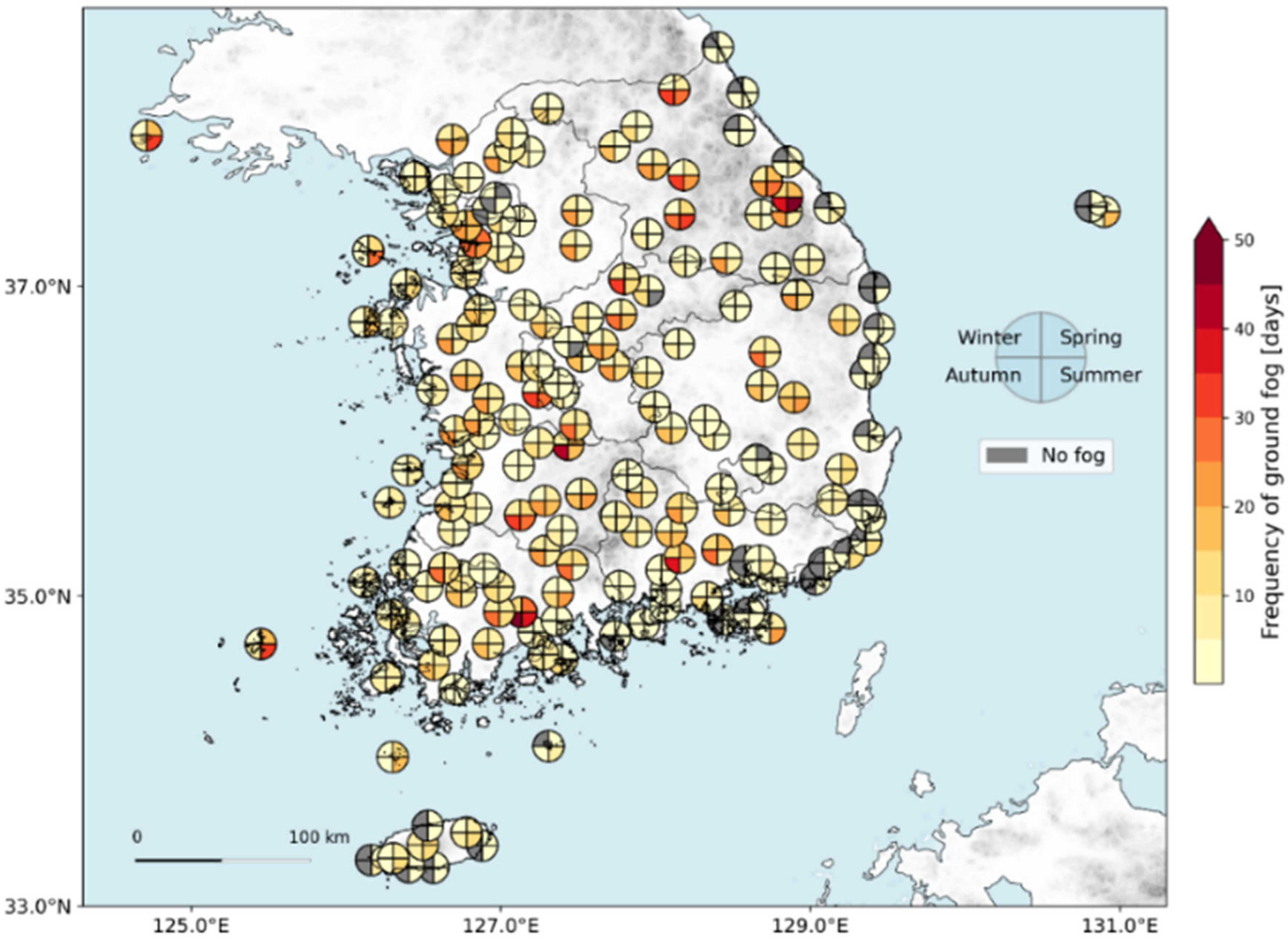
Remotesensing 17 02596 g002
Figure 3. The average annual number of fog occurrence days by season during 2021–2023 at 176 visibility meter stations. The quartered circular markers represent the seasonal fog frequency at each observation site. Each quadrant corresponds to a specific season in a clockwise order, starting from the top right corner: spring, summer, autumn, and winter.
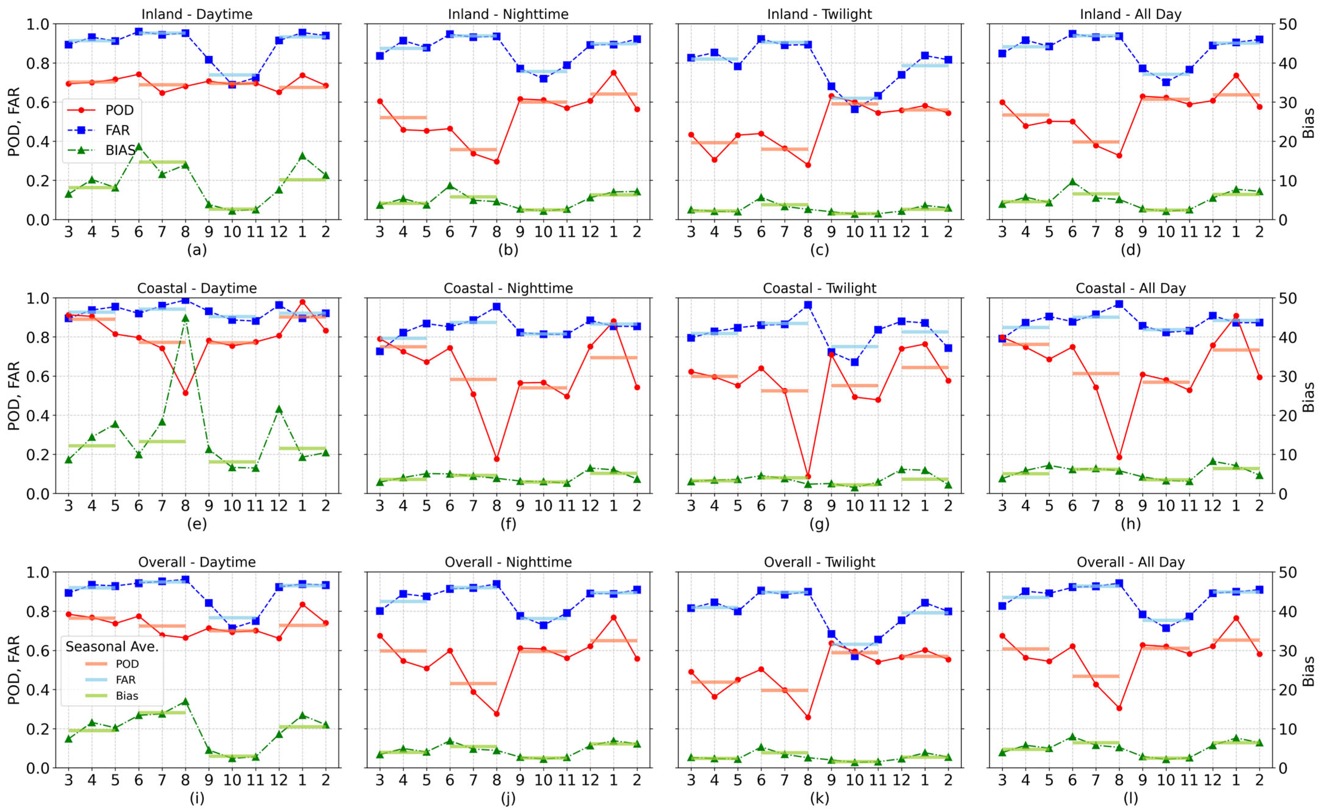
Remotesensing 17 02596 g003
Figure 4. Monthly and seasonal average detection performance (POD, FAR, and bias) of the GK2A_FDA over three years (2021–2023), categorized by time (daytime, nighttime, twilight) and geographic region (inland, coastal, overall). (a) Inland—Daytime, (b) Inland—Nighttime, (c) Inland—Twilight, (d) Inland—All Day, (e) Coastal—Daytime, (f) Coastal—Nighttime, (g) Coastal—Twilight, (h) Coastal—All Day, (i) Overall—Daytime, (j) Overall—Nighttime, (k) Overall—Twilight, (l) Overall—All Day.
Remotesensing 17 02596 g004
Figure 5. Monthly distribution of GK2A fog detection and ground fog occurrence frequency according to SZA at 4° intervals. The range of SZA changes with the month because SZA changes with the season. Daytime is defined as SZA < 80°, twilight as 80° ≤ SZA < 88°, and nighttime as SZA ≥ 88°. The data represent the annual frequency at 10 min intervals from 2021 to 2023. Missing bias values in low SZA bins indicate either no ground fog observations or values exceeding the axis range.
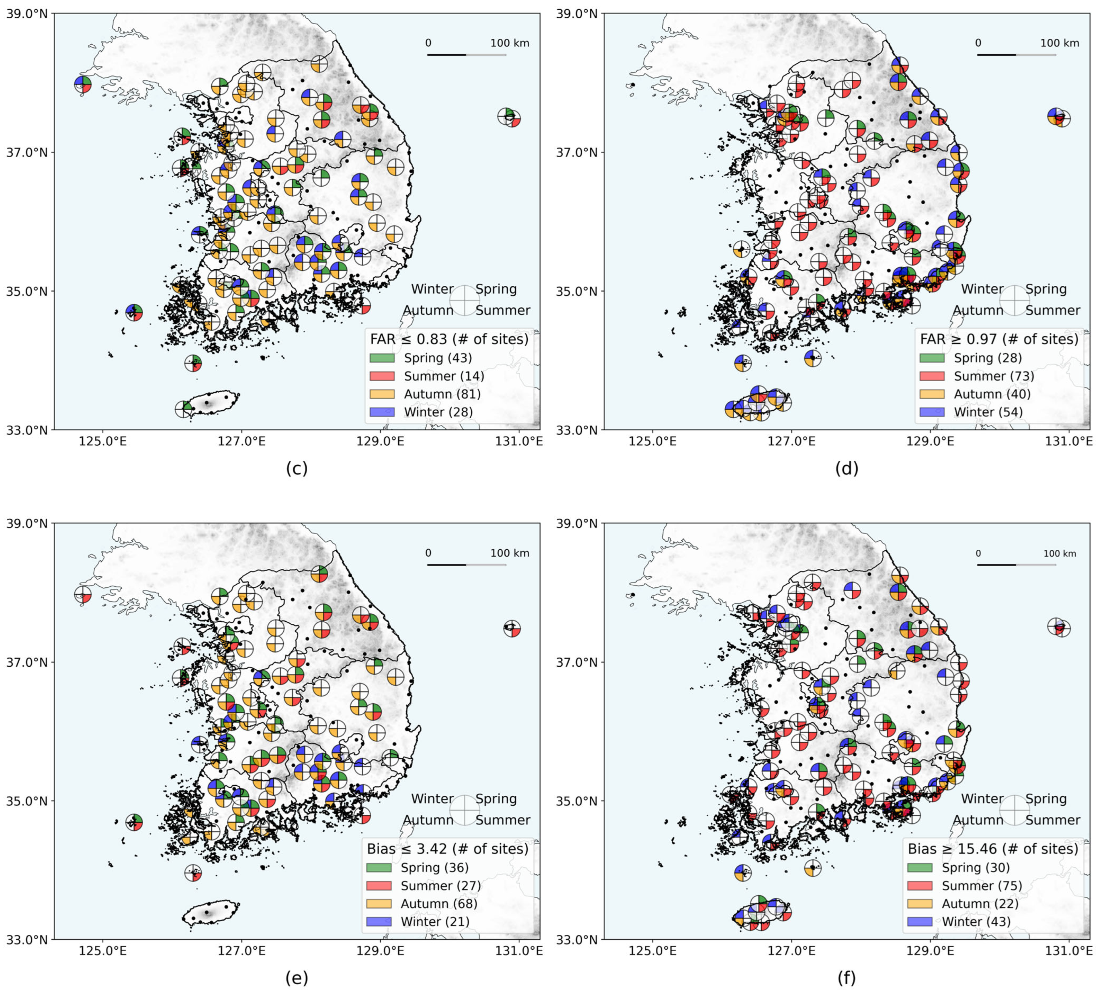
Remotesensing 17 02596 g005
Figure 6. Spatial distribution of visibility meter stations classified by the top and bottom 25% of seasonal frequency for GK2A fog detection performance: (a) POD ≥ 0.78 (top 25%), (b) POD ≤ 0.43 (bottom 25%), (c) FAR ≤ 0.83 (top 25%), (d) FAR ≥ 0.97 (bottom 25%), (e) bias ≤ 3.42 (top 25%), (f) bias ≥ 15.46 (bottom 25%). Quartered circular markers are displayed only at locations where the corresponding POD, FAR, or Bias values meet the specified thresholds.
Remotesensing 17 02596 g006aRemotesensing 17 02596 g006b
Figure 7. A time series analysis of the formation, development, and dissipation processes of radiation fog at Suwon located in the south-central region of Gyeonggi Province, South Korea, using (a) GK2A fog detection imagery, (b) fog detection result and ground visibility data, (c) GK2A cloud top height and ceilometer observations, and (d) ASOS meteorological data (period: 15:00 LST on 28 September to 15:00 on 29 September 2022).
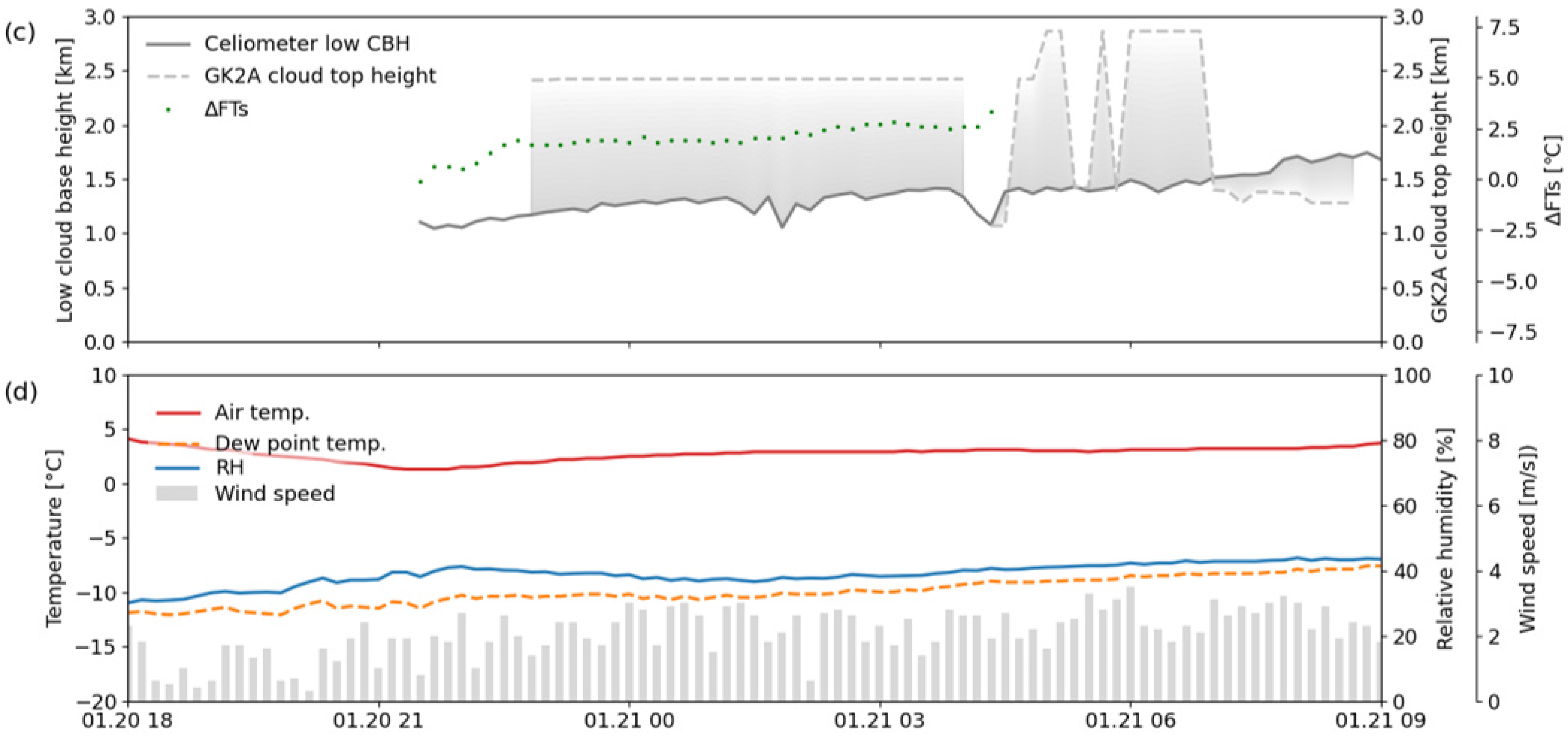
Remotesensing 17 02596 g007
Figure 8. A time series analysis of low stratus cases at Seoul using (a) GK2A fog detection imagery, (b) fog detection result and ground visibility data, (c) GK2A cloud-top height and ceilometer observations, and (d) ASOS meteorological data (period: 18:00 LST on 20 January 2021 to 09:00 LST on 21 January 2021).
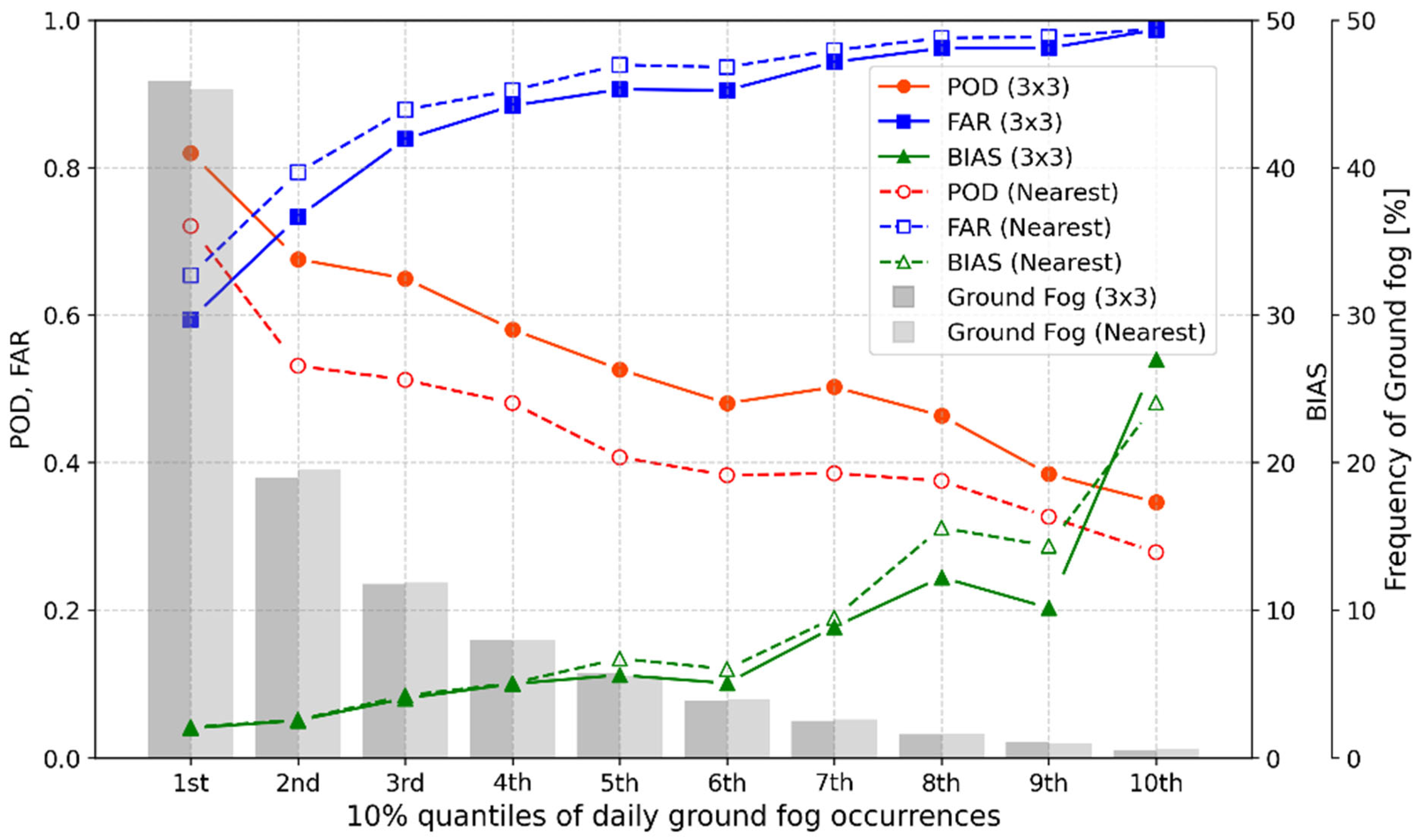
Remotesensing 17 02596 g008aRemotesensing 17 02596 g008b
Figure 9. The distribution of GK2A_FDA POD, FAR, and bias based on the 10% quantiles of daily ground fog occurrences from 2021 to 2023. The dashed and solid lines indicate that validation was performed by the nearest pixel and 3 × 3 neighborhood pixel methods, respectively.
Remotesensing 17 02596 g009
Figure 10. Monthly fog occurrence frequency detected by the visibility meter and GK2A_FDA (10 min interval) (2021–2023): (a) inland area, (b) coastal area.
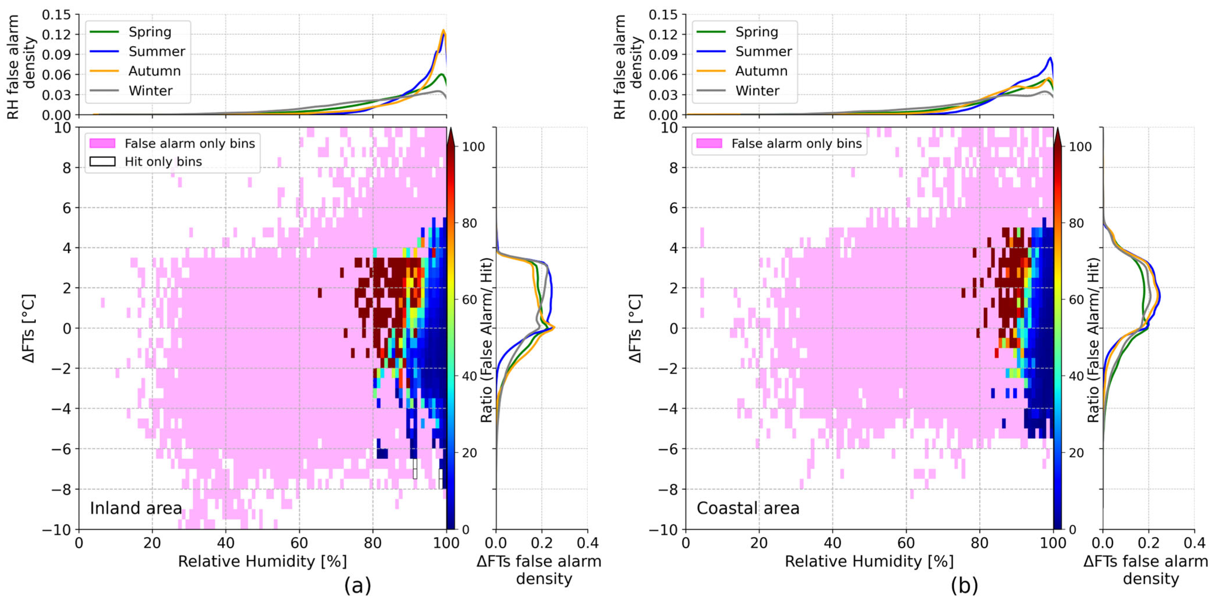
Remotesensing 17 02596 g010
Figure 11. Ratio distribution of false alarm counts to hit counts according to relative humidity and ΔFTs over (a) inland area and (b) coastal area, along with the frequency distribution of relative humidity (top) and ΔFTs (right) for each bin. The pink-shaded bins highlight zones of false alarm occurrences without corresponding hits in the GK2A fog detection.
Remotesensing 17 02596 g011
Figure 12. Ratio distribution of false alarm counts to hit counts according to relative humidity and SZA over (a) inland area and (b) coastal area, along with the frequency distribution of GK2A false detections by SZA bin (left).
Remotesensing 17 02596 g012
Table 1. Data used in the evaluation of the GK2A fog detection algorithm.
DataVariables [Unit]Spatial ResolutionTemporal ResolutionRemarks
GK2A FogFog, cloud, clear, etc.2 km10 min
Land sea maskLand, sea, coast2 km-
Visibility MeterVisibility [m]-1 min
ASOS/AWSRelative humidity [%],
temperature [°C],
wind speed [m s−1]
-1 minCase study
CeilometerLow cloud base height [m]10 m *10 minCase study
GK2A Cloud ProductCloud top height [m]2 km10 minCase study
* Vertical resolution.
Table 2. Summary of GK2A fog detection product.
NumberGK2A Fog ProductRemarks
1Clear sky-
2Middle/high cloud-
3UnknownPartially satisfy the fog criteria
4Probably fog -
5Fog-
6Snow-
7Desert or semi-desertPrefixed by land use
Table 3. 2 × 2 contingency table for the evaluation of the GK2A_FDA.
Ground Observation Fog (Visibility Meters)
Fog Non-Fog
GK2A
Fog
The nearest pixelFogHits (H) False alarms (F)
Non-fogMisses (M) Correct negative (C)
3 × 3 Neighborhood Pixel≥1Hits (H)≥5False alarms (F)
=0Misses (M)<5Correct negative (C)
Table 4. Proportion of quality flags in GK2A fog detection product at visibility meter stations, 2021–2023 (Flag 0: nominal, Flags 1–13: some channel data or previous time data missing, Flag 14: snow-contaminated, Flag 15: cloud-contaminated). The total scene count is 156,369.
Flag01~131415
Proportion [%]52.900.023.7343.34
Table 5. Overall performance of the GK2A fog detection algorithm by year (2021, 2022, 2023) and validation method (nearest pixel, 3 × 3 neighborhood pixel).
GK2A FogYearPODFARBias
The nearest pixel 20210.580.843.61
20220.590.885.13
20230.590.864.14
Ave.0.590.864.25
3 × 3 neighborhood pixel20210.690.773.04
20220.710.854.61
20230.700.813.70
Ave.0.700.813.73
Table 6. Summary of GK2A fog detection performance by region and time. Overall represents the combined statistics for inland and coastal regions.
PeriodInlandCoastalOverall
PODFARBiasPODFARBiasPODFARBias
Day0.690.896.120.830.9311.930.720.907.34
Night0.550.863.860.640.843.990.570.853.89
Twilight0.510.772.210.570.833.330.520.782.36
All day0.570.864.000.670.875.260.590.864.25
Table 7. Summary of GK2A fog detection performance by season.
SeasonPODFARBias
Spring0.610.874.72
Summer0.470.936.44
Autumn0.610.752.48
Winter0.650.906.43
Table 8. GK2A_FDA performance by the nearest pixel for individual scenes during the radiation fog event (03:00–09:00 LST on 29 September 2022, in Figure 7a).
Date (LST)PODFARBias
29 September 2022, 03:000.940.361.46
29 September 2022, 06:000.970.361.51
29 September 2022, 09:000.820.662.41
Disclaimer/Publisher’s Note: The statements, opinions and data contained in all publications are solely those of the individual author(s) and contributor(s) and not of MDPI and/or the editor(s). MDPI and/or the editor(s) disclaim responsibility for any injury to people or property resulting from any ideas, methods, instructions or products referred to in the content.

