Across-Beam Signal Integration Approach with Ubiquitous Digital Array Radar for High-Speed Target Detection

Abstract

Ubiquitous digital array radar (UDAR) extends the integration time of moving targets by deploying a wide transmitting beam and multiple narrow receiving beams to cover the entire observed airspace. By exchanging time for energy, it effectively improves the detection ability for weak targets. Nevertheless, target motion introduces severe across-range unit (ARU), across-Doppler unit (ADU), and across-beam unit (ABU) effects, dispersing target energy across the range–Doppler-beam space. This paper proposes a beam domain angle rotation compensation and keystone-matched filtering (BARC-KTMF) algorithm to address the “three-crossing” challenge. This algorithm first corrects ABU by rotating beam–domain coordinates to align scattered energy into the final beam unit, reshaping the signal distribution pattern. Then, the KTMF method is utilized to focus target energy in the time-frequency domain. Furthermore, a special spatial windowing technique is developed to improve computational efficiency through parallel block processing. Simulation results show that the proposed approach achieves an excellent signal-to-noise ratio (SNR) gain over the typical single-beam and multi-beam long-time coherent integration (LTCI) methods under low SNR conditions. Additionally, the presented algorithm also has the capability of coarse estimation for the target incident angle. This work extends the LTCI technique to the beam domain, offering a robust framework for high-speed weak target detection.

1. Introduction

With the continuous advancement in military science and technology, numerous high-speed targets have emerged in the field of radar detection. These targets typically exhibit characteristics such as hypersonic speed, high maneuverability, and weak reflected echoes, leading to the fact that the target energy is often insufficient to directly exceed the desired detection threshold [1,2,3,4].

Extending the observation time represents an efficacious approach to augment the signal-to-noise ratio (SNR) of the target output [5]. For conventional beam scanning radar, the beam dwell time in each direction is limited, which restricts the number of echoes available for coherent integration (CI) [6]. To further increase the detection probability, only the track information of multiple scanning periods can be utilized using non-coherent integration (NCI) [7,8]. However, as the amplitude information is exploited while the phase relationship among the signal pulses is overlooked, the accumulation effect of NCI processing remains relatively restricted. In contrast, the ubiquitous digital array radar (UDAR) can utilize multiple digital beamforming (DBF) technology to simultaneously form multiple resident narrow beams [9,10], enabling “staring” observation of the target space at the receiver. Consequently, the CI duration for UDAR is primarily determined by system hardware performance and target motion characteristics, rather than beam scanning time. This allows for a significant extension of CI time, achieving higher fusion accumulation gains and superior detection capabilities.

In fact, for conventional targets with a large Radar Cross Section (RCS), the target echo energy collected by the radar during the illumination of a single beam is sufficient to exceed the detection threshold. Therefore, conventional targets generally do not require consideration of the across-beam accumulation issue. However, high-speed targets such as anti-ship missiles over the sea and near-space cruise vehicles are highly likely to traverse multiple observation beams during prolonged observation, resulting in the effective accumulation time of the target within a single beam being strictly limited. Thus, target energy accumulation and detection processing for such targets in UDAR face critical challenges, including:

(1)

Intra-beam target motion compensation: In practical scenarios, when a moving target crosses multiple beams during coherent integration, its entry and exit times from each beam cannot be pre-determined, as the target may enter the radar coverage area unexpectedly and depart after an indefinite period. Meanwhile, target motion induces across-range unit (ARU) and across-Doppler unit (ADU) effects, rendering traditional moving target detection (MTD) methods highly ineffective and causing severe performance degradation in target focusing.

(2)

Inter-beam signal fusion processing: Due to the tangential time-varying characteristics between target motion and different dwell beams, signal phases and envelope positions vary across beams. This necessitates addressing radar echo signal accumulation challenges across inter-beam domains.

Therefore, studying the LTCI method under the “three-crossing” situation is of crucial importance for improving the detection ability of high-speed targets.

Recently, numerous excellent LTCI research papers have been proposed on high-speed target detection. In order to address the ARU effect, these investigations can be mainly divided into the nonsearching-based approaches and the searching-based approaches. The former typical methods usually indicate the nonlinear algorithm, including the scaled inverse Fourier transform (SCIFT) [11], frequency–domain deramp-processing (FDDKT) [12], adjacent cross correlation function (ACCF) [13], and sequence-reversing transform (SRT) [14,15,16]. The core idea of these algorithms is to use the correlation function to eliminate the order of motion parameters. When achieving the decoupling of motion parameters from the time domain, the complexity of signal components is also reduced. Although the nonsearching-based approaches are computationally efficient, they sacrifice target accumulation performance under low SNR scenarios, and nonlinear processing would make the multi-target cross terms affect the detection performance. For the latter, the typical searching-based approaches contain keystone transform (KT) [17], axis-rotation transform (ART) [18,19,20,21], and Radon Fourier transform (RFT) [22,23]. The KT [24] corrects the ARU effect via searching the Doppler fold factor and rescaling the slow-time dimension. ART carries out axis rotation to match the optimal rotated angle to achieve target energy accumulation. In addition, RFT adopts Radon’s idea to accumulate energy along the target trajectories by simultaneously searching for the target’s motion parameters. In particular, these algorithms feature simple yet effective ideas and can obtain great SNR gain without appreciable energy loss. Nevertheless, it is further noted that highly accurate parameter estimation results often require a refined parameter search process, which implies that the above algorithms cause a huge computational burden. Sometimes, if there is certain prior information for guidance, the computational complexity can be appropriately reduced.

In terms of settling ADU and ARU effects, current representative algorithms can be divided into two categories: Joint processing (JP) mode and step processing (SP) mode. JP methods define that the envelop and phase compensation functions are constructed to simultaneously remove ARU and ADU effects. For example, the generalized Radon-Fourier transform (GRFT) [25] and RFT-based methods [26,27] are highly representative algorithms. The key work of these algorithms is that the signal envelopes from time domain echoes are extracted by multidimensional joint searching all possible target motion states and constructing the specific Doppler filters to compensate for the ADU. Then, target signals could be focused on as the peaks in the output parameter domain. However, if the parameter searching space is unavoidably large for high-order target motions, these algorithms would inevitably encounter high computational complexity. In spite of the excellent CI gain that can be obtained in these methods, the ergodic search operation in Radon-based methods will inevitably introduce an unbearable computational burden. Additionally, blind speed sidelobe (BSSL) may lead to the integrated peak of the weak target being masked by sidelobes of the strong one, causing severe miss alarms and false alarms [28]. The main idea of SP algorithms means that they eliminate ARU at first and then remove ADU effect to achieve the accumulation of target energy, which can be further subdivided into three categories, i.e., AR-based methods, KT-based methods, and correlation-based methods. AR-based methods contain the modified AR and Lv’s distribution (MAR-LVD) [29], improved AR and discrete chirp-Fourier transform (IAR-DCFT) [30], and IAR and fractional Fourier transform (IAR-FRFT) [31]. Typical KT-based methods contain second-order KT [32], KT and matched filtering process (KT-MFP) [33,34,35], and other modified KT-based methods [36,37]. In these KT-based methods, a certain order of RM can be first removed by KT or modified KT technique, resulting in computation efficiency improvement, while they may not deal with high-order maneuvering motions and high-speed targets with Doppler ambiguity. To alleviate the computation complexity, the correlation-based methods generally design a particular nonlinear kernel function to reduce the phase order of the radar returns and effectively alleviate the influence of the ARU and ADU, leading to a rapid detection strategy. Typical correlation-based methods include the frequency reversal and LVD (FR-LVD) [38], improved time reversal transform and modified Radon Fourier transform (ITRT-MRFT) [39], and three-dimensional scaled transform (TDST) [40,41]. Unfortunately, nonlinear operations may lead to unexpected performance losses and generate cross terms when handling multi-target detection.

All the mentioned LTCI methods mainly focus on the parameter estimation and signal accumulation in the radial direction, but they neglect the across-beam unit (ABU) effects caused by tangential target motion. In fact, there are relatively few studies for the ABU correction. Reference [42] proposed the time-shared multi-beam (TSMB) and space-shared multi-beam (SSMB) based on digital array radar, but it only considered the pointing phase difference between different beams and did not note the existence of ARU and ADU; hence, it has certain limitations. To address problems that occur when the moving target enters and leaves the beam is unknown, the short-time generalized Radon Fourier transform (STGRFT) [43] and window Radon Fractional Fourier transform (WRFRT) [44] are proposed to detect and estimate the target’s time parameters, respectively. However, the integration within the inter-beam is not considered in [43,44]. Moreover, the multiple-beams joint integration algorithm based on the spatial projection method (i.e., MBPCF-MSWPD) is developed in [45], which applies the multi-beam phase compensation function to correct the difference between different beams, and a multi-scale sliding windowed phase difference is utilized to estimate the unknown time information. After that, it realizes well-focused output within the inter-beam. Nevertheless, this NCI method in [45] is only suitable for full beams processing; the target prior location needs to be provided, and a multidimensional search operation requires a huge computational complexity.

In this paper, an across-beam target energy accumulation approach for high-speed target detection with the UDAR system is presented. The core idea is to perform signal fusion processing across adjacent beams, which effectively enhances the detection capability for high-speed targets by coherently aggregating energy dispersed across beam boundaries. Furthermore, the study’s significance lies in that it extends the degree of freedom in signal processing of LTCI methods to beam–space integration based on the multi-beam forming. In detail, the main innovation points of our work are summarized as follows.

• The across-beam three-dimensional (3D) signal model for a high-speed target with UDAR is established first, illustrating the phase and envelope properties between intra-beam and inter-beam. On this basis, the beam segmentation characteristics of the across-beam received signals are described. Then, the detailed constraint conditions for the “three-crossing” effects, including the ARU, ADU, ABU, and the coherent signal constraint, are analyzed through mathematical expressions.
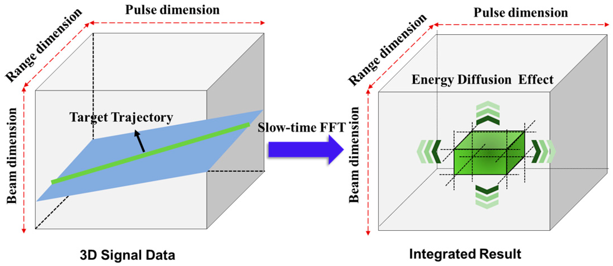
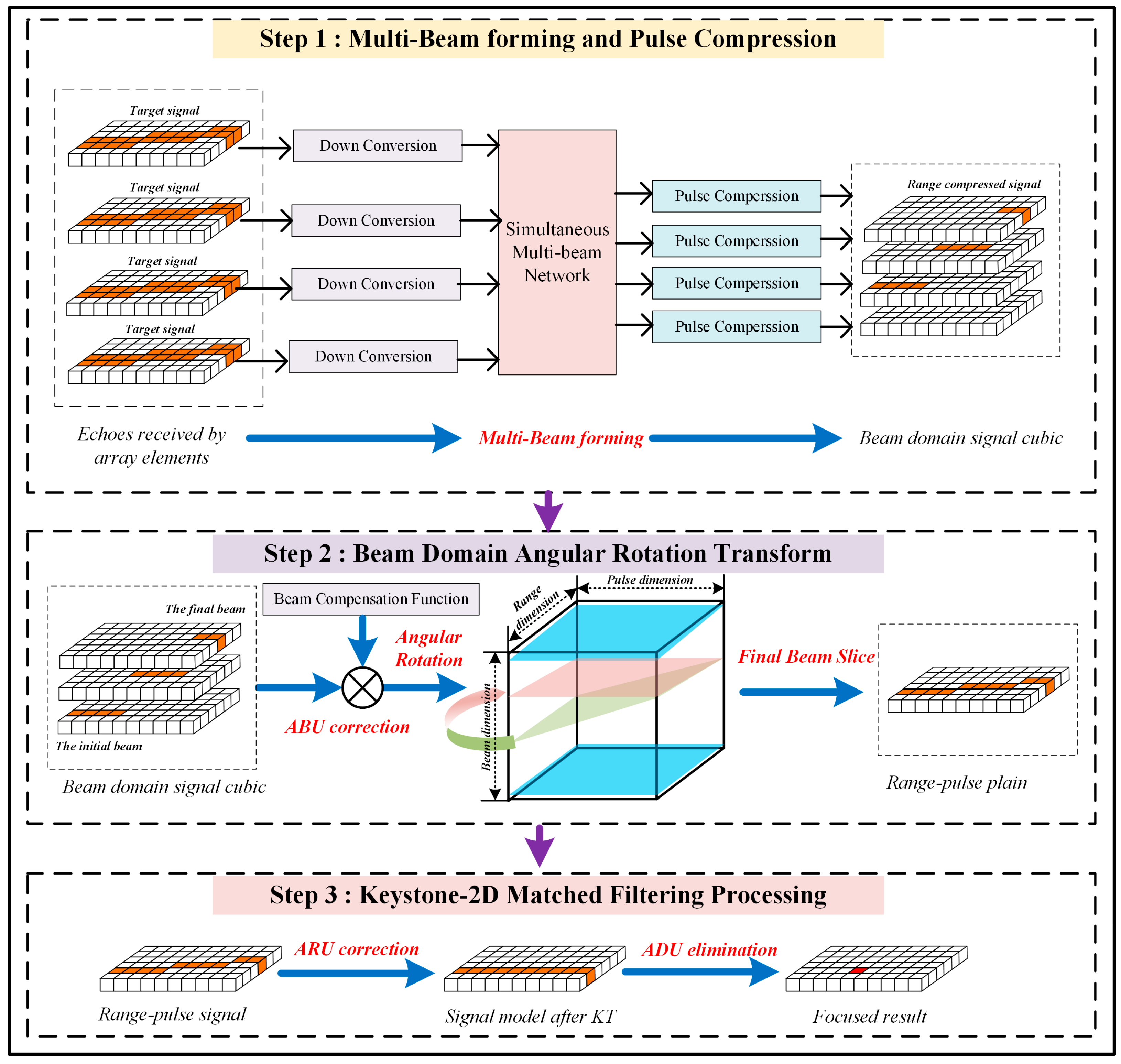
• Owing to the tangential angular velocity of high-speed target coupling with slow time, the target energy distribution appears as an inclined stepped platform in the 3D signal model. Then, inspired by AR-based algorithms [18,19,20,21], we propose the beam–domain rotation compensation (BARC) approach to correct the ABU effect. After dwell beam compensation and spatial angle rotation, the target energy of the beam domain can be assigned to the same beam unit. Afterwards, the keystone-matched filter method (KTMF) can be applied to remove ARU and ADU effects. It (i.e., BARC-KTMF) realizes well-focused output on the final beam, and the improved detection performance can be obtained.
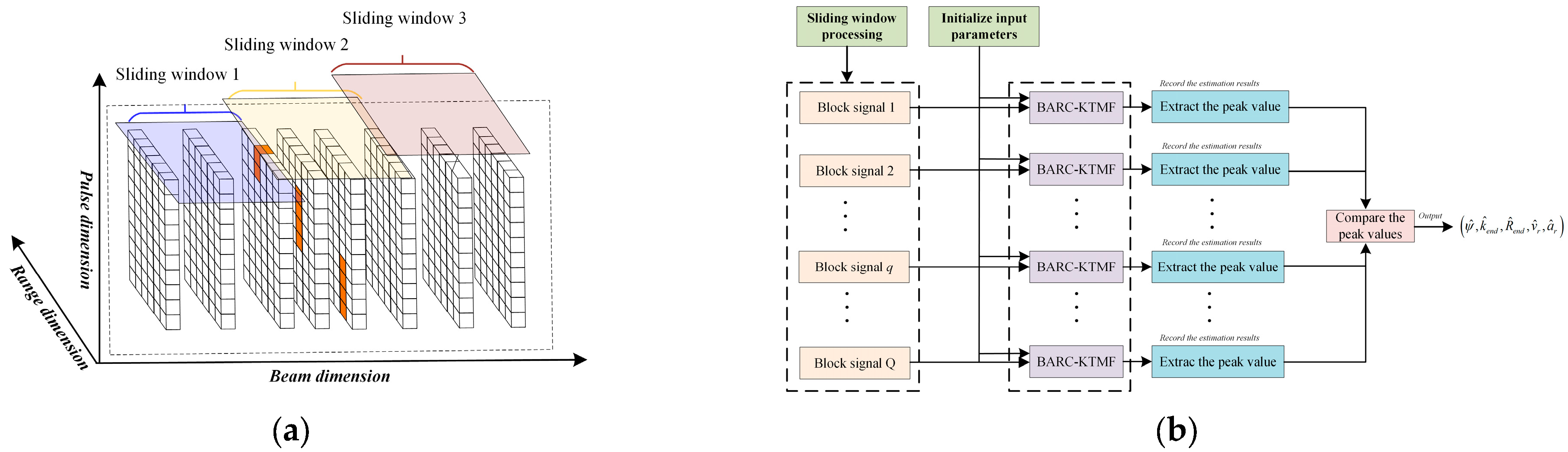
• Considering the huge computational complexity of full-beam processing, under the coherence constraint conditions, a kind of spatial windowing processing approach is developed to improve the across-beam accumulation efficiency, and the detailed execution procedures are also provided.
• In addition, to verify the validity of this algorithm, numerical simulations for different scenarios are provided to examine the performance of the proposed method, i.e., integration performance for single target, integration performance for multiple targets, detection ability comparison with some existing methods. Experiment results indicate that the accumulation and detection performance of the proposed method are significantly improved.

The remainder of this paper is organized as follows. The system description and model analysis for the high-speed target with UDAR are presented in Section 2. Then, the detailed across-beam coherent integration method is formulated in Section 3. Section 4 demonstrates the algorithm performance analysis discussions for the proposed approach. Next, Section 5 gives simulation and experiment results to verify the effectiveness and reliability of the proposed algorithm. Moreover, some challenging works are summarized in Section 6. Finally, the conclusions of this paper are drawn in Section 7.

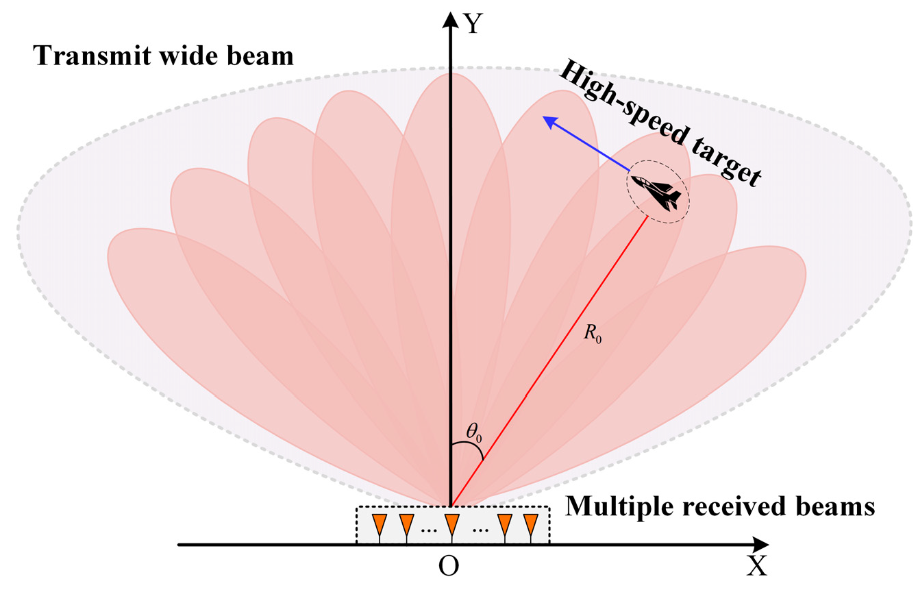
2. System Description and Model Analysis

In this section, we first provide the across-beam 3D signal model with the UDAR to introduce “three-crossing” effects. Furthermore, the beam segmentation characteristics of the received signals are presented to depict the target energy distribution within the intra-beam. Finally, the constraint conditions for “three-crossing” effects are also given, which contain ARU, ADU, and ABU. And then the coherent signal constraint is also considered.

2.1. The Across-Beam 3D Signal Model

As shown in Figure 1, we consider a UDAR system composed of a uniform linear array with L array elements in the 2D plane of distance and azimuth. As for this radar system, it can effectively cover the observation area by transmitting a wide beam and using multiple received beams. At the emitter end, the narrowband linear frequency modulated (LFM) pulse waveform is used as the transmitted signal, which can be formulated as follows:

$$s\left(t\right)=\sqrt{E}x\left(t\right)\exp \left(j2\pi f_{c}t\right)$$

(1)

where $E$ indicates the emitted power, $t$ represents the time variable, $f_c$ is the radar carrier wave frequency, and $x\left(t\right)$ is the complex envelope of the transmitted baseband signal, which is denoted by the following:

$$x\left(t\right)=\mathrm{rect}\left({\displaystyle \frac{t}{T_p}}\right)\exp \left(j\pi \mu t^2\right)$$

(2)

where $\mu =B/T_p$ denotes the linear frequency modulation rate of the LFM waveform with signal bandwidth B and pulse duration $T_p$. $\mathrm{rect}\left(t/T_p\right)=\left\{\begin{array}{cc}1,\hfill & \left|t\right|\le T_p/2\hfill \\ 0,\hfill & \left|t\right|>T_P/2\hfill \end{array}\right.$ represents the rectangular window function.

For convenience, assume that there is one high-speed target rapidly traversing the beams within the radar detection range, whose fluctuation distribution satisfies the Swerling I model. At the receiver end, the group of reflected pulse train signals propagates through free space to the array elements. Therefore, after the down conversion operation, the received echo of the l-th element can be expressed as follows:

$$\begin{array}{cc}{\mathrm{s}}_r\left(l;t_n,t_m\right)& ={\beta }_1\stackrel{\mathrm{signal} \mathrm{term}}{\overbrace{\mathrm{rect}\left({\displaystyle \frac{t_n-\tau \left(t_m\right)}{T_p}}\right)\exp \left[j\pi \mu {\left(t_n-\tau \left(t_m\right)\right)}^2\right]\exp \left(-j2\pi f_c\tau \left(t_m\right)\right)}}\\ & \times \underset{\mathrm{spatial} \mathrm{steering} \mathrm{vector}}{\underbrace{\exp \left[-j{\displaystyle \frac{2\pi f_c}{c}}\left(l-1\right)d\sin \theta \left(t_m\right)\right]}}\end{array}$$

(3)

where ${\beta }_1$ is the amplitude of the received echo, $t_n$ denotes the fast-time variable, and $\tau \left(t_m\right)=2R\left(t_m\right)/c$ represents the time delay term with respect to the slow-time $t_m$. $R\left(t_m\right)$ denotes the instantaneous slant distance between the target and the radar under the “go-step-go” model. Furthermore, the relationship between target and radar can be jointly characterized in the tangential and radial directions as follows:

$$\left\{\begin{array}{c}R\left(t_m\right)=R_0+v_r{t}_m+{\displaystyle \frac{1}{2}}{a}_r{t}_m^2\\ \theta \left(t_m\right)={\theta }_0+\omega t_m\end{array}\right.$$

(4)

where $R_0$ presents the initial slant distance, $v_r$ represents the radial velocity, $a_r$ is the radial acceleration, ${\theta }_0$ denotes the initial angle between the initial slant distance and the Y axis direction, and $\omega$ is the angular velocity of the target along the tangential direction.

For the UDAR system, suppose that there are $K$ dwell beams to cover the observation space. Then, the simultaneous multi-beam received weight vectorizer ${\Omega }_{\mathrm{w}}$ can be expressed as

$$\begin{array}{c}{\Omega }_{\mathrm{w}} =[a\left({\theta }_1\right),a\left({\theta }_2\right),\cdots ,a\left({\theta }_K\right)]\\ =\left[\begin{array}{cccc}1& 1& \cdots & 1\\ \exp \left(j{\displaystyle \frac{2\pi }{\lambda }}d\sin {\theta }_1\right)& \exp \left(j{\displaystyle \frac{2\pi }{\lambda }}d\sin {\theta }_2\right)& \cdots & \exp \left(j{\displaystyle \frac{2\pi }{\lambda }}d\sin {\theta }_K\right)\\ ⋮& ⋮& \ddots & ⋮\\ \exp \left[j{\displaystyle \frac{2\pi }{\lambda }}\left(l-1\right)d\sin {\theta }_1\right]& \exp \left[j{\displaystyle \frac{2\pi }{\lambda }}\left(l-1\right)d\sin {\theta }_2\right]& \cdots & \exp \left[j{\displaystyle \frac{2\pi }{\lambda }}\left(l-1\right)d\sin {\theta }_K\right]\end{array}\right]\in {ℂ}_{L\times K}\end{array}$$

(5)

where ${\theta }_i$ is the beam pointing angle with respect to the i-th received beam, $a\left({\theta }_i\right)$ denoted the weight vector of the dwell beam associated with ${\theta }_i$.

Through the multi-beamforming to realize spatial domain filtering processing, the beam domain echo data $s_{\mathrm{Beam}}$ can be obtained by the following:

$$s_{\mathrm{DBF}}\left({\theta }_k;t_n,t_m\right)={\Omega }_w{\mathrm{s}}_r\left(l;t_n,t_m\right)$$

(6)

Applying Equation (5) to Equation (3), Equation (6) could be rewritten as follows:

$$\begin{array}{cc}{\mathrm{s}}_{\mathrm{DBF}}\left({\theta }_k;t_n,t_m\right)& ={\beta }_2\mathrm{rect}\left({\displaystyle \frac{t-\tau \left(t_m\right)}{T_p}}\right)\exp \left[j\pi \mu {\left(t-\tau \left(t_m\right)\right)}^2\right]\exp \left(-j2\pi f_c\tau \left(t_m\right)\right)\hfill \\ & \times \mathrm{sinc}\left[-{\displaystyle \frac{\pi Ld\tilde{\eta }}{4\lambda }}\left({\theta }_k-{\theta }_0-\omega t_m\right)\right]\exp \left[-j{\displaystyle \frac{\pi d\left(L-1\right)}{\lambda }}\sin {\theta }_k\right]\hfill \end{array}$$

(7)

where ${\beta }_2=L\beta$ is the enhanced amplitude after the DBF operation, and $\tilde{\eta }$ is the auxiliary variable associated with ${\theta }_k$. The detailed derivation of Equation (7) is given in Reference [46].

Substituting Equation (4) into Equation (7) and performing a matched filter operation along the $t_n$ dimension, such that the signal after pulse compression (PC) is given as follows:

$$\begin{array}{cc}{s}_{\mathrm{pc}}\left({\theta }_k;t_n,t_m\right)& =A_{1m}\mathrm{sinc}\left\{B\left[t_n-{\displaystyle \frac{2\left(R_0+v_r{t}_m+0.5a_r{t}_m^2\right)}{c}}\right]\right\}\exp \left[-j{\displaystyle \frac{4\pi }{\lambda }}\left(R_0+v_r{t}_m+{\displaystyle \frac{1}{2}}{a}_r{t}_m^2\right)\right]\hfill \\ & \times \mathrm{sinc}\left[-{\displaystyle \frac{\pi Ld\tilde{\eta }}{4\lambda }}\left({\theta }_k-{\theta }_0-\omega t_m\right)\right]\exp \left[-j{\displaystyle \frac{\pi d\left(L-1\right)}{\lambda }}\sin {\theta }_k\right]\hfill \end{array}$$

(8)

where $A_{1m}={\beta }_2\sqrt{T_{p}B}$ is the signal amplitude after PC, and $\mathrm{sinc}\left[x\right]=\sin \left(\pi x\right)/(\pi x)$ represents the sinc function.

Next, we perform discretization processing on the signal (8). Let $t_n=2r/c$, where $r$ denotes the radial distance with respect to the fast-time $t_n$. Further, Equation (8) can be recast as

$$\begin{array}{cc}{s}_{\mathrm{beam}}\left(\theta ;r,t_m\right)& =A_{1m}\mathrm{sinc}\left\{{\displaystyle \frac{2B}{c}}\left[r-\left(R_0+v_r{t}_m+{\displaystyle \frac{1}{2}}{a}_r{t}_m^2\right)\right]\right\}\exp \left[-j{\displaystyle \frac{4\pi }{\lambda }}\left(R_0+v_r{t}_m+{\displaystyle \frac{1}{2}}{a}_r{t}_m^2\right)\right]\hfill \\ & \times \mathrm{sinc}\left[-{\displaystyle \frac{\pi Ld\tilde{\eta }}{4\lambda }}\left({\theta }_k-{\theta }_0-\omega t_m\right)\right]\exp \left[-j{\displaystyle \frac{\pi d\left(L-1\right)}{\lambda }}\sin {\theta }_k\right]\hfill \end{array}$$

(9)

Generally, the range sampling frequency is set as $f_s=2B$, and $\Delta r=c/2f_s$ denotes the range sampling unit. For simplicity, the beam sampling interval is defined as 3 dB beam width $\Delta \theta$. Therefore, the discrete beam domain echo signal can be expressed as

$$\begin{array}{cc}{s}_{\mathrm{beam}}\left(n,m,k\right)& =A_{1m}\stackrel{\mathrm{Part} \mathrm{A}}{\overbrace{\mathrm{sinc}\left\{{\displaystyle \frac{1}{2}}\left[n-n_0-{\displaystyle \frac{v_{r}m{T}_r+0.5a_r{\left(m{T}_r\right)}^2}{\Delta r}}\right]\right\}}}\stackrel{\mathrm{Part} \mathrm{B}}{\overbrace{\exp \left\{-j{\displaystyle \frac{4\pi }{\lambda }}\left[R_0+v_{r}m{T}_r+{\displaystyle \frac{1}{2}}{a}_r{\left(m{T}_r\right)}^2\right]\right\}}}\hfill \\ & \times \underset{\mathrm{Part} \mathrm{C}}{\underbrace{\mathrm{sinc}\left[-{\displaystyle \frac{\pi Ld\tilde{\eta }\Delta \theta }{4\lambda }}\left(k-k_0-{\displaystyle \frac{\omega m{T}_r}{\Delta \theta }}\right)\right]}}\underset{\mathrm{Part} \mathrm{D}}{\underbrace{\exp \left[-j{\displaystyle \frac{\pi d\left(L-1\right)}{\lambda }}\sin \left({\theta }_k\right)\right]}}\hfill \end{array}$$

(10)

where k denotes the index of the received beam, and $k_0=\mathrm{round}\left[\left({\theta }_0-{\theta }_1\right)/\Delta \theta \right]$ indicates the beam unit index related to the initial angle ${\theta }_0$. $n=\mathrm{round}\left[r/\Delta r\right]$ is the index of range variable, $n_0=\mathrm{round}\left[R_0/\Delta r\right]$ is the range unit of the initial radial distance, and m represents the m-th received pulse. And $\mathrm{round}\left[·\right]$ denotes the roundup operation. The beam domain echoes could be divided into four parts.

• Part A expresses the signal envelope of range dimension and pulse dimension, where the radial velocity $v_r$ and radial acceleration $a_r$ are coupled with variable m.
• Part B is a phase term associated with the radial motion of the target.
• Part C is the envelope position term with respect to the azimuth angle, where the tangential angular velocity $\omega$ is also coupled with variable m, leading to the varying azimuth angle.
• Part D denotes the dwell beam phase term.

As can be seen from Equation (11), Part A and Part C indicate that the radial signal envelope would change with velocity and acceleration, and the changed azimuth angle results in the tangential signal position shifted along the beam dimension. Thus, ARU, ADU, and ABU effects will occur. Figure 2 illustrates the sketch map of the 3D signal model, where the target trajectory appears as an inclined diagonal line in space. Moreover, if the traditional MTD is used to achieve CI, the target energy will be diffused in the range Doppler-beam three dimensions, which leads to a decrease in integrated gain.

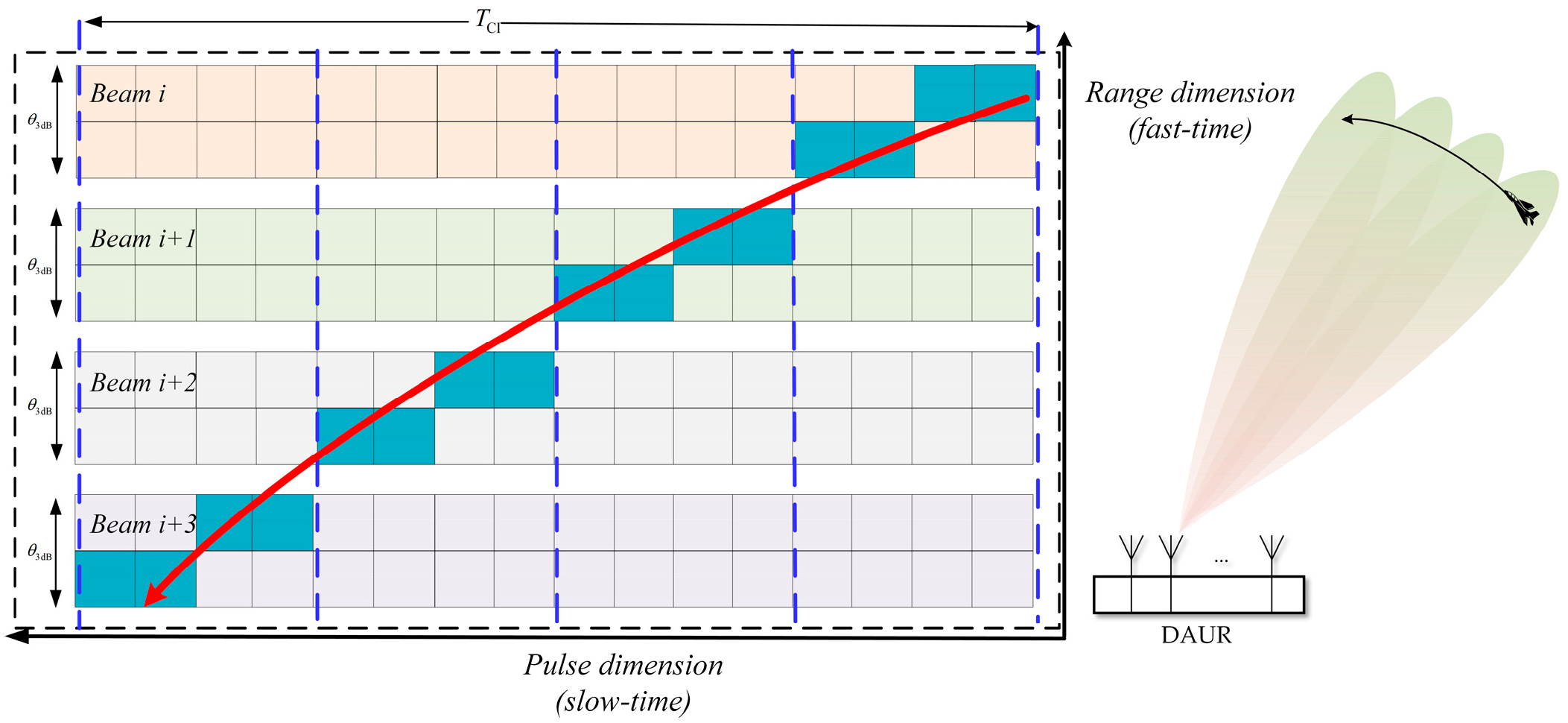
2.2. The Beam Segmentation Characteristics of the Aacross-Beam Received Signals

In this subsection, the beam segment characteristics within the intra-beam are briefly analyzed. To clarify the across-beam effect, this paper simplifies the target motion model and only considers the uniform tangential angular velocity. The complex tangential motion model will be further studied in the subsequent scientific research work. From Equation (10), Part C expresses the signal energy distribution along the beam dimension. There are three factors affecting the target’s beam domain echo envelope: the initial incident angle of the target, the target tangential angular velocity, and the beam width. Since the main energy of the sinc function is concentrated within the half-power width, the signal intensity outside of this part decreases significantly. This is similar to adding a sliding window function in the beam dimension. For the possible beams of a certain high-speed target, the time when the target flies into and out of these beams is actually unknown. Therefore, we assume that the target exists in the i-th receiving beam. If the azimuth modulation effect can be modeled as the window function, Equation (9) could be rewritten as follows:

$$\begin{array}{cc}{s}_{\mathrm{beam},\mathrm{i}}\left(t_n,t_m\right)& ={\tilde{\beta }}_2\mathrm{rect}\left[{\displaystyle \frac{t_m-0.5\left(T_{\mathrm{init},\mathrm{i}}+T_{\mathrm{end},,\mathrm{i}}\right)}{T_{\mathrm{init},\mathrm{i}}-T_{\mathrm{end},,\mathrm{i}}}}\right]\mathrm{sinc}\left\{B\left[t_n-{\displaystyle \frac{2\left(R_0+v_r{t}_m+0.5a_r{t}_m^2\right)}{c}}\right]\right\}\hfill \\ & \times \exp \left[-j{\displaystyle \frac{4\pi }{\lambda }}\left(R_0+v_r{t}_m+{\displaystyle \frac{1}{2}}{a}_r{t}_m^2\right)\right]\exp \left[-j{\displaystyle \frac{\pi d\left(L-1\right)}{\lambda }}\sin {\theta }_i\right]\hfill \end{array}$$

(11)

where $T_{\mathrm{init},\mathrm{i}}$ represents the input time when the target flies into the i-th beam, and $T_{\mathrm{end},,\mathrm{i}}$ represents the output time when the target flies out of the i-th beam. In fact, $\Delta T_i=T_{\mathrm{end},,\mathrm{i}}-T_{\mathrm{init},\mathrm{i}}$ denotes the integration time within the i-th beam. Figure 3 shows the beam segmentation characteristics, where the target signals are scattered among adjacent beams. Therefore, the core idea of solving the ABU effect is to make full use of the different $\Delta T_i$ to enhance the weak target energy. Reference [45] utilizes the multi-scale sliding windowed phase difference method to estimate the unknown time information, and then the effective target signal can be extracted. However, this searching operation for each beam will bring about a huge computational burden. Thus, to overcome the above-mentioned difficulties in ABU correction, this paper proposes the beam domain angular rotation approach in Section 3.

2.3. The Constraint Conditions for the “Three-Crossing” Effects

In this subsection, we conduct a further analysis of “three-crossing” effects. And four kinds of constraint conditions are provided, including ABU, ARU, ADU, and the coherent signal constraint.

2.3.1. ABU Effect Analysis

From Equation (8), the azimuth angle corresponding to the target is varied with the slow-time variable m. During the long, coherent time, the azimuth angle maximum offset can be expressed as follows:

$$\Delta {\theta }_d=\left|\max \left(\theta \left(t_m\right)\right)-\min \left(\theta \left(t_m\right)\right)\right|$$

(12)

where $\Delta \theta \approx 102/L$ represents the angular resolution (i.e., the 3 dB beam width, ${\theta }_{3dB}$). Therefore, when the angle offset exceeds one angular resolution, the target energy will scatter into different beams. It means that the ABU effect occurs. Furthermore, the condition of ABU can be given by the following:

$$\omega T_{CI}>\Delta \theta$$

(13)

where $\omega =v_t/R_0$ is the tangential angular velocity related to the radial initial distance $R_0$ and tangential velocity $v_t$, $T_{Ci}=M{T}_r$ is the full observation time, and M denotes the received pulse numbers. Here, a simple example is given to analyze the ABU issues. We assume that a target moving at 300 m/s with a radial distance of 10 km can generate an angular velocity of approximately 0.03 rad/s; over a typical integration time around 5 s, this results in a tangential motion of about 8°, easily spanning four beams (assuming a 3 dB beamwidth of 2°). Such tangential motion directly causes the target signal to leak across adjacent beams.

2.3.2. ARU Effect Analysis

As can be seen from Equation (8), the distance offset from the changed range position of the target can be formulated as follows:

$$\Delta R\left(t_m\right)=\left|\max \left(R\left(t_m\right)\right)-\min \left(R\left(t_m\right)\right)\right|$$

(14)

where $\Delta r$ represents the range sampling unit.

Generally, the ARU effect could be divided into two conditions. The ARU effect resulting from the radial velocity is called the first-order range migration (FRM), which can be expressed as follows:

$$\Delta R_{FRM}\left(t_m\right)=\left|v_r{T}_{Ci}\right|>\Delta r$$

(15)

Then, the ARU effect resulting from the radial acceleration is also named the second-order range migration (SRM), and it can be given as follows:

$$\Delta R_{SRM}\left(t_m\right)=\left|0.5a_r{T}_{CI}^2\right|>\Delta r$$

(16)

Moreover, for the high-speed target, the range offset resulting from the radial acceleration exceeds one range sampling unit. In this case, the range curve effect cannot be neglected.

2.3.3. ADU Effect Analysis

When the Doppler frequency offset exceeds a Doppler resolution unit, the signal energy would spread into different Doppler frequency channels. That is why the traditional MTD is inactive for integrating the target signal. In terms of Equation (8), the Doppler frequency can be formulated as follows:

$$f_d\left(t_m\right)=-{\displaystyle \frac{2}{\lambda }}{\displaystyle \frac{dR\left(t_m\right)}{d{t}_m}}=-{\displaystyle \frac{2}{\lambda }}\left(v_r+a_r{t}_m\right)$$

(17)

Then, the ADU condition resulting from the Doppler frequency offset can be expressed as follows:

$$\begin{array}{cc}\Delta f_d\left(t_m\right)& =\left|\max \left(f_d\left(t_m\right)\right)-\min \left(f_d\left(t_m\right)\right)\right|\hfill \\ & =\left|-{\displaystyle \frac{2a_r{T}_{CI}}{\lambda }}\right|>{\Delta }_{f_d}\hfill \end{array}$$

(18)

where ${\Delta }_{f_d}=1/T_{Ci}$ represents the Doppler resolution. Thus, the AUD effect mainly depends on the target radial acceleration and the Doppler resolution unit.

2.3.4. The Coherent Signal Constraint

When the radar beam illuminates a target for an extended period, the target movement and position rotation would change in the illuminated part of the target, resulting in the “RCS scintillation”. And “RCS scintillation” will lead to a decrease in the correlation of the echo signals, affecting the CI performance. Inspired by Literature [47], Appendix A studies the influences of different change angles, different carrier frequencies, and target sizes on the correlation of signal echoes. Figure 4 indicates the simulation results. Figure 4a presents the curves of the correlation coefficient affected by the observation angle and carrier frequency. One can see that, when the carrier frequency is 150 MHz, even if the azimuth illumination angle rotates by 10 degrees, the echo still maintains 90% of the correlation. However, when the carrier frequency is 1 GHz, if the illumination angle deviates by two degrees, the echo correlation will decrease rapidly, which is not conducive to coherent integration. Figure 4b illustrates the influence of target shape on the correlation coefficient curve, where the influence of the target’s size and shape on the echo correlation is not significant. The maximum number of beams for CI can be formulated as follows:

$$\Delta T_{b,\max }\approx {\displaystyle \frac{\Delta {\theta }_{\mathrm{CI},\max }}{\Delta \theta }}$$

(19)

where $\Delta {\theta }_{\mathrm{CI},\max }$ represents the maximum deflection angle tolerable for 90% coherence, which mainly depends on the carrier frequency. Therefore, to improve the echo correlation and make it conducive to subsequent LTCI processing, the optimal option is to select an appropriate carrier frequency.

3. Proposed Method

According to Section 2, “three-crossing” effects cause the signal energy defocusing in the range–Doppler-beam domain. It significantly weakens the detection capability of the radar system. To address this challenging issue, a novel LTCI algorithm for high-speed target detection by jointly using the range–Doppler-beam domain is proposed in this section. Figure 5 gives the signal processing framework of the proposed approach. More specifically, by using the three-dimensional coordinate axis rotation algorithm, the target energy dispersed in different beams can be corrected into the same beam. After the spatial rotation within the final beam, the keystone transform is adopted to correct the linear range walk. Then, a 2D matched filter of the velocity ambiguity factor-acceleration is constructed to compensate for the range curvature and Doppler spread caused by the radial acceleration. And signal accumulation can be achieved as well. Additionally, we also present a specific implementation method for multi-beam processing to improve the computational efficiency.

3.1. ABU Correction Within the Inter-Beam

As can be seen from Figure 5, step 1 represents that received echoes by array elements are transferred into the beam domain signal cubic through the simultaneous multi-beam network, where the beam domain signal cubic is also described as Equation (10). Next, in the Part D term of Equation (10), the dwell beam introduces the additional phase term in the beam domain echo signals. Owing to the known received beam pointing direction, this phase term can be compensated in advance. Then, the compensation function can be formulated as follows:

$$H_1\left(k\right)=\exp \left[j{\displaystyle \frac{\pi d\left(L-1\right)}{\lambda }}\sin {\theta }_k\right]$$

(20)

Multiplying Equation (20) by Equation (10), the compensated signal could be expressed as follows:

$$\begin{array}{cc}{s}_b\left(n,m,k\right)& =A_{1m}\mathrm{sinc}\left\{{\displaystyle \frac{1}{2}}\left[n-n_0-{\displaystyle \frac{v_{r}m{T}_r+0.5a_r{\left(m{T}_r\right)}^2}{\Delta r}}\right]\right\}\exp \left\{-j{\displaystyle \frac{4\pi }{\lambda }}\left[R_0+v_{r}m{T}_r+{\displaystyle \frac{1}{2}}{a}_r{\left(m{T}_r\right)}^2\right]\right\}\hfill \\ & \times \mathrm{sinc}\left[-{\displaystyle \frac{\pi Ld\tilde{\eta }\Delta \theta }{4\lambda }}\left(k-k_0-{\displaystyle \frac{\omega m{T}_r}{\Delta \theta }}\right)\right].\hfill \end{array}$$

(21)

In Equation (21), the phase offset of the different dwell beams has been removed. But the envelope of the target signal also spreads along the beam dimension.

In order to remove the ABU effect caused by the angular velocity of the target, we apply an axis rotation transformation in the beam domain. Since the high-speed target crosses multiple beams, the output last beam in which the target is located is of great significance for target detection. Therefore, inspired by [19,46], we select the final beam as the rotated core. Afterwards, we construct the beam domain angle rotation coordinate matrix. After rotating the angle in the beam domain, the transformation relationship between the updated coordinate system $(n\prime -m\prime -k\prime )$ and the original coordinate system $(n-m-k)$ is expressed as follows:

$$\left[\begin{array}{c}n\\ m\\ k\\ 1\end{array}\right]=\left[\begin{array}{cccc}1& 0& 0& 0\\ 0& 1& 0& M\\ 0& \tan \psi & 1& 0\\ 0& 0& 0& 1\end{array}\right]\left[\begin{array}{cccc}1& 0& 0& 0\\ 0& 1& 0& -M\\ 0& 0& 1& 0\\ 0& 0& 0& 1\end{array}\right]\left[\begin{array}{c}n\prime \\ m\prime \\ k\prime \\ 1\end{array}\right]$$

(22)

where the first and second transition matrices are the axis transferred matrix, and $\psi$ is the axis rotation angle.

Substituting Equation (22) into Equation (21) yields

$$\begin{array}{cc}{s}_b\left(n\prime ,m\prime ,k\prime ;\psi \right)& =A_{1m}\mathrm{sinc}\left\{{\displaystyle \frac{1}{2}}\left[n\prime -n_o-{\displaystyle \frac{v_{r}m\prime T_r+0.5a_r{\left(m\prime T_r\right)}^2}{\Delta r}}\right]\right\}\exp \left\{-j{\displaystyle \frac{4\pi }{\lambda }}\left[R_0+v_{r}m\prime T_r+{\displaystyle \frac{1}{2}}{a}_r{\left(m\prime T_r\right)}^2\right]\right\}\hfill \\ & \times \mathrm{sinc}\left[-{\displaystyle \frac{\pi Ld\tilde{\eta }\Delta \theta }{4\lambda }}\left((k\prime +\tan \psi \left(m\prime -M\right))-k_0-{\displaystyle \frac{\omega m{T}_r}{\Delta \theta }}\right)\right]\hfill \end{array}$$

(23)

By rearranging and simplifying Equation (23), we can obtain

$$\begin{array}{cc}{s}_b\left(n\prime ,m\prime ,k\prime ;\psi \right)& =A_{1m}\mathrm{sinc}\left\{{\displaystyle \frac{1}{2}}\left[n\prime -n_0-{\displaystyle \frac{v_{r}m\prime T_r+0.5a_r{\left(m\prime T_r\right)}^2}{\Delta r}}\right]\right\}\exp \left\{-j{\displaystyle \frac{4\pi }{\lambda }}\left[R_0+v_{r}m\prime T_r+{\displaystyle \frac{1}{2}}{a}_r{\left(m\prime T_r\right)}^2\right]\right\}\hfill \\ & \times \mathrm{sinc}\left[-{\displaystyle \frac{\pi Ld\tilde{\eta }\Delta \theta }{4\lambda }}\left(k\prime -\left(k_0+\tan \psi M\right)+(\tan \psi -{\displaystyle \frac{\omega T_r}{\Delta \theta }})m\prime \right)\right]\hfill \end{array}$$

(24)

Traversing the angle searching space, when the matched condition satisfies $\tan \widehat{\psi }-{\displaystyle \frac{\omega T_r}{\Delta \theta }}=0$, Equation (24) can be further rewritten as follows:

$$\begin{array}{cc}{s}_b\left(n\prime ,m\prime ,k\prime \right)& =A_{1m}\mathrm{sinc}\left\{{\displaystyle \frac{1}{2}}\left[n\prime -n_0-{\displaystyle \frac{v_{r}m\prime T_r+0.5a_r{\left(m\prime T_r\right)}^2}{\Delta r}}\right]\right\}\exp \left\{-j{\displaystyle \frac{4\pi }{\lambda }}\left[R_0+v_{r}m{T}_r+{\displaystyle \frac{1}{2}}{a}_r{\left(m{T}_r\right)}^2\right]\right\}\hfill \\ & \times \mathrm{sinc}\left[-{\displaystyle \frac{\pi Ld\tilde{\eta }\Delta \theta }{4\lambda }}\left(k\prime -k_{end}\right)\right]\hfill \end{array}$$

(25)

where $k_{end}$ represents the final located beam unit of the target within the accumulation time, which is given by the following:

$$k_{end}=k_0+\mathrm{round}\left\{{\displaystyle \frac{\omega M{T}_r}{\Delta \theta }}\right\}$$

(26)

Meanwhile, the estimated tangential angle velocity of the target can also be obtained as

$$\widehat{\omega }={\displaystyle \frac{\Delta \theta \tan \widehat{\psi }}{T_r}}$$

(27)

where $\widehat{\psi }$ is the estimated angle after the axis rotation operation.

As can be seen from Equation (25), the target energy of the beam domain signal cubic has been aligned into the final beam unit. It demonstrates that the ABU effect is removed as well. Then, we extract the final beam slice along the beam unit $k_{end}$, and the extracted signal can be stated as follows:

$$s_{b,k_{end}}\left(n\prime ,m\prime \right)=A_{1m}\mathrm{sinc}\left\{{\displaystyle \frac{1}{2}}\left[n\prime -n_0-{\displaystyle \frac{v_{r}m\prime T_r+0.5a_r{\left(m\prime T_r\right)}^2}{\Delta r}}\right]\right\}\exp \left\{-j{\displaystyle \frac{4\pi }{\lambda }}\left[R_0+v_{r}m{T}_r+{\displaystyle \frac{1}{2}}{a}_r{\left(m{T}_r\right)}^2\right]\right\}$$

(28)

Equation (28) is regarded as the intra-beam signal with respect to the final beam unit $k_{end}$. Therefore, the signal envelope and phase differences with the inter-beam have been eliminated. The next step is to achieve the target energy by focusing within the intra-beam.

3.2. ARU and ADU Correction Within the Intra-Beam

From Section 3.1, ABU has been removed. Target energy has been corrected into the same beam unit, but ARU and ADU also exist.

Performing the Fast Fourier Transform (FFT) on Equation (28) along the range–time dimension, the range frequency signal can be written as follows:

$$s_{b,k_{end}}\left(u,m\prime \right)=A_{2m}\mathrm{re}ct\left({\displaystyle \frac{u\Delta f}{B}}\right)\exp \left[-j{\displaystyle \frac{4\pi }{c}}\left(u\Delta f+f_c\right)\left(R_0+v_{r}m\prime T_r+{\displaystyle \frac{1}{2}}{a}_r{\left(m\prime T_r\right)}^2\right)\right]$$

(29)

where $u$ denotes the discretization index of the range–frequency variable and $\Delta f$ is the range–frequency sampling interval, $A_{2m}$ represents the signal amplitude after FFT.

Usually, due to the target high-speed motion and the limited PRF of the radar system, the actual radial velocity may exceed the maximum unambiguous velocity, which would lead to the velocity ambiguity effect. Therefore, the radial velocity can be recast as follows:

$$v_r=v_u+M_{amb}{v}_{amb}$$

(30)

where $v_u$ denotes the unambiguous velocity, $M_{amb}$ represents the ambiguous factor, and $v_{amb}=\mathrm{PRF}\lambda /2$ indicates the blind velocity.

Taking Equation (30) into Equation (29), the range–frequency signal can be rewritten as follows:

$$\begin{array}{l}{s}_{b,k_{end}}\left(u,m\prime \right)=A_{2m}\mathrm{rect}\left({\displaystyle \frac{u\Delta f}{B}}\right)\exp \left[-j{\displaystyle \frac{4\pi }{c}}\left(u\Delta f+f_c\right)\left(R_0+v_{u}m\prime T_r+{\displaystyle \frac{1}{2}}{a}_r{\left(m\prime T_r\right)}^2\right)\right]\\ \exp \left[-j{\displaystyle \frac{2\pi k\Delta f{M}_{amb}\mathrm{PRF}\lambda }{c}}m\prime T_r\right]\exp \left[-j2\pi M_{amb}\mathrm{PRF}m\prime T_r\right]\end{array}$$

(31)

where the phase term $M_{amb}\mathrm{PRF}m\prime T_r$ can be approximately considered an integer leading to $\exp \left[-j2\pi M_{amb}\mathrm{PRF}m\prime T_r\right]\approx 1$. Thus, Equation (31) can be expressed as follows:

$$\begin{array}{cc}{s}_{b,k_{end}}\left(u,m\prime \right)& =A_{2m}\mathrm{rect}\left({\displaystyle \frac{u\Delta f}{B}}\right)\exp \left[-j{\displaystyle \frac{4\pi }{c}}\left(u\Delta f+f_c\right)R_0\right]\exp \left[-j{\displaystyle \frac{4\pi }{c}}\left(u\Delta f+f_c\right)v_{u}m\prime T_r\right]\hfill \\ & \times \exp \left[-j{\displaystyle \frac{2\pi }{c}}\left(u\Delta f+f_c\right)a_r{\left(m\prime T_r\right)}^2\right]\exp \left[-j{\displaystyle \frac{2\pi u\Delta f{M}_{amb}\mathrm{PRF}\lambda }{c}}m\prime T_r\right].\hfill \end{array}$$

(32)

From Equation (32), $v_u$, $a_r$ and $M_{amb}$ are also coupled with the slow-time variable $m\prime$, respectively. It would induce serious energy diffusion effects, and the three kinds of states include the following:

• $\exp \left[-j\left(4\pi /c\right)\left(u\Delta f+f_c\right)v_{u}m\prime T_r\right]$ describes the term from unambiguity velocity, leading to the FRM effect.
• $\exp \left[-j\left(2\pi /c\right)\left(u\Delta f+f_c\right)a_r{\left(m\prime T_r\right)}^2\right]$ indicates the term of the radial acceleration, which would cause the SRM effect. Meanwhile, it would result in a Doppler spreading problem in the frequency domain, which is called the ADU effect.
• $\exp \left[-j\left(2\pi /c\right)u\Delta f{M}_{amb}\mathrm{PRF}\lambda m\prime T_r\right].$ represents the residual range walk of the velocity ambiguity factor.

In order to decouple the three motion parameters from the slow-time variable. Therefore, the new variable $\zeta$ is used to remove these effects. The variable substitution relationship between the old variable $m\prime$ and the new variable $\zeta$ is as follows:

$$m\prime ={\displaystyle \frac{f_c}{u\Delta f+f_c}}\zeta$$

(33)

In addition, under the narrowband signal $\left(u\Delta f\ll f_c\right)$, the approximate condition can be expressed as follows:

$${\displaystyle \frac{f_c}{u\Delta f+f_c}}\approx 1-{\displaystyle \frac{u\Delta f}{f_c}}$$

(34)

Substituting Equation (33) into Equation (32) yields the following:

$$\begin{array}{cc}{s}_{KT}\left(u,\xi \right)& =A_{2m}\mathrm{rect}\left({\displaystyle \frac{u\Delta f}{B}}\right)\exp \left[-j{\displaystyle \frac{4\pi }{c}}\left(u\Delta f+f_c\right)R_0\right]\exp \left[-j{\displaystyle \frac{4\pi }{\lambda }}{v}_u\xi T_r\right]\hfill \\ & \times \exp \left[-j{\displaystyle \frac{2\pi a_r{\xi }^2{T}_r^2\left(f_c-u\Delta f\right)}{c}}\right]\exp \left[-j{\displaystyle \frac{2\pi M_{amb}\mathrm{PRF}\xi T_{r}u\Delta f\left(f_c-u\Delta f\right)}{f_c^2}}\right].\hfill \end{array}$$

(35)

From Equation (35), the second exponential term indicates that the FRM that resulted from $v_u$ has been removed. Nevertheless, the residual range walk from the ambiguous factor $M_{amb}$ and the SRM from the radial acceleration are still in existence, which seriously affects the signal accumulation performance.

Using the KT operation, this variable substitution operation can only eliminate the range walk effect caused by the unambiguous velocity. Next, the 2D matched filter is established to correct the residual ARU effect and compensate for the ADU problem simultaneously.

According to the expression of the transformed signal (35), the 2D matched filter function can be formulated as follows:

$$H_{com}\left(u,\xi ,{\widehat{a}}_r,{\widehat{M}}_{amb}\right)=\exp \left[j{\displaystyle \frac{2\pi {\widehat{a}}_r{\xi }^2{T}_r^2\left(f_c-u\Delta f\right)}{c}}\right]\exp \left[j{{\displaystyle \frac{2\pi {\widehat{M}}_{amb}\mathrm{PRF}\xi T_{r}u\Delta f\left(f_c-u\Delta f\right)}{f_c^2}}}_r\right]$$

(36)

where ${\widehat{M}}_{amb}$, ${\widehat{a}}_r$ are defined as the searching velocity ambiguity factor and the searching radial acceleration, respectively.

Multiplying Equation (36) by Equation (35) yields the following:

$$\begin{array}{cc}{s}_{KT}\left(u,\xi \right)& =A_{2m}\mathrm{rect}\left({\displaystyle \frac{u\Delta f}{B}}\right)\exp \left[-j{\displaystyle \frac{4\pi }{c}}\left(u\Delta f+f_c\right)R_0\right]\exp \left[-j{\displaystyle \frac{4\pi }{\lambda }}{v}_u\xi T_r\right]\\ & \times \exp \left[-j{\displaystyle \frac{2\pi \left(a_r-{\widehat{a}}_r\right){\xi }^2{T}_r^2\left(u\Delta f+f_c\right)}{c}}\right]\hfill \\ & \times \exp \left[-j{\displaystyle \frac{2\pi \left(M_{amb}-{\widehat{M}}_{amb}\right)\mathrm{PRF}\xi T_{r}u\Delta f\left(f_c-u\Delta f\right)}{f_c^2}}\right].\hfill \end{array}$$

(37)

Here, when ${\widehat{a}}_r$, ${\widehat{M}}_{amb}$ are matched with the actual radial acceleration $a_r$ and the actual velocity ambiguity factor $M_{amb}$, the matched signal can be further given as follows:

$$s_{\mathrm{com}}\left(u,\zeta \right)=A_{2m}\mathrm{rect}\left({\displaystyle \frac{u\Delta f}{B}}\right)\exp \left[-j{\displaystyle \frac{4\pi }{c}}\left(u\Delta f+f_c\right)R_0\right]\exp \left(-j{\displaystyle \frac{4\pi }{\lambda }}{v}_u\zeta T_r\right).$$

(38)

Afterwards, the range–frequency signal can be converted into the range–time domain through Inverse FFT (IFFT) along the $u$ dimension. And the time–domain signal after the 2D matched filter processing can be expressed as follows:

$$s_{\mathrm{range}}\left(n\prime ,\zeta \right)=A_{3m}\mathrm{sinc}\left[{\displaystyle \frac{1}{2}}\left(n\prime -n_0\right)\right]\exp \left(-j{\displaystyle \frac{4\pi }{\lambda }}{v}_u\zeta T_r\right).$$

(39)

As demonstrated in Equation (39), the target signal has been relocated into the same range unit, and the residual diffusion effects resulting from $a_r$ and $M_{amb}$ are also compensated. Thus, the signal energy can be integrated when directly conducting an FFT along the slow-time dimension, and we can obtain the following:

$$\begin{array}{cc}{S}_{f_d}\left(n\prime ,f_d\right)& =A_{3\mathrm{m}}{\displaystyle \sum _0^{M-1}\mathrm{sinc}\left[\frac{1}{2}\left(n-n_0\right)\right]}\exp \left(-j{\displaystyle \frac{4\pi }{\lambda }}{v}_u\zeta T_r\right)\exp \left(-j2\pi f_d\zeta T_r\right)\hfill \\ & \approx P_0\mathrm{sinc}\left[{\displaystyle \frac{1}{2}}\left(n-n_0\right)\right]\mathrm{sinc}\left[M{T}_r\left(f_d+{\displaystyle \frac{2v_u}{\lambda }}\right)\right]\hfill \end{array}$$

(40)

where $P_0$ indicates the accumulated peak value.

After that, the target energy is coherently integrated into the range–Doppler domain as a single peak. Therefore, the constant false alarm rate (CFAR) detection is utilized to detect the target, which can be described as follows:

$$T_{\arg et}=S_{f_d}\left(n\prime ,f_d\right)\underset{H_0}{\overset{H_1}{{\displaystyle \gtrless }}} V_T$$

(41)

where $V_T=\sqrt{2{\widehat{\sigma }}^2\ln \left(1/P_{fa}\right)}$ is the adaptive detection threshold obtained by the reference units after coherent integration, $P_{fa}$ denotes the false alarm probability, and ${\widehat{\sigma }}^2$ is the estimated Gaussian noise power.

Through the CFAR detector, the motion parameters, including the estimated radial initial range unit ${\widehat{n}}_o$ and Doppler location, ${\widehat{f}}_d$ can be extracted as well. Moreover, the estimated radial unambiguity velocity could be provided by the following:

$${\widehat{v}}_u=-{\displaystyle \frac{\lambda }{2}}{\widehat{f}}_d$$

(42)

In fact, the proposed algorithm is essentially a three-dimensional joint search algorithm, including the beam domain rotation angle, the radial velocity ambiguity factor, and the radial acceleration. When the three searched parameters match the true value, the final integrated output peak would reach the maximum value. At this moment, the corresponding searched parameters obtain the optimal estimation. Therefore, the proposed BARC-KTMF approach can be concluded as follows:

$$\mathrm{BARC}\text{-}\mathrm{KTMF}(\widehat{\psi },{\widehat{a}}_r,{\widehat{M}}_{amb})=\underset{\left(\psi ,a_r,M_{amb}\right)}{\arg \max }‖\underset{\xi }{\mathrm{FFT}}\left\{\underset{u}{\mathrm{IFFT}}\left\{\underset{m\prime }{\mathrm{KT}}\left\{\underset{\psi }{\mathrm{BARC}}\left\{s_{\mathrm{beam}}\left(k,n,m\right)\right\}\right\}{H}_{com}\left({\widehat{a}}_r,{\widehat{M}}_{amb}\right)\right\}\right\}‖$$

(43)

where $\mathrm{BARC}\left\{·\right\}$ represents the dwell beam compensation operation and beam domain angle rotation transformation.

Additionally, according to the above estimated results, the estimated actual radial velocity ${\widehat{v}}_r$ and the final target distance ${\widehat{R}}_{end}$ can also be calculated by the following:

$${\widehat{v}}_r={\widehat{v}}_u+{\widehat{M}}_{amb}{\displaystyle \frac{\mathrm{PRF}\lambda }{2}}$$

(44)

$${\widehat{R}}_{end}={\widehat{n}}_o\Delta r+{\widehat{v}}_{r}M{T}_r+{\displaystyle \frac{1}{2}}{\widehat{a}}_r{\left(M{T}_r\right)}^2$$

(45)

Finally, the diffused target energy caused by the “three-crossing” effect is refocused in the ending beam unit through the proposed BARC-KTMF approach. In particular, the final beam location, the tangential angular velocity, and the final radial distance can also be accurately estimated, which provides great convenience for the subsequent tracking and processing of the radar system.

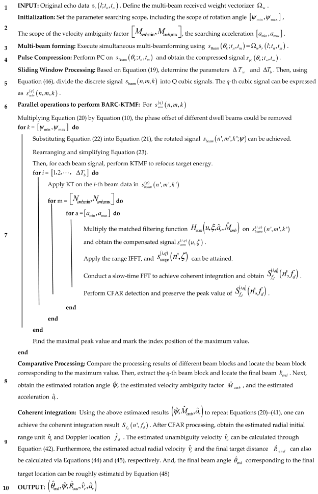
3.3. Detailed Implementation Steps

Generally, the UDAR system will simultaneously construct multiple dwell beams in the azimuth dimension. Full-beam processing brings about extremely high computational complexity. Thereafter, to improve the efficiency of multi-beam processing, we present the sliding windows implementation approach of the proposed method in this subsection. Figure 6a gives the schematic diagram of sliding windows in the beam dimension. By designing the windowing length and interval, small-scale beam cubic data can be extracted. For example, the q-th sliding windows beam cubic data can be given as follows:

$$\begin{array}{cc}{s}_{win}^{\left(q\right)}\left(k,n,m\right)& =A_{1m}\mathrm{sinc}\left\{{\displaystyle \frac{1}{2}}\left[n-n_0-{\displaystyle \frac{v_{r}m{T}_r+0.5a_r{\left(m{T}_r\right)}^2}{\Delta r}}\right]\right\}\exp \left\{-j{\displaystyle \frac{4\pi }{\lambda }}\left[R_0+v_{r}m{T}_r+{\displaystyle \frac{1}{2}}{a}_r{\left(m{T}_r\right)}^2\right]\right\}\hfill \\ & \times \mathrm{rect}\left[{\displaystyle \frac{k-q\Delta T_w}{\Delta T_b}}\right]\mathrm{sinc}\left[-{\displaystyle \frac{\pi Ld\tilde{\eta }\Delta \theta }{4\lambda }}\left(k-k_0-{\displaystyle \frac{\omega m{T}_r}{\Delta \theta }}\right)\right]\exp \left[-j{\displaystyle \frac{\pi d\left(L-1\right)}{\lambda }}\sin \left({\theta }_k\right)\right]\hfill \end{array}$$

(46)

where $\Delta T_w$ is the beam interval of the sliding windows, and $\Delta T_b$ indicates the sliding windows’ length along the beam dimension. If the q-th signal cube contains the target signal spanning multiple beams, the subsequent BARC-KTMF method can achieve the fusion and accumulation of the target energy. Therefore, the variable $\Delta T_b$ needs to be less than the maximum number of beams $\Delta T_{b,\max }$ subject to Equation (19).

After sliding window processing, we can obtain cubic signals of Q divided beam blocks within the K received beams, and the value of Q can be determined by the following:

$$Q=⌊{\displaystyle \frac{K-\Delta T_b}{\Delta T_w}}⌋+1$$

(47)

where $⌊·⌋$ operation represents rounding down to the nearest integer.

Furthermore, the detailed implementation sketch map of the proposed approach is provided in Figure 6b. Next, the parallel operations are performed on different data cubes to improve computational efficiency. In this case, ${\Re }_q\left\{P_0,\psi ,M_{amb},a_r\right\}$ represents the coherent integration result for each beam block. If the q-th beam block contains the target signal spanning multiple beams, the subsequent BARC-KTMF method can achieve the fusion and accumulation of the target energy. Thus, by comparing the peak value, the optimal beam block and estimated parameters can be obtained. In addition, the final angle associated with the final target location can be coarsely estimated as follows:

$${\widehat{\theta }}_{\mathrm{end}}={\theta }_{\min }+(q^{\ast }\Delta T_w+{\widehat{k}}_{end}-1)\cdot \Delta \theta$$

(48)

where ${\theta }_{\min }$ represents the initial angle related to the center of the first dwell beam, and $q^{\ast }$ denotes the beam block within the target energy. The detailed procedures of this implementation approach are listed in Algorithm 1.

Algorithm 1: The detailed procedures of the implementation approach

4. Additional Analysis for the Proposed Approach

In this section, some supplementary discussions for the proposed algorithm are given to verify the performance.

4.1. The Analysis of Computational Complexity

In this subsection, the computational burden of the proposed method is analyzed. Suppose that $N_b$, $N$, and $M$ denote the number of received beams, range units, and echo pulses, respectively. The number of complex multiplications is used to quantify the computational burden. Moreover, only the scenario with a single target is taken into account.

The BARC-KTMF mainly includes beam–domain beam plane rotation and coherent accumulation within the beam. For the full-beam processing, the computational burden of the BARC operation is the order of $O\left(N_{\psi }{N}_{beam}\left(NM{\log }_2\left(M/2\right)+\left(M^2+2M\right)N)\right)\right)$, and the computational burden of the KTMF operation within the beam is the order of $O\left(N_{\psi }{N}_{beam}{N}_{amb}{N}_{a}MN{\log }_2(M/2)\right)$. This algorithm is a three-dimensional search operation for the spatial rotation angle, ambiguity factor, and radial acceleration. Its computational burden is $O\left(N_{\psi }{N}_{beam}\left(NM{\log }_2\left(M/2\right)+\left(M^2+2M\right)N+N_{amb}{N}_{a}MN{\log }_2(M/2)\right)\right)$.

STGRFT [43] requires the extraction operation of the pulse segments where the target is located. Coupled with the three dimensions that the GRFT algorithm itself needs to search, a total of five-dimensional parameter search needs to be carried out, and its computational complexity is of the order of $O\left(N_{beam}{N}_{{\eta }_0}{N}_{{\eta }_1}{N}_v{N}_{a}NM\right)$.

WRFRFT [44] is a six-dimensional parameter search operation that includes the start time, end time, initial radial distance, radial velocity, radial acceleration, and the order of the fractional Fourier transform. The optimal CI performance can be achieved only when the search parameters match the actual target parameters. Therefore, its computational complexity is of the order of $O\left(N_{beam}{N}_{{\eta }_0}{N}_{{\eta }_1}{N}_{\mu }{N}_v{N}_a{N}_{\mathrm{r}}M{\log }_{2}M\right)$.

The MBPCF-MSWPD [45] algorithm first employs the multi-beam phase compensation function (MBPCF) to compensate for the spatial domain phase differences among multiple beams ($O\left(N{N}_a{\log }_{2}M\right)$). Then, it utilizes the multi-scale sliding window function difference technique to extract the time block where the target is located within the beam and complete the accumulation of the target energy ($O\left(N_{{\eta }_0}{N}_{{\eta }_1}\left(NM{\log }_{2}M+NM{\log }_{2}N\right)\right)$). Finally, it uses the spatial projection method to align the target energies from different beams $O\left(C_x{C}_y{C}_{\mathrm{z}}\left(NM{\log }_{2}M\right)\right)$, where $C_x{C}_y{C}_z$ represents the spatial searching grid at the target location. Thus, this method is a six-dimensional searching operation with the order of $O\left(N_{beam}\left(N{N}_a{\log }_{2}M+N_{{\eta }_0}{N}_{{\eta }_1}\left(NM{\log }_{2}M+NM{\log }_{2}N\right)\right)+C_x{C}_y{C}_{\mathrm{z}}\left(NM{\log }_{2}M\right)\right)$.

Based on the above analysis, assume that $N_{beam}=31$, $M=2000$, $N=256$ and other parameter values are equal to $M$. Then, the method in [43] requires around $4.6\times {10}^{12}$ flops, the method in [44] needs the computation burden around $1.5\times {10}^{11}$ flops, and the method in [45] requires around $1.5\times {10}^{11}$ flops. As for the proposed algorithm in this paper, only $4.9\times {10}^9$ flops are needed under the full beam processing, which achieves a three-order-of-magnitude reduction compared with the traditional multidimensional search algorithms [43,44,45]. Therefore, the proposed method significantly improves computational efficiency.

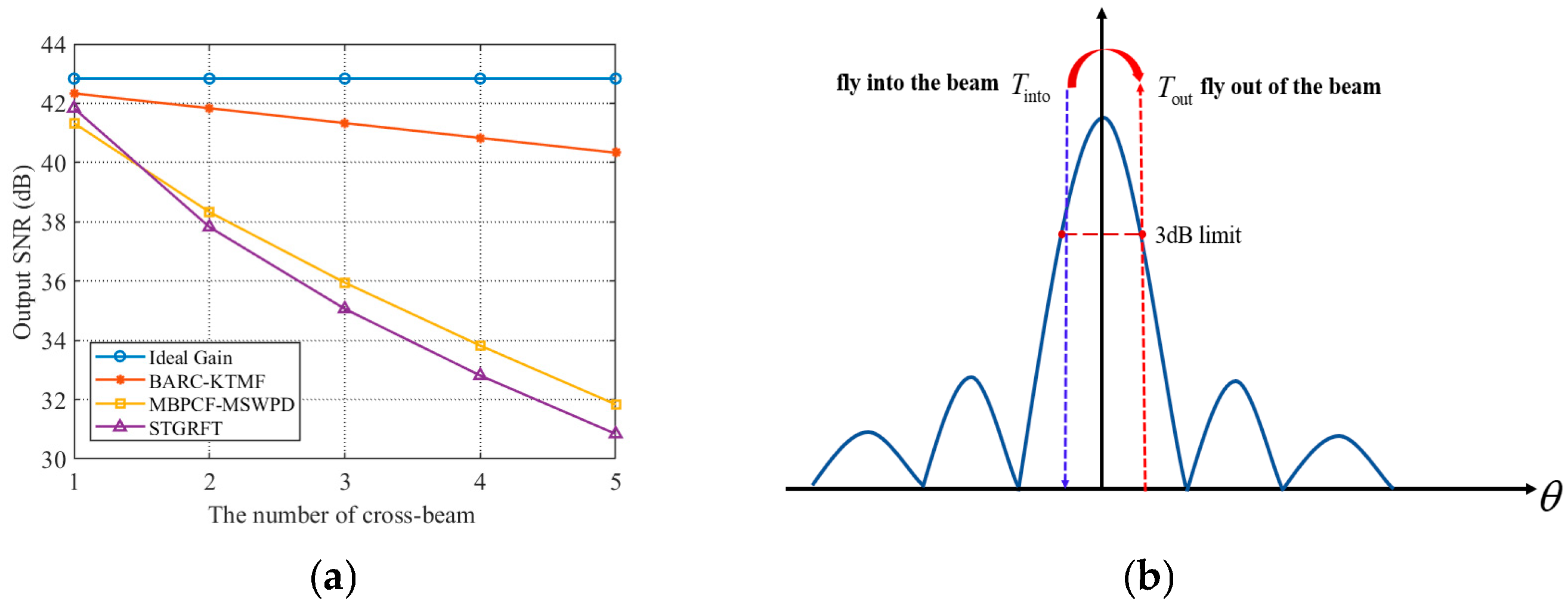
4.2. The Analysis of the Output SNR

In this subsection, the output SNRs under the across-beam situation are analyzed first. Through comparing with several LTCI methods,

Table 1. Output SNRs for different methods.

Methods	Output SNRs	Remarks
Ideal Gain	$SN{R}_{out}=SN{R}_{in}+G_{DBF}+G_{pc}+G_{CI}$	$G_{CI}=10{\log }_{10}\left(N_b\right)+10{\log }_{10}\left(N_p\right)$
BARC-KTMF	$SN{R}_{BARC-KTMF}=SN{R}_{in}+G_{DBF}+G_{pc}+G_{BARC-KTMF}-N_b{L}_b$	$G_{\mathrm{BARC}\text{-}\mathrm{KTMF}}=10{\log }_{10}\left(M\right)+G_{\mathrm{com}}$
MBPCF-MSWPD	$\begin{array}{c}SN{R}_{MBPCF-MSWPD}=SN{R}_{in}+G_{DBF}+G_{pc}+G_{MBPCF-MSWPD}\\ -L_s-N_b{L}_b\end{array}$	$G_{MBPCF-MSWPD}\approx 10{\log }_{10}\left(\sqrt{N_b}\right)+10{\log }_{10}\left(N_p\right)+G_{com}$
STGRFT	$SN{R}_{STGRFT}=SN{R}_{in}+G_{DBF}+G_{pc}+G_{STGRFT}-N_b{L}_b$	$G_{STGRFT}=10{\log }_{10}\left(N_p\right)$

where $SN{R}_{in}$ represents the received echo SNR from the array elements. $G_{DBF}\approx 10{\log }_{10}\left(L\right)$ denotes the energy gain of the DBF operation. $G_{pc}=T_{p}B$ is the PC gain. $N_b$ is the number of across-beam and $N_p$ is the pulse number within the intra-beam. $L_s$ refers to the energy loss resulting from the nonlinear operation. $L_b$ indicates the energy loss resulting from the target crossing multiple beams. $G_{\mathrm{com}}$ indicates the SNR gain by the dwell beam phase compensation.

gives the output SNR results and remarks on the SNR gains of some key steps.

Next, the simulation is executed to display the theoretical output SNR performance based on Table 1. Suppose that there is a high-speed target leading to the across-beam problem. And the important SNR gains and energy loss values are set as follows: $SN{R}_{in}=-30\mathrm{dB}$, $G_{DBF}+G_{pc}=39.8\mathrm{dB}$, $G_{DBF}=16.8\mathrm{dB}$, $M=2000$, $N_p=M/N_b$, $L_s=1\mathrm{dB}$, $L_b=1\mathrm{dB}$, $G_{com}\approx 0.5N_b\mathrm{dB}$. Figure 7a demonstrates the output SNRs with different LTCI algorithms. One can observe that the proposed algorithm is closer to the ideal gain situation. But the integrated performance of the other two algorithms gradually decreases with the increased number of across-beams. It is worth noting that the across-beam effect after spatial beamforming would lead to the accumulated energy loss of DBF operation because the dwell beam fails to precisely point at the time-varying target angle. Moreover, from Figure 7b, when a high-speed target flies into and out of the beam, DBF can be viewed as an incomplete matched filtering operation. In this case, energy loss is difficult to avoid. Therefore, the more beams are crossed, the greater the loss will be.

5. Simulation and Experiment Results

The effectiveness of the proposed method is verified by simulation experiments, including a single-target simulation experiment, a multi-target simulation experiment, a comparative simulation experiment with the existing methods, and a target detection performance experiment. The main radar system parameters are provided in

Table 2. Radar system parameters.

Parameter Name	Symbol	Parameter Value	Parameter Name	Symbol	Parameter Value
Carrier frequency	$f_c$	150 MHz	Pulse duration	$T_p$	10 μs
Bandwidth	$B$	10 MHz	Array element number	$L$	48
Range unit number	$N$	256	Element spacing	$d$	1 m
Pulse repetition frequency	$PRF$	1000 Hz	Receive beam number	$K$	31
Pulse number	$M$	2000	Receive beam range	-	[−30°: 2°: 30°]
Sampling rate	$f_s$	10 MHz	Beam width	$\Delta \theta$	2°

.

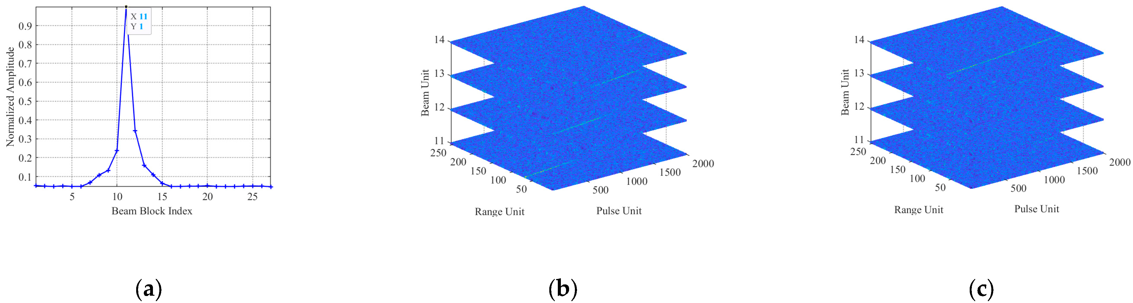
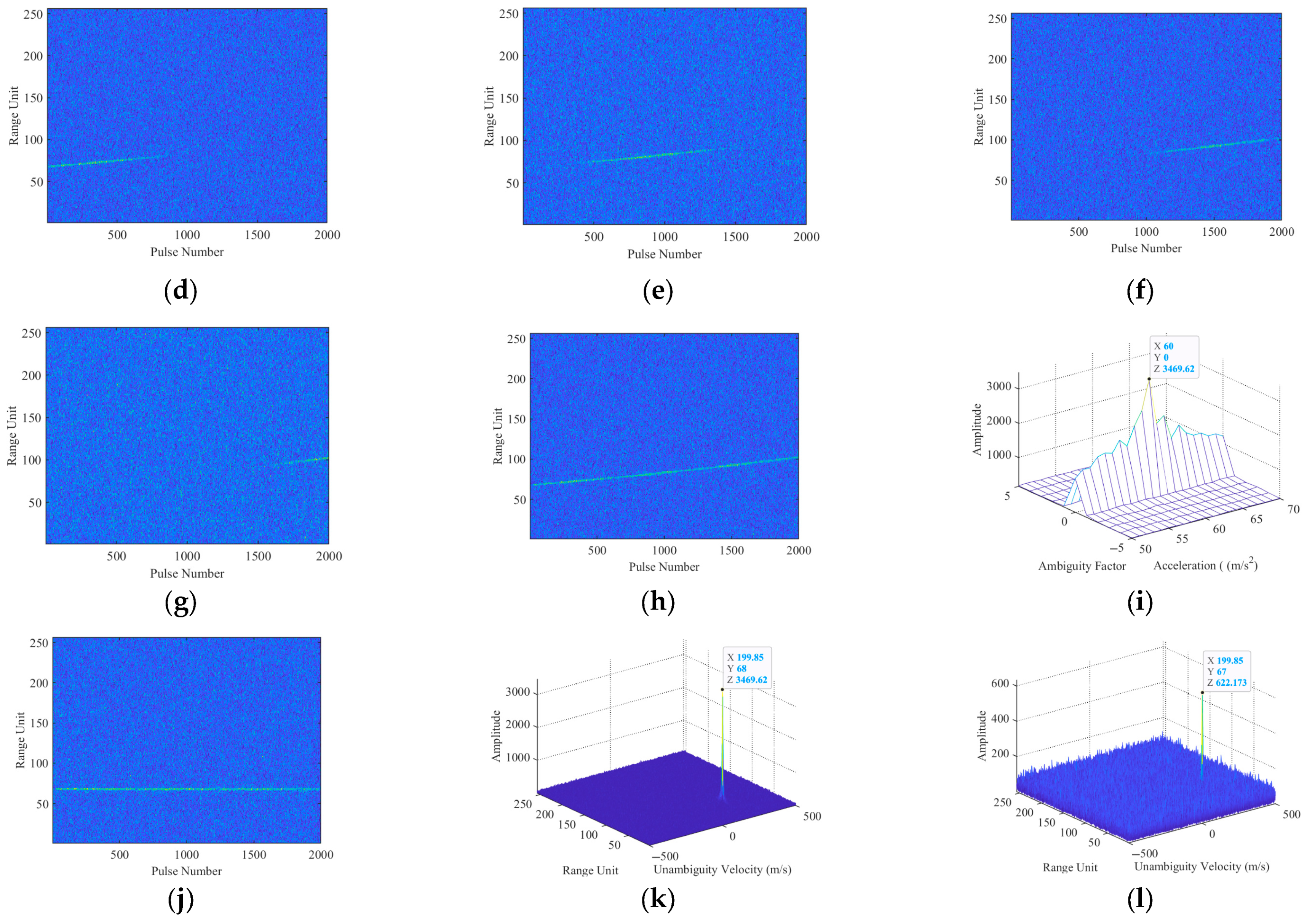
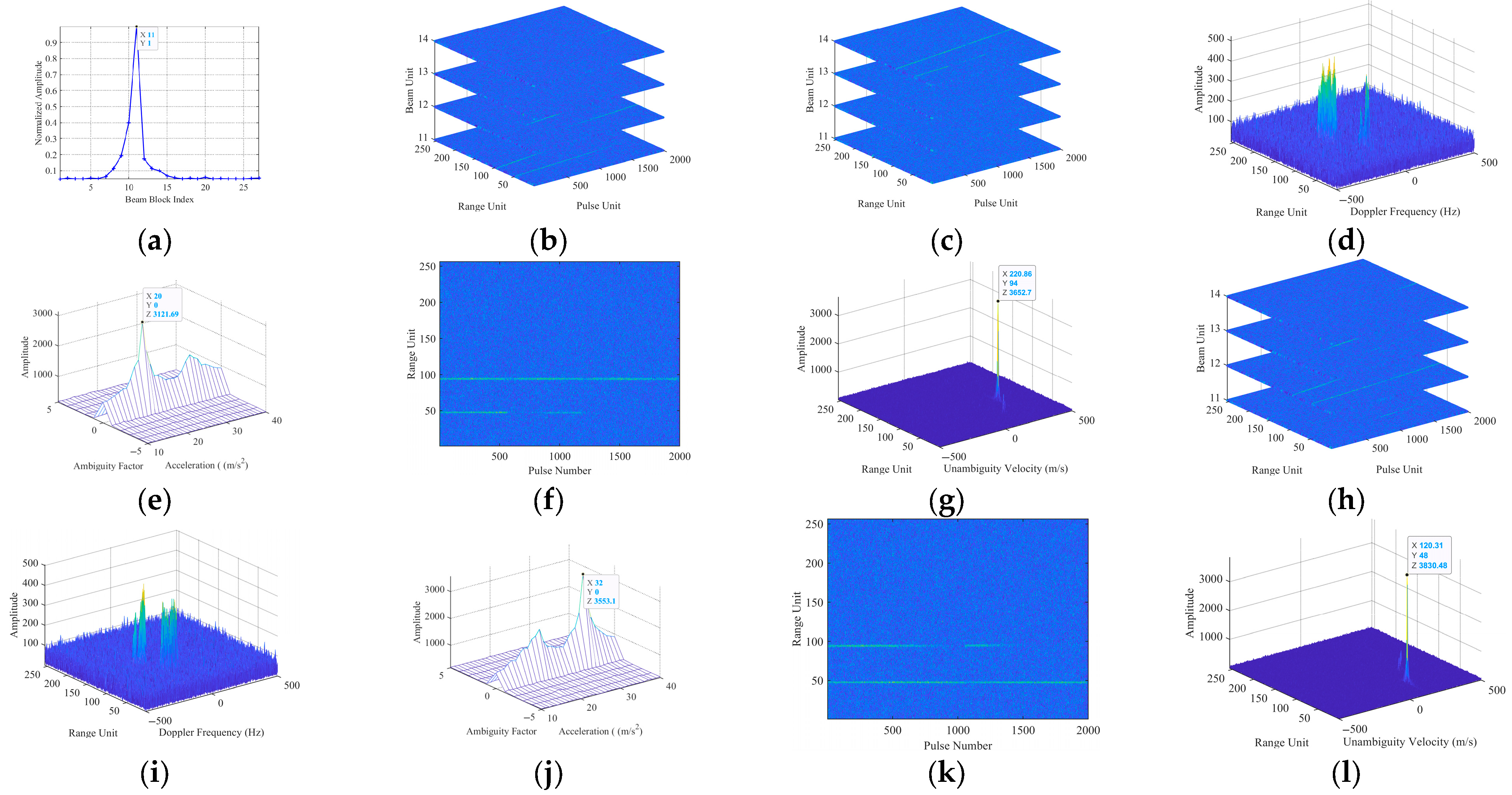
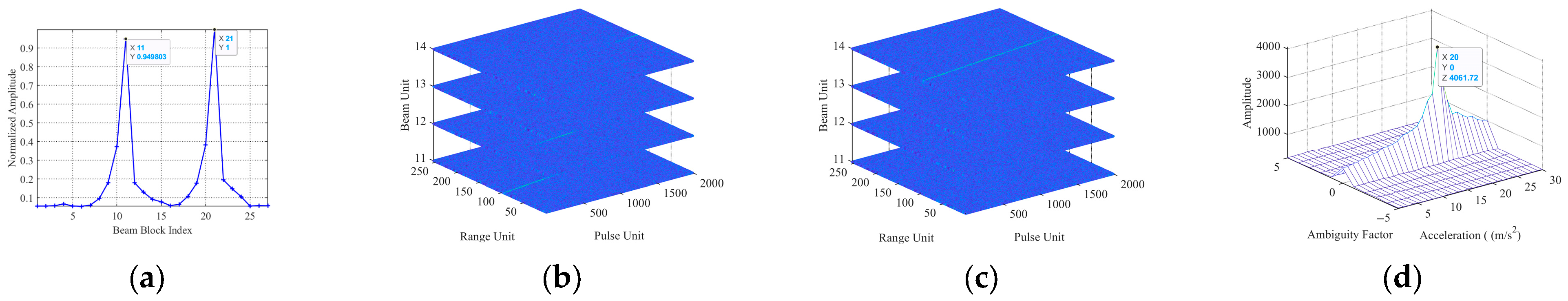
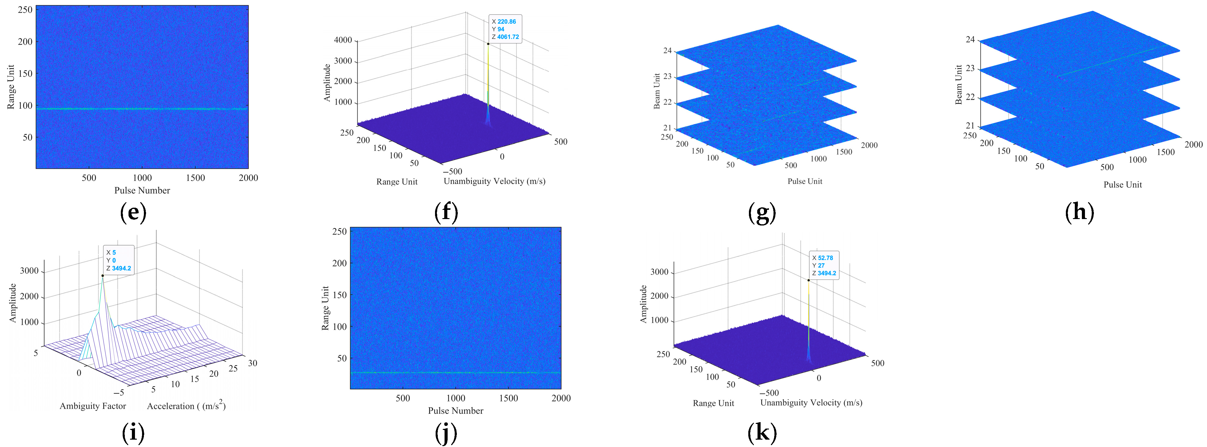
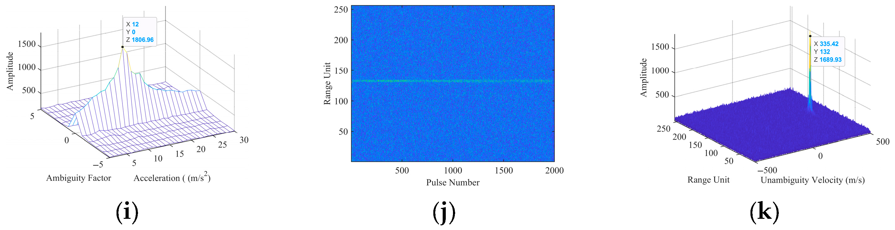
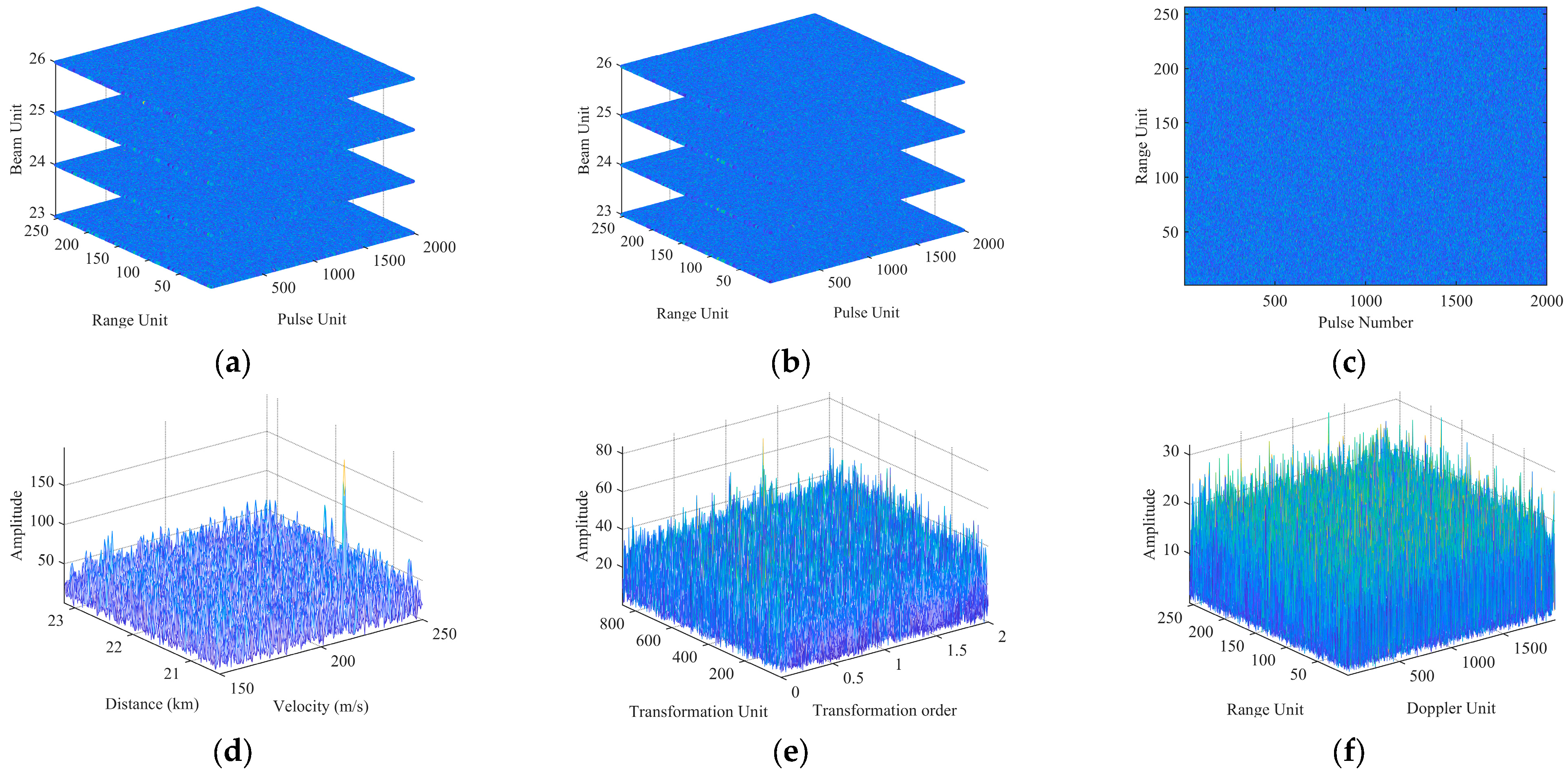
5.1. Single-Target Simulation Experimental Results

To begin with, we perform a single-target simulation experiment to verify the coherent integration and parameter estimation performance. The motion parameters of Target A are listed in

Table 3. The motion parameters of the high-speed Target A.

Parameter Name	Symbol	Target A
Azimuth angular velocity	$\omega$	0.0571 rad/s
Incident angle	${\theta }_0$	−11°
Initial radial range	$R_0$	21,000 m
Radial velocity	$v_r$	200 m/s
Radial acceleration	$a_r$	60 m/s2

. Gaussian white noise with a mean of 0 is adopted in the following simulation experiments, and the SNR before DBF is set as −30 dB. Additionally, the beam interval $\Delta T_w$ and the sliding window length $\Delta T_b$ are set as 1 and 4, respectively.

Through multi-beamforming operation, the original multi-channel echo signal could be transformed into the cubic signal. For each beam channel, pulse compression operation is performed to enhance the signal gain along the range dimension. According to the sliding window, the signal cube would be divided into 27 signal beam blocks, and BARC-KTMF is applied in each beam block to obtain the target signal. Figure 8 shows the detailed single-target simulation results. Specifically, Figure 8a denotes the beam block searching result using the proposed approach, where the 11th beam block can be obtained. Owing to the relationship between $\Delta T_w$ and $\Delta T_b$, the index of the beam unit can be acquired. Then, the original target echoes of the beam domain are distributed in four beams corresponding to the 11th~14th beam units. After the BARC operation, the across-beam signals’ energy can be relocated into the final beam unit in Figure 8c, which is beneficial to obtain the actual target location within the integration time.

Figure 8d–g provide the target trajectory from four beam planes after pulse compression, where the obvious ARU effect occurs in each beam plane and the start/end times of the target path in each beam are different. Given that the target tangential angular velocity is constant, the segmented signals are located in sequential time periods. Next, Figure 8h indicates the extracted final beam slice after the ABU correction. One can see that these segmented signals are reconstructed into an intact target trajectory at the 14th beam. At this point, the ABU issue can be removed, and the across-beam accumulation effectively translates into a traditional intra-beam accumulation task. Moreover, the KTMF method could be used to compensate for ARU and ADU effects. After the 2D matched searching operation, the integrated peak in the velocity ambiguity factor-acceleration searching plane is displayed in Figure 8i, from which the velocity ambiguity factor and acceleration of the target can also be estimated as 0 and 60 m/s², respectively. And then, using the estimated parameters to compensate for the residual range walk and the SRM, the corrected range–pulse echoes can be depicted in Figure 8j, where the target path is concentrated in the same range unit. It means that the ARU effect has been effectively eliminated. Finally, slow-time dimension FFT is utilized to achieve CI, and Figure 8k shows the integrated result within the final beam unit. It can be seen that the target energy can be refocused into an obvious high peak in the range–Doppler plane, which indicates that the ADU issue is also compensated. Therefore, after the proposed approach, ABU, ARU, and ARU can be effectively eliminated, and the target energy can be integrated well. Finally, the motion parameters of this target can be acquired as follows: $\widehat{\omega }$ = 0.0570 rad/s, ${\widehat{\theta }}_{\mathrm{end}}$ = −4°, ${\widehat{R}}_{end}$ = 21,522 m. The above results show that the algorithm can not only compensate for the “three-crossing” issue, but also achieve the coarse estimation of the high-speed target position.

Furthermore, in order to compare the difference before and after the across-beam accumulation, we directly perform the KTMF processing on the segmented signal of the 11th beam, where partial signal energy exists. The accumulation result is shown in Figure 8l. Because the BARC-KTMF can realize the joint coherent integration within the inter-beam, its integrated result is higher than the accumulated value of Figure 8l. The calculation results show that the SNR gain of single-beam processing is 23.5609 dB, while that of multi-beam joint processing reaches 40.1631 dB. Simulation experiments indicate that multi-beam joint processing can significantly improve the SNR gain.

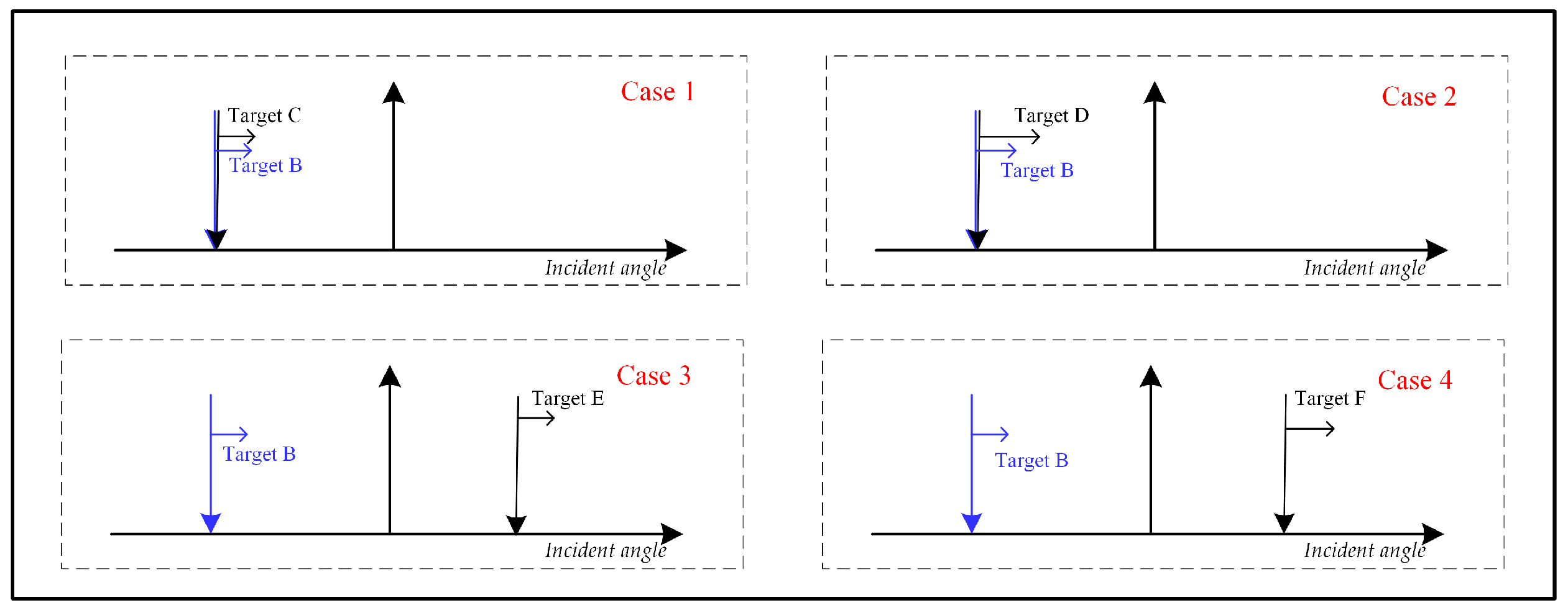
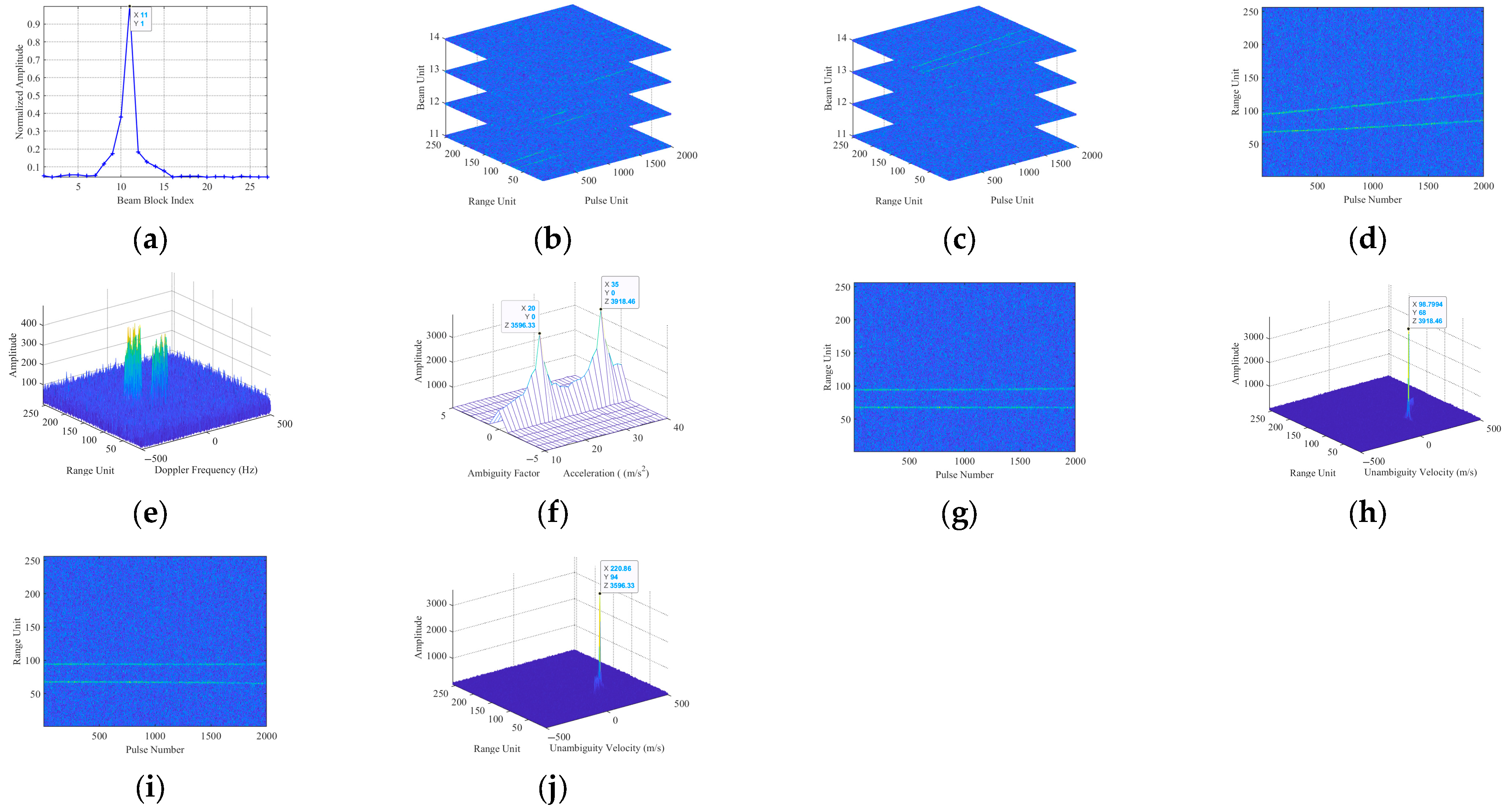
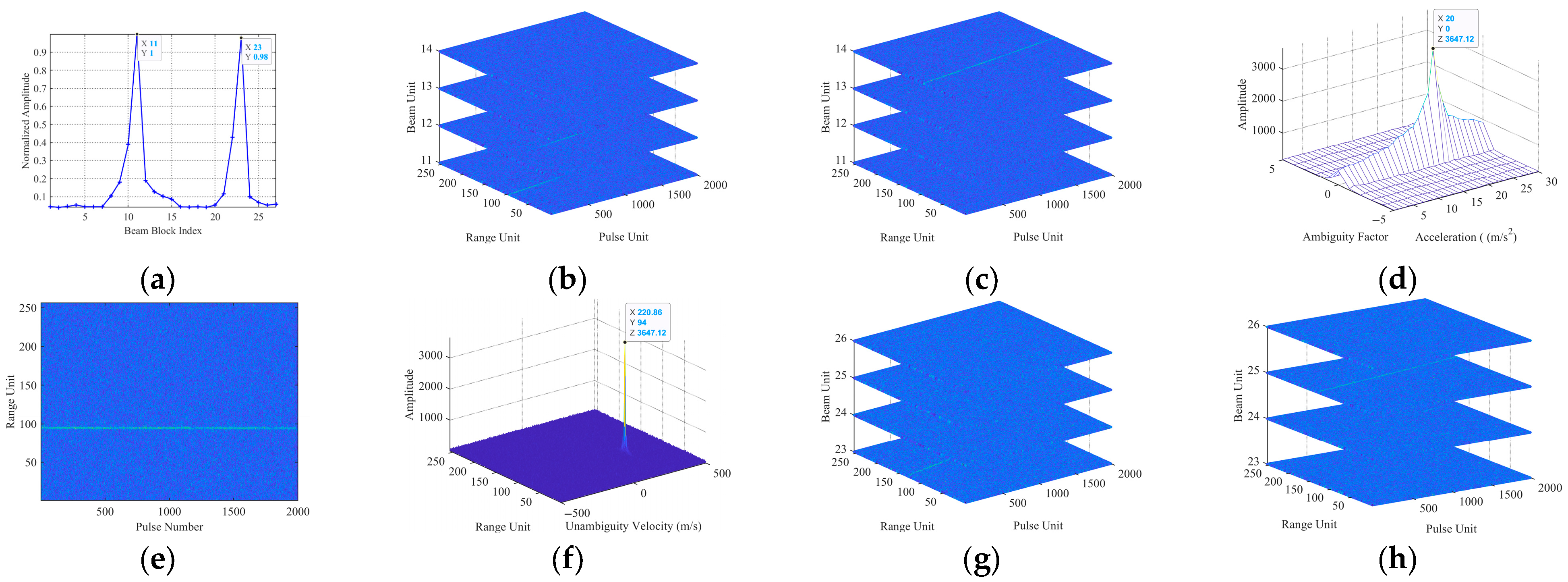
5.2. Multi-Target Simulation Experiment Results

In this subsection, we discuss the multiple-target energy integration performance of the presented algorithm. Given the extensive existing research on the intra-beam multi-target detection, our discussion here specifically emphasizes the spatial domain multi-target integration detection. Thus, considering the target’s tangential kinematic properties, the four scenes, including five targets, are categorized to describe the spatial distribution states of multiple targets. In detail,

Table 4. Multi-target motion parameters.

Parameter Name	Target B	Target C	Target D	Target E	Target F
Azimuth angular velocity	0.057 rad/s	0.057 rad/s	0.029 rad/s	0.057 rad/s	0.046 rad/s
Incident angle	−11°	−11°	−11°	9°	13°
Initial range	21,200 m	20,800 m	20,500 m	20,187 m	21,774 m
Radial velocity	220 m/s	98 m/s	120 m/s	52 m/s	335 m/s
Radial acceleration	20 m/s2	35 m/s2	32 m/s2	5 m/s2	12 m/s2
SNR before DBF	−30 dB	−30 dB	−32 dB	−31 dB	−33 dB

gives the motion parameters of these targets, and Figure 9 shows four cases related to multiple targets.

Case (1): In this scenario, Target B and Target C share identical incident angles (−11°) and tangential angular velocities (0.057 rad/s), resulting in coherent motion within the same beam block (11th–14th beams, Figure 10a). After applying the proposed method, ABU correction aligns both targets to the final beam (Figure 10b–d). At this time, residual ARU/ADU effects disperse energy across range–Doppler units (Figure 10e). Then, KTMF processing resolves radial parameters: acceleration estimation (Figure 10f) enables ARU correction for Target C (Figure 10g) and Target D (Figure 10i), yielding focused Doppler peaks (Figure 10h–j). In addition, the motion parameter of two targets could be estimated as $\left({\widehat{\theta }}_{\mathrm{end},\mathrm{B}}=-4^{\circ },{\widehat{\psi }}_B=0.0571 \mathrm{rad}/\mathrm{s},{\widehat{R}}_{\mathrm{end},\mathrm{B}}=21682 \mathrm{m},{\widehat{v}}_{r,B}=220.86 \mathrm{m}/\mathrm{s},{\widehat{a}}_{r,B}=20{ \mathrm{m}/\mathrm{s}}^2\right)$ and $\left({\widehat{\theta }}_{\mathrm{end},\mathrm{C}}=-4^{\circ },{\widehat{\psi }}_C=0.0571\mathrm{rad}/\mathrm{s},{\widehat{R}}_{\mathrm{end},\mathrm{C}}=21068m,{\widehat{v}}_{r,C}=98.79 \mathrm{m}/\mathrm{s},{\widehat{a}}_{r,C}=35{ \mathrm{m}/\mathrm{s}}^2\right)$, respectively. This case demonstrates that for targets with identical spatial–tangential dynamics, radial parameter differentiation (via KTMF) enables multi-target detection after beam–domain alignment.

Case (2): Target B and Target D share the same incident angle but exhibit distinct tangential angular velocities. As illustrated in Figure 11, this scenario highlights the algorithm’s capability to resolve targets with identical spatial positions but divergent angular motions. Despite their shared incident angle, placing them in the same 11th beam block initially, the targets’ differing angular velocities lead to distinct energy distributions across the beam–time domain. Processing results for Target B (Figure 11b–f) demonstrate successful ABU correction and energy focusing in the final beam unit. As for Target D, several correction results are given in Figure 11h–l, where the across-beam signal energy finally concentrates in the range–Doppler plane to form an obvious integrated peak. It should be noted that due to the small tangential velocity of Target D, its trajectory eventually crosses three beams. Using the beam rotation, signal energy is focused on the 12th beam, as shown in Figure 11h. And the motion parameters of Target D can be estimated as $\left({\widehat{\theta }}_{\mathrm{end},\mathrm{D}}=-4^{\circ },{\widehat{\psi }}_D=0.0287 \mathrm{rad}/\mathrm{s},{\widehat{R}}_{\mathrm{end},\mathrm{D}}=\mathrm{20,805} \mathrm{m},{\widehat{v}}_{r,D}=120.31 \mathrm{m}/\mathrm{s},{\widehat{a}}_{r,D}=32{ \mathrm{m}/\mathrm{s}}^2\right)$. Overall, this case exemplifies multi-target differentiation via rotational angle parameter estimation.

Case (3): In terms of Case 3, Target B (−11°) and Target E (9°) exhibit different incident angles but share the same tangential angular velocity (0.057 rad/s). For Target B, the consistent correction results are listed in Figure 12a–f, respectively. Owing to the spatial difference, the 21st beam block’s signal distribution from Figure 12g reflects the distinct incident angle for Target E and the ABU correction result can be provided in Figure 12h, while the 2D parameter search result (Figure 12i), ARU correction (Figure 12j), and the integrated peak (Figure 12k) confirm the accurate radial parameter estimation. Finally, the estimated motion parameters of Target E can be provided as follows: $\left({\widehat{\theta }}_{\mathrm{end},\mathrm{E}}={14}^{\circ },{\widehat{\psi }}_E=0.0572 \mathrm{rad}/\mathrm{s},{\widehat{R}}_{\mathrm{end},\mathrm{E}}=20303 \mathrm{m},{\widehat{v}}_{r,E}=52.77 \mathrm{m}/\mathrm{s},{\widehat{a}}_{r,E}=5{ \mathrm{m}/\mathrm{s}}^2\right)$. In summary, this case validates that different spatial incident angles (even with identical angular velocities) enable effective multi-target differentiation through beam–domain processing.

Case (4): Case 4 features Target B (−11°, 0.057 rad/s) and Target F (13°, 0.046 rad/s), differing in both incident angles and angular velocities. Similar to Case 3, due to the high spatial distinguishability between the two targets, the windowing method can achieve differentiation of multiple targets. Figure 13a–f shows Target B’s consistent processing in the 11th beam block, while Target F’s trajectory appears in the 23rd beam block from Figure 13g. Figure 13h indicates the beam domain signal distribution after ABU correction, where the whole target signal is shifted into the 25th beam plane corresponding to the ${\widehat{\theta }}_{\mathrm{end},\mathrm{F}}={18}^{\circ }$. Then, the target energy accumulation result along the radial direction is given in Figure 13i–k. Meanwhile, the estimated motion parameters of Target F could be provided as follows: $\left({\widehat{\theta }}_{\mathrm{end},\mathrm{F}}={18}^{\circ },{\widehat{\psi }}_F=0.0289 \mathrm{rad}/\mathrm{s},{\widehat{R}}_{\mathrm{end},\mathrm{F}}=22469 \mathrm{m},{\widehat{v}}_{r,F}=335.46 \mathrm{m}/\mathrm{s},{\widehat{a}}_{r,F}=12{ \mathrm{m}/\mathrm{s}}^2\right)$. In general, for multiple targets with differences in both spatial and radial dimensions, the proposed method can effectively achieve multi-target resolution.

Through the four multi-target scenarios, the proposed approach effectively achieves across-beam energy accumulation and performs coarse estimation of target motion parameters. The algorithm concurrently estimates tangential (angular velocity) and radial (velocity/acceleration) motion characteristics of high-speed targets, validating its versatility in complex beam–domain detection tasks.

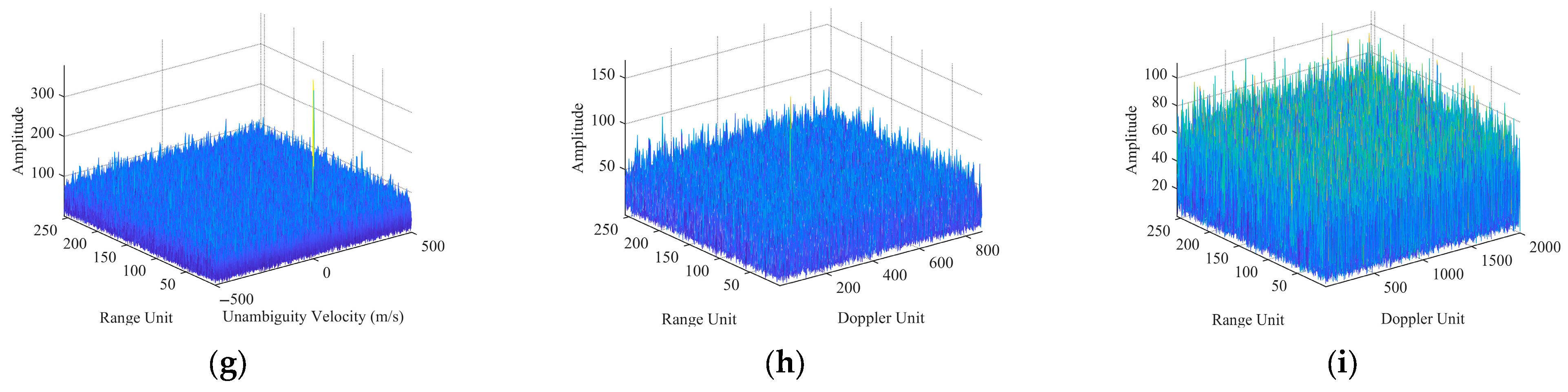
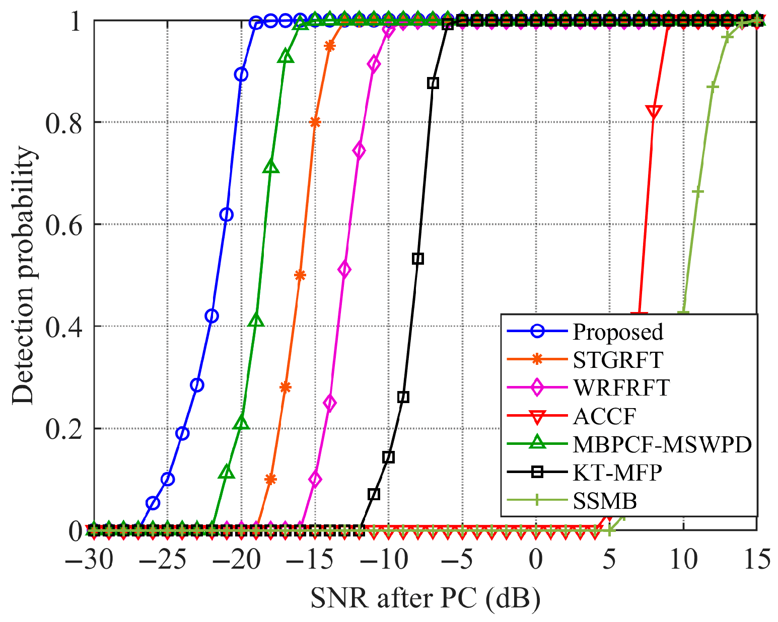
5.3. Comparisons with the Existing Methods Under Low SNR

Further, to demonstrate the accumulation capability of the proposed method under low SNR conditions. In this subsection, several algorithms are compared to verify the integration performance. The radar system parameters are the same as those in Table 2. And the main target motion parameters are the same as Target F in Section 5.2. Especially, the initial SNR of element-level received echoes is set to −50 dB, and the target path has crossed three beam units. As shown in Figure 14a, the target echo is completely submerged in the noise background in the corresponding 23rd beam block because of the low signal energy. Figure 14b,c further shows the beam domain correction results, and the target trajectory is still difficult to detect.

Next, we compare the accumulation performance differences between single-beam processing and multi-beam processing. The essence of STGRFT [43] is to achieve intra-segment target energy accumulation using GRFT after matching the optimal time interval where the target is located. Similarly, the WRFRFT [44] method obtains the optimal window function through searching, and then accumulates target signals in the transform domain via the FRFT method. However, limited by the actual signal length of the target within the beam after across-beam processing, the accumulation performance of the above methods is restricted. Nonlinear operations in the ACCF [13] algorithm introduce noise energy, resulting in its failure to effectively accumulate target energy under low SNR conditions, and the echo signal is overwhelmed by noise. Figure 14d,e show the accumulation results of [13,43,44] for the proposed method, respectively. According to statistical results, the output SNRs of the STGRFT and WRFRFT are 13.5986 dB and 11.0678 dB, respectively, while the output SNR of the proposed method reaches 19.0777 dB. Thus, simulation experiments show that multi-beam joint processing can significantly improve the SNR gain.

Secondly, the performances of two multi-beam accumulation methods are displayed as well. Figure 14h gives the non-coherent accumulation result of the MBPCF-MSWPD [45] method corresponding to an output SNR of 16.0486 dB, which has inferior performance to that of multiple beams coherent accumulation. Additionally, since the SSMB [42] method does not compensate for the ARU and ADU effects within the beam, it incurs significant performance degradation from Figure 14i. Overall, compared with existing typical LTCI algorithms [13,42,43,44,45], the proposed algorithm demonstrates excellent cross-beam signal accumulation capability under a low SNR scenario.

5.4. Target Detection Performance Analysis

To evaluate the noise resistance of the proposed method, a comparative analysis of target detection performance is conducted in this subsection. For ease of analysis, single-target Monte Carlo simulation experiments are performed for illustration, and the radar system parameters are the same as those in Table 2, and the high-speed target motion parameters are set to the same as those in Table 3. The false alarm rate $P_{fa}$ is set to ${10}^{-6}$. The SNR after pulse compression is varied from −30 dB to 15 dB in steps of 1 dB. For each SNR value, 200 Monte Carlo experiments are performed.

Figure 15 shows the variation results of the detection probability against the SNR with different algorithms, including STGRFT [43], WRFRFT [44], KT-MFP [33], ACCF [13], MBPCF-MSWPD [45], SSMB [42], and the proposed method. It should be noted that among the above algorithms, the first four methods are primarily used for the intra-beam signal integration, while the latter three are employed for the inter-beam target energy accumulation. From Figure 15, for the detection probability corresponding to 0.9, the proposed method demonstrates the gain improvements of 3 dB, 5.5 dB, 8 dB, and 13 dB, compared with [33,43,44,45], respectively. As a whole, the proposed method performs better in terms of CI ability than other algorithms because the energy originally dispersed across multiple beams is refocused on the same beam. Specifically, ref. [45] involves the nonlinear operations within the intra-beam and NCI within the inter-beam, leading to signal accumulation loss. Its accumulation performance is weaker than that of the proposed algorithm but stronger than [13,33,43,44], which only aggregates the single beam energy. Meanwhile [42], ignores the ARU correction and ADU elimination within the intra-beam, causing poor detection performance. Therefore, the simulation results of single target and Monte Carlo trials show the advanced performance of the proposed method.

6. Discussions

To enhance the performance of the proposed method, this study summarizes the critical challenges in the across-beam scenario, which will serve as the focal points for future research. These challenges are as follows:

High computational complexity: The algorithm entails multiple intricate computational procedures, including spatial domain beam angle search, three-dimensional coordinate axis rotation, and KTMF processing. This results in a substantial computational load, potentially degrading the algorithm’s real-time performance. In applications with stringent real-time requirements, such as rapid-response air defense systems, high-performance computing resources are often indispensable to meet the processing demands.

Significant dependence on prior information: The algorithm’s performance exhibits considerable reliance on target prior information, such as the initial incident angle. Inaccurate or missing prior information can compromise the precision of three-dimensional coordinate axis rotation, velocity ambiguity factor estimation, and acceleration determination. Consequently, this diminishes the algorithm’s effectiveness in target energy accumulation and motion state estimation, thereby affecting the accuracy of target detection and tracking.

Challenges of high-order tangential motion model: The current algorithm assumes that the tangential motion of the target has a uniform angular velocity ($\omega$ is a constant). However, actual high-speed targets may have an angular acceleration (such as $\omega \left(t\right)={\omega }_0+\alpha t$) or nonlinear angular changes, resulting in non-uniform diffusion of the target energy in the beam domain, and the linear angular rotation compensation method may fail.

Limitations of beam domain processing: The algorithm primarily operates in the beam domain and imposes specific requirements on beam division and coverage. Unreasonable beam division or targets located at the beam edge can undermine the target energy correction and accumulation, leading to reduced target detection performance. Moreover, the algorithm’s performance varies with different beam widths and pointing directions, necessitating optimization and adjustment tailored to specific application scenarios.

7. Conclusions

In this paper, a novel BARC-KTMF approach is presented to achieve across-beam target energy accumulation. This method has the following advantages:

(1)

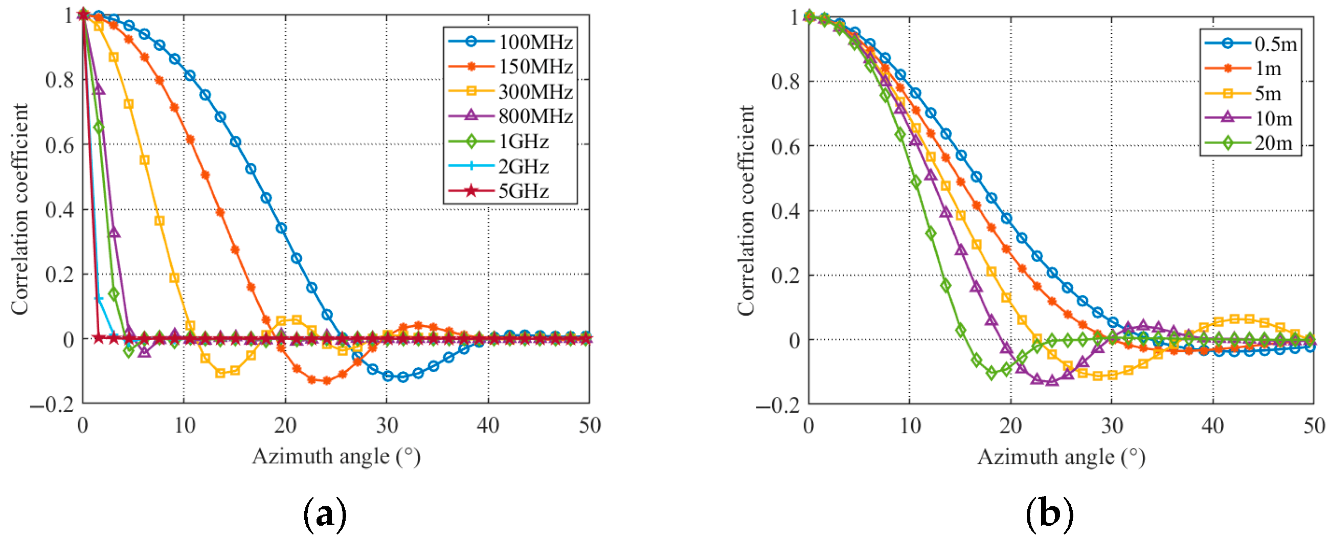
An across-beam 3D signal model for a high-speed target with UDAR system is established to introduce “three-crossing” problems, and the detailed mathematical analysis is conducted on the constraint conditions of the ABU, ARU, and ADU effects. In addition, the multiple perspectives echo correlation experiment shows that the higher the frequency band, the greater the loss of echo correlation.

(2)

Compared with the representative LTCI methods that only perform radial parameter estimation, by utilizing a three-dimensional search based on the spatial domain angle, ambiguity factor, and radial angular velocity, the proposed algorithm realizes excellent accumulation ability, and the tangential and radial motion characteristics of high-speed targets can be obtained.

(3)

We develop a kind of spatial windowing processing approach to accelerate the computational efficiency with multiple beam blocks. Owing to the flexible division of beam blocks, simulation experiments verify that the proposed algorithm possesses the ability to distinguish multiple targets in the spatial domain.

(4)

Moreover, the proposed algorithm effectively corrects the across-beam signal to the final beam unit. It can output angle information that is closer to the true spatial position of the target when the target flies out of the illumination area, which is particularly critical in complex scenarios for high-speed target detection.

In summary, the results of the numerical simulation experiments verify the effectiveness and reliability of the proposed algorithm.

References

1. Hussain, M.; Ahmed, R.; Cheema, H.M. Segmented Radon Fourier Transform for Long-Time Coherent Radars. IEEE Sens. J. 2023, 23, 9582–9594. [Google Scholar] [CrossRef]
2. Xu, J.; Peng, Y.; Xia, X. Focus-before-detection radar signal processing: Part I—Challenges and methods. IEEE Trans. Aerosp. Electron. Syst. 2017, 32, 48–59. [Google Scholar] [CrossRef]
3. Zhang, H.; Liu, W.; Zhang, Q.; Zhang, L.; Liu, B.; Xu, H.-X. Joint Power, Bandwidth, and Subchannel Allocation in a UAV-Assisted DFRC Network. IEEE Internet Things J. 2025, 12, 11633–11651. [Google Scholar] [CrossRef]
4. Zhang, H.; Liu, W.; Zhang, Q.; Liu, B. Joint Customer Assignment, Power Allocation, and Subchannel Allocation in a UAV-Based Joint Radar and Communication Network. IEEE Internet Things J. 2024, 11, 29643–29660. [Google Scholar] [CrossRef]
5. Zhou, X.; Wang, P.; Zeng, H.; Chen, J. Moving Target Detection Using GNSS-Based Passive Bistatic Radar. IEEE Trans. Geosci. Remote Sens. 2022, 60, 3356. [Google Scholar] [CrossRef]
6. Li, D.; Zhan, M.; Liu, H.; Liao, G. A robust translational motion compensation method for ISAR imaging based on keystone transform and fractional Fourier transform under low SNR environment. IEEE Trans. Aerosp. Electron. Syst. 2017, 53, 2140–2156. [Google Scholar] [CrossRef]
7. Liu, G.; Tian, Y.; Wen, B.; Liu, C. Combined Coherent and Non-Coherent Long-Time Integration Method for High-Speed Target Detection Using High-Frequency Radar. Remote Sens. 2024, 16, 2139. [Google Scholar] [CrossRef]
8. Zhang, H.; Liu, W.; Zhang, Q.; Fei, T. A Robust Joint Frequency Spectrum and Power Allocation Strategy in a Coexisting Radar and Communication System. Chin. J. Aeronaut. 2024, 37, 393–409. [Google Scholar] [CrossRef]
9. De Quevedo, A.D.; Urzaiz, F.I.; Menoyo, J.G.; Lopez, A.A. Drone Detection and RCS Measurements with Ubiquitous Radar. In Proceedings of the 2018 International Conference on Radar, Brisbane, Australia, 27–31 August 2018; IEEE: Piscataway, NJ, USA, 2018; pp. 1–6. [Google Scholar]
10. Massardo, M.; Stallone, R. Experimental Validation of a Frustum of Cone Antenna Applied to Omega 360 Ubiquitous 2D Radar. In Proceedings of the 2017 IEEE International Workshop on Metrology for AeroSpace, Padua, Italy, 21–23 June 2017; IEEE: Piscataway, NJ, USA, 2017; pp. 36–39. [Google Scholar]
11. Zheng, J.; Su, T.; Zhu, W.; He, X.; Liu, Q.H. Radar High-Speed Target Detection Based on the Scaled Inverse Fourier Transform. IEEE J. Sel. Top. Appl. Earth Obs. Remote Sens. 2014, 8, 1108–1119. [Google Scholar] [CrossRef]
12. Zheng, J.; Su, T.; Liu, H.; Liao, G.; Liu, Z.; Liu, Q.H. Radar High-Speed Target Detection Based on the Frequency-Domain Deramp-Keystone Transform. IEEE J. Sel. Top. Appl. Earth Obs. Remote Sens. 2016, 9, 285–294. [Google Scholar] [CrossRef]
13. Li, X.; Cui, G.; Yi, W.; Kong, L. A Fast Maneuvering Target Motion Parameters Estimation Algorithm Based on ACCF. IEEE Signal Process. Lett. 2015, 22, 270–274. [Google Scholar] [CrossRef]
14. Li, X.; Cui, G.; Yi, W.; Kong, L. Sequence-Reversing Transform-Based Coherent Integration for High-Speed Target Detection. IEEE Trans. Aerosp. Electron. Syst. 2017, 53, 1573–1580. [Google Scholar] [CrossRef]
15. Wan, J.; He, Z.; Tan, X.; Li, D.; Liu, H.; Shu, Y.; Chen, Z. Coherent Integration for Maneuvering Target Detection via Fast Nonparametric Estimation Method. Signal Process. 2023, 203, 108820. [Google Scholar] [CrossRef]
16. Niu, Z.; Zheng, J.; Su, T.; Zhang, J. Fast Implementation of Scaled Inverse Fourier Transform for High-speed Radar Target Detection. Electron. lett. 2017, 53, 1142–1144. [Google Scholar] [CrossRef]
17. Huang, P.; Liao, G.; Yang, Z.; Xia, X.-G.; Ma, J.-T.; Ma, J. Long-Time Coherent Integration for Weak Maneuvering Target Detection and High-Order Motion Parameter Estimation Based on Keystone Transform. IEEE Trans. Signal Process. 2016, 64, 4013–4026. [Google Scholar] [CrossRef]
18. Rao, X.; Tao, H.; Su, J.; Guo, X.; Zhang, J. Axis Rotation MTD Algorithm for Weak Target Detection. Digit. Signal Process. 2014, 26, 81–86. [Google Scholar] [CrossRef]
19. Wang, L.; Tao, H.; Yang, A.; Yang, F. Coherent Integration Method for High-speed Target Detection Using Angular Inverse Rotation Transform. Electron. lett. 2024, 60, e70087. [Google Scholar] [CrossRef]
20. Sun, Z.; Li, X.; Yi, W.; Cui, G.; Kong, L. A Coherent Detection and Velocity Estimation Algorithm for the High-Speed Target Based on the Modified Location Rotation Transform. IEEE J. Sel. Top. Appl. Earth Obs. Remote Sens. 2018, 11, 2346–2361. [Google Scholar] [CrossRef]
21. Huang, X.; Zhang, Y.; Zhang, L.; Chen, Z.; Zhang, L. Detection and Fast Motion Parameter Estimation for Target with Range Walk Effect Based on New Axis Rotation Moving Target Detection. Digit. Signal Process. 2022, 120, 103274. [Google Scholar] [CrossRef]
22. Xu, J.; Yu, J.; Peng, Y.-N.; Xia, X.-G. Radon-Fourier Transform for Radar Target Detection, I: Generalized Doppler Filter Bank. IEEE Trans. Aerosp. Electron. Syst. 2011, 47, 1186–1202. [Google Scholar] [CrossRef]
23. Xu, J.; Yan, L.; Zhou, X.; Long, T.; Xia, X.-G.; Wang, Y.-L.; Farina, A. Adaptive Radon–Fourier Transform for Weak Radar Target Detection. IEEE Trans. Aerosp. Electron. Syst. 2018, 54, 1641–1663. [Google Scholar] [CrossRef]
24. Zhu, D.; Li, Y.; Zhu, Z. A Keystone Transform Without Interpolation for SAR Ground Moving-Target Imaging. IEEE Geosci. Remote Sens. Lett. 2007, 4, 18–22. [Google Scholar] [CrossRef]
25. Xu, J.; Xia, X.-G.; Peng, S.-B.; Yu, J.; Peng, Y.-N.; Qian, L.-C. Radar Maneuvering Target Motion Estimation Based on Generalized Radon-Fourier Transform. IEEE Trans. Signal Process. 2012, 60, 6190–6201. [Google Scholar] [CrossRef]
26. Chen, X.; Guan, J.; Liu, N.; He, Y. Maneuvering Target Detection via Radon-Fractional Fourier Transform-Based Long-Time Coherent Integration. IEEE Trans. Signal Process. 2014, 62, 939–953. [Google Scholar] [CrossRef]
27. Chen, X.; Guan, J.; Huang, Y.; Liu, N.; He, Y. Radon-Linear Canonical Ambiguity Function-Based Detection and Estimation Method for Marine Target With Micromotion. IEEE Trans. Geosci. Remote Sens. 2015, 53, 2225–2240. [Google Scholar] [CrossRef]
28. Deng, J.; Sun, Z.; Liu, W.; Li, X.; Cui, G. Blind Source Separation-Based High-Speed Weak Target Coherent Detection Method Under Strong Target BSSL Covering Situation. IEEE Trans. Aerosp. Electron. Syst. 2025, 61, 7987–7994. [Google Scholar] [CrossRef]
29. Li, X.; Sun, Z.; Yi, W.; Cui, G.; Kong, L. Radar Detection and Parameter Estimation of High-Speed Target Based on MART-LVT. IEEE Sens. J. 2019, 19, 1478–1486. [Google Scholar] [CrossRef]
30. Rao, X.; Tao, H.; Xie, J.; Su, J.; Li, W. Long-time Coherent Integration Detection of Weak Manoeuvring Target via Integration Algorithm, Improved Axis Rotation Discrete chirp-Fourier Transform. IET Radar. Sonar. Amp. Navig. 2015, 9, 917–926. [Google Scholar] [CrossRef]
31. Rao, X.; Tao, H.; Su, J.; Xie, J.; Zhang, X. Detection of Constant Radial Acceleration Weak Target via IAR-FRFT. IEEE Trans. Aerosp. Electron. Syst. 2015, 51, 3242–3253. [Google Scholar] [CrossRef]
32. Zeng, C.; Li, D.; Luo, X.; Song, D.; Liu, H.; Su, J. Ground Maneuvering Targets Imaging for Synthetic Aperture Radar Based on Second-Order Keystone Transform and High-Order Motion Parameter Estimation. IEEE J. Sel. Top. Appl. Earth Obs. Remote Sens. 2019, 12, 4486–4501. [Google Scholar] [CrossRef]
33. Sun, Z.; Li, X.; Yi, W.; Cui, G.; Kong, L. Detection of Weak Maneuvering Target Based on Keystone Transform and Matched Filtering Process. Signal Process. 2017, 140, 127–138. [Google Scholar] [CrossRef]
34. Zhan, M.; Huang, P.; Zhu, S.; Liu, X.; Liao, G.; Sheng, J.; Li, S. A Modified Keystone Transform Matched Filtering Method for Space-Moving Target Detection. IEEE Trans. Geosci. Remote Sens. 2022, 60, 1–16. [Google Scholar] [CrossRef]
35. Wang, J.; Zhang, Y. An Airborne SAR Moving Target Imaging and Motion Parameters Estimation Algorithm With Azimuth-Dechirping and the Second-Order Keystone Transform Applied. IEEE J. Sel. Top. Appl. Earth Obs. Remote Sens. 2015, 8, 3967–3976. [Google Scholar]
36. Zhang, Q.; Zhang, Y.; Sun, B.; Dong, Z.; Yu, L. Motion Parameters Estimation and HRRP Reconstruction of Maneuvering Weak Target for Wideband Radar Based on SKT-ELVD. IEEE Trans. Aerosp. Electron. Syst. 2023, 59, 2752–2763. [Google Scholar] [CrossRef]
37. Fang, X.; Xiao, G.; Cao, Z.; Min, R.; Pi, Y. Migration Correction Algorithm for Coherent Integration of Low-Observable Target with Uniform Radial Acceleration. IEEE Trans. Instrum. Meas. 2021, 70, 1–13. [Google Scholar] [CrossRef]
38. Wang, L.; Tao, H.; Yang, A.; Yang, F.; Wang, X. A Fast Non-Searching Method for Maneuvering Weak Target Detection Using Ubiquitous Radar. In Proceedings of the 2023 6th International Conference on Information Communication and Signal Processing, Xi’an, China, 23–25 September 2023; IEEE: Piscataway, NJ, USA, 2023; pp. 512–516. [Google Scholar]
39. Lin, L.; Sun, G.; Cheng, Z.; He, Z. Long-Time Coherent Integration for Maneuvering Target Detection Based on ITRT-MRFT. IEEE Sens. J. 2020, 20, 3718–3731. [Google Scholar] [CrossRef]
40. Zheng, J.; Liu, H.; Liu, J.; Du, X.; Liu, Q.H. Radar High-Speed Maneuvering Target Detection Based on Three-Dimensional Scaled Transform. IEEE J. Sel. Top. Appl. Earth Obs. Remote Sens. 2018, 11, 2821–2833. [Google Scholar] [CrossRef]
41. Huang, P.; Xia, X.-G.; Liu, X.; Liao, G. Refocusing and Motion Parameter Estimation for Ground Moving Targets Based on Improved Axis Rotation-Time Reversal Transform. IEEE Trans. Comput. Imaging 2018, 4, 479–494. [Google Scholar] [CrossRef]
42. Rao, X.; Sun, Z.Y.; Tao, H.H. Multi-Beam Associated Coherent Integration Algorithm for Weak Target Detection. Radioengineering 2024, 33, 1–11. [Google Scholar] [CrossRef]
43. Li, X.; Sun, Z.; Yeo, T.S.; Zhang, T.; Yi, W.; Cui, G.; Kong, L. STGRFT for Detection of Maneuvering Weak Target with Multiple Motion Models. IEEE Trans. Signal Process. 2019, 67, 1902–1917. [Google Scholar] [CrossRef]
44. Li, X.; Sun, Z.; Zhang, T.; Yi, W.; Cui, G.; Kong, L. WRFRFT-Based Coherent Detection and Parameter Estimation of Radar Moving Target with Unknown Entry/Departure Time. Signal Process. 2020, 166, 107228. [Google Scholar] [CrossRef]
45. Hu, R.; Li, D.; Wan, J.; Kang, X.; Liu, Q.; Chen, Z.; Yang, X. Integration and Detection of a Moving Target with Multiple Beams Based on Multi-Scale Sliding Windowed Phase Difference and Spatial Projection. Remote Sens. 2023, 15, 4429. [Google Scholar] [CrossRef]
46. Wang, L.; Tao, H.; Yang, A.; Yang, F.; Ma, H.; Su, J. Radar High-Speed Moving Target Coherent Integration and Parameter Estimation Algorithm Using PSA-FAIR-NUFFT. IEEE Sens. J. 2025, 25, 24712–24730. [Google Scholar] [CrossRef]
47. Niu, Z. Research on Energy Focusing and Detection Technology of Range Migrating Radar Target; Xidian University: Xi’an, China, 2020. [Google Scholar]
Figure 1. System model between a UDAR system and a high-speed target.
Remotesensing 17 02597 g001
Figure 2. The sketch map of the 3D signal model.
Remotesensing 17 02597 g002
Figure 3. The beam segmentation characteristics.
Remotesensing 17 02597 g003
Figure 4. Correlation coefficient curve: (a) The influence of carrier frequency on the correlation coefficient curve. (b) The influence of target shape on the correlation coefficient curve.
Remotesensing 17 02597 g004
Figure 5. The signal processing framework of the proposed approach.
Remotesensing 17 02597 g005
Figure 6. (a) The schematic diagram of sliding windows in the beam dimension. (b) The detailed implementation sketch map of the proposed approach.
Remotesensing 17 02597 g006
Figure 7. (a) The output SNRs against the number of across-beams. (b) Across-beam loss effect.
Remotesensing 17 02597 g007
Figure 8. Single target processing results. (a) Beam block searching result. (b) The original signal distribution map. (c) The corrected signal distribution map. (d) Range–pulse map of the 11th beam. (e) Range–pulse map of the 12th beam. (f) Range–pulse map of the 13th beam. (g) Range–pulse map of the 14th beam. (h) The beam domain correction result of the 14th beam. (i) The velocity ambiguity factor-acceleration searching result. (j) The ARU correction result. (k) The final coherent integrated result. (l) The coherent integrated result of the original 11th beam.
Remotesensing 17 02597 g008aRemotesensing 17 02597 g008b
Figure 9. Four cases related to multiple targets.
Remotesensing 17 02597 g009
Figure 10. Output results for case 1. (a) The beam block index. (b) Beam domain signal distribution of the 11th beam block. (c) The beam domain correction result of two targets. (d) Range compression signals for two targets. (e) Range–Doppler map for two targets without correction. (f) The 2D parameter searching result. (g) The ARU correction result of Target C. (h) The integrated peak of Target C. (i) The ARU correction result of Target B. (j) The integrated peak of Target B.
Remotesensing 17 02597 g010
Figure 11. Output results for case 2. (a) The beam block index. (b) Beam domain signal distribution of the 11th beam block. (c) The beam domain correction result of Target B. (d) Range–Doppler map without correction. (e) The 2D searching result of Target B. (f) The ARU correction result of Target B. (g) The integrated peak of Target B. (h) The ABU correction result of Target D. (i) Range–Doppler map without correction. (j) The 2D parameter searching result of Target D. (k) The ARU correction result of Target D. (l) The integrated peak of Target D.
Remotesensing 17 02597 g011
Figure 12. Output results for case 3. (a) Beam block index. (b) Signal distribution of the 11th beam block. (c) The ABU correction result of Target B. (d) The 2D searching result of Target B. (e) The ARU correction result of Target B. (f) The integrated peak of Target B. (g) Signal distribution of the 21st beam block. (h) The ABU correction result of Target E. (i) The 2D parameter searching result of Target E. (j) The ARU correction result of Target E. (k) The integrated peak of Target E.
Remotesensing 17 02597 g012aRemotesensing 17 02597 g012b
Figure 13. Output results for case 4. (a) Beam block index. (b) Signal distribution of the 11th beam block. (c) The ABU correction result of Target B. (d) The 2D searching result of Target B. (e) The ARU correction result of Target B. (f) The integrated peak of Target B. (g) Signal distribution of the 23rd beam block. (h) The ABU correction result of Target F. (i) The 2D parameter searching result of Target F. (j) The ARU correction result of Target F. (k) The integrated peak of Target F.
Remotesensing 17 02597 g013aRemotesensing 17 02597 g013b
Figure 14. Processing results of six methods. (a) The beam domain signal distribution. (b) The corrected signal distribution. (c) The range–pulse signal slice. (d) The integrated result of the STGRFT method. (e) The integrated result of the WRFRFT method. (f) The integrated result of the ACCF method. (g) The integrated result of the proposed method. (h) The integrated result of the MBPCF-MSWPD method. (i) The integrated result of the SSMB method.
Remotesensing 17 02597 g014aRemotesensing 17 02597 g014b
Figure 15. Detection probability curve.
Remotesensing 17 02597 g015