Abstract
The coherency matrix serves as a valuable tool for explaining the intricate details of various terrain targets. However, a significant challenge arises when analyzing ground targets with similar scattering characteristics in polarimetric synthetic aperture radar (PolSAR) target decomposition. Specifically, the overestimation of volume scattering (OVS) introduces ambiguity in characterizing the scattering mechanism and uncertainty in deciphering the scattering mechanism of large oriented built-up areas. To address these challenges, based on the generalized five-component decomposition (G5U), we propose a hierarchical extension of the G5U method, termed ExG5U, which incorporates orientation and phase angles into the matrix rotation process. The resulting transformed coherency matrices are then subjected to a five-component decomposition framework, enhanced with four refined volume scattering models. Additionally, we have reformulated the branch conditions to facilitate more precise interpretations of scattering mechanisms. To validate the efficacy of the proposed method, we have conducted comprehensive evaluations using diverse PolSAR datasets from Gaofen-3, Radarsat-2, and ESAR, covering varying data acquisition timelines, sites, and frequency bands. The findings indicate that the ExG5U method proficiently captures the scattering characteristics of ambiguous regions and shows promising potential in mitigating OVS, ultimately facilitating a more accurate portrayal of scattering mechanisms of various terrain types.
1. Introduction
Polarimetric synthetic aperture radar (PolSAR), as a pivotal branch of synthetic aperture radar (SAR) technology, has witnessed significant advancements and prosperity, leading to its widespread application in diverse fields encompassing land resource mapping, ocean information extraction and other fields [1,2,3,4,5]. Polarimetric decomposition methods, serving as a crucial tool to elucidate the scattering mechanisms of diverse feature targets, have garnered significant attention from a broad spectrum of scholars [6]. The technology of decomposition can be broadly classified into three principal groups: those relying on model-based approaches, eigenvalue-based decomposition, and hybrid decomposition [7]. Among the existing methods, model-based approaches are favored for their simplicity and generality.
The three-component decomposition method (FDD) proposed by Freeman and Durden in 1998 is the most canonical approach, which divides the image into surface scattering, double-bounce scattering and volume scattering [8]. Nevertheless, a significant limitation is the overestimate of volume scattering power (OVS). To address the OVS issue, three primary solution strategies have emerged: (1) polarimetric parameters are utilized as much as possible, aiming at 100% utilization; (2) the number of scattering models is reduced by employing angle compensations; and (3) the volume scattering models are refined to provide a more logical explanation of the scattering processes in different types of terrain.
In recent decades, several extended scattering mechanisms have been proposed to overcome the OVS [9,10,11,12,13]. Building upon the foundation of the FDD, Yamaguchi et al. introduced four-component decomposition methods (Y4O and Y4R) with and without orientation angle compensation (OAC), and included a helix scattering component [9,14]. Notably, these four-component decomposition methods are predicated on the notion of reflection symmetry, making them susceptible to OVS constraints. In practical processing, the assumption that cross- and co-polarization are entirely irrelevant is frequently not upheld; so, the and terms being forced to zero can result in underutilization of valuable polarimetric information [15]. Zhang et al. introduced wire scattering and further proposed a multi-component decomposition method (MCSM) [10]. Cross-scattering, a technique introduced by Xiang et al., has found applications in both four-component and five-component decomposition methods [11]. This approach has been instrumental in characterizing the scattering capabilities of oriented building areas. Additionally, Singh et al. proposed a six-component decomposition method (6SD) by integrating oriented dipoles and compound scattering components, which affords a deeper insight into scattering mechanisms within complex urban environments [12]. Singh et al. introduced a seven-component decomposition approach (7SD) that utilizes mixed dipoles, significantly reducing the impact of volume scattering in oriented buildings [13]. Yamada et al. introduced a novel random two-plane corner reflector component, leading to a five-component decomposition method that does not require polarization rotation [16]. Malik et al. proposed a nine-component decomposition technique, leveraging compound scattering theory [17].
Fully considering the importance of angle compensation in reducing the number of scattering models, Yamaguchi et al. implemented OAC to reduce the parameter count of the coherency matrix from nine to eight [14]. Singh et al. presented a general four-component decomposition approach (G4U) to reduce nine parameters to seven using unitary transformation matrices and expanded volume scattering models [18]. Bhattacharya et al. introduced an adaptive G4U (AG4U), which employs phase angle compensation (PAC) and helix angle compensation (HAC) and leverages polarization degree to determine adaptivity [19]. While G4U and AG4U effectively utilize polarization data, challenges posed by OVS in urban buildings remain to be tackled. Quan et al. developed an extended G4U algorithm, ExG4URcc, by incorporating HAC and the coherence coefficient ratio [20]. Wang et al. proposed an enhanced adaptive four-component decomposition, ExAG4UThs, by using wave anisotropy and coherence coefficient ratios [21]. Recently, Malik et al. introduced a general five-component decomposition method, G5U, which sets to zero by means of unitary transformation [22].
To address the shortcomings of OVS, various techniques have been devised and demonstrated to be highly effective in refining the volume scattering models. The fundamental framework for these improvements is the volume scattering model introduced in the FDD method. Yamaguchi et al. presented the Y4R model, which modifies the volume scattering component for vegetation by altering the probability density function for orientation angles [9]. Sato et al. then built upon Y4R, introducing an extended four-component decomposition called S4R, which incorporates a suitable volume scattering model for both single- and double-bounce scattering [23]. Antropov et al. proposed the generalized volume scattering model (GVSM) to describe the volume scattering characteristics in vegetated areas [24]. Xiang et al. developed an oriented dihedral scattering model tailored specifically for oriented building zones [11]. Wang et al. further optimized the probability density function by integrating the orientation angle, leading to the derivation of refined volume scattering models [25,26]. Chen et al. proposed the modified oriented dihedral scattering model (MODM) and integrated it into a five-component decomposition technique known as MODM-5SD [27]. These advancements continue to push the boundaries of our understanding and representation of volume scattering.
In this paper, we introduce a hierarchical approach called the extended generalized five-component scattering power decomposition method (ExG5U), designed to address the challenges posed by OVS. To validate the efficacy of the ExG5U method, we have conducted a comprehensive evaluation using a range of satellite data spanning different bands and platforms. This includes C-band Gaofen-3 (GF-3) imagery, C-band Radarsat-2 data, and L-band ESAR data. Notably, the GF-3 dataset comprises three distinct subsets, each exhibiting unique characteristics in terms of temporal variations, geographical location, and structural complexity. Through testing, we aim to demonstrate the robustness and versatility of the proposed method in addressing OVS across various data sources.
2. Polarimetric Angle Compensations
2.1. Orientation Angle Compensation
For monostatic backscattering scenarios, the coherency matrix is constructed by averaging independent and identically distributed samples.
Before proceeding with the subsequent decomposition process, the OAC technique is first utilized to deorient the coherency matrix:
where superscript T denotes the conjugate transpose, represents the orientation angle rotation matrix, and the rotation angle is as follows:
As stated in [18], the orientation angle compensation forces .
2.2. A Special Unitary Transform Matrix
Conventionally, it is understood that a unitary transformation simply modifies the manifestation of a matrix without incurring any information loss. Therefore, in this paper, we delve into the application of a particular unitary matrix belonging to the group, which can be expressed as follows:
where:
The elements of are written as follows:
where the rotation angle can be written as follows:
As previously established, these sequential transformations set and . Pursuant to Equation (6), the and terms contribute solely three observation parameters. Notably, compared to the G5U, only the real component of the term remains unaddressed. This, in fact, heightens the accountability of the term.
3. Methodology
After implementing the unitary compensation techniques, the five-component decomposition proceeds in alignment with the G5U framework. The rotated coherency matrix can be decomposed as follows:
where the subscript designates the rotation according to the compensation angle. , , , , and are coefficients to be determined. It is noteworthy that the method employs refined volume scattering models, as introduced in [25], and the selection of these models is based on predetermined thresholds.
3.1. Extended Basic Scattering Models
The utilization of the unitary angle compensation results in the augmentation of fundamental model elements, including surface scattering, double-bounce scattering, helix scattering mechanisms, and dipole scattering. The comprehensive execution of this approach is elucidated in the following subsection.
- (1)
- Surface scattering
- (2)
- Double-bounce scattering
- (3)
- Helix scattering
- (4)
- Oriented dipole scattering
3.2. Extended Volume Scattering Models
It has been demonstrated that the uniform volume scattering model falls short in effectively distinguishing between built-up and vegetation regions. While the G5U model does a good job of capturing the HV scattering characteristic of vegetation regions, it tends to obscure the scattering mechanism for oriented building areas. To address this limitation, the proposed approach introduces refined volume scattering models specifically designed for various land cover types, ultimately improving the accuracy of the decomposition outcomes.
- (1)
- Sinusoidal distribution
Under these conditions, the averaged coherency matrix of the volume scattering, denoted as , can be expressed as follows:
The elemental relationship can be written as follows:
- (2)
- Cosine distribution
Similar to the sinusoidal contribution, can be written as follows:
The elemental relationship can be written as follows:
- (3)
- Uniform distribution
In this instance, analogous to the Y4R model, the formulation for the coherency matrix pertaining to volume scattering is as follows:
The elemental relationship can be written as follows:
- (4)
- Volume scattering caused by oriented dihedral scatter
The HV components displayed by oriented buildings and vegetation vary notably, making the uniform volume scattering model insufficient for accurately distinguishing between urban structures and vegetative areas. Additionally, the cross-polarized signature generated by oriented buildings is distinct from the double-bounce scattering effect, thereby constraining the double-bounce scattering model’s ability to comprehensively capture scattering mechanisms within urban environments. Therefore, it is viable to devise a coherency matrix specific to volume scattering, which is derived from oriented dihedral scattering, as follows:
The elemental relationship can be written as follows:
Drawing insights from the application of probability distributions in developing volume scattering models, it becomes evident that at the specific condition where , the established models align precisely with the existing S4R framework. Conversely, when , the models exhibit a distinct sensitivity to orientation angles, which grants them a unique ability to characterize scattering components with diverse directional properties. This enhanced approach significantly improves the accuracy in depicting the volume scattering behavior of targets with varying orientation angles, thus addressing the limitations of the conventional OVS methodology.
3.3. Model Inversion
To elaborate on the previously mentioned decomposition process, it is executed in a structured, hierarchical fashion, enabling the selection of an appropriate volume scattering model for each pixel based on a carefully crafted branching criterion. To provide a concrete example, this paper utilizes the sinusoidal distribution as a demonstrative case study to illustrate the implementation details of this procedure. Following the necessary mathematical manipulations, the relationship among the elements of can be rearranged in a manner that facilitates further analysis and understanding.
where ; then:
Subsequently, the coefficients and their corresponding relationships can be formulated in the following manner:
Analogous to the process employed in Equation (20), subsequent to expansion and reorganization, the coefficients and their interdependencies can be derived for the remaining three volume scattering models, which can be expressed as follows:
- (1)
- Cosine distribution:
- (2)
- Uniform distribution:
- (3)
- Volume scattering caused by oriented dihedral scatter:
3.4. Branch Condition
The equation of is rewritten to determine the dominant scattering characteristic. Since , the branch condition can be rewritten as follows:
when the value of exceeds zero, the volume scattering originates primarily from vegetated areas, whereas, in contrast, the volume scattering is primarily attributed to the structured buildings.
3.5. Branch Condition
To minimize the uncertainty in the analysis, initial hypotheses must be established and Equations (22)–(25) are solved as a starting point. Once the contributions from volume scattering, helix scattering, and oriented dipole scattering are subtracted, the dominant scattering mode of the remaining matrix (double-bounce or surface scattering) is dependent on the real part of the complex cross-pol coherence, . In particular, non-dihedral scattering phenomena in vegetation areas result in positive values for this coherence, while dihedral scattering from structured buildings tends to yield negative values. The proposed approach allows us to identify the dominant scattering mechanism based on the calculated value of . Consequently, the branch condition can be reorganized accordingly:
In this context, represents the total power contributed by various scattering processes. When , surface scattering emerges as the dominant scattering mechanism. Given that the double-bounce contribution is deemed insignificant, the value of can be reasonably assumed to be 0. Under this specified condition, the solutions to the unresolved equations are as follows:
In the case where , double-bounce scattering takes precedence as the dominant scattering mechanism. Here, we postulate that the magnitude of , denoted as , is equivalent to 0. Under this assumption, the solutions to the indeterminate equations are given as follows:
After these coefficients have been ascertained, the respective scattering powers can be mathematically expressed in the following manner:
The diagrammatic representation of the proposed approach is depicted in Figure 1.
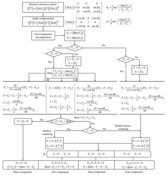
Figure 1.
Flowchart of the decomposition method.
4. Experimental Results
In this segment, discussions and analyses are presented for five distinct study sites that vary significantly in their temporal attributes, geographical locations, frequency bands, and the distribution patterns captured by various satellite imaging systems, including GF-3, Radarsat-2, and ESAR. The objective is to delve deeper into the unique characteristics of these sites and their corresponding imaging data.
4.1. GF-3 Data Collected over San Francisco, USA
To evaluate the performance of the novel decomposition approach, we initially used San Francisco, USA, as the study site. This area comprises diverse terrains, including oceans, forested regions, and buildings with varying orientations. The azimuth and range resolutions of the GF-3 imagery are set to 8 m × 8 m for enhanced precision. Additionally, to attenuate the speckle noise, a refined Lee filter with a 7 × 7 sliding window is utilized. Figure 2 depicts both a visual image and the corresponding Pauli pseudo-color representation of the selected study area.
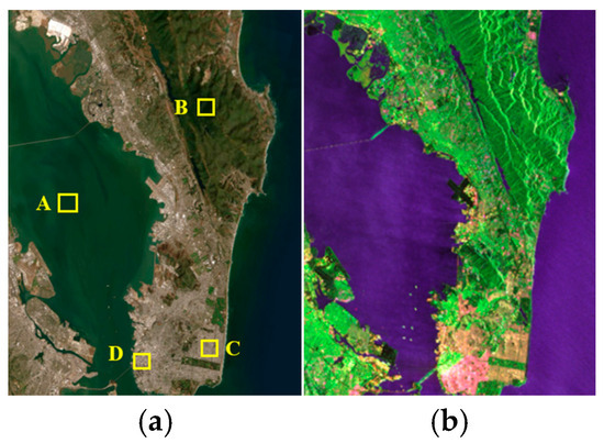
Figure 2.
Acquired GF-3 data in San Francisco, USA. (a) An optical imagery captured by Google Earth, offering a visual representation of the cityscape. Four patches are selected for subsequent analyses (A: ocean; B: forest; C: orthogonal buildings; D: oriented buildings). (b) A complementary Pauli pseudo-color image, which serves as a color-coded visualization of the GF-3 data (red: The term, green: The term, and blue: The term).
To rigorously assess the effectiveness of the proposed approach, we have undertaken a comparative analysis with the decomposition outcomes achieved by employing various techniques such as FDD, Y4R, G4U, AG4U and G5U. To ensure objectivity and eliminate the impact of subjective biases, all methodologies have undergone a standardized preprocessing protocol. The results of these diverse decomposition methods are depicted in Figure 3.
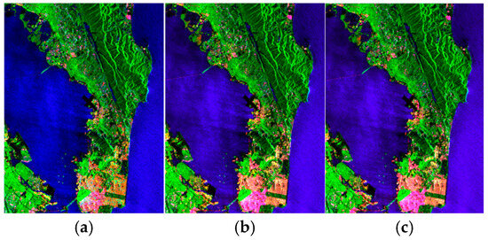
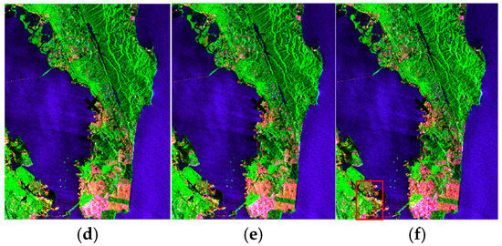
Figure 3.
Scattering power decomposition RGB images using (a) FDD, (b) Y4R, (c) G4U, (d) AG4U, (e) G5U and (f) ExG5U (red: Urban scattering, green: Volume scattering, and blue: Surface scattering).
In Figure 3, the brightness of the colors represents the intensity, where the , half of (in G5U), half of (in G5U and ExG5U), and half of are rendered green; the , half of (in G5U) and half of (in G5U and ExG5U),´ are rendered blue; and the and half of are rendered red, and the decomposition results of the RGB image consists of these three layers. Vegetation areas are predominantly influenced by volume scattering power, while the ocean’s dominant scattering mechanism is surface scattering. Upon comparing the ExG5U method with existing decomposition techniques in Figure 3, it becomes apparent that the ExG5U decomposition method effectively captures the scattering patterns of both aligned and perpendicular building areas, significantly contributing to a notable reduction in volume scattering.
To quantitatively assess the efficacy of the ExG5U approach, four patches have been chosen: A for ocean, B for forest, C for orthogonally aligned buildings, and D for oriented buildings, as depicted in Figure 2a. Patches A and B are used to demonstrate the validation of the proposed method, while patches C and D are selected to analyze the performance of the proposed method in building areas. Figure 4 showcases the average power metrics for these selected patches, encompassing results from six decomposition techniques: FDD, Y4R, G4U, AG4U, G5U and ExG5U.
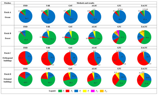
Figure 4.
The mean power statistics of the selected patches depicted in Figure 2a, encompassing the approaches FDD, Y4R, G4U, AG4U, G5U and ExG5U.
In patches A and B, specific interpretations are offered for the dominant scattering mechanisms observed in ocean and vegetation regions. For the ocean areas, surface scattering emerges as the predominant scattering process, with respective percentages of 84.3%, 85%, 85.2%, 85.4%, 86.1% and 87.4% for FDD, Y4R, G4U, AG4U, G5U and ExG5U. Each of these six techniques effectively captures the scattering characteristics of the ocean environment. On the contrary, in vegetated regions, volume scattering assumes a dominant role, with varying percentages of 87.5% to 44.7% across the same methods. Worth mentioning is that for specific techniques like G5U and ExG5U, the composite scattering power components ( and ) are determined, considering the volume scattering component in both and generated compounds. This comprehensive analysis validates the capability of these decomposition methods to offer sound insights into the scattering mechanisms within both vegetated and ocean landscapes.
In the patch designated C within the orthogonal building zone, a consistent scattering phenomenon emerges as the dominant mechanism—double-bounce scattering. This pattern aligns with previous decomposition techniques, indicating its prevalence in such environments. Specifically, the contribution of double-bounce scattering power in patch C stands prominent, accounting for 56.5% for FDD, 56.8% for Y4R, 57% for G4U, 57.1% for AG4U, 58.7% for G5U, and 59.2% for ExG5U. Notably, the percentages of other scattering components like and are negligible due to the minimal contribution of cross-pol power from the orthogonal structure.
Within the building area known as patch D, structures exhibit a nearly 45-degree angle to the radar line of sight. However, traditional decomposition methods tend to misinterpret the dominant scattering mechanism of buildings with such prominent orientation angles, incorrectly labeling it as volume scattering. This often leads to the occurrence of OVS. Interestingly, Figure 4 illustrates how decomposition techniques like G5U can significantly minimize the contributions of volume scattering power. Even more impressively, the application of ExG5U provides further mitigation of OVS. Specifically, for the oriented building area, ExG5U manages to drastically lower the volume scattering component from 68.5% (as initially indicated by FDD) to a mere 31.8%. Furthermore, the proportion of double-bounce scattering undergoes a notable increase, rising from 17.2% with FDD to 30.6% with ExG5U. This demonstrates the remarkable ability of ExG5U to accurately discern and characterize the scattering mechanisms within oriented buildings.
When dealing with the challenge of interpreting scattering mechanisms in patches C and D, which are characterized by buildings with diverse orientation angles, the proposed method notably diminishes the percentage of volume scattering. This reduction in volume scattering power is then redistributed to surface scattering and double-bounce/oriented dihedral scattering mechanisms. The method introduced in this paper efficiently tackles oriented building areas through the adaptive utilization of refined volume scattering models. The resulting decompositions accurately reflect the terrain types, surpassing the limitations of prior methods and providing a more accurate understanding of the scattering phenomena in these complex environments.
In order to better analyze the effectiveness of the method in the area of buildings with complex orientation angles, the red rectangular region in Figure 3f is selected as the study area. The dominant feature types in this region are buildings with various orientation angles and the heights of the buildings are relatively similar. The mean power statistics for the decompositions results obtained via the aforementioned six methods are listed in Table 1. In Table 1, double-bounce scattering and surface scattering obtained from the decoding of the ExG5U method are significantly higher than the other methods. Compared with the other five methods, the decomposition results are more consistent with the ground truth and can be used to better describe the scattering mechanisms in complex orientation building regions, which can effectively alleviate the OVS problem.

Table 1.
Mean power statistics of the selected patch in Figure 3f (%).
For the model-based decomposition method, the occurrence of negative scattering powers is an important indicator to evaluate the performance of the method. Negative scattering powers typically occur in surface scattering or double-bounce scattering because of the prioritized calculation of the volume, wire, oriented dipole and compound dipole scattering components. The percentages of the negative scattering powers obtained via the aforementioned six decomposition methods (FDD, Y4R, G4U, AG4U, G5U and ExG5U) are listed in Table 2. In Table 2, compared with the five existing decomposition methods, the number of negative scattering power pixels is reduced by using the ExG5U, which has the potential to reduce the negative power pixel amount.
Table 2.
Percentage of pixels with negative scattering powers.
4.2. Urban High-Density Building Research Area
Utilizing a GF-3 satellite image captured in Guizhou Province, China, which boasts a resolution of 8 m in both the azimuth and range directions, we conduct a thorough evaluation of the credibility of the proposed methodology. This particular image offers a comprehensive view of the diverse terrain types present in the region, encompassing a wide array of orthogonal buildings, precisely oriented structures, intricate road networks, and dense vegetation areas. Figure 5 showcases both the optical image and its corresponding Pauli pseudo color map, providing a visual representation of the terrain’s intricate details and features.
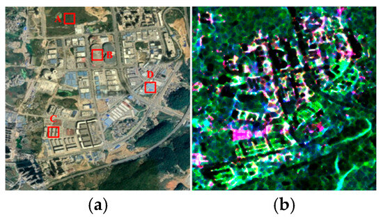
Figure 5.
C-band GF-3 satellite imagery in Guizhou, China: (a) Google Earth’s optical viewpoint and (b) its complementary Pauli pseudo-color representation (red: The term, green: The term, and blue: The term). Patches A–D are the selected study sites for performance comparison and analysis of decomposition methods.
Figure 6 showcases a diverse collection of decomposed images resulting from the aforementioned decomposition techniques. A thorough examination reveals that the double-bounce scattering effect is particularly prominent in orthogonally aligned buildings, whereas it diminishes in structures with larger orientation angles. A comparative analysis of Figure 6c–f with Figure 6a,b highlights the substantial impact of enhancing scattering power components and integrating phase compensation procedures. As a result, areas occupied by buildings are now depicted in shades of red or VioletRed, significantly improving the interpretability of scattering patterns and enhancing the visualization of image details. Notably, Figure 6f stands out in its ability to discern scattering mechanisms within buildings that vary in orientation angles. The proposed approach emerges as an advanced decomposition methodology, adeptly distinguishing the corresponding scattering mechanisms among diverse terrain features.
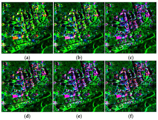
Figure 6.
Decomposition results obtained via (a) FDD, (b) Y4R, (c) G4U, (d) AG4U, (e) G5U and (f) ExG5U (red: Urban scattering, green: Volume scattering, and blue: Surface scattering).
To assess the efficacy of the ExG5U approach, we selectively targeted four regions (highlighted by red rectangles in Figure 5a) for quantitative comparative analysis. We calculated the contributions of surface, double-bounce, volume, and additional scattering mechanisms (, , ) and depicted the respective percentages in Figure 7. In this figure, all the mentioned decomposition methods accurately decipher the dominant scattering mechanisms associated with the selected forests, bare ground, and orthogonally aligned buildings. Notably, the ExG5U method demonstrates superior double-bounce scattering prowess. Specifically, in the area encompassing buildings with significant orientation angles, the double-bounce scattering component increased by 13.9%, 10.5%, 6.7%, 6.3% and 4.5% over FDD, Y4R, G4U, AG4U, and G5U, respectively. Conversely, the volume scattering component declined compared to other methods. These observations align closely with the actual attributes of the study sites. The results further authenticate that the proposed method, leveraging unitary compensation and refined volume scattering models, effectively mitigates the risk of OVS in urban environments. This methodology enables a precise and logical characterization of scattering mechanisms within building areas, particularly those with oriented structures.
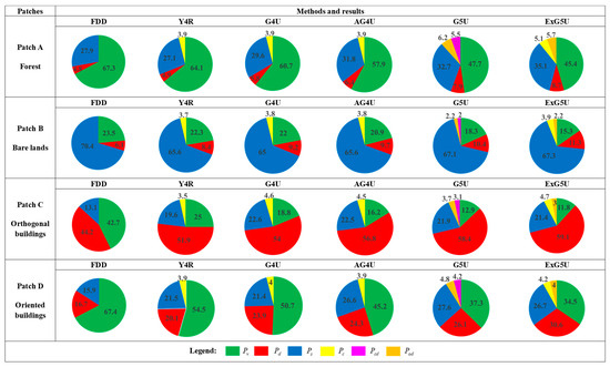
Figure 7.
Mean power statistics for the decompositions results of the selected patches in Figure 5a.
4.3. Research Sites for Distributed Buildings
To demonstrate the robustness of the proposed method, this subsection applies it to an image capturing distributed buildings in Hainan Province, China, which possesses dimensions of 5969 × 4025 pixels. The focal study site encompasses clusters of buildings in Meilan District, Fucheng Town, and adjacent regions, inclusive of Meilan Airport. Figure 8 showcases the optical image along with the Pauli decomposition results, offering valuable insights into the scattering properties of the diverse urban elements within the investigated area.
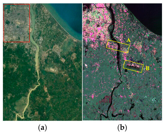
Figure 8.
Detailed examination of C-band data from the GF-3 satellite in Hainan Province, China, with (a) Google Earth optical image and (b) accompanying Pauli pseudo-color mapping (red: The term, green: The term, and blue: The term).
Utilizing the Pauli decomposition findings, the red rectangular indicator in Figure 8a underscores the distinctive double-bounce scattering phenomenon observed in densely populated urban areas. In contrast, areas characterized by sparse buildings surrounded by lush vegetation tend to exhibit OVS due to the dominance of volume scattering over the scattering power of the sparsely distributed buildings.
Figure 9 presents the decomposition results of the aforementioned methods. Specifically, Figure 9f illustrates the ability to discern the scattering mechanisms of both large-scale buildings with orthogonal and directional structures, as well as those buildings interspersed within vegetated areas. The decomposition results for building regions, particularly those with distributed buildings, are obtained, effectively suppressing the occurrence of OVS.
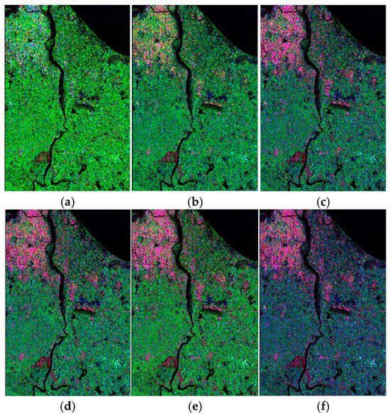
Figure 9.
Decomposition images obtained via (a) FDD, (b) Y4R, (c) G4U, (d) AG4U, (e) G5U and (f) ExG5U (red: Urban scattering, green: Volume scattering, and blue: Surface scattering).
To comprehensively evaluate the performance of our novel method in handling images with distributed buildings, we have specifically chosen two diverse scenarios: airport terminals and dispersed villages, both exhibiting scattered buildings. These areas are prominently marked with yellow rectangles in Figure 8b for a detailed evaluation. As illustrated in Figure 10, the proposed ExG5U method diminishes the influence of volume scattering power while enhancing the contribution of double-bounce scattering power. This allows for a more accurate interpretation of the scattering mechanisms within the building areas. The decomposition results convincingly demonstrate that the scattering characteristics identified by ExG5U closely align with ground truth observations. Therefore, the proposed decomposition technique effectively maintains the textural intricacies of buildings while precisely disentangling the scattering mechanisms associated with diverse terrain types.
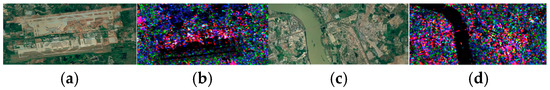
Figure 10.
Results for typical regions. (a,b) Optical images of region A and decomposition results obtained by the proposed method. (c,d) Optical images of region B and decomposition results obtained by the proposed method. Red: Urban scattering, green: Volume scattering, and blue: Surface scattering.
4.4. Radarsat-2 Data Collected over San Francisco, USA
In this subsection, we leverage C-band Radarsat-2 data, encompassing a spatial extent of 14,413 × 2820 pixels, to evaluate the decomposition performance in urban areas and validate the proposed methodology’s effectiveness across similar bands and distinct satellites. This imagery, captured in 2008, boasts a fine spatial resolution of 4.7 m in both range and azimuth directions. For our analysis, we select a window size of 9 × 3. Figure 11 juxtaposes the optical image of the study site with its corresponding Pauli RGB representation, highlighting the similarity in land cover composition to that captured by GF-3. Furthermore, Figure 12 presents pseudo-color maps showcasing the decomposition results derived from six distinct decomposition techniques: FDD, Y4R, G4U, AG4U, G5U and ExG5U. These methods, as earlier described in detail, offer a comprehensive assessment of the urban area decomposition.
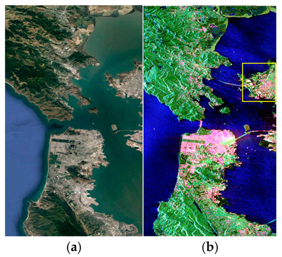
Figure 11.
RADARSAT-2 data collected over San Francisco, USA. (a) Optical image on Google Earth. (b) Corresponding Pauli pseudo-color image (red: The term, green: The term, and blue: The term).
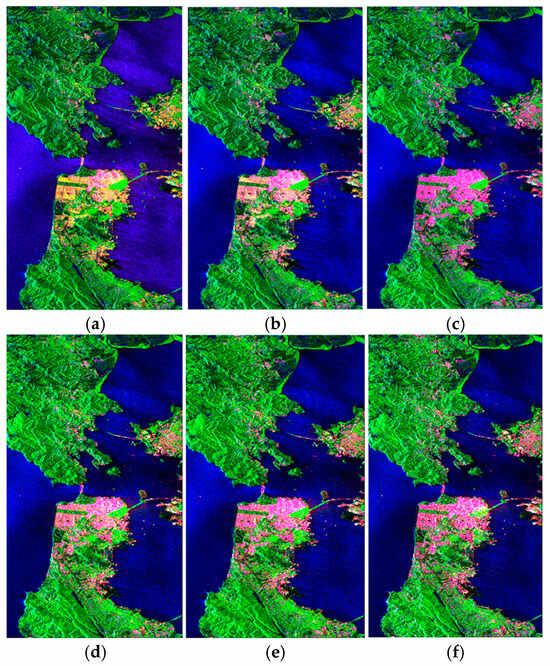
Figure 12.
Decomposition images obtained via (a) FDD, (b) Y4R, (c) G4U, (d) AG4U, (e) G5U and (f) ExG5U (red: Urban scattering, green: Volume scattering, and blue: Surface scattering).
To delve deeper into the performance evaluation of ExG5U specifically in building areas, a representative patch containing buildings with diverse orientation angles has been chosen, visible in Figure 11b. Figure 13 exhibits enlarged decomposition results of the target site, achieved through the aforementioned decomposition techniques, alongside their corresponding optical counterparts.
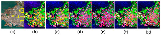
Figure 13.
The images enclosed within the yellow boxed region of Figure 11b are presented as follows: subfigure (a) depicts the optical image of the chosen patch, while subfigures (b–g) exhibit the corresponding decomposition results derived from the FDD, Y4R, G4U, AG4U, G5U and ExG5U methodologies, respectively (red: Urban scattering, green: Volume scattering, and blue: Surface scattering).
Figure 13a depicts a comparative study of two oriented building area patches labeled I and II, alongside an orthogonal building area patch III. As the decomposition method undergoes enhancements, the results obtained via ExG5U progressively align more closely with the actual terrain types. This alignment facilitates a precise understanding of the scattering mechanisms exhibited by various land covers. Additionally, Figure 14 provides further clarity by presenting histograms of orientation angles for these selected patches. By combining the observations from Figure 13 and Figure 14, it becomes evident that all decomposition methods effectively interpret the scattering mechanisms in orthogonal building areas, especially emphasizing the dominance of double-bounce scattering. However, when it comes to oriented building areas, the ExG5U method emerges as the superior choice for interpreting the scattering mechanisms.
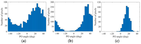
Figure 14.
Histogram representations of selected patches I, II, and III.
To quantitatively assess the proficiency of ExG5U in handling oriented building areas, Figure 15 presents a comparative analysis of the mean power statistics for the specified patches I and II. In patch I, ExG5U exhibits remarkable performance, surpassing FDD, Y4R, G4U, AG4U, and G5U by achieving a significant reduction in volume scattering by 50.5%, 47.4%, 25.1%, 20.6%, and 2.7%, respectively. This notable decrease is accompanied by a concurrent enhancement in double-bounce scattering, which is crucial for accurate interpretation. Similarly, in patch II, ExG5U maintains its superiority, accurately enhancing double-bounce scattering and overcoming the challenges posed by OVS. This consistency in performance demonstrates the effectiveness of ExG5U in interpreting the scattering mechanism in oriented building areas.
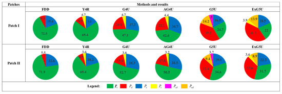
Figure 15.
Illustrating the average power metrics for diverse spectral decomposition techniques, including FDD, Y4R, G4U, AG4U, G5U, and ExG5U, highlighting Patches I and II.
4.5. L-Band ESAR Data
To evaluate the performance of ExG5U in decomposing multi-band SAR imagery, we utilize the L-band ESAR dataset. The target area, located in Oberpfaffenhofen, Germany, spans a 1300 × 1200-pixel region. Owing to the satisfactory number of equivalent looks in the dataset, further averaging or filtering measures are deemed unnecessary. Figure 16 exhibits a visual illustration of the study area, presenting both an optical image and its corresponding Pauli RGB representation for comparative analysis.
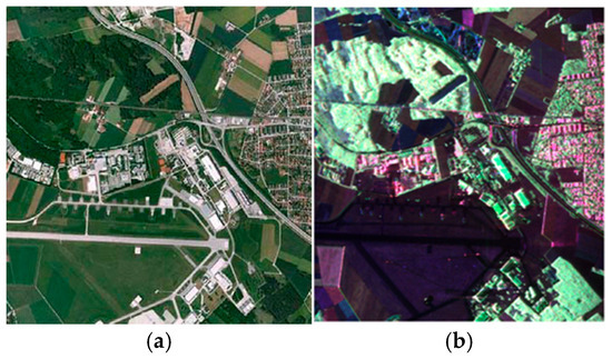
Figure 16.
L-Band ESAR imagery of the Oberpfaffenhofen study area in Germany: (a) Google Earth optical view, (b) Pauli pseudo-color representation (red: The term, green: The term, and blue: The term).
In the preceding sections, a comparative evaluation is undertaken between the ExG5U method and seven existing decomposition approaches. Given that both G5U and ExG5U segment the coherency matrix into five scattering components, this particular segment delves into the nuances between ExG5U and G5U. The intention is to highlight the enhanced performance of the refined volume scattering models utilized in ExG5U. Figure 17b,c presents the decomposition results of ExG5U and G5U, respectively.
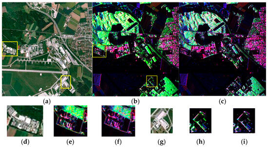
Figure 17.
(a,d,g) are the optical images of entire image and the selected patches. Illustrations of the decomposition results: (b) G5U vs. (c) ExG5U. Specifically, (e,h) highlight G5U results for the selected patches, while (f,i) showcase the ExG5U outputs for the selected patches. Red: Urban scattering, green: Volume scattering, and blue: Surface scattering.
As visualized in Figure 17a–c, regions of buildings that are aligned or near-aligned with the flight trajectory exhibit similar decomposition results when utilizing G5U and ExG5U. This resemblance suggests that both techniques effectively capture the scattering behaviors within these building zones. To gain a deeper understanding of the performance of G5U and ExG5U, we have selected two specific oriented building regions depicted in Figure 17a for a comprehensive analysis. Figure 17e,f,h,i offers magnified views of the optical images and decomposition results pertaining to these regions.
Upon a thorough comparison of the decomposition outcomes with the optical imagery depicted in Figure 16a, a conspicuous observation emerges: ExG5U offers a more intuitive visualization of the scattering dynamics within the oriented building regions compared to G5U. Notably, the building area is decomposed into distinct red/pink components by ExG5U, providing a clearer insight into the underlying scattering processes.
To further substantiate the rationality of the decomposition results in the targeted regions, we apply the unsupervised Wishart classification methodology proposed in [28] to both G5U and ExG5U decompositions. Figure 18b,c showcases the classification results achieved by each technique, while Figure 18e,f,h,i provides magnified views of specific zones. According to these classification results, ExG5U significantly mitigates the impact of volume scattering and addresses the issue of OVS. Consequently, the dominant scattering mechanism in urban areas with significant orientation angles transitions to double-bounce scattering, aligning with ground-based observations.
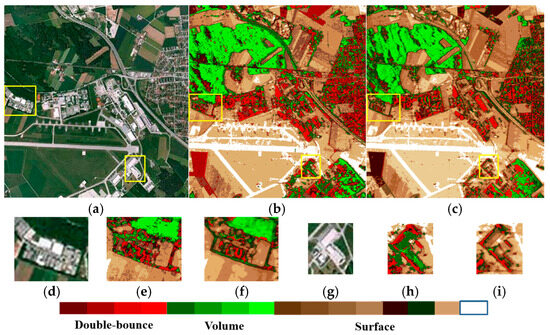
Figure 18.
(a,d,g) are the optical images of entire image and the selected patches. The comprehensive analysis: classification results derived from (b) G5U and (c) ExG5U decompositions. Specifically, (e,h) are G5U-based classification results, and (f,i) are ExG5U-based classification results.
In summary, the five-component decomposition approach, which utilizes refined volume scattering models and HAC, emerges as a highly efficacious method for analyzing the scattering mechanisms of diverse land cover types. There is one aspect that requires caution when interpreting the results of the proposed method. The method proposed in this paper mitigates the OVS problem well by using refined volume scattering models and angle compensations, and the scattering mechanism in some of the oriented building regions is well interpreted. However, there are still some large oriented building regions whose scattering mechanisms cannot be deciphered accurately. How to further eliminate the OVS problem of these building regions perfectly is still the focus of subsequent research, and the method proposed in this paper can be used as the basic method in subsequent research.
5. Conclusions
Urban areas, characterized by their intricate landscape and heterogeneous feature distribution, present formidable obstacles in analyzing polarimetric scattering patterns. These complexities often lead to interpretive challenges, such as confusing dihedral scattering from buildings facing the radar line of sight with volume scattering. The similarity in polarization signatures creates confusion in distinguishing building areas from vegetated regions. In this paper, we introduce an enhanced hierarchical approach called ExG5U to tackle this challenge. The method incorporates unitary compensation and urban-specific refined volume scattering models. Through this integration, ExG5U effectively identifies ambiguous areas and circumvents the difficulties posed by oriented volume scattering. To further strengthen the adaptability of the proposed method, we have reformulated the branch conditions for selecting the refined volume scattering models. This ensures that the volume scattering model of each pixel is specifically designed to fit its unique terrain type. To validate the effectiveness of this approach, we have selected three GF-3 datasets, each exhibiting distinct temporal, geographical, and structural attributes. These datasets encompass multiple urban areas with varying orientations, enabling us to compare the proposed method with a range of decomposition techniques. Additionally, we have applied the proposed method to Radarsat-2 data and ESAR data to assess its robustness across different satellite systems and frequency bands. The results show that the proposed ExG5U method achieves better results in overcoming OVS in building regions, especially in oriented building regions, and can serve as an important complement to polarimetric decomposition methods, providing valuable insights for further achieving fine decoding of building scattering mechanisms.
Author Contributions
Conceptualization, Y.W. and W.Y.; methodology, Y.W. and C.W.; software, Y.W. and B.L.; validation, Y.W. and D.G.; investigation, D.G.; writing—original draft preparation, Y.W. and D.G.; writing—review and editing, Y.W., D.G., B.L., W.Y. and C.W.; funding acquisition, D.G. All authors have read and agreed to the published version of the manuscript.
Funding
This work was supported by the National Key Research and Development Program of China under grant 2021YFC3000400.
Data Availability Statement
Data will be made available on request.
Conflicts of Interest
The authors declare no conflicts of interest.
References
- Xiang, D.; Tang, T.; Ban, Y.; Su, Y.; Kuang, G. Unsupervised Polarimetric SAR Urban Area Classification Based on Model-Based Decomposition with cross scattering. ISPRS J. Photogramm. Remote Sens. 2016, 116, 86–100. [Google Scholar] [CrossRef]
- Xi, Y.; Lang, H.; Tao, Y.; Huang, L.; Pei, Z. Four-Component Model-Based Decomposition for Ship Targets Using PolSAR Data. Remote Sens. 2016, 9, 621–638. [Google Scholar] [CrossRef]
- Zhu, Y.; Ai, J.; Wu, L.; Guo, D.; Jia, W.; Hong, R. An Active Multi-Target Domain Adaptation Strategy: Progressive Class Prototype Rectification. IEEE Trans. Multimed. 2025, 27, 1874–1886. [Google Scholar] [CrossRef]
- Wang, Y.; Yu, W.; Wang, R.; Wang, L.; Ge, D.; Liu, X.; Wang, C.; Liu, B. An Improved Urban Area Extraction Method for PolSAR Data Using Eigenvalues and Optimal Roll-Invariant Features. IEEE J. Sel. Top. Appl. Earth Observ. Remote Sens. 2024, 17, 6455–6467. [Google Scholar] [CrossRef]
- Anconitano, G.; Lavalle, M.; Acuna, M.A.; Pierdicca, N. Sensitivity of Polarimetric SAR Decompositions to Soil Moisture and Vegetation Over Three Agricultural Sites Across a Latitudinal Gradient. IEEE J. Sel. Top. Appl. Earth Observ. Remote Sens. 2024, 17, 3615–3634. [Google Scholar] [CrossRef]
- Lee, J.; Pottier, E. Polarimetric Radar Imaging: From Basics to Applications; CRC Press: Boca Raton, FL, USA, 2009; pp. 3–9. [Google Scholar]
- Cloude, S.R.; Pottier, E. A Review of Target Decomposition Theorems in Radar Polarimetry. IEEE Trans. Geosci. Remote Sens. 1996, 34, 498–518. [Google Scholar] [CrossRef]
- Freeman, A.; Durden, S.L. A Three-Component Scattering Model for Polarimetric SAR Data. IEEE Trans. Geosci. Remote Sens. 1998, 36, 963–973. [Google Scholar] [CrossRef]
- Yamaguchi, Y.; Moriyama, T.; Ishido, M.; Yamada, H. Four-Component Scattering Model for Polarimetric SAR Image Decomposition. IEEE Trans. Geosci. Remote Sens. 2005, 43, 1699–1706. [Google Scholar] [CrossRef]
- Zhang, L.; Zou, B.; Zhang, Y. Multiple-Component Scattering Model for Polarimetric SAR Image Decomposition. IEEE Geosci. Remote Sens. Lett. 2008, 5, 603–607. [Google Scholar] [CrossRef]
- Xiang, D.; Ban, Y.; Su, Y. Model-Based Decomposition with Cross Scattering for Polarimetric SAR Urban Areas. IEEE Geosci. Remote Sens. Lett. 2015, 12, 2496–2500. [Google Scholar] [CrossRef]
- Singh, G.; Yamaguchi, Y. Model-Based Six-Component Scattering Matrix Power Decomposition. IEEE Trans. Geosci. Remote Sens. 2018, 56, 5687–5704. [Google Scholar] [CrossRef]
- Singh, G.; Malik, R.; Mohanty, S.; Rathore, V.S.; Yamada, K.; Umemura, M.; Yamaguchi, Y. Seven-Component Scattering Power Decomposition of PolSAR Coherency Matrix. IEEE Trans. Geosci. Remote Sens. 2019, 57, 8371–8382. [Google Scholar] [CrossRef]
- Yamaguchi, Y.; Sato, A.; Boerner, W.M.; Sato, R.; Yamada, H. Four-Component Scattering Power Decomposition with Rotation of Coherency Matrix. IEEE Trans. Geosci. Remote Sens. 2011, 49, 2251–2258. [Google Scholar] [CrossRef]
- Li, H.; Chen, J.; Li, Q.; Wu, G.; Chen, J. Mitigation of Reflection Symmetry Assumption and Negative Power Problems for the Model-Based Decomposition. IEEE Trans. Geosci. Remote Sens. 2016, 54, 7261–7271. [Google Scholar] [CrossRef]
- Yamada, H.; Suzuki, Y.; Kawada, M.; Sato, R. Five-Component Scattering Power Decomposition of PolSAR Data Without Polarization Rotation. In Proceedings of the IGARSS 2023—2023 IEEE International Geoscience and Remote Sensing Symposium, Pasadena, CA, USA, 16–21 July 2023; pp. 1614–1617. [Google Scholar]
- Malik, R.; Singh, G.; Dikshit, O.; Yamaguchi, Y. Model-Based Nine-Component Scattering Matrix Power Decomposition. IEEE Geosci. Remote Sens. Lett. 2024, 21, 1–5. [Google Scholar] [CrossRef]
- Singh, G.; Yamaguchi, Y.; Park, S.E. General Four-Component Scattering Power Decomposition with Unitary Transformation of Coherency Matrix. IEEE Trans. Geosci. Remote Sens. 2013, 51, 3014–3022. [Google Scholar] [CrossRef]
- Bhattacharya, A.; Singh, G.; Manickam, S.; Yamaguchi, Y. An Adaptive General Four-Component Scattering Power Decomposition with Unitary Transformation of Coherency Matrix (AG4U). IEEE Geosci. Remote Sens. Lett. 2015, 12, 2110–2114. [Google Scholar] [CrossRef]
- Quan, S.; Xiang, D.; Xiong, B.; Canbin, H.; Gangyao, K. A Hierarchical Extension of General Four-Component Scattering Power Decomposition. Remote Sens. 2017, 9, 856. [Google Scholar] [CrossRef]
- Wang, Y.; Yu, W.; Liu, X.; Wang, C.; Kuijper, A.; Guthe, S. Demonstration and Analysis of an Extended Adaptive General Four-Component Decomposition. IEEE J. Sel. Top. Appl. Earth Obs. Remote Sens. 2020, 13, 2573–2586. [Google Scholar] [CrossRef]
- Malik, R.; Singh, G.; Dikshit, O.; Yamaguchi, Y. General Five-Component Scattering Power Decomposition with Unitary Transformation (G5U) of Coherency Matrix. Remote Sens. 2023, 15, 1332. [Google Scholar] [CrossRef]
- Sato, A.; Yamaguchi, Y.; Singh, G.; Park, S. Four-Component Scattering Power Decomposition with Extended Volume Scattering Model. IEEE Geosci. Remote Sens. Lett. 2012, 9, 166–170. [Google Scholar] [CrossRef]
- Antropov, O.; Rauste, Y.; Hame, T. Volume Scattering Modeling in PolSAR Decompositions: Study of Alos PolSAR Data over Boreal Forest. IEEE Trans. Geosci. Remote Sens. 2011, 49, 3838–3848. [Google Scholar] [CrossRef]
- Wang, Y.; Yu, W.; Wang, C.; Liu, X. A Modified Four-Component Decomposition Method with Refined Volume Scattering Models. IEEE J. Sel. Top. Appl. Earth Obs. Remote Sens. 2020, 13, 1946–1958. [Google Scholar] [CrossRef]
- Wang, Y.; Yu, W.; Liu, X.; Wang, C. Seven-Component Decomposition Using Refined Volume Scattering Models and New Configurations of Mixed Dipoles. IEEE J. Sel. Top. Appl. Earth Obs. Remote Sens. 2020, 13, 4339–4351. [Google Scholar] [CrossRef]
- Chen, Y.; Zhang, L.; Mallorqui, J.J.; Zou, B. Modified Oriented Dihedral Model for Scattering Characteristic Description with PolSAR Data. IEEE J. Sel. Top. Appl. Earth Obs. Remote Sens. 2024, 17, 4829–4844. [Google Scholar] [CrossRef]
- Lee, J.S.; Grunes, M.R.; Pottier, E.; Ferro-Famil, L. Unsupervised Terrain Classification Preserving Polarimetric Scattering Characteristics. IEEE Trans. Geosci. Remote Sens. 2004, 42, 722–731. [Google Scholar]
Disclaimer/Publisher’s Note: The statements, opinions and data contained in all publications are solely those of the individual author(s) and contributor(s) and not of MDPI and/or the editor(s). MDPI and/or the editor(s) disclaim responsibility for any injury to people or property resulting from any ideas, methods, instructions or products referred to in the content. |
© 2025 by the authors. Licensee MDPI, Basel, Switzerland. This article is an open access article distributed under the terms and conditions of the Creative Commons Attribution (CC BY) license (https://creativecommons.org/licenses/by/4.0/).