Snow Depth Retrieval Using Sentinel-1 Radar Data: A Comparative Analysis of Random Forest and Support Vector Machine Models with Simulated Annealing Optimization

Abstract

Snow plays a crucial role in global climate regulation, hydrological processes, and environmental change, making the accurate acquisition of snow depth data highly significant. In this study, we used Sentinel-1 radar data and employed a simulated annealing algorithm to select the optimal influencing factors from radar backscatter characteristics and spatiotemporal geographical parameters within the study area. Snow depth retrieval was subsequently performed using both random forest (RF) and Support Vector Machine (SVM) models. The retrieval results were validated against in situ measurements and compared with the long-term daily snow depth dataset of China for the period 2017–2019. The results indicate that the RF model achieves better agreement with the measured data than existing snow depth products. Specifically, in the Xinjiang region, the RF model demonstrates superior performance, with an R² of 0.92, a root mean square error (RMSE) of 2.61 cm, and a mean absolute error (MAE) of 1.42 cm. In contrast, the SVM regression model shows weaker agreement with the observations, with an R² lower than that of the existing snow depth product (0.51) in Xinjiang, and it performs poorly in other regions as well. Overall, the SVM model exhibits deficiencies in both predictive accuracy and spatial stability. This study provides a valuable reference for snow depth retrieval research based on active microwave remote sensing techniques.

1. Introduction

Snow is a major component of the cryosphere and exhibits high sensitivity to climate, hydrological processes, and environmental changes, providing critical feedback information [1]. With global climate warming, the dynamic variations in snow have become one of the key factors influencing socioeconomic development and natural ecosystems [2,3]. As one of the primary attributes of snow cover, snow depth is a crucial parameter for studying global energy balance, land–atmosphere interactions, and ecological models development [4,5,6,7]. Therefore, accurate snow depth data are of great importance for understanding the water cycle, climate change, and ecosystem dynamics [8].

At present, snow depth data are primarily obtained through ground-based station observations and satellite remote sensing. Compared with other snow depth products, ground observation data offer higher accuracy and have been widely used by researchers to study the spatial distribution characteristics of parameters such as snow water equivalent, snow depth in snow-covered regions, and changes in snow resources. However, due to the influence of complex terrain, snow depth observation stations are often unevenly distributed and have limited spatial coverage, making it difficult to meet the requirements for large-scale snow monitoring [9,10]. In recent years, with the advancement of computer vision technologies, ground-based camera monitoring and UAV LiDAR measurements have emerged as novel technical approaches for snow depth estimation at local scales. Tanis et al. demonstrated synergistic monitoring using webcams and ultrasonic sensors, where camera data (72–94% accuracy) effectively compensated for ultrasonic measurement limitations when snow depth was below 2 cm [11]. Jenssen et al. developed a UAV-mounted ultra-wideband radar system for snow detection, with tests showing strong correlation (R = 0.87) with field measurements, along with enhanced anti-interference capability, significantly improving detection efficiency and operational safety [12].

Satellite remote sensing has led to the development of various retrieval algorithms, including statistical inversion methods, physical models, and machine learning approaches. Statistical inversion methods are based on empirical relationships between satellite-observed microwave brightness temperature data and snow depth. The widely applied NASA algorithm employed a linear regression model using the brightness temperature difference at 18 GHz and 37 GHz with horizontal polarization for snow depth retrieval. Gao et al. [13] improved the NASA snow depth algorithm and used SSM/I data for real-time snow depth monitoring on the Tibetan Plateau. Jiang et al. [14] developed an operational snow monitoring algorithm for China by integrating multi-source remote sensing data (AMSR-E/FY3B-MWRI brightness temperature) with ground observations through a land cover type-weighted snow depth retrieval approach. Gao et al. [15] employed Level-1 brightness temperature data from FY-3B/MWRI and developed a new semi-empirical algorithm to retrieve snow depth over the Tibetan Plateau. Comparisons with AMSR2 snow depth products showed that this method demonstrated better applicability to the Tibetan Plateau than global snow depth algorithms. This approach is conceptually simple, requires fewer input parameters, and allows for real-time and efficient processing of satellite data for snow depth retrieval [16,17]. However, uncertainties still exist due to the influence of factors such as spatial resolution, snow surface heterogeneity, and atmospheric conditions during the acquisition of brightness temperature data and snow depth products [18,19].

Physical inversion methods primarily retrieve snow depth based on the physical properties of snow and the propagation characteristics of microwaves through the snowpack. Many researchers have investigated the relationships between the microwave radiative properties of snow and factors such as snow depth and snow density, resulting in the development of various snow microwave radiative transfer models [20,21]. Che et al. [22] developed a physics-based snow depth retrieval method for forested Northeast China using MEMLS, optimizing forest transmissivity via iterative inversion and snow properties through dynamic LUTs. Deng et al. significantly improved the simulation accuracy of snow parameters (SCE/SD/SMR) in alpine regions by assimilating MODIS snow cover data into the FSM2 physical snow model, thereby validating the effectiveness of integrated physical modeling and remote sensing retrieval approaches [23]. Physical models are widely studied due to their solid theoretical foundation. However, they involve complex processes during snow depth retrieval, require high model precision, and depend on numerous input parameters—many of which are difficult to obtain from ground measurements. Consequently, the application of physical models remains significantly limited [18,24].

Machine learning algorithms have been widely applied in recent years to snow depth retrieval, as they effectively address the nonlinear relationships between microwave brightness temperature and snowpack parameters and are capable of modeling complex many-to-many functional relationships. Yao et al. [25] proposed a novel retrieval algorithm based on deep convolutional neural networks, which enables the extraction of snow layer thickness and temperature with higher prediction accuracy. Wei et al. [26] employed machine learning techniques to capture the nonlinear relationship between snow depth and snow characteristics, developing a retrieval algorithm with significant improvements in spatial resolution and retrieval accuracy. Li et al. [27] utilized an artificial neural network (ANN) approach to reconstruct historical snow depth from 1901 to 1960 in the Tianshan region of China, analyzing temporal and spatial variations to provide valuable insights into regional climate change. Xiao et al. [28] proposed a snow depth retrieval method based on support vector regression (SVR), which integrated remote sensing data and terrain parameters to improve accuracy and reduce uncertainty. Yang et al. [29] adopted a random forest (RF) machine learning model for snow depth estimation and found that the RF model performed better on a temporal scale than on a spatial scale, offering an accurate tool for analyzing long-term snow depth changes. Benefiting from their strong function-fitting capabilities, machine-learning methods achieve higher retrieval accuracy and effectively handle the complexity and variability of the snow depth retrieval process. By learning from large-scale datasets and recognizing patterns, they enhance predictive accuracy and enable rapid, real-time computation.

Passive microwave remote sensing can penetrate the snow surface and acquire information about the snowpack interior, making it widely used in snow parameter studies and long-term snow monitoring. However, existing passive microwave remote sensing images have relatively low spatial resolution, which limits their application in high-resolution and high-precision snow parameter research. Compared with optical and passive microwave remote sensing, active microwave remote sensing offers all-weather, day-and-night observation capabilities, unaffected by clouds and precipitation, and can effectively penetrate the snow surface. In recent years, this technology has gradually been applied in the field of snow parameter studies [30]. Yu et al. [31] employed differential coherence from Sentinel-1 SAR imagery to characterize surface disturbances caused by winter storms in Texas and quantified snow depth across the state using machine learning algorithms. Yang et al. [32] improved the SWE retrieval model by using C-band SAR data from the GaoFen-3 (GF-3) satellite combined with land cover classification and polarization decomposition methods, significantly enhancing retrieval accuracy and providing a new technical approach for all-weather, high-resolution regional SWE monitoring.

This study utilized high spatial resolution data obtained from active microwave remote sensing technology, calculating surface information based on the surface backscattering coefficient [33,34], while incorporating geographical and spatiotemporal parameters. First, a simulated annealing algorithm was employed to select the optimal influencing factors from snow radar characteristic parameters and geographic features within the study area. Subsequently, random forest and support vector regression models were applied for snow depth retrieval. The retrieved snow depth results were then validated against the long-term snow depth dataset for China as well as in situ measurement data. Finally, a comparative analysis of the retrieval performance of the two models across different regions was conducted. By leveraging machine learning methods, this study reduced the complexity and variability inherent in snow depth retrieval processes and achieved high-precision snow depth estimation, aiming to provide a valuable reference for snow depth retrieval research based on active microwave remote sensing technology.

2. Materials and Methods

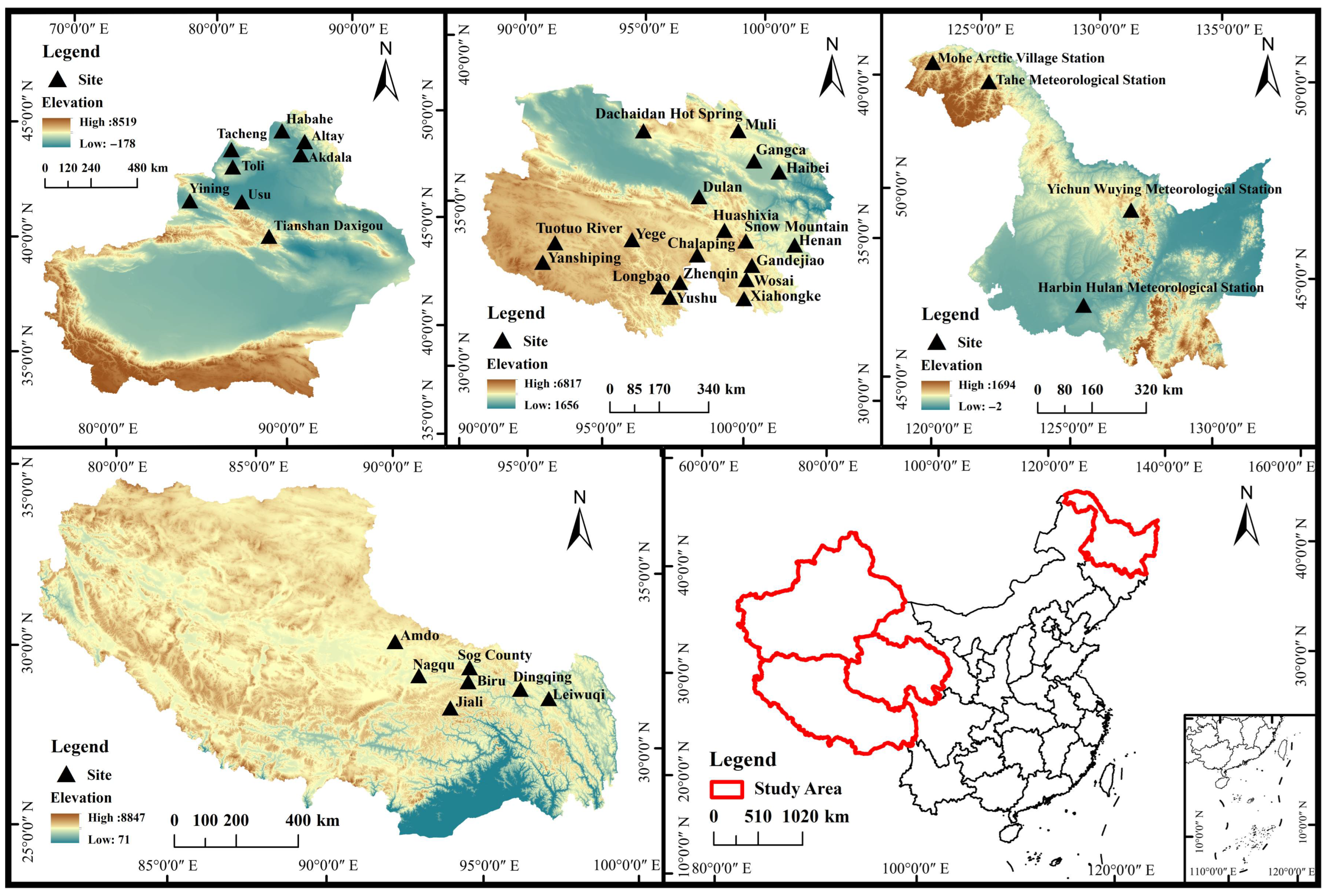
2.1. Data Source

2.1.1. Radar Data

The primary data utilized in this study consisted of radar backscatter characteristics and geospatial-temporal features, all acquired through the Google Earth Engine platform [35]. The radar remote sensing data were derived from Sentinel-1 synthetic aperture radar (SAR) imagery released by the European Space Agency (ESA). Sentinel-1 consists of two satellites, Sentinel-1A and Sentinel-1B, equipped with C-band radar sensors operating at a frequency of 5.405 GHz. These sensors provide all-weather, day-and-night imaging capabilities, widely applied in monitoring surface dynamics, snow and cryosphere research, polar ice observation, and water resource management. Sentinel-1 offers four imaging modes: Interferometric Wide (IW), Extra Wide (EW), Wave (WV), and Stripmap (SM). The IW mode was employed in this study. The utilized data are Ground Range Detected (GRD) products, which have undergone preprocessing steps including thermal noise removal, radiometric calibration, and terrain correction. The dataset contains dual polarization channels, VV and VH, as well as corresponding incidence angle information. The data cover over 30 typical snow monitoring stations across Xinjiang, Qinghai, Tibet, and Heilongjiang, spanning from 1 May 2017 to 1 June 2019. The final Sentinel-1 time series dataset includes VV/VH backscatter intensities and incidence angle information for each station [36]. Additionally, to extract regional geographic environmental features, the study acquired global Shuttle Radar Topography Mission (SRTM) digital elevation model (DEM) data at 30-m resolution [37].

2.1.2. In Situ Measurement Data

The in situ measured snow depth data used in this study were sourced from the China Typical Snow Region Ordinary Station Snow Depth Dataset (2017–2019), a subset of the China Snow Ground Survey Dataset provided by the Northwest Institute of Eco-Environment and Resources, Chinese Academy of Sciences [38]. This dataset includes manual and automatic instrument observations from 41 ordinary meteorological stations located in typical snow-covered regions of China during two snow seasons from 2017 to 2019. The stations were mainly distributed across Xinjiang, Qinghai, Tibet, Inner Mongolia, and Heilongjiang shown in Figure 1. Among these, the ordinary stations in Xinjiang, Qinghai, Inner Mongolia, and Heilongjiang provided snow depth and air temperature data, while those in Tibet recorded snow depth and snow pressure data. The station information for these four regions were summarized in Appendix A.

Due to the limited penetration capability of microwave signals through wet snow, this study focused exclusively on snow depth retrieval during dry snow periods. During the two snow seasons, over 95% of the snow depth observations at the Bange and Dangxiong stations in Tibet recorded 0 cm. In addition, the Nielamu and Cuona stations had relatively limited data samples. Therefore, data from these four stations were excluded from the analysis, and snow depth data from the remaining 37 stations were used. Daily automatic observations from the two snow seasons were selected as the in situ measurement data. Due to equipment limitations and weather-related factors, the quantity of observational data varied across regions. During data preprocessing, anomalous values (−6999) and missing values were removed.

2.1.3. Snow Depth Products

The snow depth products compared in this study were derived from the “China Snow Depth Long Time Series Dataset (1979–2024)”, specifically the snow depth data from 2017 to 2019. This dataset was processed by Che et al. [39] using the Chang algorithm that comprehensively accounts for multiple surface factors. The original data were obtained from the National Snow and Ice Data Center (NSIDC), consisting of daily passive microwave brightness temperature observations from SMMR (1979–1987), SSM/I (1987–2007), and SSMI/S (2008–2020), with a uniform spatial resolution of 0.25° (EASE-Grid). The statistically retrieved snow depth distribution provides comprehensive snow cover information across China from 1 January 1979 to the present. For this study, we specifically used the 2017–2019 subset to ensure temporal alignment with our in situ measurement data.

2.2. Research Methods

2.2.1. Feature Data Processing

The radar backscatter signal exhibits a correlation with snow depth. As snow depth increases, the propagation path length of the radar signal through the snow extends, thereby enhancing opportunities for radar signal scattering [40]. The backscatter signal of snow comprises three components: volume scattering from interactions within the snowpack, surface scattering at the snow–ground interface, and ground scattering at the snow–ground interface [41]. The relationship can be expressed as Equation (1).

$${\mathsf{\sigma }}_{\mathrm{total}}^{\mathrm{pq}}={\mathsf{\sigma }}_{\mathrm{vol}}^{\mathrm{pq}}+{\mathsf{\sigma }}_{\mathrm{surf}}^{\mathrm{pq}}+{\mathsf{\sigma }}_{\mathrm{bkg}}^{\mathrm{pq}}$$

(1)

Among them, $\mathrm{pq}$ represents the polarization mode, ${\mathsf{\sigma }}_{\mathrm{total}}^{\mathrm{pq}}$ represents the total backscatter signal of snow, ${\mathsf{\sigma }}_{\mathrm{vol}}^{\mathrm{pq}}$ corresponds to volume scattering signal within the snowpack, ${\mathsf{\sigma }}_{\mathrm{surf}}^{\mathrm{pq}}$ indicates surface scattering at the air-snow interface, and ${\mathsf{\sigma }}_{\mathrm{bkg}}^{\mathrm{pq}}$ signifies ground scattering at the snow–ground interface. As mentioned above, radar backscatter signals contain retrievable snow depth information, forming the physical basis for snow depth inversion using a random forest model. However, topographic variations significantly influence radar backscatter characteristics, with terrain-induced signal variations often exceeding those caused by surface features [42]. To mitigate topographic effects, this study implemented normalized backscatter correction for both VV and VH polarization signals from Sentinel-1. This standardization process enables direct comparison of radar echoes across different terrain conditions while minimizing topographic influences. The transformation equations are presented below (Equations (2) and (3)):

$$\mathsf{\beta }=\mathsf{\sigma }÷\mathrm{s}\mathrm{i}\mathrm{n}\mathsf{\theta }$$

(2)

$$\mathsf{\gamma }=\mathsf{\sigma }÷\mathrm{c}\mathrm{o}\mathrm{s}\mathsf{\theta }$$

(3)

Among them, $\mathsf{\theta }$ represents the radar incidence angle, $\mathsf{\sigma }$ is referenced to the normalized radar backscatter coefficient, quantifying the backscattered power per unit incident power and characterizing the scattering properties of the target surface. $\mathsf{\beta }$ indicates the normalized backscatter coefficient relative to the radar transmission plane, compensating for geometric distortions. $\mathsf{\gamma }$ is referenced to the plane perpendicular to the signal transmission direction, that is, the terrain surface perpendicular to the radar signal plane. It further corrects for the influence of terrain undulations on backscatter, obtaining ${\mathsf{\beta }}_{\mathrm{VH}}$, ${\mathsf{\gamma }}_{\mathrm{VH}}$, ${\mathsf{\beta }}_{\mathrm{VV}}$, and ${\mathsf{\gamma }}_{\mathrm{VV}}$ radar characteristic data. These parameters are widely used in radar remote sensing, especially in complex terrain regions, as they enhance backscatter data interpretability and measurement accuracy. Existing research has established that the polarimetric backscatter ratio (${\mathsf{\sigma }}_{\mathrm{VH}}/{\mathsf{\sigma }}_{\mathrm{VV}}$) correlates with snow depth, and snow depth inversion models have been successfully developed using this relationship [43]. Accordingly, this study selects seven key parameters for the random forest algorithm: ${\mathsf{\sigma }}_{\mathrm{VH}}$, ${\mathsf{\sigma }}_{\mathrm{VV}}$, ${\mathsf{\beta }}_{\mathrm{VH}}$, ${\mathsf{\gamma }}_{\mathrm{VH}}$, ${\mathsf{\beta }}_{\mathrm{VV}}$, ${\mathsf{\gamma }}_{\mathrm{VV}}$, and ${\mathsf{\sigma }}_{\mathrm{VH}}/{\mathsf{\sigma }}_{\mathrm{VV}}$.

Snow depth distribution exhibits strong spatiotemporal dependence on elevation, slope, aspect, surface roughness, wind speed, and wind direction [44,45,46]. Following established methodologies [47], we incorporated four geographic parameters (elevation, surface roughness, slope, and aspect) and temporal variables. DEM data were processed in ArcGIS 10.2 to extract slope and aspect, with surface roughness calculated using Equation (4):

$${\mathrm{G}}_{\mathrm{r}}=1/\mathrm{c}\mathrm{o}\mathrm{s}{\displaystyle \frac{\mathrm{aspect}}{180}}\times \mathsf{\pi }$$

(4)

Among them, ${\mathrm{G}}_{\mathrm{r}}$ represents surface roughness. Through comprehensive analysis and processing, five geographic feature parameters were derived: elevation, surface roughness, slope, aspect, and date. The complete set of feature parameters used in this study is systematically summarized in

Table 1. Snow depth inversion parameters.

Model Parameters	Feature Variables
Radar feature parameters	${\mathsf{\sigma }}_{\mathrm{VV}}$, ${\mathsf{\sigma }}_{\mathrm{VH}}$, ${\mathsf{\gamma }}_{\mathrm{VV}}$, ${\mathsf{\gamma }}_{\mathrm{VH}}$, ${\mathsf{\beta }}_{\mathrm{VV}}$, ${\mathsf{\beta }}_{\mathrm{VH}}$, ${\mathsf{\sigma }}_{\mathrm{VH}}/{\mathsf{\sigma }}_{\mathrm{VV}}$
Spatiotemporal geographical parameters	altitude, ground roughness, slope, aspect, date

.

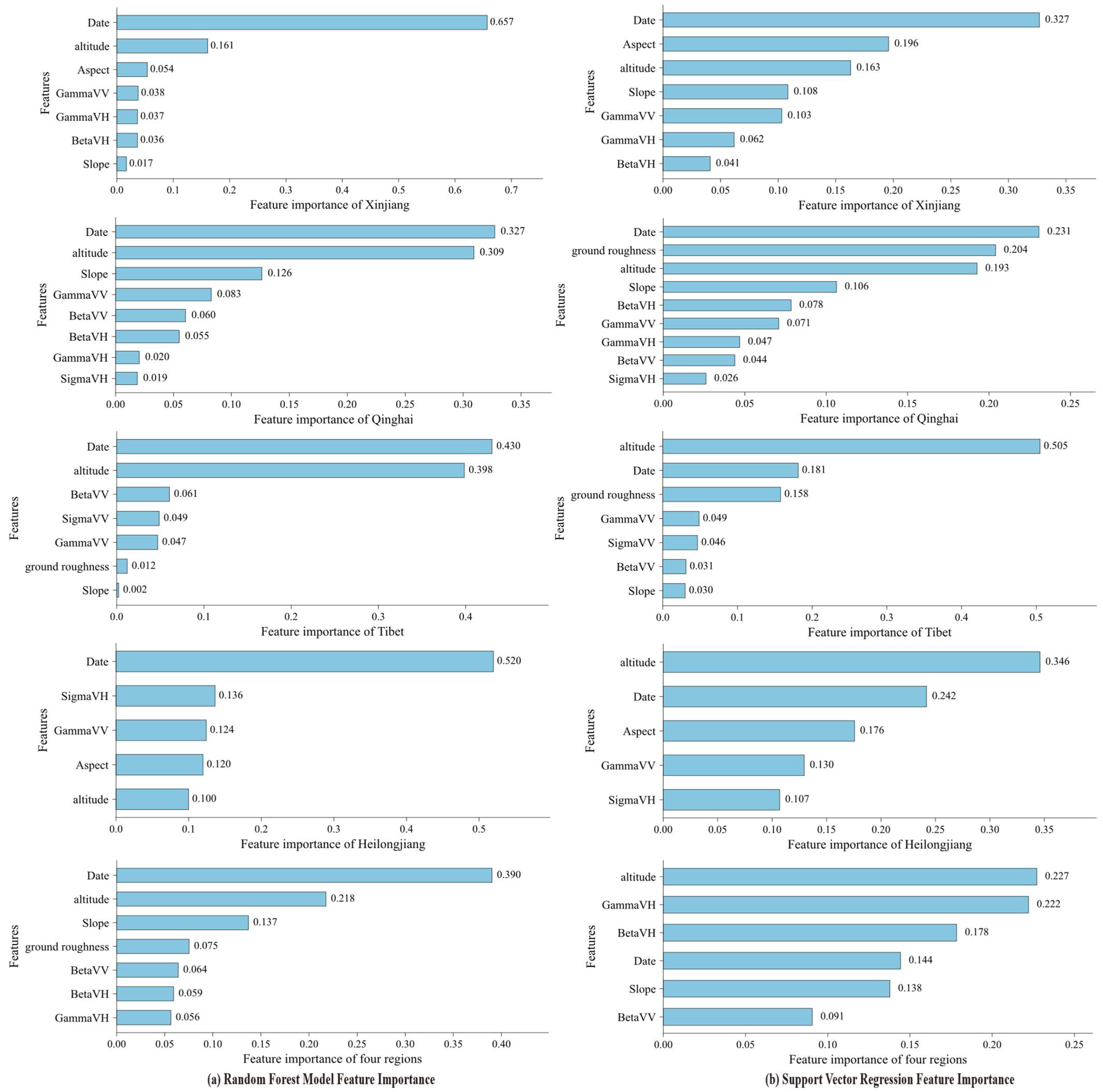
2.2.2. Selection of Optimal Feature Parameters

In model training with feature parameters, increasing feature quantity does not guarantee improved accuracy. With limited sample sizes, feature redundancy may introduce low-correlation variables that degrade model performance [48]. Proper parameter selection enables the model to better capture intrinsic data patterns, simplifies model architecture, enhances predictive capability, and improves computational efficiency.

This study implemented the Simulated Annealing (SA) algorithm for snow depth-sensitive parameter selection. SA is a heuristic optimization algorithm based on the Monte Carlo approach, with the core idea of avoiding being trapped in local optima [49]. The feature parameters consist of radar characteristics and geographic parameters, including ${\mathsf{\sigma }}_{\mathrm{VV}}$, ${\mathsf{\sigma }}_{\mathrm{VH}}$, ${\mathsf{\gamma }}_{\mathrm{VV}}$, ${\mathsf{\gamma }}_{\mathrm{VH}}$, ${\mathsf{\beta }}_{\mathrm{VV}}$, ${\mathsf{\beta }}_{\mathrm{VH}}$, ${\mathsf{\sigma }}_{\mathrm{VH}}/{\mathsf{\sigma }}_{\mathrm{VV}}$, elevation, surface roughness, slope, aspect, and date. The SA algorithm was applied to identify optimal parameter combinations for each of the four study regions and their aggregate.

The algorithm’s probabilistic acceptance criterion facilitates broad solution space exploration while preventing premature convergence to suboptimal solutions. This characteristic explains why certain region-specific selections may include seemingly less relevant features—a manifestation of the algorithm’s global optimization strategy. The complete feature selection outcomes are presented in

Table 2. Optimal feature selection results for each region.

Area	Radar Feature Parameters	Spatiotemporal Geographical Parameters
Xinjiang	${\mathsf{\beta }}_{\mathrm{VH}}$, ${\mathsf{\gamma }}_{\mathrm{VH}}$, ${\mathsf{\gamma }}_{\mathrm{VV}}$	altitude, slope, aspect, date
Qinghai	${\mathsf{\sigma }}_{\mathrm{VH}}$, ${\mathsf{\beta }}_{\mathrm{VH}}$, ${\mathsf{\gamma }}_{\mathrm{VH}}$, ${\mathsf{\beta }}_{\mathrm{VV}}$, ${\mathsf{\gamma }}_{\mathrm{VV}}$, ${\mathsf{\sigma }}_{\mathrm{VH}}/{\mathsf{\sigma }}_{\mathrm{VV}}$	altitude, slope, date
Tibet	${\mathsf{\sigma }}_{\mathrm{VV}}$, ${\mathsf{\beta }}_{\mathrm{VV}}$, ${\mathsf{\gamma }}_{\mathrm{VV}}$	altitude, ground roughness, slope, date
Heilongjiang	${\mathsf{\sigma }}_{\mathrm{VH}}$, ${\mathsf{\gamma }}_{\mathrm{VV}}$	altitude, aspect, date
Four regions	${\mathsf{\beta }}_{\mathrm{VH}}$, ${\mathsf{\gamma }}_{\mathrm{VH}}$, ${\mathsf{\beta }}_{\mathrm{VV}}$	altitude, slope, date

.

The study regions exhibit distinct topographic influences on snow distribution patterns: the Xinjiang region, with its rugged terrain and extensive mountains, shows pronounced topographic control over snow distribution, particularly in relation to slope aspect. Its radar features lack σ parameters, while geographic features include time, elevation, slope, and aspect. In the high-elevation, elevation-driven climate of Qinghai, radar features omit ${\sigma }_{\mathrm{VV}}$ and geographic variables include time, elevation, and slope. Tibet, with complex terrain and high altitudes, is strongly affected by aspect and surface roughness; its radar features exclude VH polarization and ${\sigma }_{\mathrm{VH}}/{\sigma }_{\mathrm{VV}}$, and geographic inputs are time, elevation, slope, and surface roughness. In the comparatively flat Heilongjiang region, aspect significantly affects solar radiation; radar variables are limited to ${\gamma }_{\mathrm{VV}}$ and ${\sigma }_{\mathrm{VH}}$, with geographic features of time, elevation, and aspect. Across all regions, σ-based radar parameters are absent, whereas elevation and slope consistently contribute to snow depth modeling, making time, elevation, and slope universal geographic features. Notably, ${\gamma }_{\mathrm{VV}}$ is present in all four regions, and both time and elevation are common to every study region.

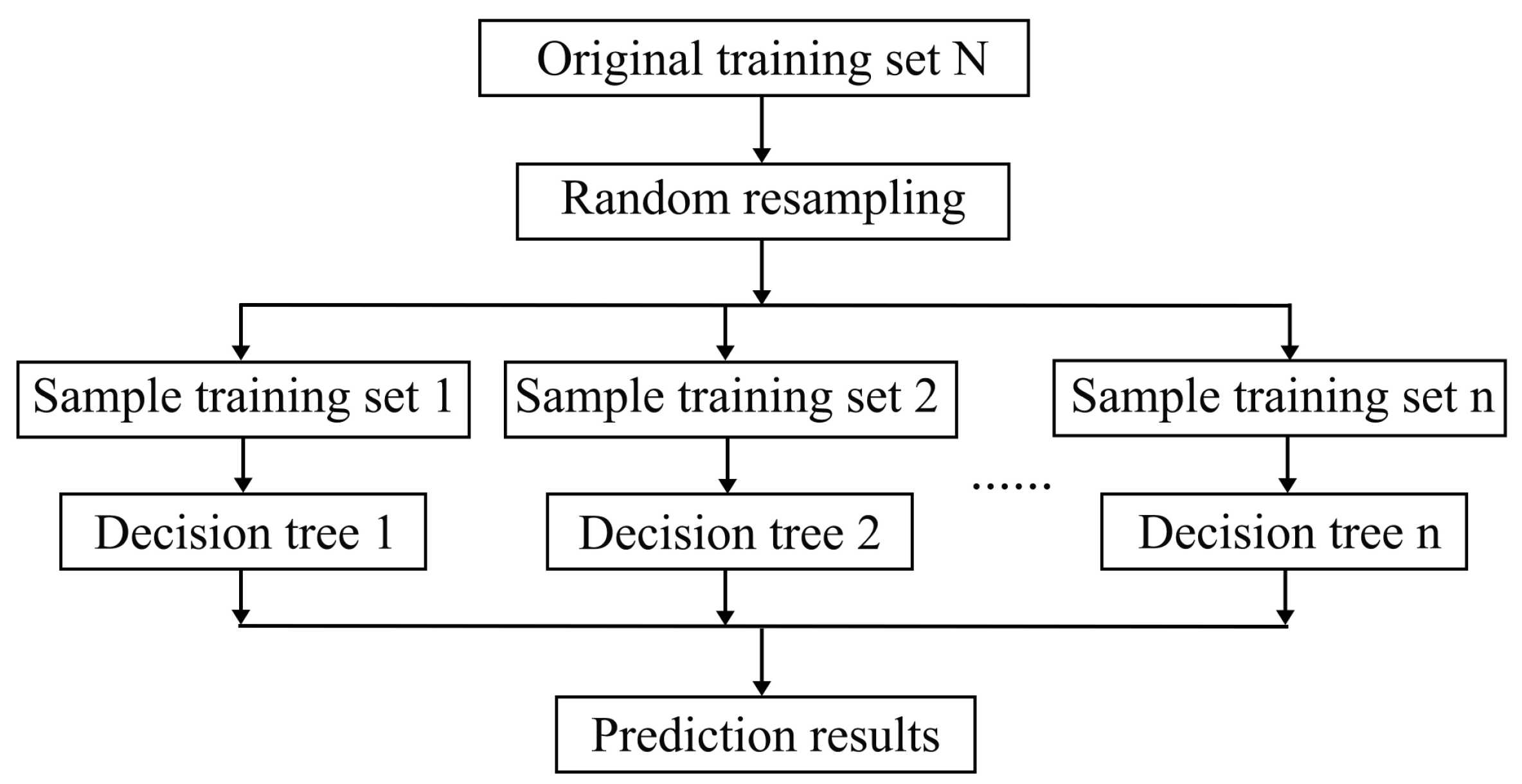
2.2.3. Random Forest Model

The random forest (RF) algorithm is an ensemble learning method based on Bagging, employing decision trees as its fundamental units for machine learning. This approach enhances prediction accuracy and model stability by aggregating predictions from multiple decision trees. The fundamental principle involves improving model performance through collective decision-making from an ensemble of trees. Each decision tree is trained on randomly sampled data subsets and randomly selected feature subsets. During prediction, the outputs of all decision trees are aggregated to produce the final prediction. The advantages of random forest include effectively reducing the risk of overfitting, improving overall prediction accuracy, and efficiently handling large-scale datasets. Given these advantages, we selected the random forest algorithm for snow depth inversion in this study with the complete workflow illustrated in Figure 2.

This study employed the RF algorithm through Python 3.12’s scikit-learn library to conduct snow depth inversion across four distinct regions and their combined dataset, encompassing various snow depth conditions. During model construction, the dataset underwent careful partitioning to maintain independence between training and testing sets while preventing data leakage. We implemented random sampling to avoid over-fitting to specific temporal periods or geographic stations, dividing the data into a 9:1 ratio where 90% serves for model training and the remaining 10% for accuracy evaluation. Parameter configuration followed Breiman’s recommendations [50], with max_features set to the square root of the total feature count to improve model randomness and stability. The max_depth parameter remained unconstrained to enable adaptive tree growth, while n_estimators underwent optimization via brute-force search across a range of 10–500 with 5-unit increments. This comprehensive parameter tuning process identified region-specific optimal configurations for different snow depth conditions, ultimately enhancing the model’s generalization capability.

2.2.4. Support Vector Regression Model

Support Vector Machine (SVM), a supervised learning method based on statistical learning theory, has demonstrated broad applicability in regression analysis [51]. This study implements a support vector regression (SVR) model for the snow depth inversion. Its core mechanism employs kernel functions to nonlinearly transform input features into a high-dimensional space, where linear regression is applied to identify the optimal hyperplane, thereby effectively addressing nonlinear problems. The model minimizes structural risk between predicted and actual values, achieving an optimal balance between global error control and model complexity.

We implemented the SVR algorithm using the scikit-learn library in Python. Prior to model training, all input features were standardized using the StandardScaler method to account for SVR’s sensitivity to feature scales. To further improve model performance, grid search with cross-validation (GridSearchCV) was employed to systematically tune the key hyperparameters of the SVR model. These hyperparameters included the regularization parameter C (which controls model complexity and overfitting risk), the kernel parameter gamma (which regulates the nonlinear mapping strength in the high-dimensional feature space), and the insensitive loss coefficient epsilon (which defines the tolerance margin for prediction errors). By constructing a hyperparameter search grid and performing K-fold cross-validation, the model was able to automatically select the optimal parameter combination, effectively balancing fitting capability and generalization performance.

2.2.5. Accuracy Validation

Three key metrics were employed to evaluate model performance: the coefficient of determination (R²), root mean square error (RMSE), and mean absolute error (MAE). R² quantifies the proportion of variance in the dependent variable that is predictable from the independent variables, with values ranging from 0 to 1, where higher values indicate superior explanatory power. Both RMSE and MAE measure prediction error magnitudes, with RMSE providing a root-mean-square measure of deviation that gives greater weight to large errors, while MAE calculates the mean absolute difference between predicted and observed values. For both error metrics, smaller values correspond to better model fit, with RMSE being particularly sensitive to outliers due to its squared term and MAE offering more robust interpretation as it represents the average absolute prediction error. The formula for calculating R² is as follows:

$$R^2=1-{\displaystyle \frac{{SS}_{res}}{{SS}_{tot}}}$$

(5)

where ${SS}_{res}$ represents the Sum of Squares Residuals, and ${SS}_{tot}$ represents the Total Sum of Squares. The calculation formulas for RMSE and MAE are as follows:

$$RMSE=\sqrt{{\displaystyle \frac{\sum _{i=1}^n{(y_i-{\widehat{y}}_i)}^2}{n}}}$$

(6)

$$MAE={\displaystyle \frac{\sum _{i=1}^n\left|y_i-{\widehat{y}}_i\right|}{n}}$$

(7)

where $y_i$ represents the actual observed values, ${\widehat{y}}_i$ represents the model-predicted values, and $n$ represents the sample size.

3. Results

This study evaluated the relative contributions of various factors in snow depth inversion by conducting feature importance analyses for both the RF and SVR models, as illustrated in Figure 3. For the RF model, feature importance was determined based on the MSE reduction attributed to each feature at decision nodes throughout the ensemble, quantifying their average contribution to enhancing predictive performance. Since SVR models lack intrinsic feature importance metrics, we employed the Permutation Importance method, which assesses feature significance by systematically randomizing individual feature values and measuring the resultant performance degradation. All importance values were normalized to sum to unity, facilitating standardized comparisons across features and between modeling approaches.

The comparative performance of these machine learning models is visualized in Figure 4 through scatter plots of predicted versus measured snow depth values. The RF model demonstrates robust predictive capability, with most data points closely aligned along the 1:1 reference line, indicating strong agreement between model estimates and ground observations. While the SVR model shows particularly accurate performance in the Qinghai region, it exhibits a consistent tendency toward slight underestimation in other study areas, suggesting potential limitations in its generalizability across diverse geographic conditions. This regional variability in model performance underscores the importance of considering spatial heterogeneity when developing snow depth inversion algorithms.

This study further validated the temporal fitting capability and stability of the machine learning models by analyzing time series of measured snow depth, existing snow depth products, and inversion results from both the RF and SVR models. Figure 5 and Figure 6 present the daily average snow depth estimates across two complete snow seasons in representative snow-covered regions, demonstrating each method’s dynamic response characteristics throughout the observation period. These temporal profiles enable direct visual comparison of methodological performance during various snow accumulation and ablation phases, revealing how each approach captures the evolution of snow depth over time. The RF model consistently tracks measured snow depth variations with high fidelity, while the SVR model shows greater temporal variability in its estimation accuracy, particularly during rapid snowmelt transitions. This temporal analysis provides critical insights into model behavior under different snowpack conditions and highlights the importance of temporal stability in snow depth inversion algorithms.

4. Discussion

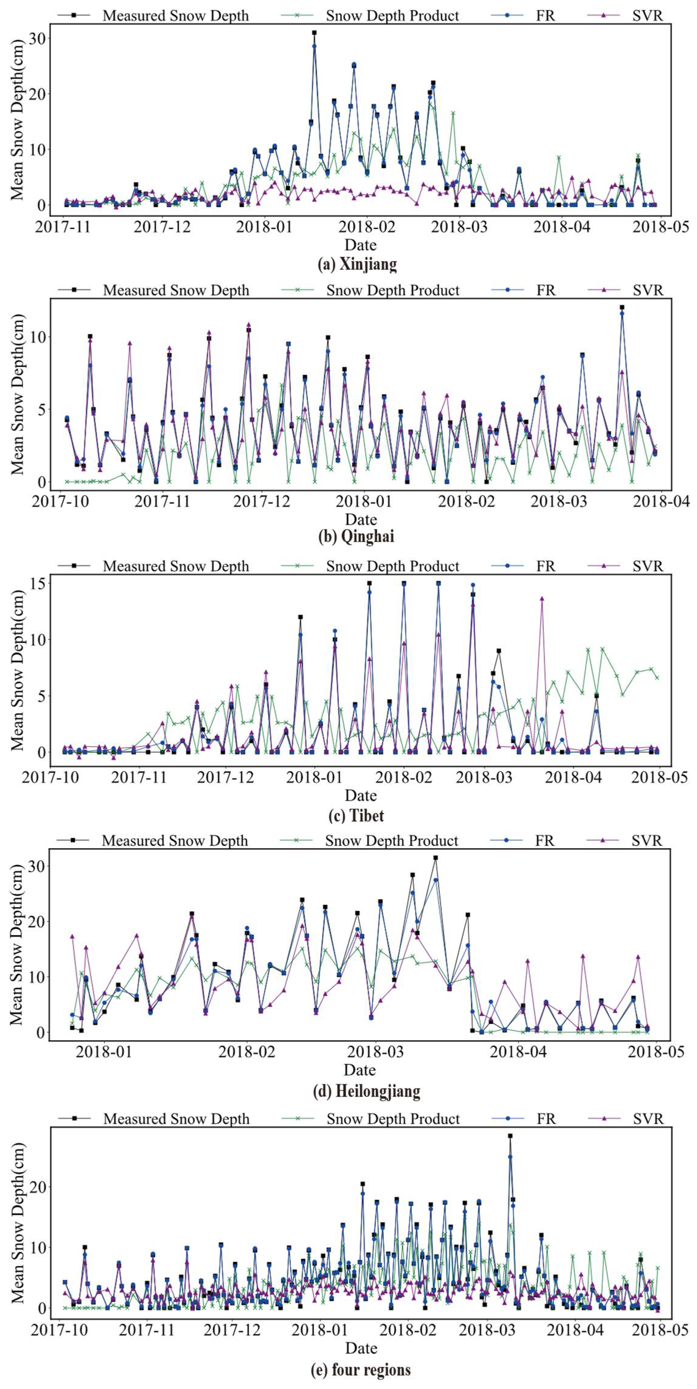
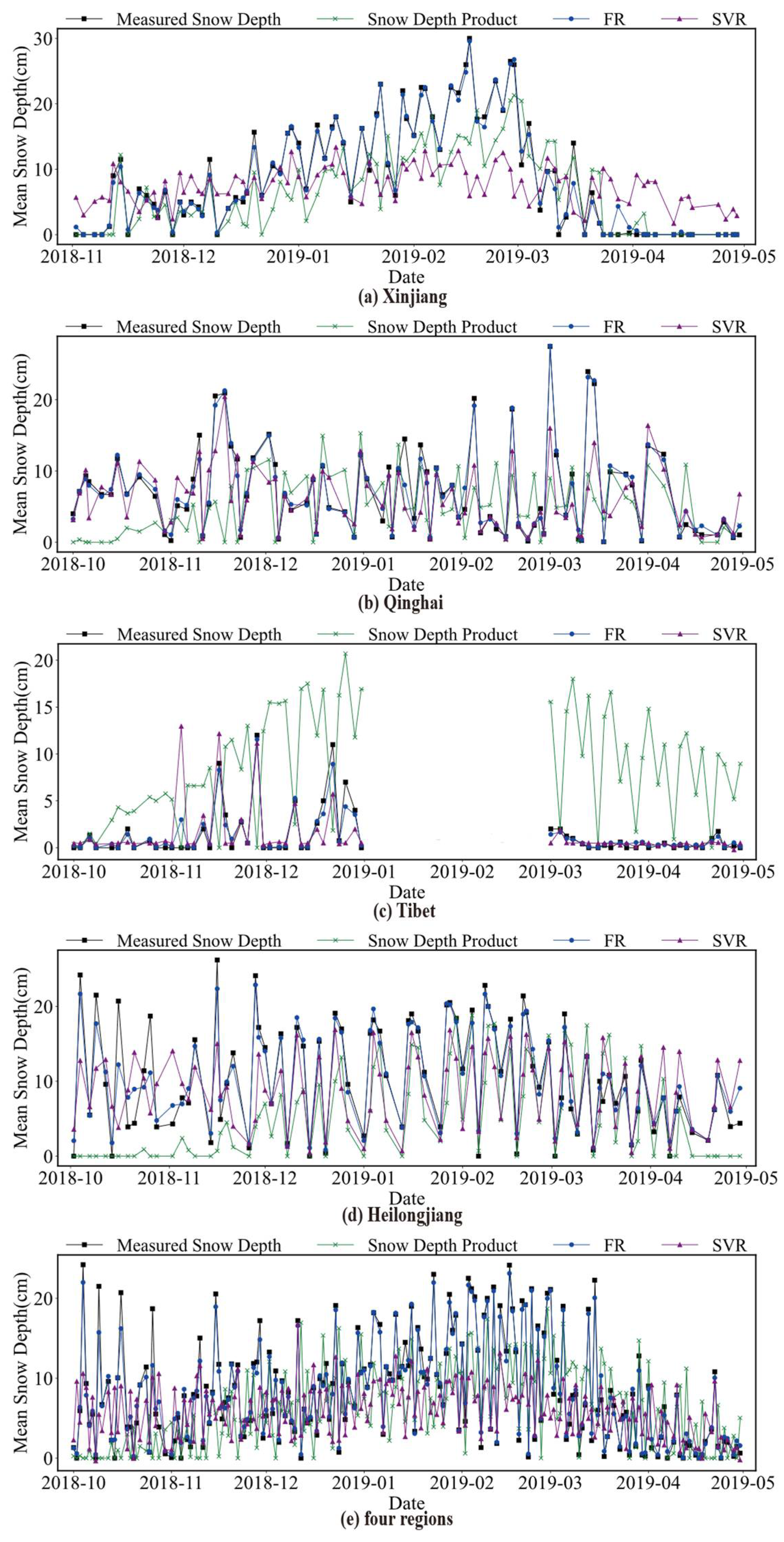
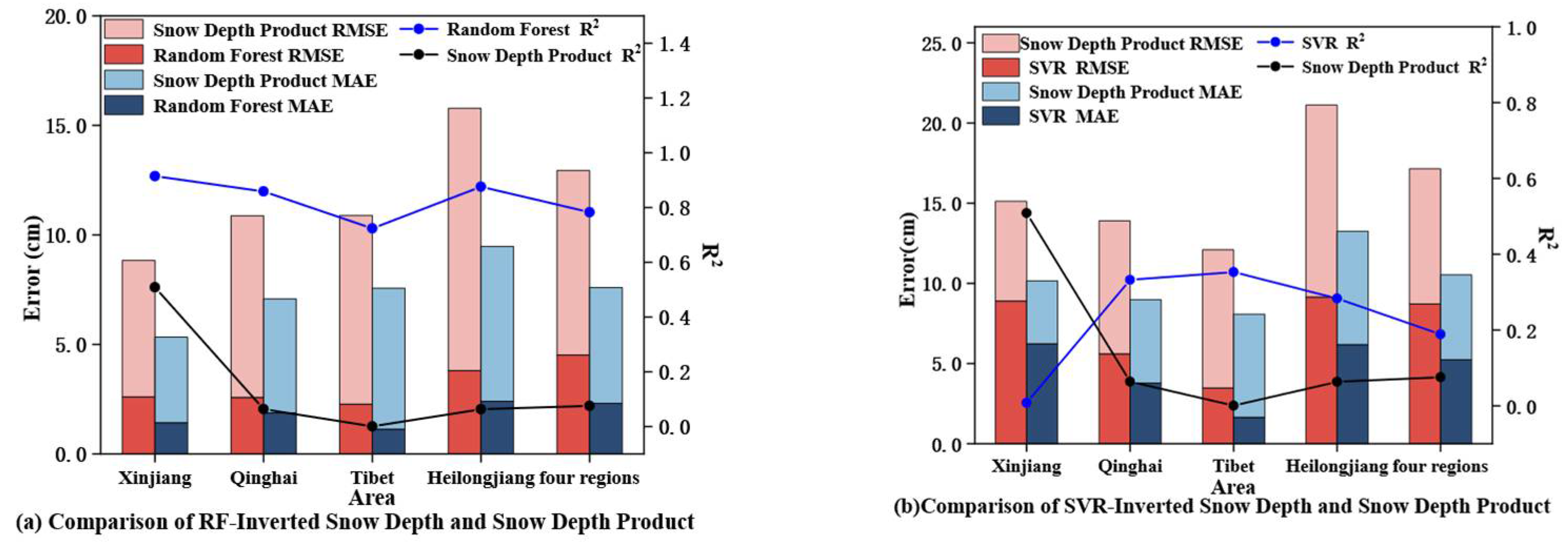
4.1. Comparison of Model Inversion Results with Snow Depth Product Results

This study employs the RF and SVR models for snow depth inversion and comprehensively evaluates their performance against the China Snow Depth Long Time Series Dataset during 2017–2019. Through quantitative assessment using three key metrics—R², RMSE, and MAE—we systematically compare model performance across different geographical regions.

The RF model demonstrates superior accuracy across all study areas, consistently outperforming the benchmark snow depth product. As illustrated in Figure 7, the RF model achieves R² values exceeding 0.7 in all regions, with particularly outstanding performance in Xinjiang (R² = 0.91, RMSE = 2.62 cm, MAE = 1.42 cm). While Tibet shows relatively lower accuracy (R² = 0.72, RMSE = 2.27 cm, MAE = 1.13 cm), it still significantly surpasses the reference product. Qinghai (R² = 0.86) and Heilongjiang (R² = 0.88) exhibit strong performance, with the combined regional analysis yielding an overall R² of 0.78 (RMSE = 4.51 cm, MAE = 2.31 cm). Notably, the reference product displays systematic underestimation in most regions, except Xinjiang.

In contrast, the SVR model shows limited predictive capability and regional consistency. While achieving modest improvements over the reference product in Qinghai (R² = 0.33) and Tibet (R² = 0.35), its performance proves inadequate in Xinjiang (R² = 0.01) and Heilongjiang (R² = 0.28). The model’s elevated error metrics (RMSE up to 9.14 cm in Heilongjiang) and poor overall accuracy (combined R² = 0.19) reveal fundamental limitations in its applicability for snow depth inversion. These results suggest that while the SVR approach can capture certain terrain-specific patterns, its general utility for regional-scale snow depth estimation remains constrained compared to the robust performance of the RF methodology.

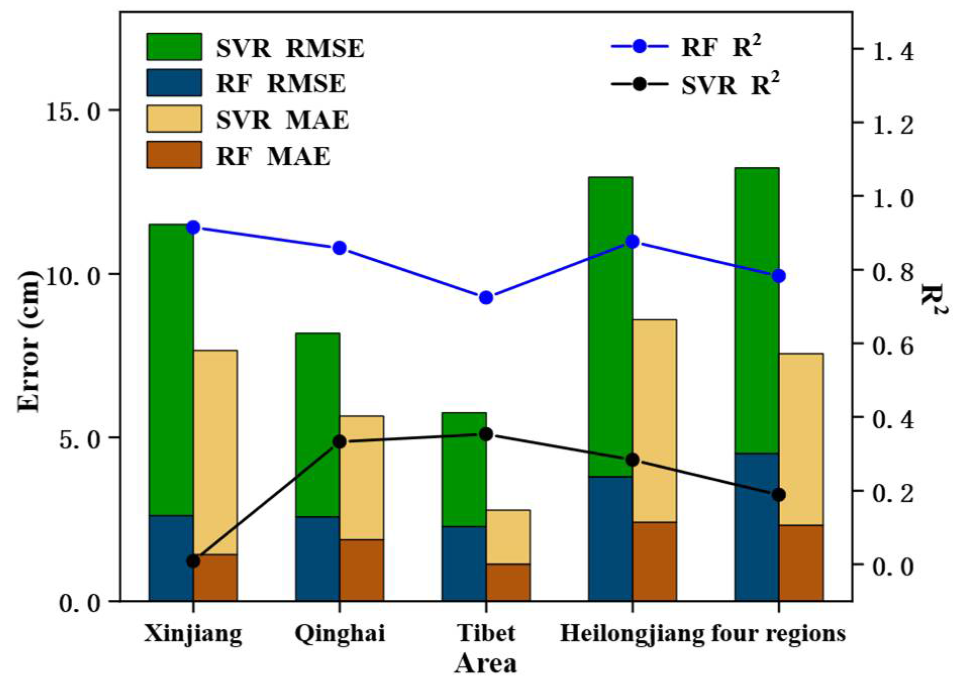
4.2. Comparison of Model Inversion Results

Figure 8 demonstrates the consistent superiority of the RF model over SVR across all evaluated regions, exhibiting enhanced fitting accuracy, reduced error metrics, and superior generalization capacity. The RF model achieves exceptional performance in Xinjiang with an R² of 0.92, dramatically outperforming SVR’s negligible explanatory power (R² = 0.01). This regional dominance is further evidenced by substantially lower error metrics (RF: RMSE = 2.61 cm, MAE = 1.42 cm versus SVR: RMSE = 8.9 cm, MAE = 6.24 cm), revealing fundamental limitations in SVR’s predictive capability for this environment.

While SVR shows modest improvements over conventional snow depth products in Qinghai (R² = 0.33, RMSE = 5.60 cm) and Tibet (R² = 0.35, RMSE = 3.48 cm), its performance remains markedly inferior to the RF model’s robust accuracy (Qinghai: R² = 0.86, RMSE = 2.58 cm; Tibet: R² = 0.72, RMSE = 2.27 cm). The northeast region highlights SVR’s particular challenges in handling variable snow conditions, where its R² of 0.28 and RMSE of 9.14 cm compare unfavorably with RF’s 0.88 R² and 3.81 cm RMSE.

Aggregate analysis across all regions confirms RF’s comprehensive advantages, achieving an overall R² of 0.78 (versus SVR’s 0.19) with substantially lower error magnitudes (RF: RMSE = 4.51 cm, MAE = 2.31 cm; SVR: RMSE = 8.72 cm, MAE = 5.25 cm). These results collectively establish RF as a more reliable and stable methodology for multi-regional snow depth inversion, capable of maintaining consistent accuracy across diverse geographical and snowpack conditions where SVR demonstrates significant performance variability.

In summary, the RF model demonstrates comprehensive superiority over SVR in this snow depth inversion study, exhibiting enhanced feature representation and superior nonlinear modeling capabilities. This advantage proves particularly significant in regions characterized by complex snow distribution patterns or pronounced topographic variations. Conversely, the SVR model shows notable limitations due to its sensitivity to parameter selection and tendency toward over-fitting when processing high-dimensional feature spaces and large sample sizes. These inherent constraints manifest as inconsistent performance across most study regions and ultimately restrict the model’s practical utility for large-scale snow depth inversion applications. The comparative analysis clearly establishes RF as the more robust and reliable approach for regional snow depth estimation tasks.

5. Conclusions

This study utilized Sentinel-1 radar feature data combined with geographic parameters to develop an advanced snow depth inversion approach. The methodology involved three key phases: first, optimal feature selection was performed using a simulated annealing algorithm; second, machine learning techniques, including RF and SVR, were implemented for snow depth estimation at representative Chinese snow monitoring stations; and third, comprehensive validation was conducted by comparing the algorithm outputs with existing snow depth products. Through this rigorous analytical process, we have drawn the following principal conclusions:

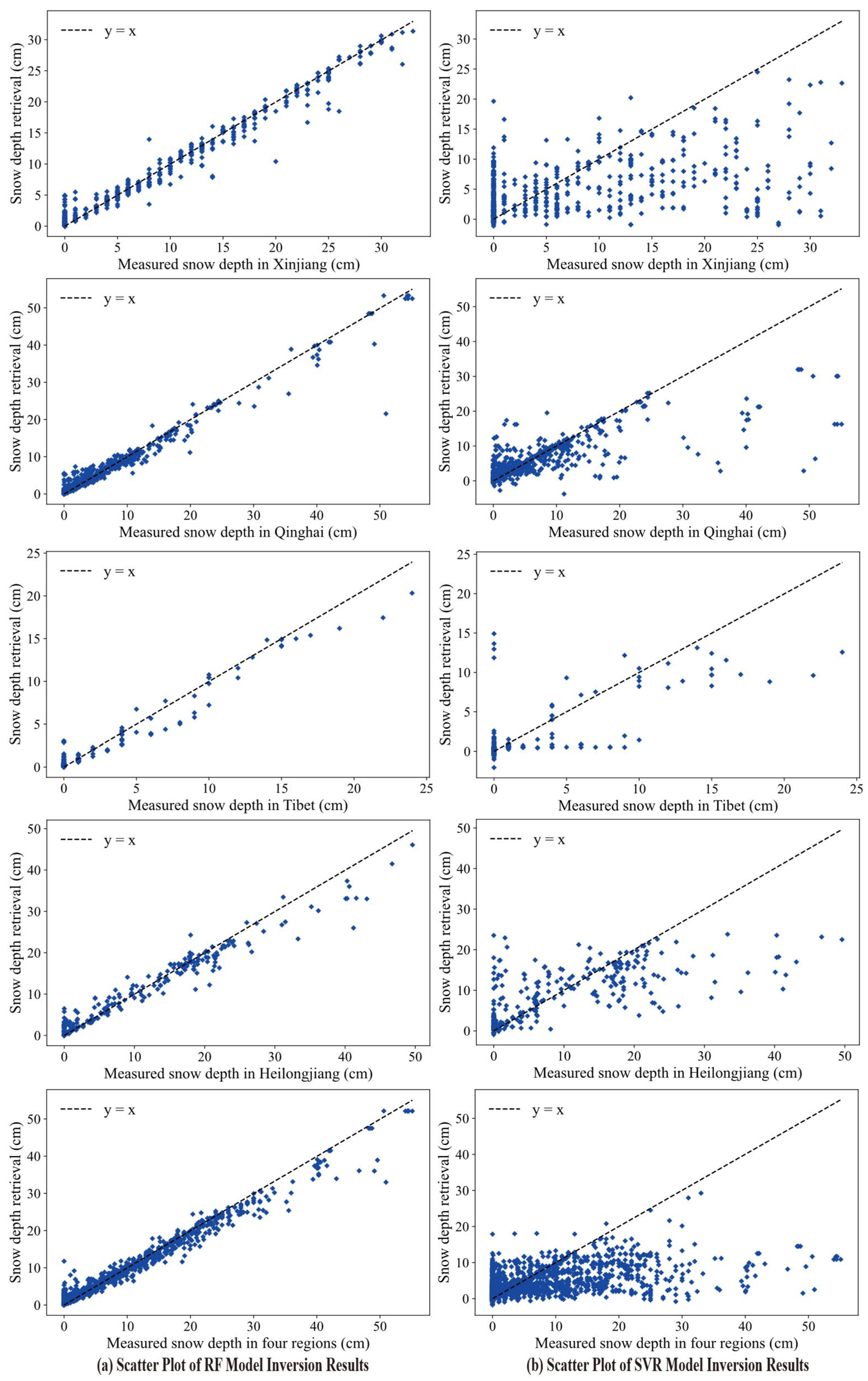
• The RF model demonstrates superior inversion accuracy and regional adaptability, achieving consistently high goodness-of-fit values (R²) across all study areas, most notably in Xinjiang (R² = 0.915) while maintaining strong overall performance (R² = 0.78) across all four regions. This represents a significant improvement over both SVR and conventional snow depth products, as evidenced by substantially lower RMSE and MAE values that confirm the RF model’s enhanced generalization capability under diverse terrain and snow conditions;
• While the SVR model shows marginal improvements over snow depth products in certain regions (Qinghai, Tibet, and Heilongjiang), its overall performance proves inconsistent, particularly in Xinjiang, where it underperforms even the baseline products. The model’s generally elevated error metrics (RMSE and MAE) across all regions highlight fundamental limitations in prediction accuracy and stability compared to the RF approach;
• Comparative analysis reveals the RF model’s distinct advantages over existing snow depth products, which exhibit systematic underestimation/overestimation issues evidenced by negative R² values in some regions. The RF methodology’s superior accuracy and reliability establish it as a valuable reference for high-precision snow depth inversion applications;
• Notably, region-specific modeling demonstrates clear advantages over unified approaches, with the RF model’s aggregate regional performance (R² = 0.78) falling below the average accuracy of individual regional models. This performance gap becomes even more pronounced for SVR (overall R² = 0.09), emphasizing the importance of accounting for regional variations in terrain, climate, and vegetation characteristics through localized factor selection and modeling strategies.

In conclusion, the RF model emerges as the superior solution for snow depth inversion, combining robust accuracy with exceptional adaptability across complex terrains and multi-regional scales. While current results demonstrate significant progress, challenges remain regarding snow layer structure effects on radar signals and the optimal integration of auxiliary parameters. Future research directions should explore multi-source remote sensing data fusion and advanced deep learning architectures to further enhance model precision and interpretability, ultimately strengthening support for snowpack monitoring and related hydrological and climate studies.

References

1. Grippa, M.; Mognard, N.; Le Toan, T.; Josberger, E.G. Siberia Snow Depth Climatology Derived from SSM/I Data Using a Combined Dynamic and Static Algorithm. Remote Sens. Environ. 2004, 93, 30–41. [Google Scholar] [CrossRef]
2. Che, T.; Li, X.; Gao, F. Estimation of Snow Water Equivalent in the Tibetan Plateau Using Passive Microwave Remote Sensing Data (SSM/I). J. Glaciol. Geocryol. 2004, 26, 363–368. [Google Scholar] [CrossRef]
3. Chen, X.; Li, X.; Wang, G.; Zhao, K.; Zheng, X.; Jiang, T. Based on Snow Cover Survey Data of Accuracy Verification and Analysis of Passive Microwave Snow Cover Remote Sensing Products in Northeast China. Remote Sens. Technol. Appl. 2019, 34, 1181–1189. [Google Scholar]
4. Chen, F.; Chang, L.; Feng, G. Inversion of Snow Depth in Alaska Based on GNSS-R Technology and Its Application. Chin. J. Polar Res. 2023, 35, 197–211. [Google Scholar] [CrossRef]
5. Che, T.; Li, X.; Jin, R.; Huang, C. Assimilating Passive Microwave Remote Sensing Data into a Land Surface Model to Improve the Estimation of Snow Depth. Remote Sens. Environ. 2014, 143, 54–63. [Google Scholar] [CrossRef]
6. Lu, X.; Wang, X.; Cui, C.; Xie, G. Snow Depth Retrieval Based on AMSR-E Data in Northern Xinjiang Region, China. J. Glaciol. Geocryol. 2013, 35, 40–47. [Google Scholar]
7. Deng, G.; Tang, Z.; Dong, C.; Shao, D.; Wang, X. Development and Evaluation of a Cloud-Gap-Filled MODIS Normalized Difference Snow Index Product over High Mountain Asia. Remote Sens. 2024, 16, 192. [Google Scholar] [CrossRef]
8. Wang, J.; Tang, Z.; Deng, G.; Hu, G.; You, Y.; Zhao, Y. Landsat Satellites Observed Dynamics of Snowline Altitude at the End of the Melting Season, Himalayas, 1991–2022. Remote Sens. 2023, 15, 2534. [Google Scholar] [CrossRef]
9. Min, W.; Pen, J.; Li, S. The Evaluation of FY-3C Snow Products in the Tibetan Plateau. Remote Sens. Nat. Resour. 2021, 33, 145–151. [Google Scholar] [CrossRef]
10. Liang, Z.; Yu, Z.; Hong, Y.; Yamin, H.; Ming, X.; Jian, G. A dynamic approach to retrieving snow depth based on the technology of integrating satellite remote sensing and in situ data. Acta Meteorol. Sin. 2013, 71, 769–782. [Google Scholar] [CrossRef]
11. Tanis, C.M.; Lindgren, E.; Frey, A.; Latva, L.; Arslan, A.N.; Luojus, K. Use of Webcams in Support of Operational Snow Monitoring. Geosciences 2023, 13, 92. [Google Scholar] [CrossRef]
12. Jenssen, R.; Eckerstorfer, M.; Jacobsen, S. Drone-Mounted Ultrawideband Radar for Retrieval of Snowpack Properties. IEEE Trans. Instrum. Meas. 2020, 69, 221–230. [Google Scholar] [CrossRef]
13. Gao, F.; Li, X.; Armstrong, R.; Wang, J.; Che, T.; Xu, W. Operational Snow Monitoring on the Tibetan Plateau by Using SSM/I Data and Algorithm Validation. In Proceedings of the Third International Asia-Pacific Environmental Remote Sensing Remote Sensing of the Atmosphere, Ocean, Environment, and Space, Hangzhou, China, 30 April 2003; Volume 4894, pp. 456–463. [Google Scholar]
14. Jiang, L.; Wang, P.; Zhang, L.; Yang, H.; Yang, J. Improvement of Snow Depth Retrieval for FY3B-MWRI in China. Sci. China Earth Sci. 2014, 57, 1278–1292. [Google Scholar] [CrossRef]
15. Gao, S.; Wu, Y.; Qian, B. Retrieval of Snow Depth from FY-3B/MWRI Data over the Qinghai-Tibetan Plateau. Prog. Geophys. 2020, 35, 399–405. [Google Scholar] [CrossRef]
16. Josberger, E.; Mognard, N. Passive Microwave Snow Depth Algorithm with a Proxy for Snow Metamorphism. Hydrol. Process. 2002, 16, 1557–1568. [Google Scholar] [CrossRef]
17. Wu, J.; Yao, T.; Dai, Y.; Chen, W. Evaluation of Passive Microwave Snow-Depth Retrieval Algorithm in Selin Co and Nam Co. Remote Sens. Technol. Appl. 2022, 37, 1339–1349. [Google Scholar]
18. Xiao, X.; Zhang, T. Passive Microwave Remote Sensing of Snow Depth and Snow Water Equivalent: Overview. Adv. Earth Sci. 2018, 33, 590. [Google Scholar] [CrossRef]
19. Wen, J.; Dai, M.; Jean, P. Extent and Depth of Snow Cover over the Nyainqêntanghla Range Derived from ASAR and MODIS Data. J. Glaciol. Geocryol. 2006, 28, 54–61. [Google Scholar]
20. Pulliainen, J.; Grandell, J.; Hallikainen, M. HUT Snow Emission Model and Its Applicability to Snow Water Equivalent Retrieval. IEEE Trans. Geosci. Remote Sens. 1999, 37, 1378–1390. [Google Scholar] [CrossRef]
21. Tsang, L.; Chen, C.; Chang, A.T.C.; Guo, J.; Ding, K. Dense Media Radiative Transfer Theory Based on Quasicrystalline Approximation with Applications to Passive Microwave Remote Sensing of Snow. Radio Sci. 2000, 35, 731–749. [Google Scholar] [CrossRef]
22. Che, T.; Dai, L.; Zheng, X.; Li, X.; Zhao, K. Estimation of snow depth from passive microwave brightness temperature data in forest regions of northeast China. Remote Sens. Environ. 2016, 183, 334–349. [Google Scholar] [CrossRef]
23. Deng, G.; Liu, X.; Shen, Q.; Zhang, T.; Chen, Q.; Tang, Z. Remote Sensing Data Assimilation to Improve the Seasonal Snow Cover Simulations Over the Heihe River Basin, Northwest China. Int. J. Climatol. 2024, 44, 5621–5640. [Google Scholar] [CrossRef]
24. Bi, Y.; He, W.; Long, F.; Chen, H.; Li, C. Improvement of the Snow-Depth Retrieval Algorithm Using Passive Microwave Remote Sensing over the Arxan Region Inner Mongolia. Clim. Environ. Res. 2020, 25, 410–418. [Google Scholar] [CrossRef]
25. Yao, H.; Zhang, Y.; Jiang, L.; Ewe, H.; Ng, M. Snow Parameters Inversion from Passive Microwave Remote Sensing Measurements by Deep Convolutional Neural Networks. Sensors 2022, 22, 4769. [Google Scholar] [CrossRef] [PubMed]
26. Wei, Y.; Li, X.; Gu, L.; Zheng, X.; Jiang, T.; Zheng, Z. A Fine-Resolution Snow Depth Retrieval Algorithm From Enhanced-Resolution Passive Microwave Brightness Temperature Using Machine Learning in Northeast China. IEEE Geosci. Remote Sens. Lett. 2022, 19, 1–5. [Google Scholar] [CrossRef]
27. Li, Q.; Yang, T.; Zhang, F.; Qi, Z.; Li, L. Snow Depth Reconstruction over Last Century: Trend and Distribution in the Tianshan Mountains, China. Glob. Planet. Change 2019, 173, 73–82. [Google Scholar] [CrossRef]
28. Xiao, X.; Zhang, T.; Zhong, X.; Shao, W.; Li, X. Support Vector Regression Snow-Depth Retrieval Algorithm Using Passive Microwave Remote Sensing Data. Remote Sens. Environ. 2018, 210, 48–64. [Google Scholar] [CrossRef]
29. Zhou, Z.; Zhu, L.; Zhang, Y.; Kan, X.; Liu, X.; Cao, H.; Wang, J. Downscaling Machine Learning Snow Depth Inversion on the Qinghai-Xizang Plateau Based on FY-3B Passive Microwave Data. J. Glaciol. Geocryol. 2024, 46, 539–554. [Google Scholar] [CrossRef]
30. Dai, L.; Che, T. Estimating snow depth or snow water equivalent from space. Sci. Cold Arid. Reg. 2022, 14, 79–90. [Google Scholar]
31. Yu, X.; Hu, X.; Wang, G.; Wang, K.; Chen, X. Machine-Learning Estimation of Snow Depth in 2021 Texas Statewide Winter Storm Using SAR Imagery. Geophys. Res. Lett. 2022, 49, e99119. [Google Scholar] [CrossRef]
32. Yang, Y.; Fang, S.; Wu, H.; Du, J.; Wang, X.; Chen, R.; Liu, Y.; Wang, H. High-Resolution Inversion Method for the Snow Water Equivalent Based on the GF-3 Satellite and Optimized EQeau Model. Remote Sens. 2022, 14, 4931. [Google Scholar] [CrossRef]
33. Dozier, J.; Shi, J. Estimation of Snow Water Equivalence Using SIR-C/X-SAR. I. Inferring Snow Density and Subsurface Properties. IEEE Trans. Geosci. Remote Sens. 2000, 38, 2465–2474. [Google Scholar] [CrossRef]
34. Dozier, J.; Shi, J. Estimation of Snow Water Equivalence Using SIR-C/X-SAR. II. Inferring Snow Depth and Particle Size. IEEE Trans. Geosci. Remote Sens. 2000, 38, 2475–2488. [Google Scholar] [CrossRef]
35. Gorelick, N.; Hancher, M.; Dixon, M.; Ilyushchenko, S.; Thau, D.; Moore, R. Google Earth Engine: Planetary-Scale Geospatial Analysis for Everyone. Remote Sens. Environ. 2017, 202, 18–27. [Google Scholar] [CrossRef]
36. European Space Agency (ESA). Sentinel-1 SAR GRD: C-Band Synthetic Aperture Radar Ground Range Detected. Google Earth Engine Dataset. 2023. Available online: https://developers.google.com/earth-engine/datasets/catalog/COPERNICUS_S1_GRD (accessed on 6 July 2025).
37. Farr, T.; Rosen, P.; Caro, E.; Crippen, R.; Duren, R.; Hensley, S.; Kobrick, M.; Paller, M.; Rodriguez, E.; Roth, L.; et al. The Shuttle Radar Topography Mission. Rev. Geophys. 2007, 45, RG2004. [Google Scholar] [CrossRef]
38. Li, L.; Che, T.; Liu, Y.; Li, X. Snow Depth Dataset from Common Station in the Typical Regions of China during 2017–2019. 2021. [Google Scholar] [CrossRef]
39. Che, T.; Dai, L.; Li, X. Long-Term Series of Daily Snow Depth Dataset in China (1979–2024). Natl. Tibet. Plateau Data Cent. 2015. [Google Scholar] [CrossRef]
40. King, J.; Kelly, R.; Kasurak, A.; Duguay, C.; Gunn, G.; Rutter, N.; Watts, T.; Derksen, C. Spatio-Temporal Influence of Tundra Snow Properties on Ku-Band (17.2 GHz) Backscatter. J. Glaciol. 2015, 61, 267–279. [Google Scholar] [CrossRef]
41. Lemmetyinen, J.; Derksen, C.; Toose, P.; Proksch, M.; Pulliainen, J.; Kontu, A.; Rautiainen, K.; Seppänen, J.; Hallikainen, M. Simulating Seasonally and Spatially Varying Snow Cover Brightness Temperature Using HUT Snow Emission Model and Retrieval of a Microwave Effective Grain Size. Remote Sens. Environ. 2015, 156, 71–95. [Google Scholar] [CrossRef]
42. Loew, A.; Mauser, W. Generation of Geometrically and Radiometrically Terrain Corrected SAR Image Products. Remote Sens. Environ. 2007, 106, 337–349. [Google Scholar] [CrossRef]
43. Lievens, H.; Demuzere, M.; Marshall, H.-P.; Reichle, R.H.; Brucker, L.; Brangers, I.; de Rosnay, P.; Dumont, M.; Girotto, M.; Immerzeel, W.W.; et al. Snow Depth Variability in the Northern Hemisphere Mountains Observed from Space. Nat. Commun. 2019, 10, 4629. [Google Scholar] [CrossRef] [PubMed]
44. Bo, Y.; Feng, X. The Retrieval of Snow-Depth Using SSM/I Remotely Sensed Data and Its Results Assessment in Qinghai-Xizang (Tibet) Plateau. In Proceedings of the IGARSS 2000, IEEE 2000 International Geoscience and Remote Sensing Symposium, Honolulu, HI, USA, 24–28 July 2000; Volume 2, pp. 509–511. [Google Scholar] [CrossRef]
45. Deng, G.; Tang, Z.; Hu, G.; Wang, J.; Sang, G.; Li, J. Spatiotemporal Dynamics of Snowline Altitude and Their Responses to Climate Change in the Tienshan Mountains, Central Asia, during 2001–2019. Sustainability 2021, 13, 3992. [Google Scholar] [CrossRef]
46. Tang, Z.; Wang, X.; Deng, G.; Wang, X.; Jiang, Z.; Sang, G. Spatiotemporal Variation of Snowline Altitude at the End of Melting Season across High Mountain Asia, Using MODIS Snow Cover Product. Adv. Space Res. 2020, 66, 2629–2645. [Google Scholar] [CrossRef]
47. Wang, J.; Wang, Y.; Zhou, M.; Liu, C.; Huang, X. Retrieved Snow Depth over the Tibetan Plateau Using Random Forest Algorithm with AMSR2 Passive Microwave Data. J. Glaciol. Geocryol. 2020, 42, 1077–1086. [Google Scholar] [CrossRef]
48. Liu, G.; Jiang, X.; Tang, B. Application of Feature Optimization and Convolutional Neural Network in Crop Classification. J. Geo-Inf. Sci. 2021, 23, 1071–1081. [Google Scholar] [CrossRef]
49. Habibi, A.; Delavar, M.R.; Nazari, B.; Pirasteh, S.; Sadeghian, M.S. A Novel Approach for Flood Hazard Assessment Using Hybridized Ensemble Models and Feature Selection Algorithms. Int. J. Appl. Earth Obs. Geoinf. 2023, 122, 103443. [Google Scholar] [CrossRef]
50. Breiman, L. Random Forests. Mach. Learn. 2001, 45, 5–32. [Google Scholar] [CrossRef]
51. Tedesco, M.; Pulliainen, J.; Takala, M.; Hallikainen, M.; Pampaloni, P. Artificial Neural Network-Based Techniques for the Retrieval of SWE and Snow Depth from SSM/I Data. Remote Sens. Environ. 2004, 90, 76–85. [Google Scholar] [CrossRef]
Figure 1. Distribution of typical snow-covered area stations.
Remotesensing 17 02584 g001
Figure 2. Random forest algorithm workflow.
Remotesensing 17 02584 g002
Figure 3. Feature importance of machine learning models. (a) Feature importance of random forest models in different regions; (b) feature importance of support vector regression models in different regions.
Remotesensing 17 02584 g003
Figure 4. Scatter plot of snow depth inversion results from machine learning models. (a) Scatter plot of snow depth inversion using RF model; (b) scatter plot of snow depth inversion using SVR model.
Remotesensing 17 02584 g004
Figure 5. Daily average snow depth time series for each region during the first snow season. (a) Daily average snow depth time series for each subregion in Xinjiang during the first snow season; (b) daily average snow depth time series for each subregion in Qinghai during the first snow season; (c) daily average snow depth time series for each subregion in Tibet during the first snow season; (d) daily average snow depth time series for each subregion in Heilongjiang during the first snow season; (e) daily average snow depth time series for each region in the four areas during the first snow season.
Remotesensing 17 02584 g005
Figure 6. Daily average snow depth time series for each region during the second snow season. (a) Daily average snow depth time Series for Each Subregion in Xinjiang during the second snow season; (b) daily average snow depth time series for each subregion in Qinghai during the second snow season; (c) daily average snow depth time series for each subregion in Tibet during the second snow season; (d) daily average snow depth time series for each subregion in Heilongjiang during the second snow season; (e) daily average snow depth time series for each region in the four areas during the second snow season.
Remotesensing 17 02584 g006
Figure 7. Comparison of the retrieval results from the two models with the snow depth product results. (a) Comparison of RF-Inverted Snow Depth and snow depth product; (b) comparison of SVR-Inverted Snow Depth and snow depth product.
Remotesensing 17 02584 g007
Figure 8. Accuracy comparison of random forest and support vector regression models.
Remotesensing 17 02584 g008