Multi-Head Graph Attention Adversarial Autoencoder Network for Unsupervised Change Detection Using Heterogeneous Remote Sensing Images

Abstract

Heterogeneous remote sensing images, acquired from different sensors, exhibit significant variations in data structure, resolution, and radiometric characteristics. These inherent heterogeneities present substantial challenges for change detection, a task that involves identifying changes in a target area by analyzing multi-temporal images. To address this issue, we propose the Multi-Head Graph Attention Mechanism (MHGAN), designed to achieve accurate detection of surface changes in heterogeneous remote sensing images. The MHGAN employs a bidirectional adversarial convolutional autoencoder network to reconstruct and perform style transformation of heterogeneous images. Unlike existing unidirectional translation frameworks (e.g., CycleGAN), our approach simultaneously aligns features in both domains through multi-head graph attention and dynamic kernel width estimation, effectively reducing false changes caused by sensor heterogeneity. The network training is constrained by four loss functions: reconstruction loss, code correlation loss, graph attention loss, and adversarial loss, which together guide the alignment of heterogeneous images into a unified data domain. The code correlation loss enforces consistency in feature representations at the encoding layer, while a density-based kernel width estimation method enhances the capture of both local and global changes. The graph attention loss models the relationships between features and images, improving the representation of consistent regions across bitemporal images. Additionally, adversarial loss promotes style consistency within the shared domain. Our bidirectional adversarial convolutional autoencoder simultaneously aligns features across both domains. This bilateral structure mitigates the information loss associated with one-way mappings, enabling more accurate style transformation and reducing false change detections caused by sensor heterogeneity, which represents a key advantage over existing unidirectional methods. Compared with state-of-the-art methods for heterogeneous change detection, the MHGAN demonstrates superior performance in both qualitative and quantitative evaluations across four benchmark heterogeneous remote sensing datasets.

1. Introduction

Remote sensing image change detection focuses on analyzing dual-temporal images of the same geographic area to accurately identify and quantify changes within the observed region [1]. Traditionally, this task has relied on homogeneous images—those acquired by the same sensor [2]—and has been widely applied in fields such as remote sensing information processing [3], computer vision [4], urban development monitoring [5], deforestation assessment [6], and land cover change analysis [7,8]. However, in many practical scenarios, obtaining homogeneous imagery is challenging due to sensor limitations and varying acquisition conditions. With the rapid advancement of satellite and imaging technologies, the availability of large-scale and diverse remote sensing data has significantly increased, making heterogeneous remote sensing image change detection—utilizing images from different sensors—a timely and practical alternative [9,10]. This approach not only meets the real-world demand for rapid and effective change detection, especially in emergency disaster assessment, but also benefits from the complementarity of diverse data sources. Consequently, there is a growing need to develop fast, automated, and unsupervised heterogeneous change detection methods that can harness these diverse datasets for robust and efficient surface change monitoring.

Currently, heterogeneous change detection (CD) methods can be broadly classified into traditional methods and deep-learning-based methods. Traditional methods mainly rely on images similarity measures and classification-based approaches. Image similarity measures detect change areas by quantifying the difference or similarity between images, with typical methods including analysis based on correlation coefficients, mutual information, and other metrics. Examples include post-classification comparison [11] and multi-temporal segmentation and compound classification (MS-CC) [12]. However, these methods are often sensitive to data heterogeneity and struggle to address complex change relationships between multi-sensor or multi-modal data. Classification-based methods, on the other hand, classify the images first and then compare the classification results to detect change areas. Examples include Sorted Histogram Distance (SHD) [13] and Pixel Pair (PP) methods [14]. While these methods can effectively detect specific changes, classification errors and heterogeneity significantly impact the performance of the PCC method in practical applications. Additionally, as the complexity of data increases, these methods face challenges in terms of computational efficiency and robustness, making it difficult to meet the needs of high-resolution data. In recent years, deep learning methods, with their powerful feature extraction capabilities, have shown great potential in heterogeneous remote sensing image change detection. Deep-learning-based methods automatically learn high-level features from multi-modal data and perform complex pattern matching, effectively alleviating the issues caused by data heterogeneity. Examples include Symmetric Convolution Coupled Networks (SCCNs) [15], which employ symmetric convolutional layers to extract and fuse high-level features from multi-modal images, ensuring consistent representation across different sensors. Approximate Symmetric DNNs [16] use parallel deep neural network streams to generate similar feature representations for heterogeneous inputs. Conditional Generative Adversarial Networks (cGANs) [17] incorporate additional conditioning information to guide the generation process, ensuring that the synthesized outputs maintain spatial and semantic consistency with the input data.

Despite the progress made by deep learning approaches, the inherent structural differences and scene complexity of heterogeneous images still pose significant challenges. For example, differences in imaging principles, resolutions, and spectral characteristics across sensors make pixel-level comparisons difficult, and high-resolution images may capture minor changes—such as crop growth or water level fluctuations—that result in “false changes”. To mitigate these issues, Zhang et al. [18] introduced a multi-scale convolutional neural network that fuses features extracted at various scales, allowing the model to capture both fine and coarse details and reduce the impact of false changes due to minor variations. Additionally, target scenes are diverse and complex, encompassing natural environments (e.g., forests, rivers, and mountains) and man-made structures (e.g., urban buildings, roads, and bridges). These introduce multi-scale features, dynamic variability, and background interference, further complicating cross-domain feature alignment and change discrimination. To address this, Chen et al. [19] proposed a robust feature alignment framework that employs cross-domain adversarial learning to minimize sensor discrepancies, while Li et al. [20] developed a context-aware deep learning approach that integrates multi-scale contextual information to suppress background interference and enhance the detection of significant changes even in highly complex scenes.

To address these challenges, this paper proposes a MHGAN specifically designed for unsupervised change detection in heterogeneous remote sensing images. The MHGAN constructs a bidirectional adversarial convolutional autoencoder framework that maps heterogeneous images from different sensors into opposing data domains. Through a multi-head graph attention mechanism and dynamic kernel width estimation, the proposed method achieves simultaneous feature alignment across both domains, effectively reducing false changes caused by sensor heterogeneity. The network is trained using four loss functions—reconstruction loss, code correlation loss, graph attention loss, and adversarial loss—to align heterogeneous images into a unified data domain. In particular, the code correlation loss aligns feature representations in the encoding layer with a density-based dynamic kernel width estimation method to better capture both local and global changes. The graph attention loss establishes relationships between features and images, enhancing the representation of consistent regions between dual-temporal images, while the adversarial loss promotes stylistic consistency within the shared domain by generating pseudo-difference maps with homogeneous data structures.

The key contributions of this method are summarized as follows:

• This paper proposes a novel change detection method for heterogeneous remote sensing images based on a MHGAM. The MHGAM is built on a bipartite autoencoder architecture, enabling a self-supervised learning approach that requires no labeled training data.
• We developed a graph attention loss for the MHGAM to model the spatial coupling between bitemporal images. This facilitates efficient spatial information transfer across feature domains and improves the spatial alignment of feature representations between different domains. In addition, it establishes relationships between features and images, enhancing the representation of consistent regions in bitemporal images and mitigating the impact of pseudo-changes on the learning objective.
• In addition to the reconstruction and graph attention losses, we designed two additional loss functions. Inspired by CAA [2], the proposed MHGAN introduces a code correlation loss to align feature representations in the code space. To address the noise sensitivity caused by fixed kernel widths in CAA, we innovatively enhanced this approach by adopting a density-based dynamic kernel width estimation method. Furthermore, we introduce an adversarial loss to promote stylistic consistency within the shared domain, encouraging the network to generate paired images with homogeneous data structures and styles, thereby producing more accurate difference maps.
• The proposed MHGAN was evaluated on four benchmark heterogeneous remote sensing image datasets and achieved excellent performance. The implementation is available at https://github.com/xauter/MHGAN_CD, accessed on 1 December 2024.

The remainder of this paper is organized as follows: Section 2 reviews related work. Section 3 presents the proposed model and the change detection process. To evaluate the performance of our method, we design and discuss experiments in Section 4. Finally, conclusions are drawn in Section 5.

2. Related Works

2.1. Unsupervised Remote Sensing Change Detection

In remote sensing change detection, there are two primary approaches: supervised and unsupervised methods. Supervised methods rely on labeled data to train classifiers and are widely applied when sufficient labeled data are available. These methods typically train classifiers to identify different land cover types and their temporal changes, based on labeled samples from image pairs. Although supervised methods can achieve high detection accuracy when reliable labeled data are available, they have certain limitations when dealing with heterogeneous image pairs [21,22]. One of the main challenges of supervised change detection is the availability and quality of labeled data. In many cases, especially in large-scale applications, obtaining accurate and comprehensive ground truth data is expensive, time-consuming, and often impractical. This issue is particularly prominent in heterogeneous change detection as sensor differences, acquisition time disparities, and atmospheric condition variations make manual labeling more difficult [23]. Moreover, supervised methods are prone to overfitting to the training data, which can lead to poor generalization when applied to new, unseen data [21]. In contrast, unsupervised change detection methods do not require labeled data, offering significant advantages in situations where ground truth data are lacking or difficult to obtain. Unsupervised methods typically rely on intrinsic data properties, such as pixel intensity changes, statistical features, or temporal patterns, to detect changes between image pairs [21]. These methods provide a more flexible and scalable solution as they can be applied to a wide range of scenarios without the need for manual data labeling [24]. In heterogeneous change detection, the advantages of unsupervised methods are especially pronounced, particularly when dealing with data from different sensors or when temporal changes are subtle and difficult to detect. These methods can effectively handle differences between datasets, such as spectral variations and geometric misalignment, which are common in heterogeneous datasets [25]. Furthermore, unsupervised methods are often more adaptable because they do not rely on predefined classes or labeled data, which may not be available in future applications [26].

For example, Liu et al. [27] proposed a Homogeneous Pixel Transformation (HPT) method, which aligns heterogeneous image pairs to a shared domain through forward and backward pixel transformations, enabling effective change analysis. Similarly, Sun et al. [28] proposed the non-local patch-based graph (NPSG) method and its enhanced version, the INLPG [29]. This method analyzes non-local graph structures in dual-temporal remote sensing images by leveraging structural invariance between different modalities, robustly detecting changes. In recent years, unsupervised methods based on machine learning and deep learning technologies have made significant progress, further enhancing their ability to tackle complex and large-scale CD tasks. For instance, unsupervised deep learning models, such as autoencoders and Generative Adversarial Networks (GANs), have achieved remarkable results in detecting subtle changes in heterogeneous image pairs, without the need for labeled data [24,30]. These models are capable of learning high-level representations of data, enabling them to generalize across different sensor types and acquisition conditions, making them highly suitable for processing heterogeneous data in remote sensing applications [28].

2.2. Image Translation

The challenge of heterogeneous CD arises from the fact that different sensors have different imaging mechanisms, causing the two temporal images to exist in different domains. As a result, changes cannot be detected through simple arithmetic operations, as is possible with homogeneous images, such as image difference [31] and image ratio [32]/log-ratio [33] (typically used for SAR images). Currently, there are two main approaches for heterogeneous CD: one maps the heterogeneous images from both domains to a common domain for further comparison, and the other maps the heterogeneous images from one domain to the other domain for comparison. Recent advances in self-supervised learning have further enhanced unsupervised CD. For instance, Luppino et al. [34] proposed code-aligned autoencoders for multimodal data alignment, while Wang et al. [35] integrated topological structures with deep networks. However, these methods often rely on fixed kernel assumptions and lack spatial attention mechanisms. Our work addresses these gaps by introducing dynamic kernel estimation and multi-head graph attention to capture both local and global changes. These networks transform heterogeneous data into a unified feature space, enabling pixel-level comparison and accurate difference map generation, effectively addressing the problem of “false changes”. Wang et al. [35] proposed a bidirectional Convolutional Neural Network (BCNN) to model the probabilistic differences between pixel pairs in heterogeneous images. Luppino et al. [34] developed an unsupervised multimodal CD framework based on an encoder–decoder architecture, which captures difference information by establishing pixel pair correlations in the encoded feature space. Furthermore, Liu et al. [2] constructed a symmetric network architecture that can transform heterogeneous remote sensing images into a shared feature space, allowing change detection based on consistent feature representations. Niu et al. [17] proposed a Conditional Generative Adversarial Network (cGAN)-based approach that maps optical images to distributions similar to SAR data, simplifying the identification of change pixels in the common domain. Liu et al. [36] used a cycle-consistent adversarial networks (CycleGANs) to transform one image into the pixel space of another, extracting the difference map of homogeneous images through subtraction. Unlike the unidirectional translation in CycleGAN [36] and conditional GANs [17], the MHGAN’s bidirectional framework simultaneously aligns both domains, thereby mitigating information loss with one-way mapping. Combined with the MHGAM’s ability to capture fine-grained spatial correlations, this makes the proposed method more robust than recent dual-branch networks (e.g., H-FIENet [18]) for heterogeneous feature alignment.

2.3. Attention Mechanism

The attention mechanism has emerged as a pivotal technique in remote sensing change detection, addressing the challenges of heterogeneous data and complex scene characteristics. By dynamically assigning weights to significant features, attention mechanisms enable models to focus on salient changes while suppressing irrelevant information, thereby improving detection accuracy and robustness. As remote sensing data become increasingly diverse and high-dimensional, attention-based methods have demonstrated their capability to effectively enhance the performance of CD tasks.

Spatial attention mechanisms have been widely adopted to localize and amplify significant change regions. For instance, Chen et al. [19] proposed a novel Siamese-based spatial–temporal attention neural network for remote sensing image change detection, introducing a CD self-attention mechanism to model spatial–temporal relationships and leveraging multi-scale subregions to capture dependencies at various scales. Li et al. [20] designed the Channel-Spatial Attention Network (CSANet), which effectively addresses the semantic complexity in bi-temporal high-resolution remote sensing images under varying weather and lighting conditions by extracting multi-scale and semantic information. Isola et al. [37] introduced a dual-branch attention model that integrates spatial and channel attention modules, reinforcing spatially distributed change features while capturing global channel dependencies. This hybrid approach has proven particularly effective in handling high-resolution imagery within complex scenarios. Furthermore, self-attention mechanisms based on transformers have recently emerged as a promising direction. Royer et al. [38] proposed an end-to-end transformer-based change detection approach trained from scratch, which achieves state-of-the-art performance by leveraging a shuffled sparse-attention mechanism and a change-enhanced feature fusion (CEFF) module to effectively capture inductive biases and enhance semantic changes. Compared with the recent Topological Structure Coupling Network (TSCNet) [35], which incorporates wavelet transforms and attention mechanisms, the MHGAM offers improved cross-domain spatial alignment by explicitly modeling graph-based relationships between bitemporal features. This enables more precise spatial context transfer across domains. Moreover, its dynamic kernel width, adaptively adjusted based on local feature density, effectively avoids over-smoothing in homogeneous regions and under-fitting in complex areas, representing a clear advantage over fixed-kernel methods such as DBFNet [17].

3. Methodology

3.1. Framework of MHGAN

The primary objective of heterogeneous remote sensing image change detection is to quantitatively analyze and identify substantial changes on the Earth’s surface by comparing images data acquired at different times and from various sensors while filtering out minor or low-confidence changes. A key challenge in this process is addressing “false changes”, which arise from factors such as noise, radiometric discrepancies, lighting variations, and adverse weather conditions. Drawing inspiration from the concept of image-to-image (I2I) translation [37,38], which aims to transform images with differing styles into a shared domain with uniform feature representations, heterogeneous remote sensing images can similarly be translated into a common domain. By doing so, data from different temporal and modal sources become directly comparable. In this context, heterogeneous remote sensing images from dual temporal instances are treated as stylistically distinct representations of the same geographic region.

Thus, the core task in heterogeneous remote sensing image change detection is to develop a robust one-to-one mapping mechanism for heterogeneous data. This approach should effectively establish relationships between images with different visual and spectral characteristics while preserving essential semantic and structural information. Moreover, the mapping process must minimize the impact of “false changes” to enhance the reliability and precision of CD outcomes. To address this, a new bidirectional adversarial autoencoder network model (MHGAN) based on images style transfer is proposed for data transformation of heterogeneous remote sensing images, enabling precise detection of change areas. Specifically, let $X$ and $Y$ represent a pair of input dual-temporal remote sensing images. The goal is to achieve two transformations: $\widehat{Y}=F\left(X\right)$ and $\widehat{X}=G\left(Y\right)$, where $F$: $X^{h\times w}$ → $Y^{h\times w}$ and $G$: $Y^{h\times w}$ → $X^{h\times w}$, thus enabling data mapping between the image domains. Through this approach, input image $X$ (or $Y$) can be mapped to the opposite domain $Y$(or $X$), allowing for CD by computing the difference image $\Delta$ as a weighted average:

$$\Delta ={\displaystyle \frac{1}{c_x}}·d(\widehat{Y},X)+{\displaystyle \frac{1}{c_y}}·d(\widehat{X},Y)$$

(1)

where $d(\mathsf{\bullet })$ represents a pixel-level distance metric, where Euclidean distance is used due to the computational cost of large-scale data. $c_x$ represents the number of channels in image $X$, and $c_y$ represents the number of channels in image $Y$.

To implement $F\left(X\right)$ and $G\left(Y\right)$, a framework composed of two autoencoders is used, with each autoencoder associated with one of the image domains, $X$ and $Y$. The bidirectional autoencoder network model consists of two sets of encoder–decoder sub-networks:

• The encoder $E_1\left(X\right):X\to Z_1$ and its corresponding decoder $D_1\left(Z\right):Z_1\to \tilde{X}$, denoted as $\tilde{X}=D_1\left(E_1\left(X\right)\right)$;
• The encoder $E_2\left(Y\right):Y\to Z_2$ and its corresponding decoder $D_2\left(Z\right):Z_2\to \tilde{Y}$, denoted as $\tilde{Y}=D_2\left(E_2\left(Y\right)\right)$.

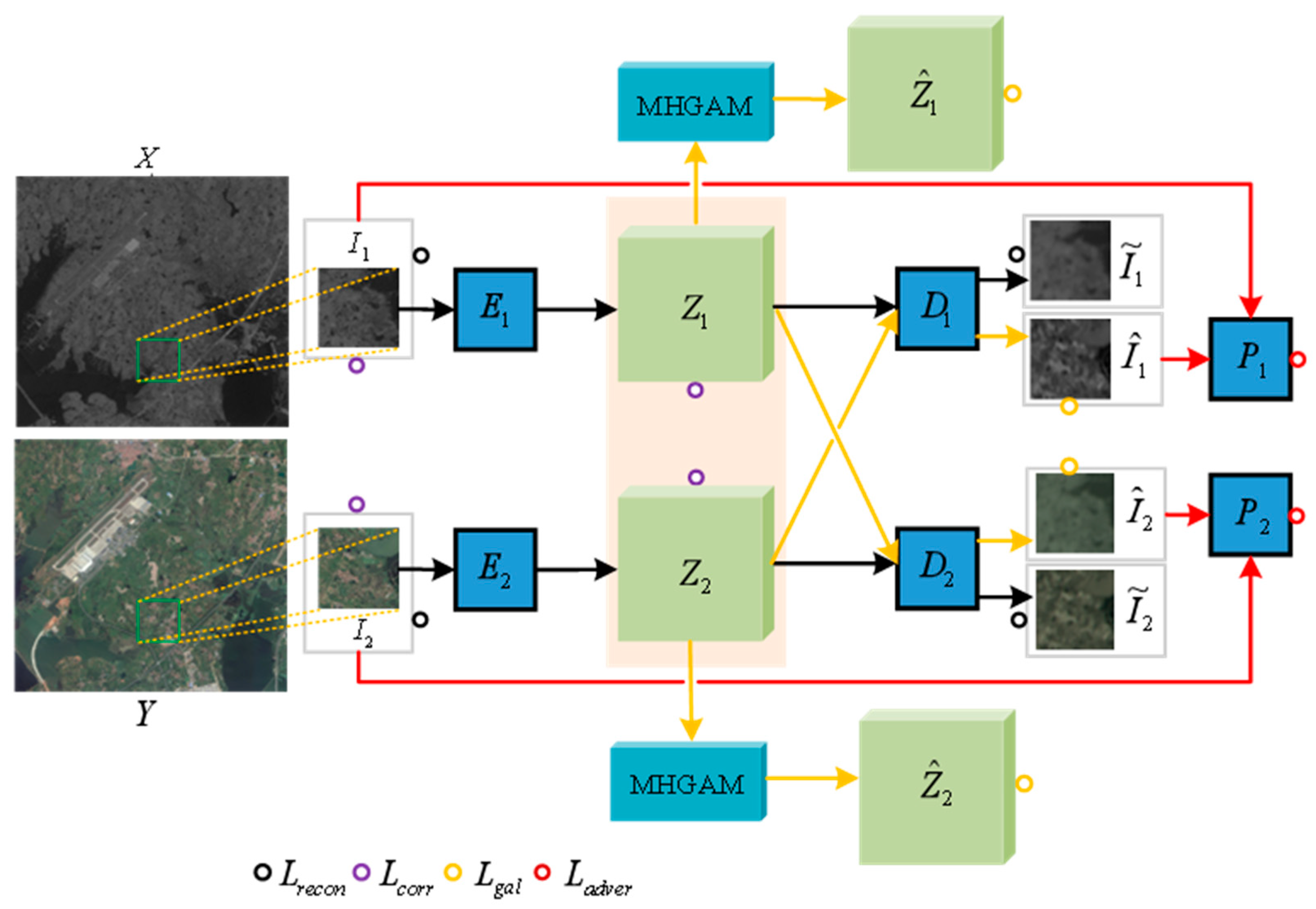
The overall architecture is shown in Figure 1, which realizes domain transformation and feature alignment of heterogeneous images through bidirectional mapping of encoder-decoder. The two encoder–decoder pairs are constructed using deep fully convolutional networks, where $Z_1$ and $Z_2$ represent the encoding layers or latent spaces of encoders $E_1$ and $E_{2,}$ respectively. $Z$ denotes the encoding layer representation of the tensors in $Z_1$ and $Z_2.$

With appropriate regularization, the bidirectional autoencoders can be jointly trained to learn the mapping of their inputs to the latent space domain. The latent features are then projected back into their original domains through the cascading of the encoder and corresponding decoder, producing high-fidelity reconstructions. Additionally, the data are mapped through the opposite decoder, which leads to the desired style transformation, as illustrated in Figure 2.

$$\widehat{Y}=F(X)=D_2(Z_1)=D_2(E_1(X))$$

(2)

$$\widehat{X}=G(Y)=D_1(Z_2)=D_1(E_2(Y))$$

(3)

However, without any external guidance, the feature representations of $\widehat{Y}$ and $X$, $\widehat{X}$ and $Y$ are typically not aligned, making it impossible to directly use them for generating difference maps. To address this, we introduce a loss term to enhance their transformation alignment. If the features of $\widehat{Y}$ and $X$, $\widehat{X}$ and $Y$ are successfully aligned, changes can be detected more accurately.

Specifically, the proposed MHGAN for heterogeneous remote sensing image change detection is based on two sets of autoencoder networks that fit the functions $F\left(\mathsf{\bullet }\right)$ and $G\left(\mathsf{\bullet }\right)$, respectively, to achieve domain transformation for dual-temporal remote sensing images. The training of the bidirectional autoencoders is carried out by minimizing a loss function with respect to the parameter $\upsilon$ of the constructed network. The loss function $L\left(\upsilon \right)$ consists of four components: reconstruction loss, code correlation loss, graph attention loss, and adversarial loss.

3.2. Reconstruction Loss

The first regularization term in the objective function of the MHGAN is the reconstruction loss, which aims to ensure that the reconstructed output images obtained after encoding and decoding by the network are as close as possible to the input images. Therefore, the reconstruction loss term can be expressed as follows:

$$L_{recon}=M(X_1,{\tilde{X}}_1)+M(Y_2,{\tilde{Y}}_2)$$

(4)

where $M$ represents the mean squared error (MSE) used to measure the loss between the expected output and the reconstructed output. The MSE is defined as the average of the squared differences between corresponding pixels in the input and reconstructed images.

3.3. Code Correlation Loss

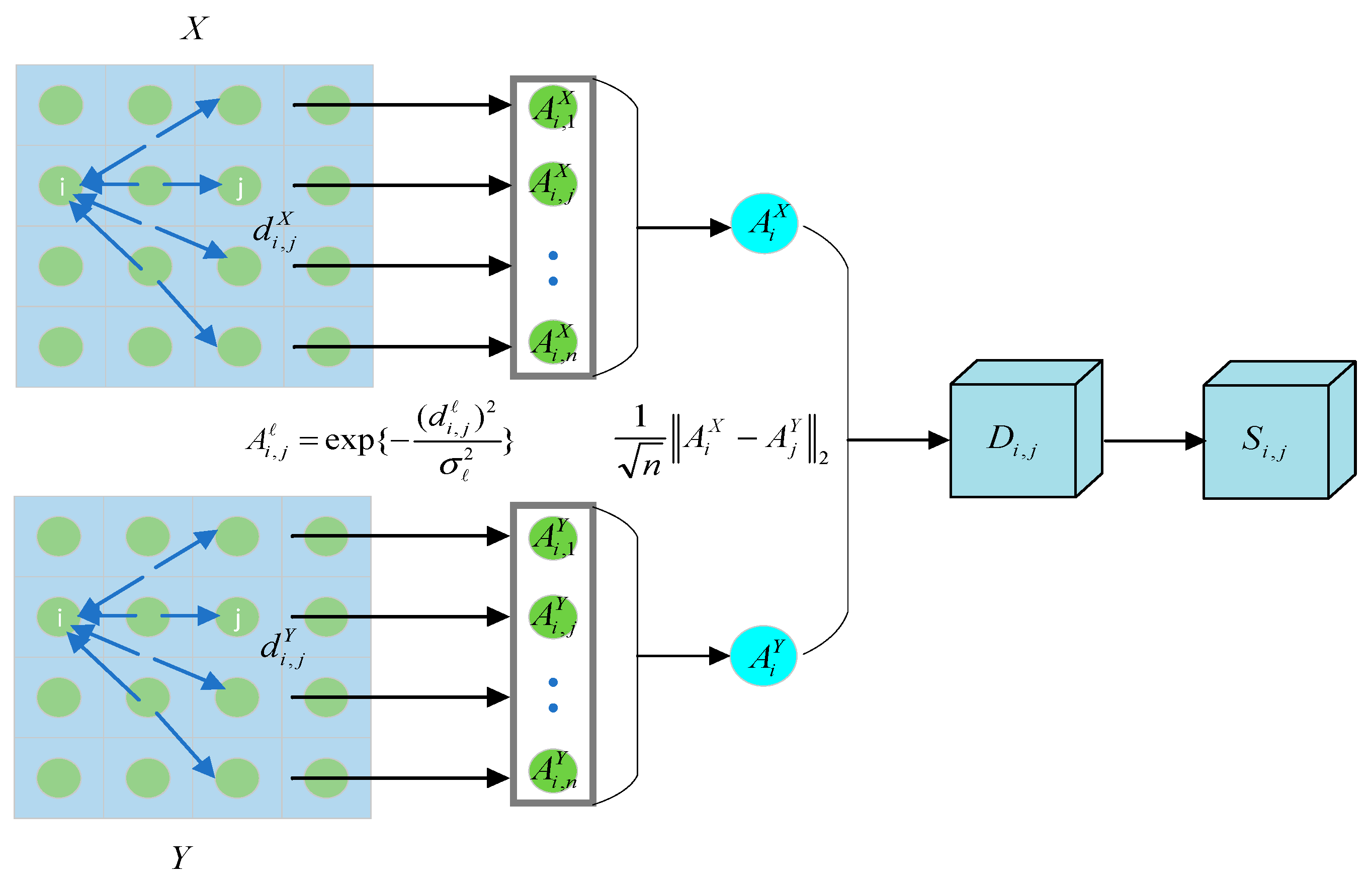
To align the feature representations of the encoding layer, a specific loss term known as the code correlation loss [2] has been introduced, as depicted in Figure 3. The objective is to synchronize the code layers of two autoencoders, treating them as a shared latent space. This allows the output of one encoder to serve as the input for both decoders, enabling the reconstruction of data within its native domain as well as its transformation into another domain. When pixel pairs $\left(i,j\right)$ are similar in the input space, their distances in the code space should also be close. Conversely, when pixel pairs $\left(i,j\right)$ are dissimilar in the input space, their distances in the code space should be more distant.

For any modality $X$ or $Y$, the feature distance for all pixel pairs $\left(i,j\right)$ within the same training patch is defined as

$$d_{i,j}^X=d^X(x_i,x_j),\hspace{1em}{d}_{i,j}^Y=d^Y(y_i,y_j)$$

(5)

where $x_i$ and $x_j$ are the feature vectors of the $i$-th and $j$-th pixels in patch $X$, respectively; $y_i$ and $y_j$ are the feature vectors of the $i$-th and $j$-th pixels in patch $Y$, respectively. $d^X$ and $d^Y$ are specific distance metrics, with Euclidean distance being the choice for this paper, formulated as

$$d^X(x_i,x_j)=\Vert x_i-x_j{\Vert }_2,\hspace{1em}{d}^Y(y_i,y_j)=\Vert y_i-y_j{\Vert }_2$$

(6)

Based on the aforementioned distance, the affinity matrix for local pixel pairs is calculated as follows:

$$A_{i,j}^x=exp\left(-{\displaystyle \frac{{\left(d_{i,j}^x\right)}^2}{s_i^2}}\right),\hspace{1em}{A}_{i,j}^y=exp\left(-{\displaystyle \frac{{\left(d_{i,j}^y\right)}^2}{s_i^2}}\right)$$

(7)

where $A_{i,j}^x \mathrm{a}\mathrm{n}\mathrm{d} { A}_{i,j}^y\in \left[\mathrm{0,1}\right]$ represent the similarity between pixel pairs (with values closer to 1 indicating higher similarity). The Gaussian kernel function smoothly maps distances in the feature space to similarity scores, enhancing robustness against noise. ${\sigma }_i$ is the kernel width, and in CAA, ${\sigma }_i$ is set as a fixed value, typically the mean distance of the $k$-nearest neighbors. However, determining kernel width in this manner depends on the ranked distances of neighboring points (e.g., the closest 25% of data points) and does not explicitly account for the density distribution of the entire image. Since data often exhibit varying densities across different regions, using a fixed kernel width may lead to the following issues:

• High-density regions: If the kernel width is too large, local structural information may become blurred, making it difficult to capture fine details.
• Low-density regions: If the kernel width is too small, the kernel function may fail to adequately cover the data, resulting in insufficient information.

To address this issue, this study adopts a density estimation-based approach, where a dynamic kernel width is assigned to each pixel based on its local density. High-density regions are assigned smaller kernel widths, while low-density regions are assigned larger kernel widths, thereby better accommodating the non-uniform distribution of the data The local density $p\left(x_i\right)$ of each pixel $x_i$ is first calculated through kernel density estimation based on the surrounding pixels:

$$p(x_i)={\displaystyle \frac{1}{n}}{\displaystyle \sum _{j=1}^{n}exp}\left(-\Vert x_i-x_j{\Vert }^2\right)$$

(8)

where $n$ represents the total number of surrounding pixels, and $\parallel x_i-x_j\parallel$ denotes the Euclidean distance between pixel $x_i$ and pixel $x_j.$ The kernel width ${\sigma }_i$ is then calculated as the inverse of the local density:

$${\sigma }_i={\displaystyle \frac{\xi }{p(x_i)}}$$

(9)

where $\xi$ is a tuning parameter determined via cross-validation on the training subsets of all four datasets. It controls the sensitivity of kernel width to local density: smaller values of $\xi$ (e.g., 0.1) make kernel width more responsive to density variations, while larger values (e.g., 0.5) produce a smoother effect. Based on validation results, the selected value of $\xi$ achieves a balance between capturing fine local details in high-density regions and ensuring robustness to noise in low-density areas.

The affinity calculation used in this study is better adapted to the local characteristics of the data distribution. High-density regions capture finer local differences, while low-density regions mitigate the effects of excessive noise amplification. Compared to fixed kernel widths, dynamic kernel widths can more effectively reflect both local and global variations within the image. This method is particularly suitable for scenarios where significant distribution differences exist between modalities, such as SAR and optical imagery, infrared and multispectral imagery, etc.

Each row of the affinity matrix is considered as the feature representation of a pixel:

$$A_i^X=\left[\begin{array}{c}{A}_{i,1}^X,A_{i,2}^X,\dots ,A_{i,n}^X\end{array}\right],\hspace{1em}{A}_j^Y=\left[\begin{array}{c}{A}_{j,1}^Y,A_{j,2}^Y,\dots ,A_{j,n}^Y\end{array}\right]$$

(10)

where $A_i^X$ is a vector that encompasses the similarity values of pixel $i$ with all other pixels in modality $X$. Similarly, $A_j^Y$ contains the similarity values of pixel $j$ with all other pixels in modality $Y$. By calculating the cross-modal distance, the following distance in the cross-modal space is obtained:

$$D_{i,j}={\displaystyle \frac{1}{\sqrt{n}}}\Vert A_i^X-A_j^Y{\Vert }_2$$

(11)

where $D_{i,j}\in \left(\mathrm{0,1}\right]$, representing the normalized distance that indicates the degree of similarity between pixels across modalities. The essence of this formula is that if two pixels exhibit similar patterns of similarity with other pixels in different modalities (i.e., their similarity vectors are alike), then the cross-modal distance between these two pixels should be small. Conversely, if there is a significant difference in the similarity vectors, the cross-modal distance will be larger. By representing each pixel with its affinity vector relative to other pixels, a relational feature is formed for each pixel. These relational features reflect the distribution characteristics of pixels within the local context. The features of a single pixel may not be sufficient to capture global or local changes, but by considering its relationships (affinity) with other pixels, a more comprehensive description of the structural information between pixels can be provided. These relational features are well suited for transfer to cross-modal alignment tasks.

To ensure that the similarity in the input space is maintained in the encoding layer, a similarity matrix $S_{i,j}$ is defined as follows:

$$S_{i,j}=1-D_{i,j}$$

(12)

As Figure 3 illustrated, $S_{i,j}\in \left[\mathrm{0,1}\right]$. The encodings in the encoding layer are denoted as $z_i^X$ and $z_j^Y$, corresponding to the encodings of pixel $i$ in modality $X$ and pixel $j$ in modality $Y$, respectively. By optimizing the encoding alignment loss, the similarity between $z_i^X$ and $z_j^Y$ is constrained to be consistent with $S_{i,j}.$

$$R_{i,j}={\displaystyle \frac{{(z_i^X)}^T{z}_j^Y}{‖z_i^X‖·‖z_j^Y‖}}$$

(13)

where $R_{i,j}\in \left[-\mathrm{1,1}\right],$ representing the cosine similarity between the encodings, with the goal of making $R_{i,j}\approx S_{i,j}$. The cosine similarity $R_{i,j}$ between pixel pairs in the encoding space serves as a representation of similarity at the encoding layer.

Ultimately, the similarity $R_{i,j}$ between pixel pairs in the encoding space is enforced to be consistent with the similarity $S_{i,j}$ in the input space. The code correlation loss $L_{corr}$ is defined as

$$L_{corr}=\parallel R-S{\parallel }_F^2$$

(14)

where $R$ represents the similarity matrix of all pixel pairs in the encoding layer. $S$ denotes the similarity matrix of pixel pairs between the input images $X$ and $Y$. This loss function $L_{corr}$ is the expected value of the squared Frobenius norm of the difference between the similarity matrices $R$ and $S$, which encourages the encodings to preserve the input space similarities.

3.4. Graph Attention Loss

As illustrated in Figure 2, the methodology for data transformation employing a unidirectional convolutional autoencoder is outlined. For image $X$, a random image patch $I_1$ is selected and encoded into the latent space using encoder $E_1$. Subsequently, the decoder $D_2$, associated with image $Y$, is utilized to decode the features from the latent space, resulting in an image patch ${\widehat{I}}_2$ that mirrors the style of image $Y$. This transformation is mathematically expressed as ${\widehat{I}}_2=F\left(I_1\right)=D_2\left(E_1\left(I_1\right)\right)$. Analogously, for image $Y$, an image patch $I_2$ is randomly extracted and encoded using encoder $E_2$. Then, the decoder $D_1$, corresponding to image $X$, decodes the features to generate an image patch ${\widehat{I}}_1$ that aligns with the style of image $X$. This process is represented as ${\widehat{I}}_1=G\left(I_2\right)=D_1\left(E_2\left(I_2\right)\right)$. 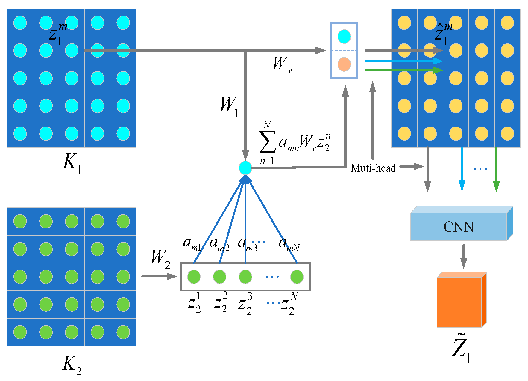To synchronize the image representations of ${\widehat{I}}_2$ with $I_1$ and ${\widehat{I}}_1$ with $I_2$, a novel structure based on the MHGAM is introduced, as shown in Figure 4.

This approach leverages the MHGAM to uncover latent spatial feature relationships within the spatial domain. It is independent of manual labeling and does not require specific prior knowledge. The assumption is that regions that remain unchanged can capture a greater degree of spatial correlation, thereby enhancing the effectiveness of feature representation.

Giving encoders $E_1$ and $E_2$ to obtain feature maps $Z_1$ and $Z_2$, respectively, these feature maps are then subjected to a linear transformation using a $1\times 1\times C$ convolutional kernel to derive node representations. This transformation results in the creation of a graph that represents the relationships between each node, where $C$ denotes the number of the feature channels. Let ${ V}_1$ represent the set of all nodes contained within $Z_1$ and $V_2$ represent the set of all nodes contained within $Z_2$. A bipartite graph is constructed to model the images’ before and after change for each pair $\left(m,n\right)\in E$, where $m\in V_1$ and $n\in V_2$, and the coefficient $e_{mn}$ signifies the correlation between nodes $m$ and $n$. The feature vectors $z_1^m\in$ ${\mathbb{R}}_1^c$ and $z_2^n\in$ ${\mathbb{R}}_2^c$ represent the nodes $m$ and $n$ in the latent space. The greater the similarity between the features of the images before and after change, the higher the likelihood that the region remains unchanged. Consequently, more spatial correction information should be conveyed to such regions. The correlation $e_{mn}$ is thus defined to be directly proportional to the similarity of the feature vectors of nodes $m$ and $n$. The inner product of the feature vectors is used to calculate this similarity:

$$e_{mn}={(W_1{z}_1^m)}^T(W_2{z}_2^n)$$

(15)

where $W_1\in {\mathbb{R}}_1^c$ and $W_2\in {\mathbb{R}}_2^c$ are linear transformations applied to each node in $Z_1$ and $Z_2$, respectively. They can also be interpreted as two weight matrices. This formula quantifies the correlation between nodes $m\in V_1$ and $n\in V_2$ using the inner product of linearly transformed feature vectors. From a technical mechanism perspective, the linear transformation (via weight matrices $W_1$, $W_2$) projects features into a shared subspace, enabling cross-domain comparison. The inner product then measures the similarity of these projected features, reflecting the spatial coupling strength between bitemporal features. A higher value indicates stronger similarity in structural characteristics (e.g., unchanged regions like stable terrain) as the mechanism effectively captures consistent spatial patterns across domains.

Based on the correlation coefficient $e_{mn}$, a self-attention mechanism is applied to the nodes. The influence of node $n$ on node $m$ is represented by $a_{mn}$, which is obtained by normalizing the correlation coefficient $e_{mn}$ using the SoftMax function:

$$a_{mn}={\displaystyle \frac{\exp (e_{mn})}{{\displaystyle {\sum }_{k\in V_2}\exp (e_{ik})}}}$$

(16)

where the SoftMax normalization ensures that attention weights $a_{mn}$ sum to 1, quantifying the proportion of information from node n, which propagates to node m. Technically, SoftMax operates by exponentiating and normalizing the similarity scores from Formula (15), which inherently prioritizes nodes with larger raw similarity values. This mechanism leverages the structural consistency encoded in the graph-nodes with stronger spatial correlations (e.g., adjacent pixels in unchanged urban areas) receiving higher weights, while noise-induced false correlations (from speckle or sensor artifacts) are suppressed due to their lower relative similarity.

The coefficient $a_{mn}$ determines the extent to which information from all nodes in $V_2$ is propagated to the $m$-th node in $V_1$. A linear transformation matrix $W_v\in {\mathbb{R}}_2^c$ is applied to the features of $V_2$, resulting in the aggregation of information for node $m$ as follows:

$$v_m={\displaystyle \sum _{n\in V_2}{a}_{mn}}{W}_v{z}_2^n$$

(17)

By integrating the aggregated representation $v_m$ with the node feature $z_1^m$, a more robust feature representation ${\widehat{z}}_1^m$ is obtained:

$${\widehat{z}}_1^m=ReLU\left(v_m\parallel \left(W_v{z}_1^m\right)\right)$$

(18)

where $\parallel$ denotes the vector concatenation operator. This attention mechanism functions as a unidirectional feed forward neural layer. The process is parallelized for all $z_1^m$, where $\forall m\in V_1$, resulting in a new feature map ${\widehat{Z}}_1$. Similarly, a new feature map ${\widehat{Z}}_2$ can be computed for image $Y$ using the same method. These formulas aggregate context-aware information from cross-domain nodes and fuse it with the original features. From a technical standpoint, the aggregation leverages the attention weights to selectively combine relevant cross-domain features. The fusion with original features balances new context acquisition and preservation of raw input information. This enhances the representation of consistent regions by reinforcing shared structural patterns while preserving discriminative features of changed regions (e.g., newly built roads) through retention of unique local characteristics, ultimately balancing stability and sensitivity to changes.

After this step, the feature maps ${\widehat{Z}}_1$ and ${\widehat{Z}}_2$ have been updated once. However, in the context of CD in heterogeneous remote sensing images, the features of the images before and after change may differ significantly. A single update of the feature maps could potentially overlook important feature information. To address this, the MHGAM is designed to include additional attention heads. By repeating the process for each attention head $k$, and then concatenating the feature maps ${\widehat{Z}}_1$ obtained from each attention head, the final output ${\widehat{Z}}_1$ of the MHGAM is produced:

The aggregated feature representation ${\tilde{Z}}_1$ is calculated by summing the feature maps from each attention head and then taking their average:

$${\tilde{Z}}_1={\displaystyle \frac{1}{K}}\sum _{k=1}^K{\widehat{Z}}_1^k$$

(19)

where ${\tilde{Z}}_2$ is a pixel-level distance metric function. The number of attention heads $K$ was determined experimentally. We tested $K$ = 2, 4, and 8 and found that $K$ = 4 provides the optimal balance. Fewer heads (e.g., 2) fail to capture diverse feature relationships (e.g., both spectral and spatial correlations), while a larger number of heads (e.g., 8) increases computational cost without yielding significant performance improvements. In Equation (19), features from the $K$ heads are aggregated by averaging, effectively fusing complementary information from different subspaces (each head learns distinct spatial correlation patterns). This strategy avoids over-reliance on a single attention head and enhances the robustness of the feature representation. To meet computational cost constraints, the Euclidean distance is preferred.

$$L_{gal}=d_2\left({\widehat{I}}_1,{\tilde{Z}}_1\right)+d_2\left({\widehat{I}}_2,{\tilde{Z}}_2\right)$$

(20)

where $d_2\left(·\right)$ is a pixel-level distance metric function. To meet computational cost constraints, the Euclidean distance is preferred.

By utilizing the graph attention loss, a node matching relationship between feature images is established, which helps to reduce the impact of spectral feature differences between image pairs on the analysis of the target area. The MHGAM allows the model to learn features in different spaces. It processes input features in parallel using multiple independent attention heads, with each head capable of learning different feature representations and relationships, thereby enhancing the model’s expressive power. The MHGAM maps spatial information from one feature domain to another, resulting in more effective image embedding representations. This approach better handles the heterogeneity between cross-domain image pairs.

3.5. Adversarial Loss

The bidirectional autoencoder network functions as a generator that facilitates the transformation of heterogeneous data, producing images with improved stylistic consistency. However, images generated solely through convolutional autoencoder networks may fail to fully achieve the desired style transfer effects. To overcome this limitation, a discriminator is introduced to assess the stylistic consistency between the generated and original images, ensuring that the transferred style more closely matches the characteristics of the target image. By jointly training the generator and the discriminator, the goal of ideal style transfer can be gradually achieved. A straightforward approach involves feeding input data pairs $\left({\widehat{I}}_1,I_1\right)$ and $\left({\widehat{I}}_2,I_2\right)$ into the discriminator network. The discriminator distinguishes between the pixel distributions of the transformed images and the real images, constructing an adversarial loss function that compels the generated images to have more consistent styles. Mathematically, this can be expressed as

$$L_{adver}=\underset{F}{min}\underset{P_2}{ax }{L}_{GAN,1\to 2}+\underset{G}{min}\underset{P_1}{max }{L}_{GAN,2\to 1}$$

(21)

$$L_{GAN,1\to 2}={\mathbb{E}}_{I_2\sim P_{data\left(I_2\right)}}\left[log{P}_2\left(I_2\right)\right]+{\mathbb{E}}_{I_1\sim P_{data\left(I_1\right)}}\left[log{(1-P}_2\left({\widehat{I}}_2\right)\right)]$$

(22)

$$L_{GAN,2\to 1}={\mathbb{E}}_{I_1\sim P_{data\left(I_1\right)}}\left[log{P}_1\left(I_1\right)\right]+{\mathbb{E}}_{I_2\sim P_{data\left(I_2\right)}}\left[log{(1-P}_2\left({\widehat{I}}_1\right)\right)]$$

(23)

3.6. Total Loss

The total loss is defined as the weighted average of four loss terms, as shown below:

$$L_{total}=L_{recon}+\alpha L_{corr}+\beta L_{gal}+\gamma L_{adver}$$

(24)

where $\alpha ,\beta$, and $\gamma$ are hyperparameters used to balance the four loss terms.

Upon conclusion of the training regimen, the anticipated difference image $\Delta$ is constructed in accordance with Equation (1). Subsequently, the quintessential Otsu thresholding technique is harnessed to ascertain the definitive CD outcome, encapsulated within the change map. The crux of this threshold selection algorithm lies in the identification of the optimal threshold value. Once the ultimate threshold is established, it serves as the benchmark for evaluating all pixel values. Pixels exceeding this threshold are classified as exhibiting change, while those falling below are categorized as unaltered.

The determination of pixel classification within the change map $CM$ is mathematically formalized as follows:

$$CM=\left\{\begin{array}{cc}1,\hfill & if \Delta \ge threshold\hfill \\ 0,\hfill & else\hfill \end{array}\right.$$

(25)

4. Experimental Study

4.1. Experimental Settings and Datasets

The experimental validation of the proposed MHGAN network was carried out utilizing four distinct public heterogeneous remote sensing image datasets. Figure 5 shows the two-phase images of these four sets of datasets along with the variation reference plots:

• Italy Dataset [29]: Captured by Landsat-5 over Sardinia, this dataset measures 412 × 300 pixels. It includes a NIR band image from September 1995 and an RGB image from July 1996. The ground truth reflects the actual lake expansion in Sardinia.
• California Dataset [28]: This dataset, initially 3500 × 2000 pixels, was downsampled to 875 × 500 for training. It includes an RGB image from Landsat 8 on 5 January 2017, and a SAR image from Sentinel-1A on February 18, 2017. The true change map depicts the effects of flooding.
• Tianhe Dataset [34]: With dimensions of 666 × 615 pixels, this dataset covers an area of 7.28 × 6.73 km² with an approximate resolution of 11 m/pixel. It features a panchromatic image from Landsat-7 in July 2002 and an optical image from Google Earth in June 2013. The change map illustrates building alterations at Wuhan Tianhe Airport.
• Shuguang Dataset [29]: Measuring 593 × 921 pixels with an approximate resolution of 8 m/pixel, this dataset includes a C-band SAR images from Radarsat-2 in June 2008 and an optical image from Google Earth in September 2012. The change map reveals building expansion in Shuguang Village.

The architecture of the proposed MHGAN consists of two encoder–decoder pairs, forming the core components of the network. Each encoder comprises two convolutional layers with dimensions 3 × 3 × 50, utilizing LeakyReLU as the activation function. The subsequent convolutional layer adopts 3 × 3 × 3 dimensions with the Tanh activation function to generate latent feature representations of size 100 × 100 × 3. Decoders mirror this structure, with the final layer applying a 3 × 3 × C convolution and Tanh activation to reconstruct the features back into the original image dimensions. The negative slope coefficient for LeakyReLU is set to 0.3. The Tanh function normalizes data within the [−1,1] range, aiding the convergence process during training [39].

The network was implemented using TensorFlow, and all experiments were conducted on a personal computer equipped with an NVIDIA GeForce RTX 2080 Ti (11 GB VRAM) and 16 GB RAM, running a Windows 10 environment. For development, PyCharm Professional Edition 2022.1 was used as the primary integrated development environment. During training, the Adam optimizer was employed due to its adaptive learning rate capabilities, and the model’s parameters were updated using the minimum value of the learning decay strategy. The training process lasted 40 epochs, with the network receiving 100 × 100 random image patches at each epoch. To enhance robustness against adversarial examples, a continuous random cropping technique was employed, ensuring variability in image input. The batch size and learning rates were specifically tuned to values of 25, 100, 50, and 1, respectively.

4.2. Evaluation Criteria

To evaluate the performance of the proposed MHGAN, four quantitative assessment criteria are adopted via comparison of each binary change detection map with the ground truth map: false positives ($FP$), false negatives ($FN$), overall accuracy ($OA$), and Kappa coefficient ($Kappa$) [40]. Meanwhile, the area under the ROC curve (AUC) was utilized to evaluate the difference image.

$$OA={\displaystyle \frac{TP+TN}{FP+FN+TP+TN}}$$

(26)

where $TP$ (true positives) are correctly identified changes; $TN$ (true negatives) are correctly identified no-changes; $FP$ (False Positives) are no-changes incorrectly identified as changes; and $FN$ (False Negatives) are changes incorrectly identified as no-changes.

The Cohen Kappa coefficient ($Kappa\in \left[-\mathrm{1,1}\right]$) assesses the consistency between two classifiers. The value of 1 indicates perfect agreement, −1 indicates perfect disagreement, and 0 suggests no association (random guessing). The coefficient is computed as

$$kappa={\displaystyle \frac{p_o-p_e}{1-p_e}}$$

(27)

where $p_o$ is the observed agreement (equivalent to $OA$), and $p_e$ is the probability of random agreement, estimated based on $TP$, $TN$, $FP,$ and $FN$:

$$p_e={\displaystyle \frac{(TP+FP)·(TP+FN)}{(TP+TN+FP+FN{)}^2}}+{\displaystyle \frac{(FN+TN)·(FP+TN)}{(TP+TN+FP+FN{)}^2}}$$

(28)

The AUC is a measure of the model’s ability to distinguish between classes. It is derived from the Receiver Operating Characteristic (ROC) curve, which is plotted by varying the classification threshold and recording the corresponding false-positive rate ($FPR$) and true-positive rate $\left(TPR\right).$

$$TPR={\displaystyle \frac{TP}{TP+FN}}$$

(29)

$$FPR={\displaystyle \frac{FP}{FP+FN}}$$

(30)

4.3. Compared Methods

To validate the effectiveness of the proposed algorithm, seven widely used traditional and deep-learning-based heterogeneous remote sensing image change detection methods were selected as comparison algorithms. These seven methods are as follows:

• CAA (code-aligned autoencoders for unsupervised change detection in multimodal remote sensing images [34]): The CAA approach leverages the power of conditional adversarial networks to identify alterations in images. By training on the disparities between images acquired at distinct temporal instances, CAA effectively discerns changes and is particularly adept at managing heterogeneous data, which encompasses data from diverse sensor types.
• NPSG (Nonlocal Patch Similarity Graph [28]): NPSG employs a graph-based strategy that focuses on the structural comparison of image patches, as opposed to pixel-level analysis. This method enhances the precision of change detection, proving especially beneficial in regions with intricate textures where traditional pixel-based methods may falter.
• INLPG (Improved NonLocal Patch-based Graph [29]): The INLPG represents an advanced iteration of the NPSG, engineered by Yuli Sun and colleagues. It refines the nonlocal patch similarity graph to elevate the performance of change detection, offering superior handling of both homogeneous and heterogeneous remote sensing images.
• ACE (deep image translation with an affinity-based change prior [41]): ACE introduces an unsupervised change detection technique grounded in adversarial cyclic encoding. Utilizing deep image translation methodologies, ACE incorporates an affinity-based change prior to bolster the accuracy of change detection across multimodal datasets, making it suitable for a range of optical and radar imagery.
• BASNet (Bipartite Adversarial Autoencoders with Structural Self-Similarity [42]): Based on the image transformation paradigm, a new bidirectional adversarial autoencoder network model is proposed for the change detection of unsupervised heterogeneous remote sensing images.
• IRGMcS (Iterative Robust Graph for Unsupervised Change Detection of Heterogeneous Remote Sensing Images [43]): IRGMcS proposes a robust graph mapping method for unsupervised heterogeneous change detection in remote sensing imagery. It leverages the shared structural information of the same ground objects across heterogeneous image pairs, addressing the challenge of directly comparing heterogeneous images due to differences in imaging mechanisms.
• TSCNet (Topological Structure Coupling Network for Change Detection of Heterogeneous Remote Sensing Images [35]): TSCNet leverages an encoder–decoder architecture to transform the feature space of heterogeneous images and incorporates wavelet transform, as well as channel and spatial attention mechanisms, to enhance the detection performance.

4.4. Results on Italy Dataset

Experiments were conducted on the Italy dataset using the proposed method and seven comparison algorithms. The experimental results are quantitatively described and compared using the evaluation metrics mentioned earlier, with visual comparison also provided. Figure 6 presents the final change maps obtained by the eight methods on the Italy dataset, while

Table 1. Results of change detection on Italy dataset.

Method	AUC	OA	Kappa	FP	FN
CAA	0.9008	0.9304	0.5167	6288	2313
NPSG	0.8978	0.8165	0.2851	21,273	1408
INLPG	0.9486	0.9308	0.5520	3022	6999
ACE	0.8722	0.9168	0.5450	3470	6812
BASNet	0.9120	0.9275	0.5180	6931	2035
IRGMcS	0.8811	0.9714	0.6928	1323	2214
TSCNet	0.8765	0.9303	0.4595	5243	3376
MHGAN	0.9378	0.9756	0.7078	920	2779

Note: Bold fonts indicate the optimal results in each column.

provides the quantitative analysis results for this dataset.

The challenge in detecting changes on the Italy dataset lies in the different acquisition bands of the images and the rugged mountainous terrain. The drastic variations in mountain heights lead to color discrepancies in the images, causing pixels from areas that should remain unchanged to be erroneously detected as change areas, which results in higher false positives, as indicated by the green marks in the change map. As shown in Figure 6c, the NPSG method achieves the lowest overall accuracy (0.8165), misclassifying the center of the lake in Sardinia as a change area. A similar issue is observed with the INLPG method to a certain extent. The MHGAN method exhibits the lowest number of false positives, as shown in Table 1, with only 920 false positives, demonstrating its advantage in suppressing background noise compared to the other methods. False negatives $\left(FN\right)$, which refer to detecting changed areas as unchanged, are mainly observed at the boundary between lakes and mountains, where the lake has expanded. The MHGAN method is positioned in the middle range among the eight methods, but upon comprehensive analysis, it is found to have the lowest number of incorrectly detected pixels ($FP$ + $FN$), indicating fewer background noise points while maintaining a strong ability to detect true change areas. This balance between false positives and false negatives allows the MHGAN to achieve the best performance of Kappa with an accuracy of 0.7078.

Figure 7 presents a visual demonstration of the MHGAN applied to the Italy dataset. It is evident that the input images undergo a transformation from one domain to another while maintaining a high degree of stylistic similarity to their original counterparts. Consequently, the enhancement in the effectiveness of change detection is pronounced.

Additionally, Figure 8 shows the ROC curves of the difference images for eight methods on the Italy dataset, with the corresponding AUC values provided in Table 1. It can be observed that the AUC value of the proposed method is higher than that of BASNet. Moreover, the proposed MHGAN method achieves the highest $OA$ and $Kappa$ results among the eight methods, demonstrating a significant improvement over the comparison methods.

4.5. Results on California Dataset

The change maps produced by the MHGAN and its comparison methods for the California dataset are illustrated in Figure 9. A notable challenge in detecting changes within this dataset arises from the flat terrain where the flooding occurred. While the widening of the main river channel caused by the flood is relatively straightforward to identify, the accurate detection of scattered small lakes and puddles around the river channel presents a greater difficulty. This challenge is evident in the change maps, where capturing the patchy and dispersed changes in the reference map proves to be a complex task.

In general, when comparison methods are applied to non-interactive regions, their performance often shows substantial variability in detecting large-scale or non-interactive changes. In contrast, the MHGAN method demonstrates strong capability in accurately identifying areas of river channel widening induced by flooding. According to

Table 2. Results of change detection on California dataset.

Method	AUC	OA	Kappa	FP	FN
CAA	0.9170	0.9137	0.5101	24,906	12,785
NPSG	0.7491	0.8444	0.1484	85,543	8194
INLPG	0.9268	0.9263	0.5188	16,136	16,100
ACE	0.8503	0.9119	0.4124	27,898	10,663
BASNet	0.9254	0.9071	0.4913	28,112	12,549
IRGMcS	0.9178	0.9279	0.4952	6646	24,906
TSCNet	0.8903	0.8886	0.4323	35,735	13,023
MHGAN	0.9235	0.9304	0.5438	17,210	14,389

Note: Bold fonts indicate the optimal results in each column.

, the MHGAN attains the highest $OA$ and Kappa, highlighting its outstanding overall performance and effectiveness in this scenario.

Figure 9 presents a visualization of the MHGAN on the California dataset. From Figure 10b,c, as well as Figure 10f,g, it can be observed that the style similarity between the transformed and original images is high, with unchanged regions remaining largely unaffected. This minimizes the impact of unchanged regions on CD results to the greatest extent.

The MHGAN trailing by only 0.03 percentage points. The other methods show a significant gap compared to them. Finally, the ROC curves of all comparison methods are shown in Figure 11. Among them, the ROC curve of the INLPG is the closest to the (0, 1) point, corresponding to the highest AUC value. Although the ROC curve of the MHGAN is inferior to that of the INLPG, the MHGAN achieves the best performance among all methods in suppressing background noise. Based on the above observations, the MHGAN ranks first in $OA$ and $Kappa$ indicating that it strikes a good balance between suppressing background noise and detecting change areas.

4.6. Results on Tianhe Dataset

Figure 12 shows the change maps generated by the MHGAN method and the comparison algorithms on the Tianhe dataset. The main changes in the Tianhe dataset involve the construction of two new buildings and a road. The difficulty in detecting these changes lies in the fact that the two new buildings were built at the ends of existing structures, making it easy to mistakenly classify parts of the old buildings as changes during detection. Additionally, the style differences introduced by the heterogeneous images further complicate the precise detection of change areas. These challenges are evident in the results for ACE and CAA, as shown in Figure 12.

While CAA correctly identifies the two new buildings, it also incorrectly labels the old building in the middle as a change area. Both methods also misclassify many unchanged areas around the new buildings as changed. Compared to CAA and ACE, the other methods perform better on the Tianhe dataset, accurately detecting the new buildings and road while avoiding numerous misclassifications of unchanged areas. Among these, the MHGAN produces the best results, accurately detecting both new buildings and the road without being affected by background noise or misclassifying other areas as changes. Additionally, in Figure 13, we present a visual example of the transformations obtained with the proposed method on the dataset used in this section. The evaluation results provided in

Table 3. Results of change detection on Tianhe dataset.

Method	AUC	OA	Kappa	FP	FN
CAA	0.9892	0.9159	0.1999	34,260	135
NPSG	0.9936	0.9938	0.7314	1202	1331
INLPG	0.9975	0.9920	0.7143	545	2720
ACE	0.9783	0.9283	0.2166	29,099	261
BASNet	0.9913	0.9941	0.7420	1287	1148
IRGMcS	0.9469	0.9793	0.4952	8068	406
TSCNet	0.9956	0.9925	0.7121	2177	869
MHGAN	0.9972	0.9970	0.7787	1170	930

Note: Bold fonts indicate the optimal results in each column.

further support the analysis of the change maps. The INLPG achieves a slightly higher AUC (0.9975 vs. 0.9972) possibly due to its strength in capturing local structural similarities via nonlocal patch graphs. However, the MHGAN outperforms the INLPG in Kappa (0.7787 vs. 0.7143) because the multi-head graph attention mechanism better preserves global spatial relationships across domains, reducing misalignment-induced errors in large-scale unchanged regions. The MHGAN shows the fewest false positives (FN + FP), yielding the highest AUC of 0.9970 and the highest Kappa value of 0.7787.

Figure 14 illustrates the ROC curves for all methods. It is evident that the curves of all eight methods are closely aligned with the ideal point, with the curves of the MHGAN and INLPG being nearly indistinguishable. This observation is further supported by the AUC values in Table 3, where the INLPG achieves the highest AUC among all methods, with the MHGAN trailing by only 0.03 percentage points. The other methods show a significant gap compared to them.

4.7. Results on Shuguang Dataset

Figure 15 displays the change maps obtained by all methods on the Shuguang dataset. The main changes in the Shuguang dataset include the construction of a new building in the agricultural area at the top left, as well as a linear change region at the bottom right caused by terrain variations. The difficulty in detecting changes in this dataset arises from the presence of several narrow agricultural fields in the upper-right part of the new building, which remain unchanged. These fields are susceptible to seasonal effects and the heterogeneity of the image data, making them prone to being mistakenly classified as changed areas. Furthermore, the narrow linear region at the bottom right is prone to being affected by background noise, leading to its misclassification as unchanged.

Upon comparing the results in Figure 15, it is evident that the methods CAA, NPSG, INLPG, ACE, and IRGMcS all incorrectly classify the agricultural area next to the building as a change zone. In contrast, the proposed MHGAN method accurately identifies this region as unchanged. This is further supported by the results in

Table 4. Results of change detection on Shuguang dataset.

Method	AUC	OA	Kappa	FP	FN
CAA	0.8762	0.9586	0.6397	13,241	3699
NPSG	0.9657	0.9551	0.6388	23,304	1235
INLPG	0.9477	0.9733	0.6744	8997	5587
ACE	0.9679	0.9508	0.5763	4870	22,024
BASNet	0.9242	0.9775	0.6870	1368	10,909
IRGMcS	0.8834	0.9825	0.7935	3889	5667
TSCNet	0.9571	0.9696	0.4955	26	16,558
MHGAN	0.9183	0.9895	0.8245	1645	4634

Note: Bold fonts indicate the optimal results in each column.

, which show that the MHGAN has the lowest number of false positives ($FP$ + $FN$), indicating its superior ability to suppress background noise. As a result, the MHGAN achieves the highest $OA$ of 0.9895, demonstrating its effective suppression of background noise while accurately detecting changed areas. Moreover, the highest Kappa value of 0.8245 indicates that the MHGAN maintains a good balance between detecting both the background and the changed areas. The MHGAN’s lower AUC compared to ACE in Shuguang dataset is due to their differing design goals. ACE uses an affinity-based change prior [41] that amplifies local differences, which boosts AUC but increases false positives (e.g., mistaking speckle noise in bare soil for changes). In contrast, the MHGAN’s graph attention loss suppresses noise in homogeneous regions (e.g., agricultural fields) by emphasizing structural consistency, reducing false alarms but slightly lowering AUC. This discrepancy reflects the MHGAN’s focus on reliable change maps with minimal false detections, which is more valuable in applications like land use monitoring where precision is critical. The MHGAN prioritizes suppressing false positives, making it more reliable for practical applications where reducing false alarms is critical. Figure 16 showcases a visual representation of the MHGAN when applied to the Shuguang dataset. Upon examination of Figure 16b,c, as well as Figure 16f,g, it is evident that the transformed images exhibit a high degree of stylistic similarity to their original images. The consistency in unaltered regions is particularly notable, which significantly mitigates the impact of these regions on the CD outcomes, thereby enhancing the accuracy of the CD process.

Figure 17 presents the ROC curves reflecting the classification performance of the network. Based on the corresponding AUC values, the results obtained by the MHGAN method are relatively modest. It can be observed that the curves of all eight methods are close to the ideal (0, 1) point, with NPSG and ACE showing the best performance. This is further confirmed by the AUC values in Table 4, where the ACE method achieves the highest AUC.

4.8. Ablation Study

To validate the effectiveness of the loss terms in optimizing and constraining network training, this section designs a series of ablation experiments for comparative analysis.

(1) Component Analysis. In these experiments, the network using only the reconstruction loss is considered the Baseline model. The other three loss terms are gradually added to the baseline model to construct the ablation models: Model-1 is Baseline + code correlation loss, Model-2 is Baseline + code correlation loss + adversarial loss, and the MHGAN is Baseline + code correlation loss + adversarial loss + graph attention loss. To facilitate direct performance comparison among these models, the CD results on four datasets are presented.

The performance of the models on the four datasets is evaluated using five overall metrics: AUC, $OA$, Kappa, $FP,$ and $FN$, with the results summarized in

Table 5. Change detection results of ablation models on Italy dataset.

Method	AUC	OA	Kappa	FP	FN
Baseline	0.2735	0.3002	−0.0584	81,705	4795
Model-1	0.8841	0.9040	0.4372	12,401	1578
Model-2	0.9164	0.9651	0.6105	12,447	2345
MHGAN	0.9378	0.9756	0.7078	920	2779

Note: Bold fonts indicate the optimal results in each column.

,

Table 6. Change detection results of ablation models on California dataset.

Method	AUC	OA	Kappa	FP	FN
Baseline	0.3289	0.2810	−0.0580	295,534	19,019
Model-1	0.8993	0.9128	0.4694	21,993	16,125
Model-2	0.9117	0.9302	0.5084	12,344	18,184
MHGAN	0.9235	0.9304	0.5438	17,210	14,389

Note: Bold fonts indicate the optimal results in each column.

,

Table 7. Change detection results of ablation models on Tianhe dataset.

Method	AUC	OA	Kappa	FP	FN
Baseline	0.8042	0.3155	0.0064	279,800	547
Model-1	0.9819	0.9907	0.6120	2059	1337
Model-2	0.9902	0.9929	0.6808	1338	1562
MHGAN	0.9972	0.9970	0.7787	1170	930

Note: Bold fonts indicate the optimal results in each column.

and

Table 8. Change detection results of ablation models on Shuguang dataset.

Method	AUC	OA	Kappa	FP	FN
Baseline	0.6075	0.1421	0.0061	467,437	1088
Model-1	0.9699	0.9704	0.5161	22	16,494
Model-2	0.9769	0.9712	0.7117	79	15,635
MHGAN	0.9183	0.9895	0.8245	1645	4634

Note: Bold fonts indicate the optimal results in each column.

. The change maps are shown in Figure 18. By incorporating code correlation loss, Model-1 achieves better alignment of feature representations, effectively mitigating the impact of interference from transformed data. As a result, Model-1 shows significant improvements in AUC, $OA$, and Kappa values across all four datasets compared to the Baseline model. With the addition of adversarial loss, Model-2 further enhances stylistic consistency in the common domain, making the generated pairs of images more consistent in style. Thus, Model-2 exhibits noticeable improvements over Model-1. Finally, with the inclusion of graph attention loss in the MHGAN, the model can more effectively transfer spatial information between feature domains, improving spatial alignment of feature representations and achieving domain transformation. Consequently, the MHGAN shows substantial improvements in AUC, $OA$, and Kappa values on the Italy and Tianhe dataset compared to Model-2. On the California dataset, the $OA$ value decreases slightly, but both AUC and Kappa show notable improvements. On the Shuguang dataset, the AUC value decreases somewhat, but the Kappa value increases significantly. Figure 19 illustrates the comparison of AUCs.

(2) Parameter Analyses. The total loss function introduced in this paper utilizes the parameters $\alpha ,\beta$, and $\gamma$ to balance the contributions of the four loss components. To evaluate the impact of these parameters on CD performance, a series of parameter combinations ($\alpha ,\beta$,$\gamma$) were tested, specifically (0.5, 0.5, 0.5), (2, 1, 1), (1, 2, 1), and (1, 1, 2). The four parameter combinations (0.5, 0.5, 0.5), (2, 1, 1), (1, 2, 1), and (1, 1, 2) were selected to systematically evaluate the influence of each loss component. Specifically, (0.5, 0.5, 0.5) serves as a baseline with equal weights across all losses. The other three combinations emphasize one loss term at a time: (2, 1, 1) highlights the code correlation loss, which is critical for cross-domain feature alignment; (1, 2, 1) emphasizes the graph attention loss, which models spatial relationships; and (1, 1, 2) focuses on the adversarial loss, which promotes style consistency. These values were chosen based on preliminary experiments, which indicated that the code correlation loss had the most significant impact on overall performance. Therefore, it was prioritized in our evaluation. The results, summarized in

Table 9. Results of change detection on the four datasets.

Datasets	$(\mathsf{\alpha },\mathsf{\beta },\mathsf{\gamma })$	AUC	OA	Kappa	FP	FN
Italy	(0.5, 0.5, 0.5)	0.9148	0.9043	0.4621	10,292	1535
	(2, 1, 1)	0.9378	0.9756	0.7078	920	2779
	(1, 2, 1)	0.9251	0.9442	0.6026	1782	1718
	(1, 1, 2)	0.9147	0.9467	0.5939	3888	2316
California	(0.5, 0.5, 0.5)	0.9045	0.9124	0.4441	20,342	17,976
	(2, 1, 1)	0.9235	0.9304	0.5438	17,210	14,389
	(1, 2, 1)	0.9117	0.9186	0.4764	18,727	17,059
	(1, 1, 2)	0.9249	0.9409	0.5155	14,040	16,205
Tianhe	(0.5, 0.5, 0.5)	0.9901	0.9848	0.5498	1777	3068
	(2, 1, 1)	0.9971	0.9971	0.7798	1175	927
	(1, 2, 1)	0.9892	0.9930	0.6824	1256	1594
	(1, 1, 2)	0.9909	0.9842	0.5397	5687	660
Shuguang	(0.5, 0.5, 0.5)	0.9526	0.9749	0.6158	381	13,580
	(2, 1, 1)	0.9183	0.9895	0.8245	1645	4634
	(1, 2, 1)	0.9761	0.9769	0.6625	468	12,122
	(1, 1, 2)	0.9472	0.9850	0.7094	2955	5195

Note: Bold fonts indicate the optimal results of various indicators on different datasets.

, show that when the parameters are set to (0.5, 0.5, 0.5), the performance of the MHGAN is suboptimal, indicating that reducing the influence of $L_{corr},{ L}_{gal}, \mathrm{a}\mathrm{n}\mathrm{d} L_{adver}$ leads to poorer CD outcomes.

In contrast, when the parameters are adjusted to (1, 2, 1) and (1, 1, 2), the MHGAN exhibits significant performance improvements compared to (0.5, 0.5, 0.5), demonstrating that increasing the weights of $L_{gal} and{ L}_{adver}$ positively impacts the model’s effectiveness. When the parameters are set to (2, 1, 1), the MHGAN achieves the best results across all four datasets. Thus, the final parameter values for $\alpha ,\beta$,$\gamma$ are set to (2, 1, 1).

4.9. Computational Resource Comparison

To evaluate computational efficiency, we compared the MHGAN with seven state-of-the-art methods on the same hardware (NVIDIA RTX 2080 Ti, 16 GB RAM).

Table 10. Computational resource comparison (average ± Std).

Method	Training Time (s/Dataset)	Inference Time (s/Image)	Peak Memory (GB)
CAA	430 ± 5	0.7 ± 0.1	7.2
NPSG	1147 ± 10	0.6 ± 0.1	4.5
INLPG	295 ± 4	0.6 ± 0.1	5.1
ACE	351 ± 4	1.2 ± 0.2	10.2
BASNet	220 ± 6	0.9 ± 0.1	8.0
IRGMcS	250 ± 7	1.0 ± 0.2	10.1
TSCNet	310 ± 7	0.8 ± 0.1	8.3
MHGAN	210 ± 5	0.8 ± 0.1	8.5

Note: Bold fonts indicate the optimal results in each column.

summarizes the average training time, inference time per image, and peak memory usage on four datasets.

The MHGAN achieves favorable computational resource consumption performance through a series of well-designed architectural choices. For training time (≈210 s/dataset), it benefits from the MHGAM, where a multi-head structure (four heads, optimized via ablation) enables parallelizable feature aggregation; this graph-based, localized attention reduces redundant computations, unlike methods with sequential or fully connected attention (such as NPSG’s non-local patch graph that incurs high pairwise comparison costs). Additionally, the bilateral adversarial framework, using a weighted combination of reconstruction, code correlation, and graph attention losses, avoids overfitting to noise (a common cause of prolonged training in methods like ACE that prioritize high sensitivity), thus converging faster on representative features. In terms of inference time (≈0.8 s/image), efficiency comes from the MHGAM’s pre-computed graph structures that minimize runtime graph construction, contrasting with methods like the INLPG that dynamically recompute non-local relationships per image and add latency and the encoder–decoder architecture, which compresses input features into a low-dimensional latent space feature maps in the bottleneck, reducing the computational load for change detection and outperforming uncompressed or weakly compressed methods (e.g., BASNet, which retains higher-resolution intermediate features). For peak memory (≈8.5 GB), memory efficiency is attained through the MHGAM constructing sparse graphs (retaining only top-k nearest neighbors per node) instead of dense cross-domain matrices, reducing memory overhead compared to methods like TSCNet that store full pairwise similarity matrices and the density-based dynamic kernel in the code correlation loss that avoids allocating fixed-size memory buffers for kernel operations, unlike methods with static kernels, as this adaptivity optimizes memory usage per-image based on local feature density.

5. Conclusions

This paper proposes an unsupervised change detection method for heterogeneous remote sensing images based on a MHGAN. The MHGAN employs four loss functions to facilitate unsupervised learning: reconstruction loss, code correlation loss, graph attention loss, and adversarial loss. To align feature representations in the encoding layer, a code correlation loss is introduced, enhanced by a density-based kernel width estimation method to better capture both local and global changes in heterogeneous images. To effectively transfer spatial information across feature domains and improve spatial alignment, a graph attention loss is designed. This loss models the relationship between features and images, enhances the representation of consistent regions in bitemporal images, and mitigates the impact of changes on the learning objectives. Additionally, an adversarial loss is incorporated to further promote style consistency within the shared domain, encouraging the network to generate paired images with homogeneous data structures and styles. Comparative experiments with state-of-the-art models demonstrate the superior performance of the MHGAN across four benchmark datasets for change detection tasks.