
Cascaded Detection Method for Ship Targets Using High-Frequency Surface Wave Radar in the Time–Frequency Domain

 , , , , and
Abstract

1. Introduction
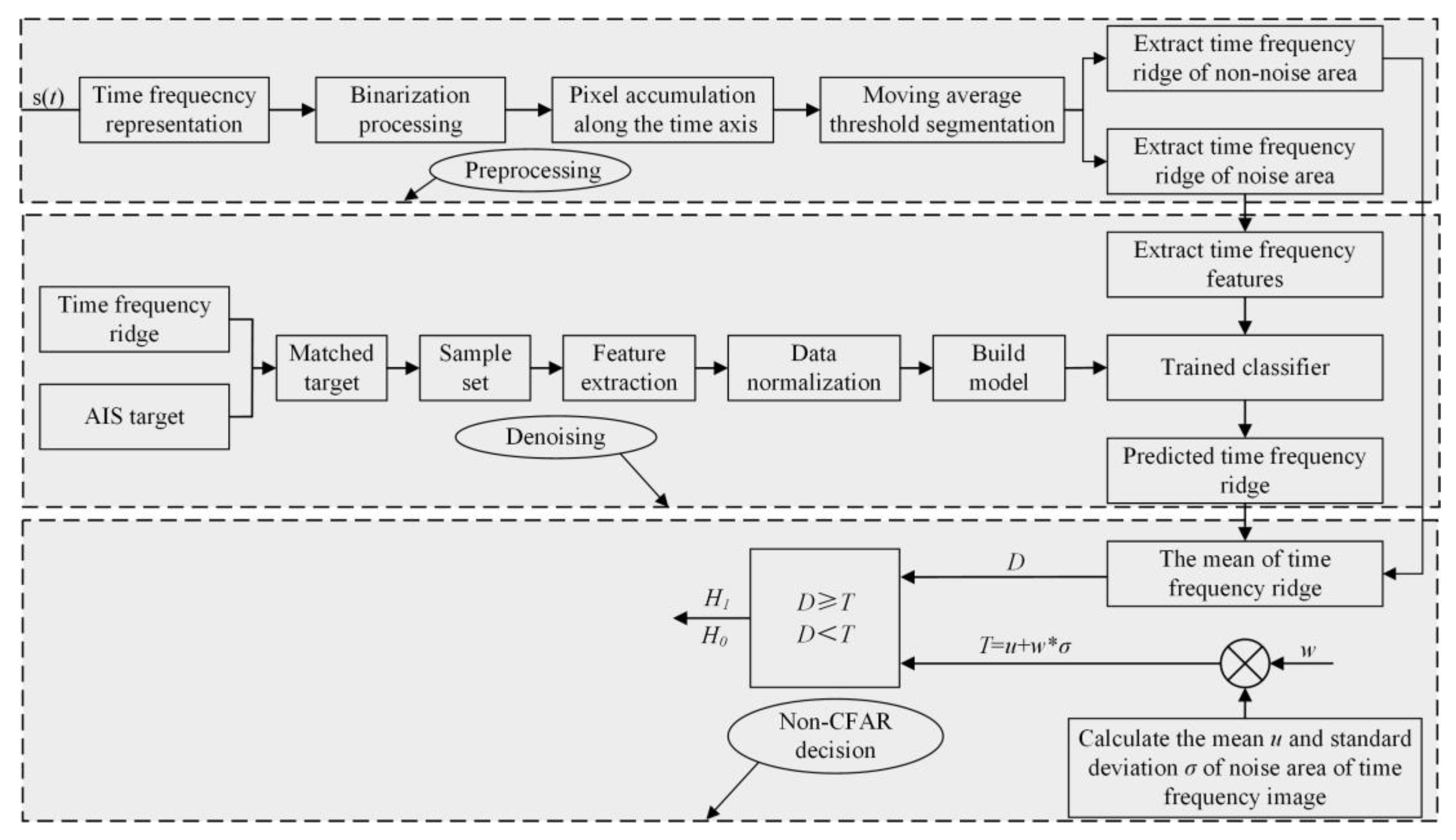
2. Methods
2.1. Theoretical Foundations
- (1)
- Mean absolute value: in radar target detection, the average amplitude of the echo signal serves as a primary indicator of target signal strength.N is the length of the TF ridge, which is equal to 256.
- (2)
- Aspect ratio: due to fluctuations in the ship’s RCS and observation angle, the TF ridge may appear continuous or intermittent. Additionally, differing radial velocities between the ship and noise cause their energy distributions to occupy separate Doppler frequency bands on the TF plane. Accordingly, the TF ridge aspect ratio is defined to capture this distinguishing characteristic. Let N denote the length of the extracted TF ridge, and W represent the number of Doppler distribution units. The TF ridge aspect ratio can then be expressed as
- (3)
- Kurtosis: kurtosis characterizes the sharpness of the data distribution along the TF ridge [35]. For a normal distribution, the kurtosis value is equal to 3. A high kurtosis indicates a peaked distribution, while a low kurtosis suggests a flatter profile.In Equation (4), mT represents the mean of Ridge(i), and σT represents the standard deviation of Ridge(i).
- (4)
- Skewness: skewness quantifies the asymmetry of the TF ridge amplitude distribution [36], and its calculation formula is as follows.
- (5)
- Variance: variance reflects the degree of signal energy dispersion, providing a means to distinguish target, clutter, and noise, as shown in the following equation.
- (6)
- Average amplitude change: the average amplitude change is computed as the mean of adjacent-point amplitude differences along the TF ridge, reflecting signal complexity.
- (7)
- Peak factor: the peak factor, defined as the ratio of the peak amplitude to the RMS value, indicates the presence of impulsive components in the signal. The calculation formula is as follows:max(·) represents taking the maximum value.
- (8)
- Ratio of standard deviations after bisection: the standard deviation of the entire TF ridge, denoted as std1, is first computed. The ridge is then bisected, and the standard deviation of one half, denoted as std2, is calculated. The ratio of the standard deviations is as follows:
- (9)
- Ratio of bisected means: the TF ridge coefficients are split into two groups based on the global mean. The means of the upper and lower subsets are denoted as m22 and m21, respectively. The ratio between the two is as follows:
- (10)
- Absolute standard deviation of the difference: this metric resembles the root mean square but is derived from the standard deviation of differences between adjacent TF amplitudes. Its calculation formula is as follows:
- (11)
- Integral ratio: the integral value represents the total energy of the TF ridge. The integral ratio compares this energy to that of the surrounding TF region, excluding the ridge. The formula is as follows:In Equation (12), t represents the duration of the TF ridge, and F represents the set of Doppler bins in the TF region. In the TF plane, noise exhibits a short duration and weak energy distribution, appearing scattered. However, the target signal can be approximated as a single-frequency signal with high TF concentration. Assuming that the TF region where the TF ridge of the target signal is located is represented by S(t, f), the TF amplitude distribution within this region can reflect the energy concentration of the TF ridge. Next, TF features are extracted from the TF region where the TF ridge is located.
- (12)
- Maximum kurtosis: kurtosis, which represents the normalized fourth-order central moment, characterizes the amplitude distribution within the TF region that encompasses the ridge [37]. It is commonly employed to determine whether a random variable follows a normal distribution.
- (13)
- Renyi entropy: Renyi entropy generalizes Shannon entropy and quantifies the TF energy concentration of the target signal for a given order α [38]. The value of Rα indicates the quality of TF concentration: a smaller Rα suggests better TF concentration, while a larger Rα indicates poorer TF concentration, with α set to 2 in this case.
- (14)
- Normalized third-order Renyi entropy [39].
- (15)
- Gradient: in the TF domain, the radar echo is represented as a 2D image, denoted as z = S(t, f). Assuming that z has continuous first-order partial derivatives within S, the gradient at each point (t, f) can be calculated using the following formula.The gradient of each pixel is calculated and accumulated sequentially, and the average gradient feature is obtained by averaging.
- (16)
- Image entropy: image entropy quantifies signal uncertainty, with higher entropy indicating greater randomness or complexity in the TF image. The formula for calculating image entropy is as follows.In Equation (17), k represents the grayscale level, ranging from 0 to 255, with K = 255, and pk denotes the probability of pixels at that level.
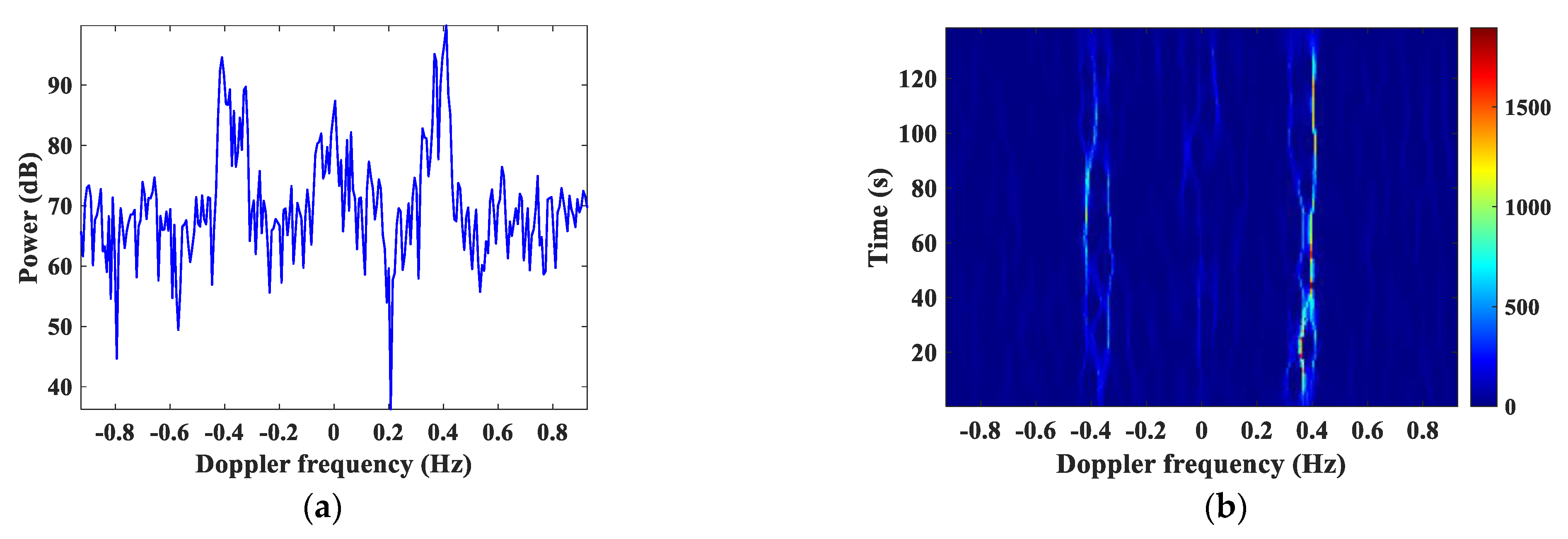
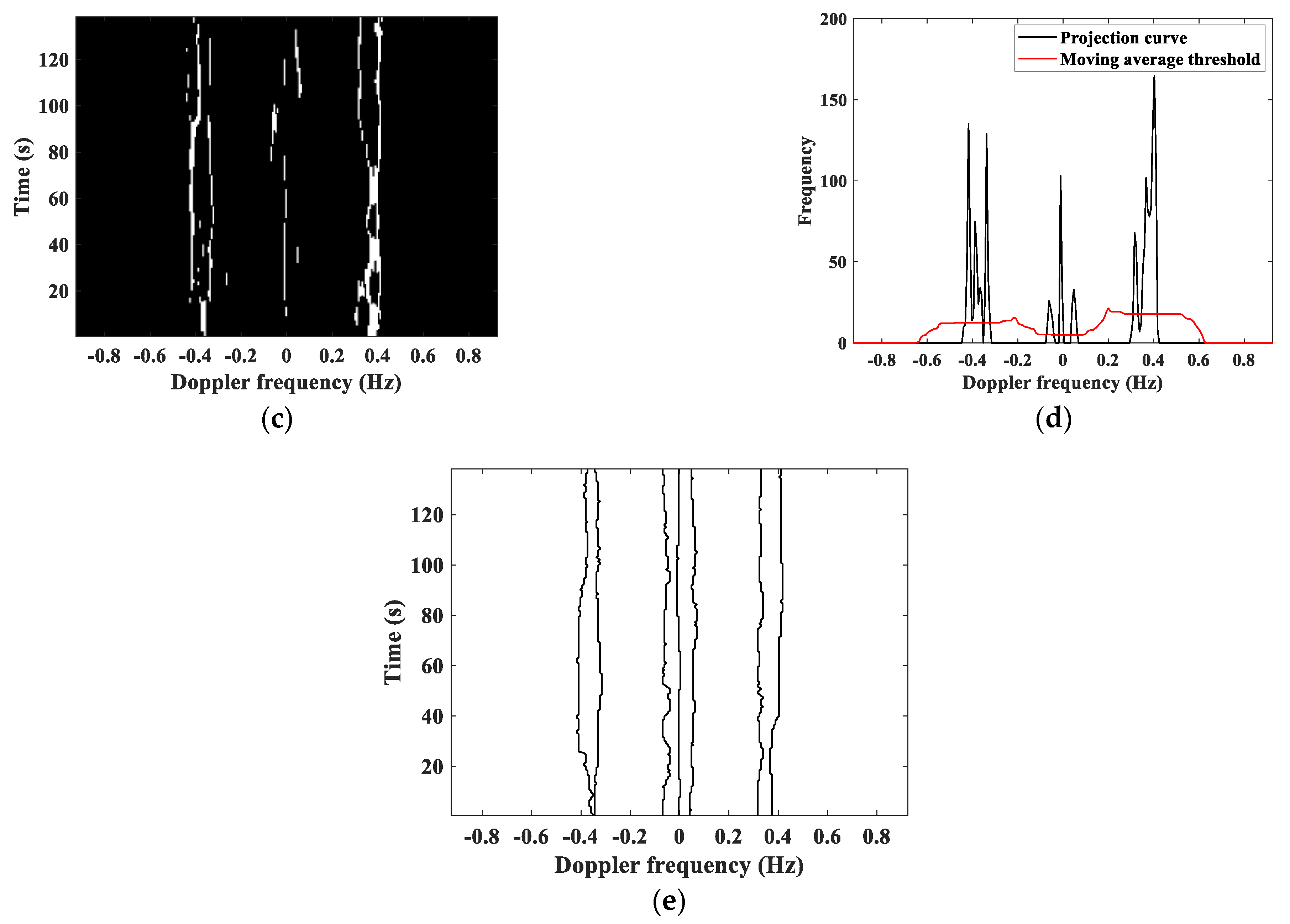
2.2. TF Ridge Extraction Method
2.3. Cascade Detection Method
3. Results
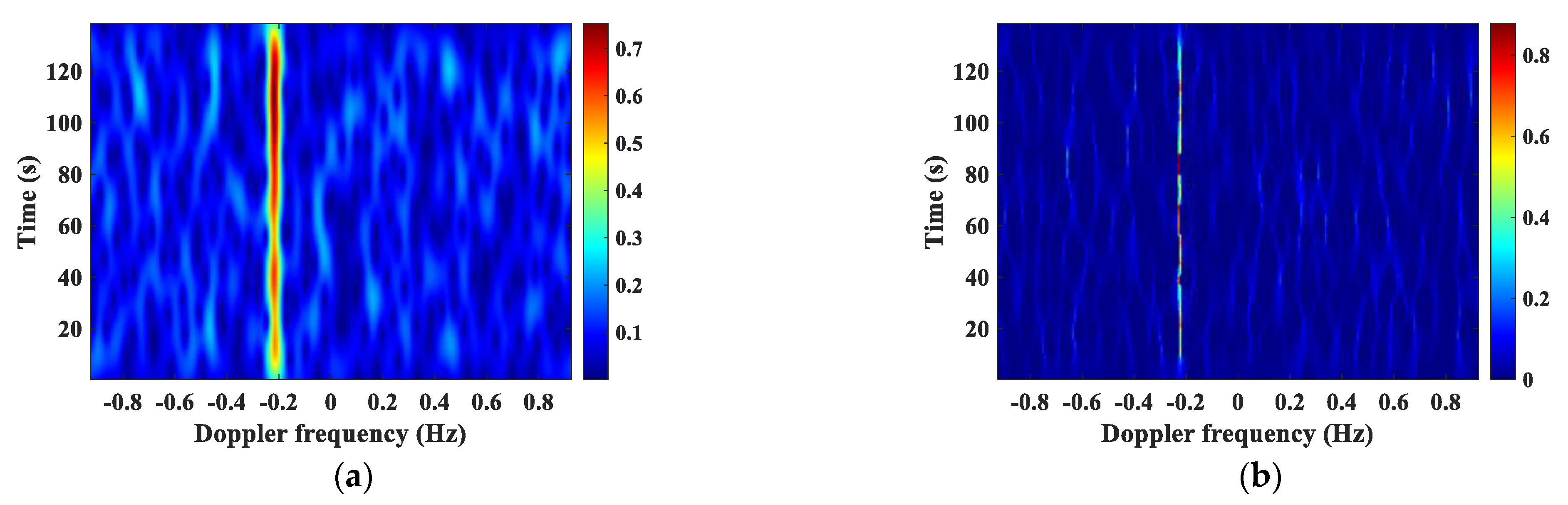
3.1. Denoising
3.2. Non-CFAR Detection
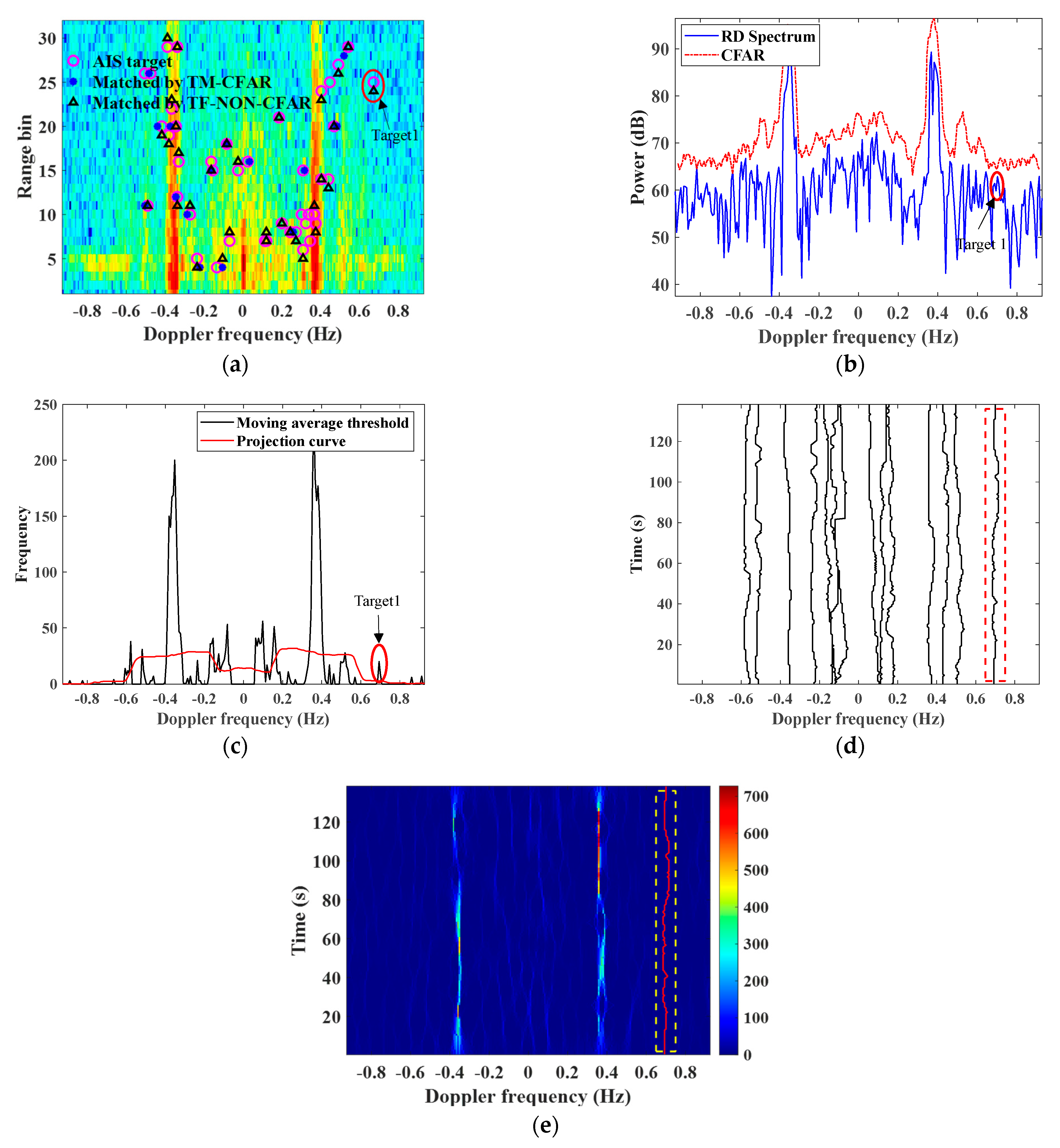
3.2.1. Ship Target Detection in Noise Regions
3.2.2. Statistical Analysis of Target Detection in Noise Regions
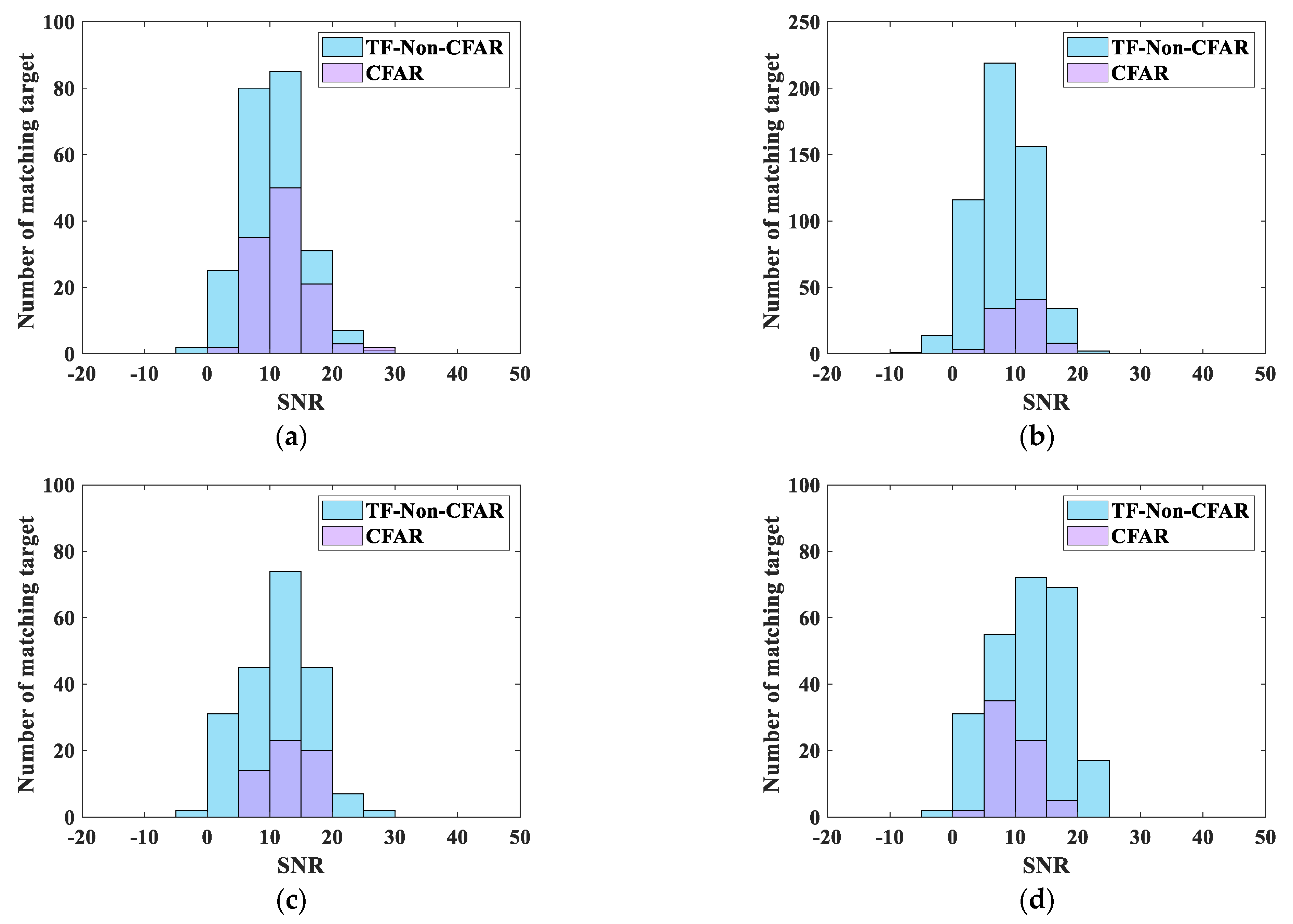
3.2.3. SNR Distribution of Matching Target in Noise Regions
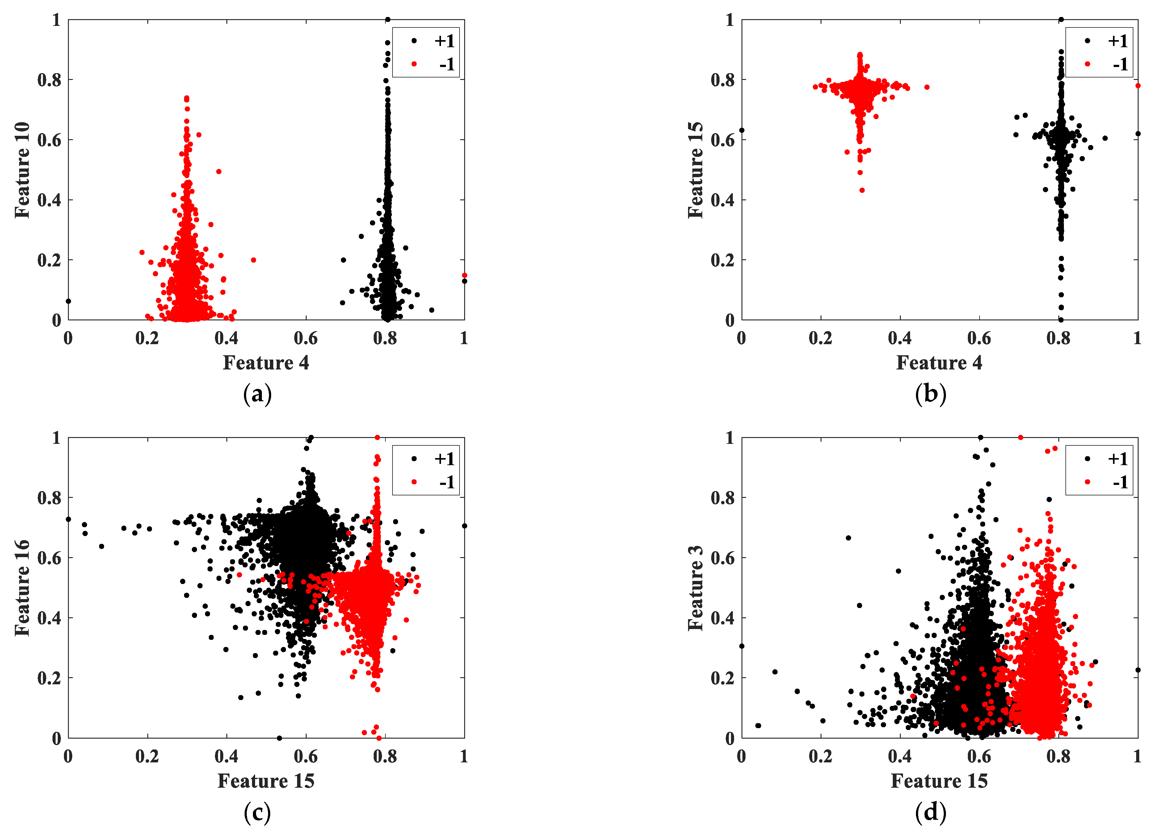
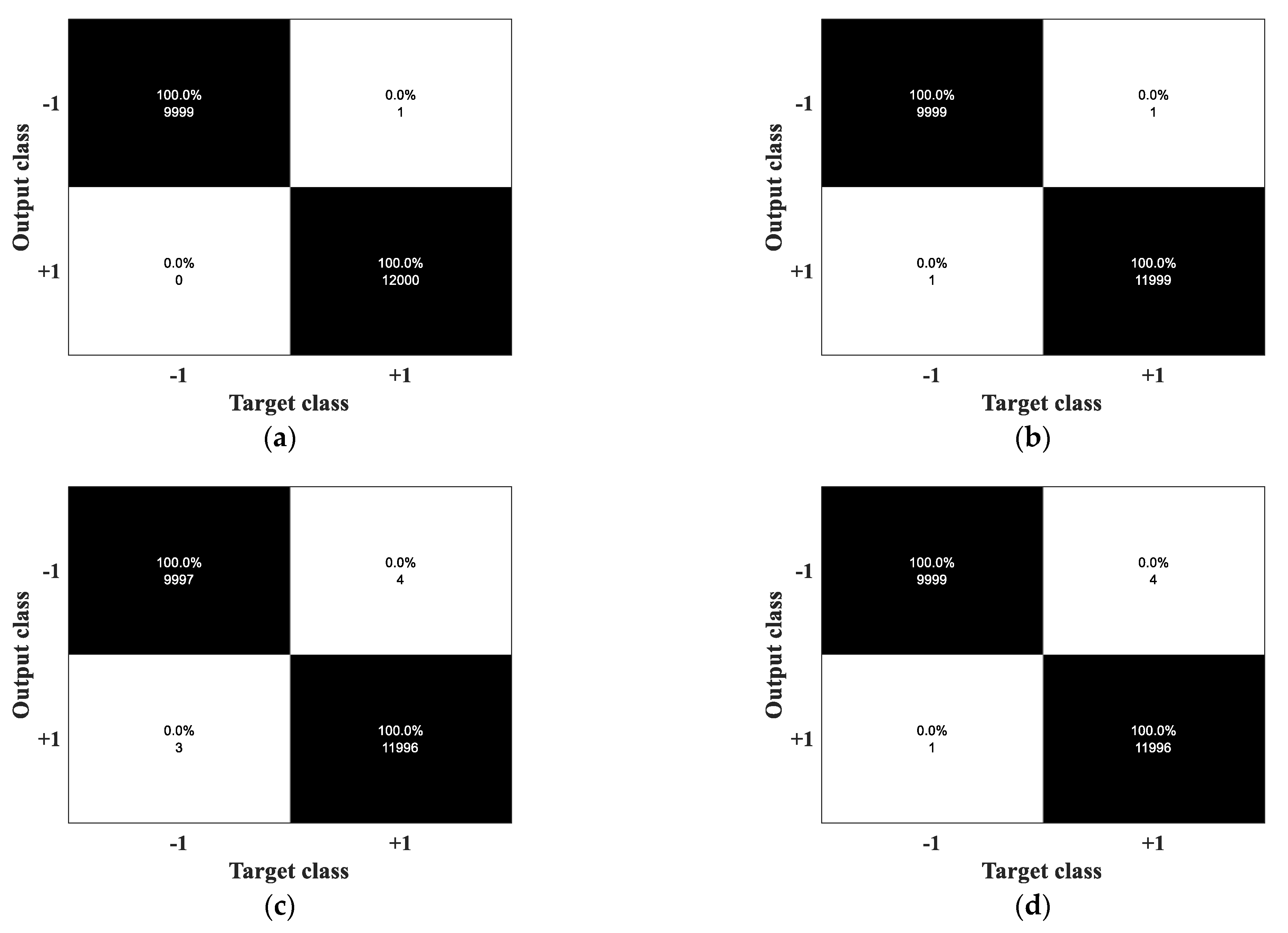
3.3. Statistical Analysis of Matching Targets
4. Discussion
5. Conclusions
Author Contributions
Funding
Data Availability Statement
Acknowledgments
Conflicts of Interest
Abbreviations
| HFSWR | High-Frequency Surface Wave Radar |
| SNR | Signal to Noise |
| TF | Time–Frequency |
| CFAR | Constant False Alarm Rate |
| RCS | Radar Cross Section |
| CA | Cell Averaging |
| GO | Greatest of |
| SO | Smallest of |
| OS | Ordered Statistics |
| CMLD | Censored Mean Level Detector |
| TM | Trimmed-Mean |
| S-CFAR | Switching-CFAR |
| E-CFAR | Ensemble-CFAR |
| GM | Geometric Mean |
| VI | Variability Index |
| TI | Test Inclusive |
| FOD | First-Order Difference |
| SOD | Second-Order Difference |
| BVI | Bayesian Variability Index |
| HF | High Frequency |
| RD | Range Doppler |
| STFT | Short Time Fourier transform |
| DWT | Discrete Wavelet Transform |
| PCA | Principal Component Analysis |
| TFA | Time–Frequency Analysis |
| 1D | One-Dimensional |
| 2D | Two-Dimensional |
| SET | Synchronous Extraction Transform |
| TF-BI-CFAR | Time–Frequency Binary Integration-CFAR |
| SST | Synchrosqueezed Transform |
| CIT | Coherent Integration Time |
| AIS | Automatic Identification System |
| TF-Non-CFAR | Time–Frequency Non-CFAR |
| OSMAR | Ocean State Measuring and Analyzing Radar |
| SD | S stands for Small, Smart, and Super, and D stands for Digital |
| KNN | K-Nearest Neighbor |
| DT | Decision Tree |
| SVM | Support Vector Machine |
| NN | Neural Network |
| Pd | Detection Probability |
| Pfa | False Alarm Probability |
References
- Golubović, D.; Erić, M.; Vukmirović, N.; Orlić, V. High-Resolution Sea Surface Target Detection Using Bi-Frequency High-Frequency Surface Wave Radar. Remote Sens. 2024, 16, 3476. [Google Scholar] [CrossRef]
- Lisowski, J.; Szklarski, A. Quality Analysis of Small Maritime Target Detection by Means of Passive Radar Reflectors in Different Sea States. Remote Sens. 2022, 14, 6342. [Google Scholar] [CrossRef]
- Liu, G.; Tian, Y.; Yang, J.; Ma, S.; Wen, B. High-Speed Target Tracking Method for Compact HF Radar. IEEE J. Sel. Top. Appl. Earth Obs. Remote Sens. 2024, 17, 13276. [Google Scholar] [CrossRef]
- Yen, S.; Boskovic, L.; Filipovic, D. An HF-Band Linear Retrodirective Array with Scale Model RCS Measurements. IEEE Trans. Antennas Propag. 2024, 72, 5822. [Google Scholar] [CrossRef]
- Zhang, J.; Zhu, Q.; Huang, D.; Zhou, H.; Tian, Y. Biologically Inspired DOA Estimation Method for Small-Aperture Direction Finding HF Radar. IEEE Geosci. Remote Sens. Lett. 2024, 21, 1. [Google Scholar] [CrossRef]
- Li, S.; Wu, X.; Chen, S.; Deng, W.; Zhang, X. Multi-Target Pairing Method Based on PM-ESPRIT-like DOA Estimation for T/R-R HFSWR. Remote Sens. 2024, 16, 3128. [Google Scholar] [CrossRef]
- Finn, H.; Johnson, R. Adaptive detection mode with threshold control as a function of spatially sampled clutter level estimates. RCA Rev. 1968, 29, 414–464. [Google Scholar]
- Trunk, G. Range Resolution of Targets Using Automatic Detectors. IEEE Trans. Aerosp. Electron. Syst. 1978, 14, 750–755. [Google Scholar] [CrossRef]
- Hansen, V.; Sawyers, J. Detectability Loss Due to Greatest of Selection in a Cell-Averaging CFAR. IEEE Trans. Aerosp. Electron. Syst. 1980, 16, 115–118. [Google Scholar] [CrossRef]
- Rohling, H. Radar CFAR thresholding in clutter and multiple target situations. IEEE Trans. Aerosp. Electron. Syst. 1983, 19, 608–621. [Google Scholar] [CrossRef]
- Rickard, J.; Dillard, G. Adaptive detection algorithms for multiple target situations. IEEE Trans. Aerosp. Electron. Syst. 1977, 13, 338–343. [Google Scholar] [CrossRef]
- Blake, S. OS-CFAR theory for multiple targets and nonuniform clutter. IEEE Trans. Aerosp. Electron. Syst. 1988, 24, 785–790. [Google Scholar] [CrossRef]
- Tabet, L.; Soltani, F. A generalized switching CFAR processor based on test cell statistics. Signal Image Video Process. 2009, 3, 256. [Google Scholar] [CrossRef]
- Zhang, R.; Sheng, W.; Ma, X. Improved switching CFAR detector for non-homogeneous environments. Signal Process. 2013, 93, 35. [Google Scholar] [CrossRef]
- Srinivasan, R. Robust radar detection using ensemble CFAR processing. IEEE Proc. Radar Sonar Navigat. 2000, 147, 291–297. [Google Scholar] [CrossRef]
- Smith, M.; Varshney, P. Intelligent CFAR processor based on data variability. IEEE Trans. Aerosp. Electron. Syst. 2000, 36, 837–847. [Google Scholar] [CrossRef]
- Kim, J.; Bell, M. A Computationally Efficient CFAR Algorithm Based on a Goodness-of-Fit Test for Piecewise Homogeneous Environments. IEEE Trans. Aerosp. Electron. Syst. 2013, 49, 1519–1535. [Google Scholar] [CrossRef]
- Jiang, W.; Huang, Y.; Yang, J. Automatic Censoring CFAR Detector Based on Ordered Data Difference for Low-Flying Helicopter Safety. Sensors 2016, 16, 1055. [Google Scholar] [CrossRef] [PubMed]
- Ali, A.; Hamza, B.; Ahcene, B.; Tarek, M.; Faouzi, S. Generalized Closed-Form Expressions for CFAR Detection in Heterogeneous Environment. IEEE Geosci. Remote Sens. Lett. 2018, 15, 1011–1015. [Google Scholar]
- Weinberg, G. Interference control in sliding window detection processes using a Bayesian approach. Digit. Signal Process. 2020, 99, 102658. [Google Scholar] [CrossRef]
- Zhu, X.; Tu, L.; Zhou, S.; Zhang, Z. Robust Variability Index CFAR Detector Based on Bayesian Interference Control. IEEE Trans. Geosci. Remote Sens. 2022, 60, 1–9. [Google Scholar] [CrossRef]
- Zhu, X.; Yang, C.; Zhou, C.; Shi, Z. Bayesian CFAR Detector in Weibull Clutter via Interference Control. In Proceedings of the 2023 IEEE/CIC International Conference on Communications in China, Dalian, China, 10–12 August 2023. [Google Scholar]
- Lei, Z.; Huang, Z. Time-frequency analysis based image processing for maneuvering target detection in HF OTH radar. In Proceedings of the 2009 IET International Radar Conference, Guilin, China, 20–22 April 2009. [Google Scholar]
- Jangal, F.; Saillant, S.; Helier, M. Wavelet Contribution to Remote Sensing of the Sea and Target Detection for a High-Frequency Surface Wave Radar. IEEE Geosci. Remote Sens. Lett. 2008, 5, 552–556. [Google Scholar] [CrossRef]
- Grosdidier, S.; Baussard, A.; Khenchaf, A. Morphological-based source extraction method for HFSW radar ship detection. In Proceedings of the 2010 IEEE International Geoscience and Remote Sensing Symposium, Honolulu, HI, USA, 25–30 July 2010. [Google Scholar]
- Grosdidier, S.; Baussard, A. Ship detection based on morphological component analysis of high-frequency surface wave radar images. IET Radar Sonar Navig. 2012, 6, 813–821. [Google Scholar] [CrossRef]
- Li, Q.; Zhang, W.; Li, M.; Niu, J.; Wu, Q. Automatic Detection of Ship Targets Based on Wavelet Transform for HF Surface Wavelet Radar. IEEE Geosci. Remote Sens. Lett. 2017, 14, 714–718. [Google Scholar] [CrossRef]
- Lu, B.; Wen, B.; Tian, Y.; Wang, R. A Vessel Detection Method Using Compact-Array HF Radar. IEEE Geosci. Remote Sens. Lett. 2017, 14, 2017–2021. [Google Scholar] [CrossRef]
- Cai, J.; Zhou, H.; Huang, W.; Wen, B. Ship Detection and Direction Finding Based on Time-Frequency Analysis for Compact HF Radar. IEEE Geosci. Remote Sens. Lett. 2020, 18, 72–76. [Google Scholar] [CrossRef]
- Yang, Z.; Tang, J.; Zhou, H.; Xu, X.; Tian, Y.; Wen, B. Joint Ship Detection Based on Time-Frequency Domain and CFAR Methods with HF Radar. Remote Sens. 2021, 13, 1548. [Google Scholar] [CrossRef]
- Yang, Z.; Zhou, H.; Tian, Y.; Huang, W.; Shen, W. Improving Ship Detection in Clutter-Edge and Multi-Target Scenarios for High-Frequency Radar. Remote Sens. 2021, 13, 4305. [Google Scholar] [CrossRef]
- Qu, Y.; Mao, X.; Hou, Y.; Li, X. An RD-Domain Virtual Aperture Extension Method for Shipborne HFSWR. Remote Sens. 2024, 16, 3929. [Google Scholar] [CrossRef]
- Qu, Y.; Mao, X.; Tang, Z.; Wang, Y. A Virtual Aperture Extension Method for Shipborne HFSWR Based on RD-Domain Spatiotemporal Data Block Extrapolation. IEEE Trans. Radar Syst. 2025, 3, 818–831. [Google Scholar] [CrossRef]
- Daubechies, I.; Lu, J.; Wu, H. Synchrosqueezed wavelet transforms: An empirical mode decomposition-like tool. Appl. Comput. Harmon Anal. 2011, 30, 243–261. [Google Scholar] [CrossRef]
- Jia, F.; Lei, Y.; Shan, H.; Lin, J. Early Fault Diagnosis of Bearings Using an Improved Spectral Kurtosis by Maximum Correlated Kurtosis Deconvolution. Sensors 2015, 15, 29363–29377. [Google Scholar] [CrossRef] [PubMed]
- Jones, D.; Parks, T. A high resolution data-adaptive time-frequency representation. IEEE Trans. Signal Process. 1990, 38, 2127–2135. [Google Scholar] [CrossRef]
- Peng, L.; Zhang, T.; Liu, Y.; Li, M.; Peng, Z. Infrared Dim Target Detection Using Shearlet’s Kurtosis Maximization under Non-Uniform Background. Symmetry 2019, 11, 723. [Google Scholar] [CrossRef]
- Baraniuk, R.; Flandrin, P.; Janssen, A.; Michel, O. Measuring time-frequency information content using the Renyi entropies. IEEE Trans. Inf. Theory. 2001, 47, 1391–1409. [Google Scholar] [CrossRef]
- Golshani, L.; Pasha, E.; Yari, G. Some properties of Renyi entropy and Renyi entropy rate. Inf. Sci. 2009, 179, 2426–2433. [Google Scholar] [CrossRef]
- Zack, G.; Rogers, W.; Latt, S. Automatic-measurement of Sister Chromatid Exchange Frequency. J. Histochem. Cytochem. 1977, 25, 741–753. [Google Scholar] [CrossRef] [PubMed]
- Tian, Y.; Wen, B.; Tan, J.; Li, K.; Yan, Z.; Yang, J. A new fully-digital HF radar system for oceanographical remote sensing. IEICE Electron. Express. 2013, 14, 1–6. [Google Scholar] [CrossRef]
- Mu, Y.; Liu, X.; Wang, L.; Asghar, A. A parallel tree node splitting criterion for fuzzy decision trees. Concurr. Comp. Pract. Exp. 2019, 31, 5268. [Google Scholar] [CrossRef]
- Li, J.; Guo, C. Method based on the support vector machine and information diffusion for prediction intervals of granary airtightness. J. Intell. Fuzzy Syst. 2023, 44, 6817–6827. [Google Scholar] [CrossRef]
- Halder, R.; Uddin, M.; Uddin, M.; Aryal, S.; Khraisat, A. Enhancing K-nearest neighbor algorithm: A comprehensive review and performance analysis of modifications. J. Big Data 2024, 11, 113. [Google Scholar] [CrossRef]
- Wan, C.; Si, W.; Deng, Z. Research on modulation recognition method of multi-componentradar signals based on deep convolution neural network. IET Radar Sonar Nav. 2023, 17, 1313–1326. [Google Scholar] [CrossRef]
- Lu, L.; Bu, C.; Su, Z.; Guan, B.; Yu, Q.; Pan, W.; Zhang, Q. Generative deep-learning-embedded asynchronous structured light for three-dimensional imaging. Adv. Photonics 2024, 6, 46004. [Google Scholar] [CrossRef]
- Yu, Y.; Li, W.; Bai, L.; Duan, J.; Zhang, X. UTDM: A universal transformer-based diffusion model for multi-weather-degraded images restoration. Visual Comput. 2024, 6, 4269–4285. [Google Scholar] [CrossRef]


| Parameter | Value |
|---|---|
| Carrier frequency (MHz) | 13.15 |
| Sweep band (kHz) | 60 |
| Range resolution (km) | 2.5 |
| Velocity resolution (m/s) | 0.0825 |
| Receive antenna | Cross-Loop/Monopole |
| Sweep cycle (s) | 0.54 |
| Coherent integration time (CIT) (s) | 138.24 |
| Method | Date | Detected Number | Matched Number | Matching Rate (%) |
|---|---|---|---|---|
| Without denoising | 22 September | 145,217 | 15,893 | 10.94 |
| 6 October | 156,171 | 13,712 | 8.78 | |
| 15 November | 156,332 | 16,454 | 10.52 | |
| Denoising | 22 September | 139,362 | 15,814 | 11.34 |
| 6 October | 139,520 | 13,675 | 9.80 | |
| 15 November | 139,556 | 16,405 | 11.75 |
| Method | Detected Number of Noise Region | Matched Number of Noise Region | Matching Rate (%) |
|---|---|---|---|
| CA-CFAR | 9856 | 123 | 1.24 |
| OS-CFAR | 9023 | 102 | 1.13 |
| TM-CFAR | 9328 | 113 | 1.21 |
| CMLD-CFAR | 9265 | 123 | 1.32 |
| VI-CFAR | 9653 | 124 | 1.28 |
| FOD-CFAR | 8741 | 79 | 0.90 |
| SOD-CFAR | 10,344 | 105 | 1.01 |
| BVI-CFAR | 9303 | 114 | 1.22 |
| TF-BI-CFAR | 4574 | 335 | 7.32 |
| TF-Non-CFAR | 743 | 269 | 36.20 |
| SNR | Date | CFAR | TF-Non-CFAR |
|---|---|---|---|
| <10 dB | 22 September | 37 | 107 |
| 25 September | 37 | 350 | |
| 6 October | 14 | 78 | |
| 15 November | 37 | 88 | |
| ≥10 dB | 22 September | 76 | 124 |
| 25 September | 49 | 192 | |
| 6 October | 43 | 128 | |
| 15 November | 28 | 158 |
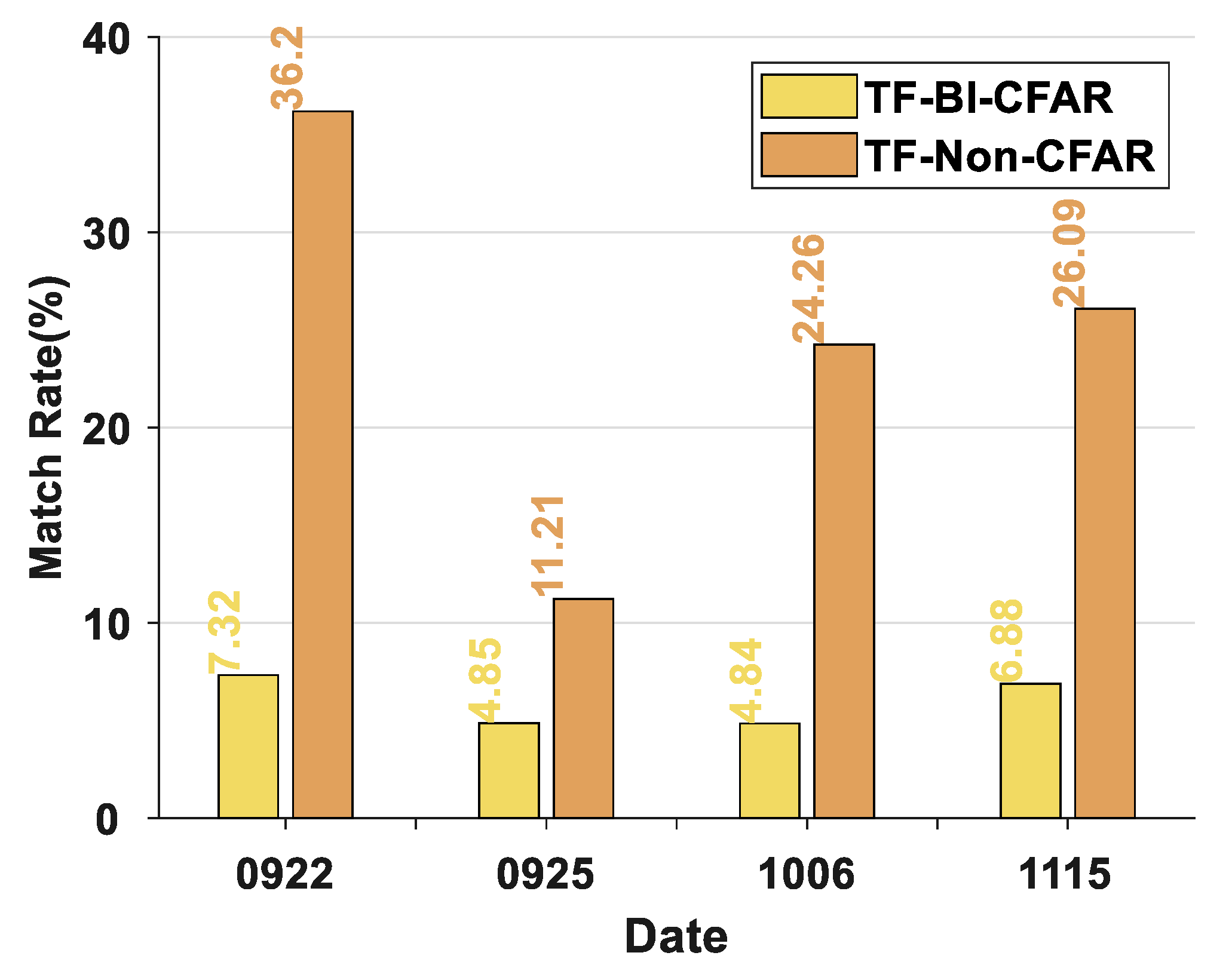
| Method | Date | Detected Number of Noise Region | Matched Number of Noise Region | Matching Rate (%) |
|---|---|---|---|---|
| TF-BI-CFAR | 22 September | 4574 | 335 | 7.32 |
| 25 September | 6036 | 293 | 4.85 | |
| 6 October | 3946 | 191 | 4.84 | |
| 15 November | 3661 | 252 | 6.88 | |
| TF-Non-CFAR | 22 September | 743 | 269 | 36.20 |
| 25 September | 2479 | 278 | 11.21 | |
| 6 October | 647 | 157 | 24.26 | |
| 15 November | 778 | 203 | 26.09 |
Disclaimer/Publisher’s Note: The statements, opinions and data contained in all publications are solely those of the individual author(s) and contributor(s) and not of MDPI and/or the editor(s). MDPI and/or the editor(s) disclaim responsibility for any injury to people or property resulting from any ideas, methods, instructions or products referred to in the content. |
© 2025 by the authors. Licensee MDPI, Basel, Switzerland. This article is an open access article distributed under the terms and conditions of the Creative Commons Attribution (CC BY) license (https://creativecommons.org/licenses/by/4.0/).
Share and Cite
Yang, Z.; Zhou, H.; Tian, Y.; Liu, G.; Zhang, B.; Qin, Y.; Li, P.; Huang, W. Cascaded Detection Method for Ship Targets Using High-Frequency Surface Wave Radar in the Time–Frequency Domain. Remote Sens. 2025, 17, 2580. https://doi.org/10.3390/rs17152580
Yang Z, Zhou H, Tian Y, Liu G, Zhang B, Qin Y, Li P, Huang W. Cascaded Detection Method for Ship Targets Using High-Frequency Surface Wave Radar in the Time–Frequency Domain. Remote Sensing. 2025; 17(15):2580. https://doi.org/10.3390/rs17152580
Chicago/Turabian StyleYang, Zhiqing, Hao Zhou, Yingwei Tian, Gan Liu, Bing Zhang, Yao Qin, Peng Li, and Weimin Huang. 2025. "Cascaded Detection Method for Ship Targets Using High-Frequency Surface Wave Radar in the Time–Frequency Domain" Remote Sensing 17, no. 15: 2580. https://doi.org/10.3390/rs17152580
APA StyleYang, Z., Zhou, H., Tian, Y., Liu, G., Zhang, B., Qin, Y., Li, P., & Huang, W. (2025). Cascaded Detection Method for Ship Targets Using High-Frequency Surface Wave Radar in the Time–Frequency Domain. Remote Sensing, 17(15), 2580. https://doi.org/10.3390/rs17152580