Article

How Reliable Are the Spectral Vegetation Indices for the Assessment of Tree Condition and Mortality in European Temporal Forests?

1
Institute of Environmental Protection–National Research Institute, 32 Słowicza Street, 02-170 Warsaw, Poland
2
Department of Forest Resources Management, Faculty of Forestry, University of Agriculture in Krakow, 31-120 Krakow, Poland
*
Author to whom correspondence should be addressed.
Remote Sens. 2025, 17(15), 2549; https://doi.org/10.3390/rs17152549
Submission received: 10 June 2025 / Revised: 7 July 2025 / Accepted: 18 July 2025 / Published: 23 July 2025

Abstract

The continuous monitoring of forest vegetation conditions is of the utmost importance. The commonly used tools for assessing vegetation conditions are the normalized difference vegetation index (NDVI) and its successor—the enhanced vegetation index (EVI). In this study, the NDVI and EVI were coupled with the data on the number of dead trees removed during sanitation felling in an area of 13,780 km2 during the period 2015–2022. In order to determine which satellite-borne index best represents the actual condition of vegetation in forests of the European temperate zone, the classes of the trend in changes in the NDVI and EVI were compared with the respective trends in the volume of dead trees, following the assumption that a positive trend in the spectral index values should be reflected by a negative trend in the volume of dead trees, and vice versa. The analyses were carried out for pixels within the all-species mask in the study area and for pixels representing individual tree species. NDVI is a good predictor of forest vegetation in the European temperate zone and is substantially better than EVI. Spatially, NDVI yields more pixels showing a negative slope for the trend in changes in the spectral index values, while EVI seems to overestimate the number of positive slopes. A larger number of negative slopes in the trend in changes in NDVI seems to agree with the increasing volume of dead trees in the analysed period. Comparing the detected trend class masks for spectral indices and the multi-annual course of dead trees, in 12 out of 16 cases, the slopes of the trend in changes in NDVI agree with the slopes of the trend in the volume of dead trees, while for EVI, this number is reduced to 9. In addition, NDVI reflects the condition of coniferous tree species, Scots pine and Norway spruce, substantially better.

1. Introduction

One of the essential components of the biosphere is forest vegetation. With almost 31% of land coverage [1] and a contribution of up to 3/4 of the gross primary production of the Earth’s biosphere [2], forest is the world’s predominant terrestrial ecosystem. A forest presence in a particular place can help protect water, soil, ecosystems, and infrastructures [3]. Forests significantly reduce soil erosion, play an important role in carbon sequestration and evaporative cooling processes across the globe and hence mitigate climate change. The continuous monitoring of forest vegetation conditions is of paramount importance for assessing forest growth and yield and detecting problems related to water shortages or tree diseases that affect forest ecosystem services.
Remote sensing has emerged as the most significant tool used worldwide to quantify the vegetation dynamics and its relationship with variations in meteorological elements, induced by climate change. Using spectral characteristics of the plant, satellite remote sensing enables the evaluation of vegetation vigour. The most commonly used tool for assessing vegetation—with a long 50-year history in the research of vegetation vigour—is the normalized difference vegetation index (NDVI) [4,5,6,7]. The NDVI formula uses the near-infrared-to-red reflectance ratio and is designed to standardise vegetation index values to between −1 and +1 [8]. It is considered a reliable ecological indicator, given its derivation from thoroughly calibrated satellite-borne sensors [6]. NDVI is chlorophyll-sensitive and adequately reflects the changes in leaf colouration, e.g., in the course of drought-induced premature leaf senescence [5]. However, its major limitation is the saturation effect, i.e., insensitivity to changes after a certain level of biomass is reached [9]. For deciduous forests, this level has been set at 100 Mg·ha−1 [10]. This is very important in forest condition monitoring and assessment, considering that NDVI is calculated from the signal coming from the entire thickness of the multi-storey forest, including the understorey, undergrowth, and the ground surface lying below the canopy layer [6].
A successive indicator to NDVI, the enhanced vegetation index (EVI), was created to address the issue of reflected light distortions caused by atmospheric particles and the ground cover below the vegetation, hence improving upon NDVI limitations [11]. In addition to using red and near-infrared radiation, the EVI formula also uses blue radiation to stabilise the index values against changes in the levels of aerosol concentration [8]. Contrary to NDVI, EVI is more sensitive to structural variations of the canopy [11]; hence, it is supposed to better reflect early leaf shedding [5]. In addition, EVI does not saturate as quickly as NDVI [9].
Many studies so far have solely used NDVI [12,13,14,15,16,17,18] or EVI [19,20,21,22] to assess the vegetation condition. Some studies suggest that results obtained with NDVI are generally confirmed by the analyses using EVI [5], while others show some differences between both indicators’ results [23,24,25]. According to [26], EVI was more suitable than NDVI when assessing phenology in evergreen species of the northern boreal forest in Canada (2016–2019). In addition, [27], who researched silver fir stands in the Spanish Pyrenees (1984–2023), indicated that EVI better reflected the early responses of forest stands to climatic stress, and hence it is preferable over the NDVI. However, they suggest that the information provided by NDVI and EVI is somehow complementary, rather than exclusive. Contrary to that, on the basis of Moderate Resolution Imaging Spectroradiometers (MODIS) data from 2008, ref. [24] found that NDVI had higher correlations with in situ data on vegetation cover (grassland, shrub, and forest) than EVI; so, NDVI was better for predicting natural vegetation coverage in the humid continental climate of the temperate zone. MODIS NDVI also had a good relationship with oak productivity in the Mediterranean climate of Portugal (1984–2017) [28].
Such contrasting conclusions raise the need to further investigate the performance of NDVI and EVI, especially in relation to a complex multi-storey forest ecosystem. In order to correctly assess which of the satellite-borne indicators better reflects the ‘ground truth’, i.e., the actual condition of forest vegetation, in situ data are needed. These data require field research and are often difficult or expensive to produce. For this reason, such comparative studies are still very limited in the European temperate zone [29].
Natural disturbances, such as fire, wind, snow, drought, and insects, significantly influence forest condition and—consequently—influence the forest mortality dynamics [30]. The condition of the forest vegetation might be thus approximated using data on the volume of dead trees removed from the individual forest stands during sanitation felling (it does not include the volume of wood obtained as part of the planned tree felling). In the managed forest stands, the volume of trees removed through sanitation felling—that is, the selective removal of dead, dying, or pest-infested trees—may serve as a useful proxy for the overall stand condition. Because such operations are typically conducted in response to mortality events—abiotic (e.g., windthrow or drought) or biotic (e.g., insect outbreaks)—the cumulative volume removed over a defined period can closely approximate actual mortality rates, which are widely recognised as integrative indicators of forest health [31,32]. Hence, the wood volume removed during sanitation felling is a crucial indicator of the forest disturbance [33]. Such data can be used as a reference for modelling forest stand mortality [34,35].
In this study, we couple the MODIS-based NDVI and EVI with the data on the number of trees removed during sanitation felling. We hypothesise that multi-annual trends in changes in the spectral indicators should be reflected in the respective trend in the volume of dead trees removed during sanitation felling. With a unique and very extensive dataset of volume of dead trees, gathered as a result of sanitation felling in the area of approx. 13,780 km2 (in three regional directorates of state forest in Poland) over eight years (2015–2022), we aim to determine which of the spectral indices (NDVI or EVI) reflects better the actual condition of vegetation in the forests of the European temperate zone. Thus, the main objectives of this research are (1) to identify the trend in changes in NDVI and EVI and temporal variations in the volume of dead trees during the period 2015–2022 and (2) to couple the detected trends in NDVI and EVI with the volume of dead trees removed during sanitation felling, in order to assess which satellite-borne index best represents the actual forest condition. To make the research results more comprehensive, the analyses were carried out for all forest pixels in the study area and for pixels representing individual tree species.

2. Materials and Methods
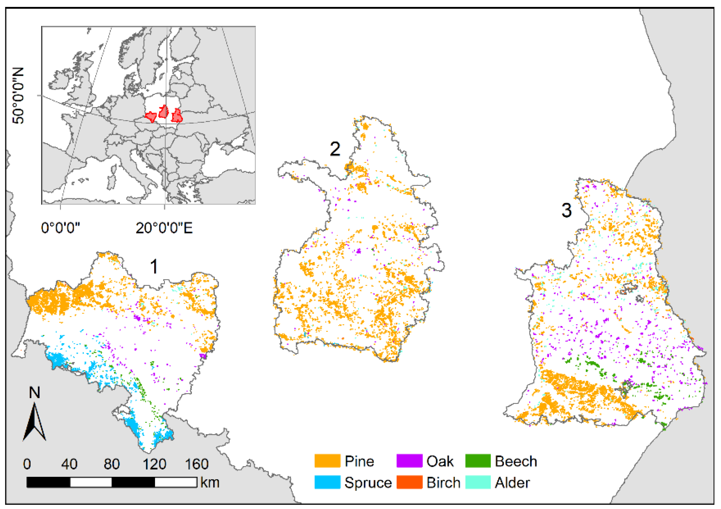
2.1. Study Area

The study area consists of the three regional directorates of state forest in Poland: Wroclaw, Lodz, and Lublin (marked with ‘1’, ‘2’, and ‘3’ in Figure 1, respectively). The forests there are mostly managed, because the national parks and areas of strict protection are excluded from directorates’ jurisdiction. The dominant landscape in the study area is composed of lowlands (mostly Lodz and northern parts of Wroclaw and Lublin regions), and uplands (parts of Wroclaw and Lublin regions), with mountains in the south of Wroclaw state forest directorate (the Sudeten mountains). The study area adequately represents the conditions of a European warm temperate climate, with a mean annual temperature of 8.4 °C, and mean annual precipitation from 500 to 700 mm. Severe mountain conditions occur only in the mountains in the south of the Wroclaw state forest directorate (mean annual temperature of 1.5 °C and mean annual precipitation of 1200 mm) (1991–2020) [36].
The most widespread and dominant species in the study area is Scots pine (Pinus sylvestris L.; hereafter pine) [37], which is quite well adapted to living in warm and cold temperate zones and in nutrient-poor soils. It grows mostly in the lowlands and often in a form of a planted monoculture, covering 62% of the forest area of the three state forest directorates. Contrary to pine, broadleaved species, e.g., oak species (Quercus petraea (Matt.) Liebl., Quercus robur L.; hereafter oak), have more site requirements. Oaks clusters are present in the lowlands and uplands of Wroclaw and Lublin regions, occupying up to 14% of the forest area in the Lublin state forest directorate [38]. In the upland and mountain sites, the predominant tree species are European beech (Fagus sylvatica L.; hereafter beech) and Norway spruce (Picea A. Dietr.; hereafter spruce), which occupy mostly Roztocze upland in the Lublin state forest directorate and the foothill, sub-mountain, and mountain regions in the south of the Wroclaw state forest directorate. The share of spruce in Wroclaw directorate exceeds 23% of the forest area [39]. Other species with a noticeable share in the species composition—silver birch (Betula pendula Roth; hereafter birch) and black alder (Alnus glutinosa (L.) Gaertn.; hereafter alder)—grow mostly in the lowlands, but they usually do not form separate clusters, thus they are accompanying species.
A detailed tree species classification, based on a machine learning random forest algorithm, was prepared on the basis of the multi-temporal data from Sentinel-2. It was made following the hierarchical approach [40]. The Sentinel-2 data acquired in the growing season of 2022, in spring (May–June), summer (July–August), and autumn (September–October), combined with the topographical data from the Shuttle Radar Topography Mission Digital Elevation Model (SRTM DEM) were used to classify eight tree species, namely: pine, spruce, larch, fir, oak, birch, beech, and alder. The classification accuracy (F1-score) for pine, spruce, beech, and oak reached 94.5–96.9%, 71.5–93.7%, 86.4–92.9%, and 75.5–84.6% across the three regions respectively. More details about this classification, as well as the description of training and validation data and accuracy assessment, are included in [41].
In order to conduct analyses for the chosen tree species, the respective tree species’ masks in the MODIS grid were produced on the basis of the result of the Sentinel-2 classification. For each MODIS grid cell, the number of Sentinel-2 pixels located inside this MODIS grid cell was calculated. The MODIS grid cell was assigned to a particular species’ mask if at least 90% of the Sentinel-2 pixels was classified as this species. As a result, six separate species masks in the MODIS grid were prepared (two species—fir and larch—did not produce clusters large enough to produce a mask in the MODIS grid), with their spatial distribution presented in Figure 1, and the number of retained MODIS pixels and the covering area presented in Table 1. Because of the low number of pixels in the masks of birch and alder, we excluded them from further analyses. Finally, the masks of pine, spruce, oak, and beech, as well as the mask of all-species (which is a sum of all six masks), were used in this study.

2.2. NDVI and EVI Monthly Values

NDVI and EVI were derived from the Moderate Resolution Imaging Spectroradiometers (MODIS) [42,43]. The products MOD13Q1 (from the Terra satellite) and MYD13Q1 (from the Aqua satellite) are available at the spatial resolution of 250 m and were derived from the NASA EOSDIS Land Processes Distributed Active Archive Center (http://search.earthdata.nasa.gov, accessed on 1 May 2024), for the basic time period 2015–2022 (and separately for the longer time period 2002–2022). We used only the pixels indicated as good or marginal quality (similarly to [5]) and allocated them to appropriate months. Out of all values for a given MODIS grid cell and for a given month, only the maximum one was taken. As in many similar studies, we assumed that low-value observations were either erroneous or had reduced vegetation vigour for the time period under consideration [44]. Having the monthly maximum NDVI (or EVI) values for each MODIS grid cell and for each month during the basic period 2015–2022 (and during the longer period 2002–2022 separately), we produced the standardised NDVI (EVI) values, i.e., z-scores. They were calculated in the same way as in [45], i.e., the monthly mean NDVI (EVI) values were standardised separately for each month (in order to remove the natural annual cycle). Such approach helps to highlight extreme monthly values and thus better determine extreme events, e.g., drought.
In the next step, the slopes for the linear trend in changes in z-scores NDVI (or EVI) were produced for the mask of all-species. The slopes were assessed for statistical significance (α = 0.05) and categorised into five classes: (1) strong negative slopes, which are smaller than the median of all negative statistically significant slopes, (2) moderate negative slopes, which are larger than the median of all negative statistically significant slopes, (3) insignificant slopes, (4) moderate positive slopes, which are smaller than the median of all positive statistically significant slopes, and (5) strong positive slopes, which are larger than the median of all positive statistically significant slopes. The methodology diagram showing the above-described steps is presented in Figure 2.

2.3. Volume of Dead Trees in the Forest Stands

Detailed information on the volume of dead trees removed during sanitation felling as the effect of forest disturbance was derived from the three regional directorates of the state forest in Poland. This did not include the volume of wood obtained as part of planned silvicultural treatments. The volume of dead trees (in m3·year−1) is collected by the forest administration with a resolution to a single forest stand and divided into species. The data include information on causes of mortality, divided into two groups: pest/drought and wind. In this study, only the volume of dead trees related to pest/drought was used. The data are collected yearly; however, before the year 2015, the sanitation felling was reported at the forest district level, which made it useless for this analysis. Hence, the data on the volume of dead trees over eight years, i.e., 2015–2022, were used. A forest stand is a polygon of irregular shape and area ranging from ca. 0.1 ha to ca. 50 ha (typical values in this study area), with a mean area of 5.1 ha. As the borders of the forest stand may change over time, we used separate and up-to-date vector layers of forest stands for each year during the analysed period [46]. In order to perform analyses in this study, we assumed that dead trees were gathered evenly from each part of a forest stand; so, the conversion from m3·year−1 per forest stand into m3·year−1 per hectare was applied. Next, the information was converted from the forest stands to the MODIS grid, based on the weighted average method. The volume of dead trees gathered in the particular MODIS grid cell was calculated according to the following formula (Equation (1)):
V o l u m e   o f   d e a d   t r e e s   M O D y , s = i = 1 n a r e a A i , y , s M O D y , s a r e a M O D y , s × D e a d   t r e e s A i , y , s ,
where MODy,s is the particular MODIS grid cell in the year y and for the species s; Ai,y,s is the i-th forest stand that overlaps MODy,s in the year y and for the species s; n is the number of all forest stands that overlap MODy,s. If dead trees from different species were gathered in the particular MODIS grid cell in the year y, these values were added (Equation (2)):
V o l u m e   o f   d e a d   t r e e s   ( M O D y ) = s = 1 m V o l u m e   o f   d e a d   t r e e s M O D y , s
where m is the number of species.
Having yearly volumes of dead trees for each MODIS grid cell, a mask of dead trees pixels was prepared. A particular MODIS grid cell was assigned into a dead trees mask, if at least in one year the volume of dead trees was larger than zero. Following this selection criterion, 253,399 pixels were retained as the dead trees mask, covering the area of 13,784.9 km2. Only these MODIS grid cells were used for further analysis. The methodology diagram showing the above-described steps is presented in Figure 2.

2.4. Methods

In order to identify the trend in changes in NDVI and EVI and temporal variations in the volume of dead trees, several steps were taken. Firstly, the spatial distribution of the categorised slopes for the trend in changes in z-scores of the NDVI and EVI was presented. Additionally, to illustrate the changes in the vegetation indices’ values in a broader context, the spatially averaged z-scores of the NDVI and EVI in the mask of all-species were analysed during the longer time period 2002–2022. The equations of a linear trend in NDVI and EVI z-scores during the basic period 2015–2022 and the longer period 2002–2022 were generated, and the statistical significance of these trends was assessed (α = 0.05).
From the other side, the spatial distribution of the volume of dead trees was prepared. It was presented in the previously prepared dead trees mask in three individual years of the period 2015–2022. To illustrate the multi-annual course of the dead trees during the analysed period, the volume of dead trees in the individual years was summed up and presented in relation to directorates and species.
In the final step, in order to determine whether NDVI or EVI better reflects the actual forest condition—expressed by the volume of dead trees—the coupling of the detected trends in NDVI and EVI with the course of the volume of dead trees was applied. To this end, five classes of the slopes for the trend in changes in NDVI (or EVI) z-scores were intersected with the species masks, creating five submasks for all-species and five submasks for each of the species (pine, spruce, oak, and beech). All the submasks were intersected with the dead trees mask. The course of yearly volumes of dead trees in all submasks was prepared. To this end, for a given year, the dead trees’ volumes in all MODIS grid cells within the dead trees mask and within a specific submask were spatially averaged. The same pixel does not always appear in both sets (in a specific submask and in a dead trees mask), so the final number of retained pixels might be relatively low (the number of pixels making up the dead trees mask within the given submask is shown in each respective figure). The slopes for the linear trend in changes in the volumes of dead trees were calculated, and their statistical significance was assessed at two levels of significance (α = 0.05 and α = 0.1).

3. Results

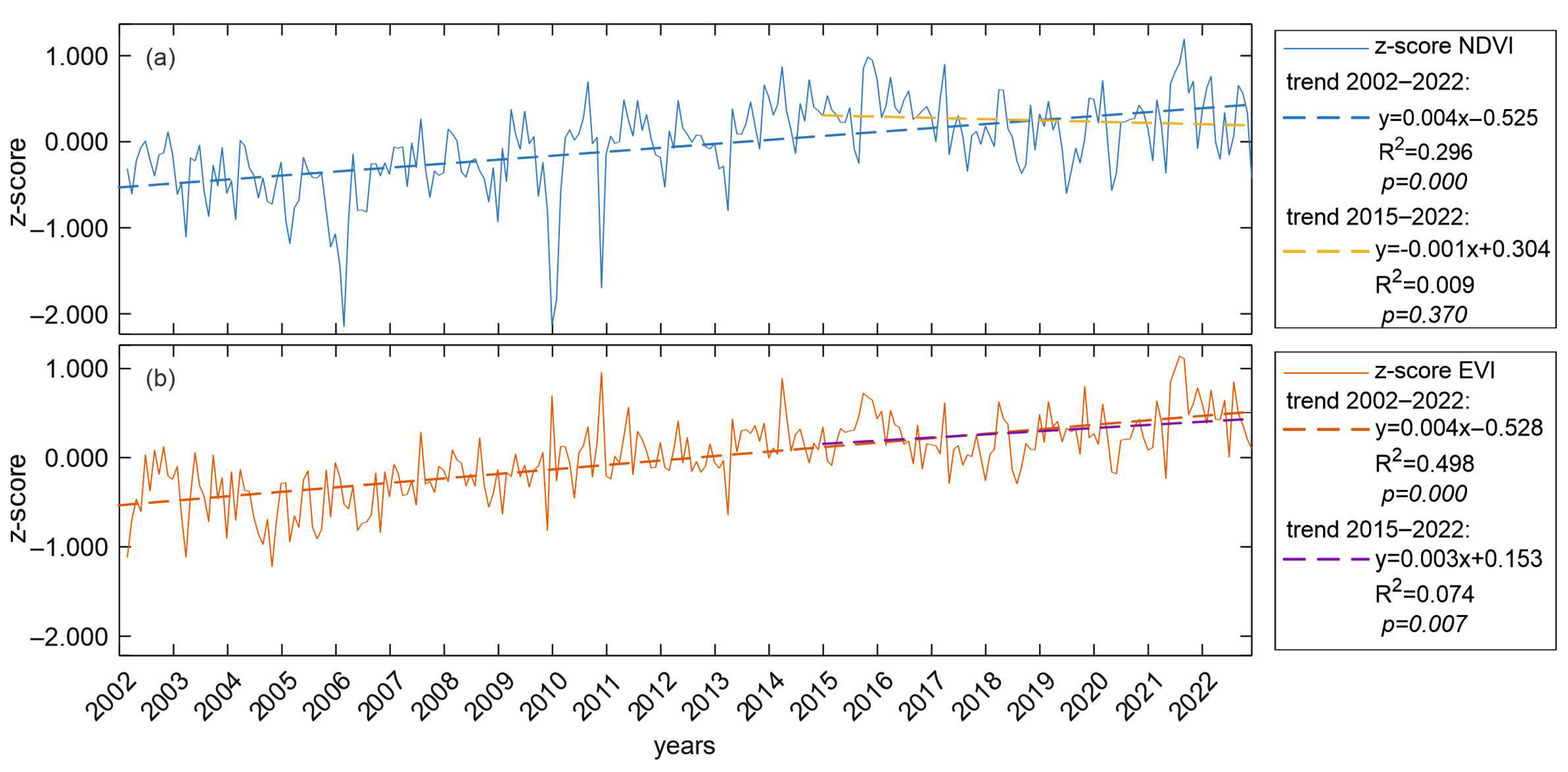
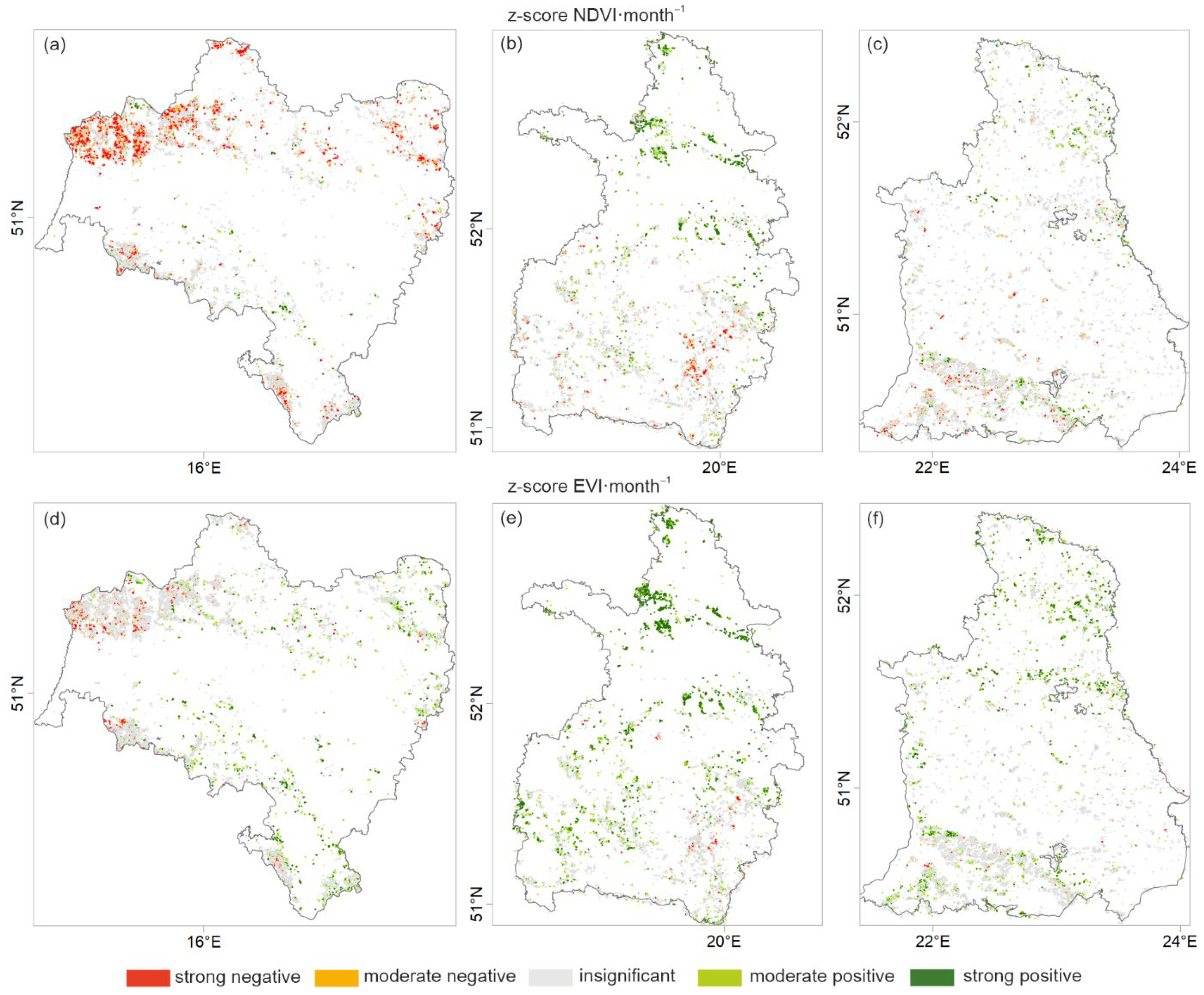
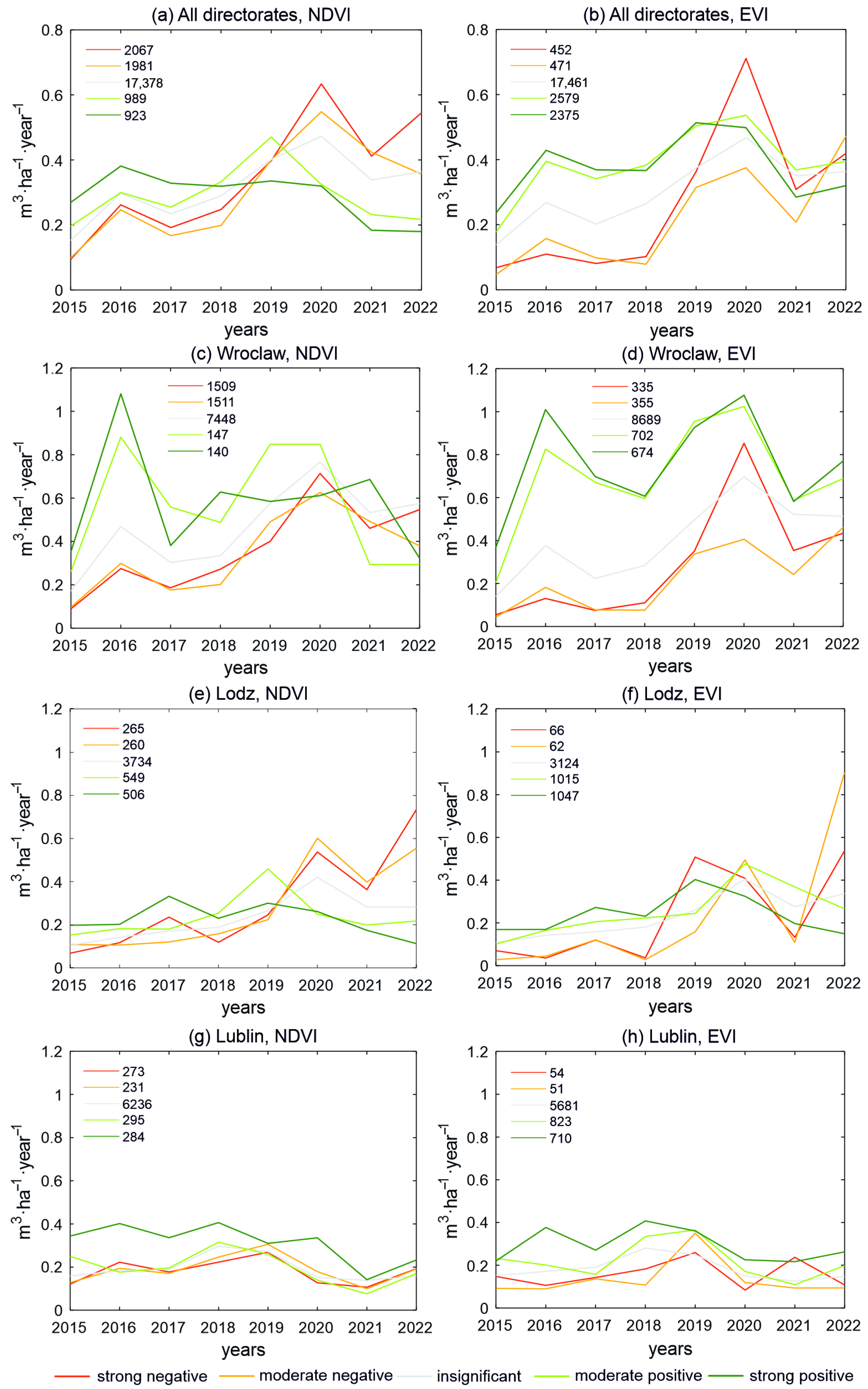
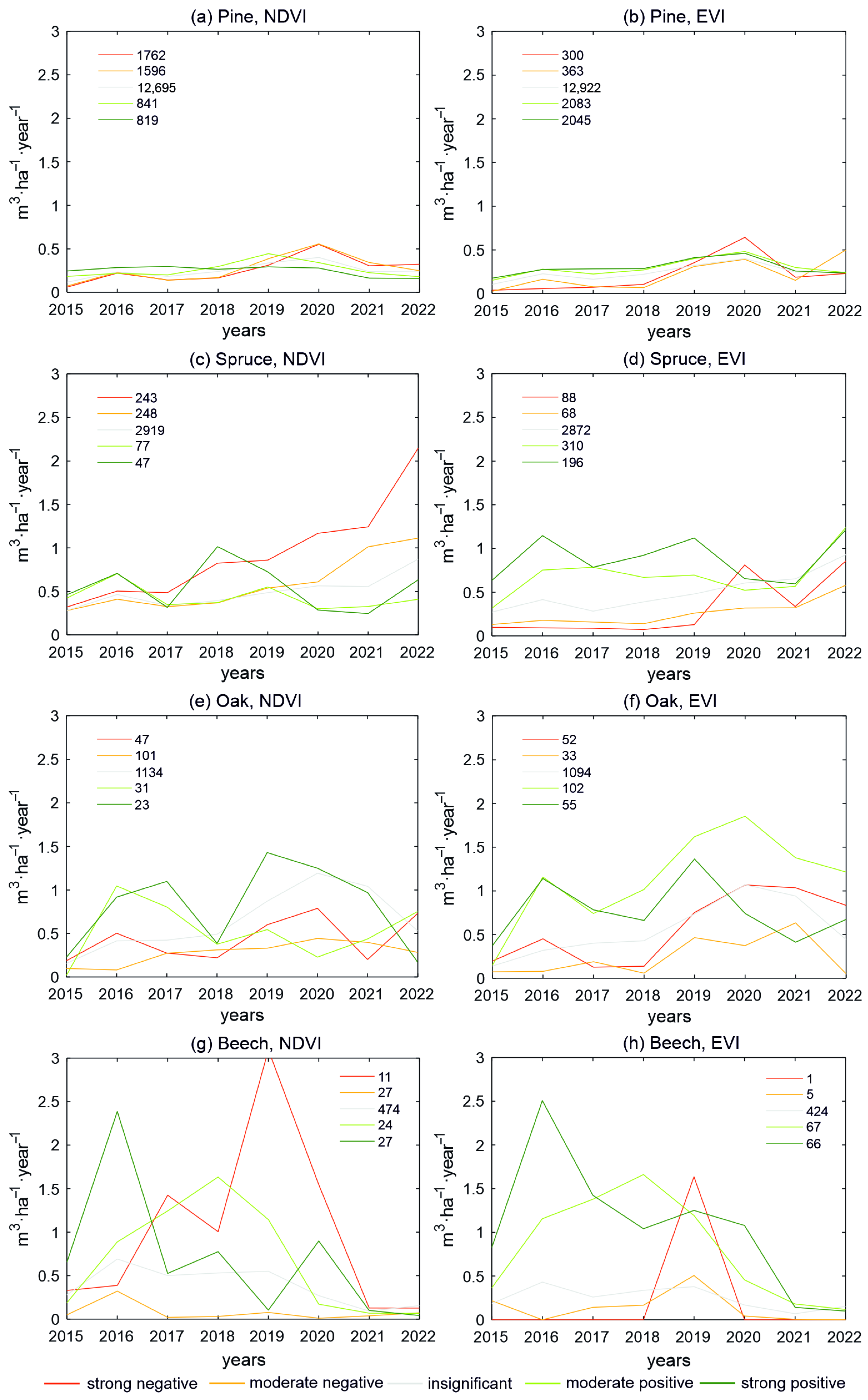
3.1. Trends in Changes in NDVI and EVI Z-Scores

In the last two decades, a general greening of forests was noticed, with a generally increasing trend of 0.004 of the NDVI z-score per month (EVI z-score likewise) (Figure 3). However, the increase in vegetation indices was not stable over time, and during the analysed eight years (i.e., 2015–2022), the trend in changes in NDVI z-scores reversed, while the trend in EVI z-scores was still positive (Figure 3).
In fact, in the period 2015–2022 the spatial distribution of the slopes for the trends in NDVI and EVI z-scores differed (Figure 4). In general, the number of pixels with a statistically significant negative trend was larger for NDVI z-scores than EVI z-scores. At the same time, NDVI z-scores showed fewer pixels with a significant positive trend than EVI z-scores (Table 2). A significant browning can be seen especially in NDVI z-scores in the Wroclaw region (Figure 4a), where the percentage of pixels with the significant negative trend exceeded 28% (Table 2). These are mostly the pixels covered with pine and spruce. However, for the slopes for the trends in EVI z-scores, their spatial distribution in the Wroclaw region was rather different (Figure 4d), with the share of the significant negative trends decreased to 6.90% (Table 2).
Comparing the trend in changes in EVI z-scores to the NDVI z-scores, one can see that many pixels reversed from negative trend values to positive ones, resulting in a generally greening picture. This is mostly the case in the Lodz and Lublin regions, where the share of the significant negative trends dropped from 7.44% and 5.73% (in NDVI z-scores) to 2.49% and 1.17% (in EVI z-scores), respectively (Table 2). At the same time, the percentage of the significant positive trends increased from 20.52% and 9.83% (NDVI z-scores) to 36.75% and 22.82% (EVI z-scores), for Lodz and Lublin, respectively (Table 2).

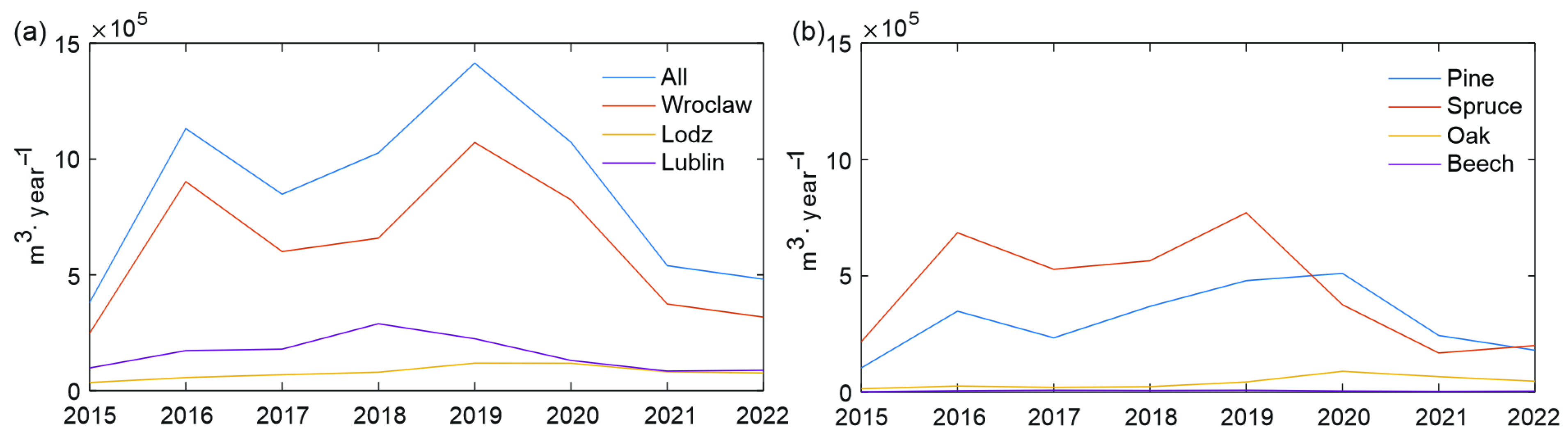
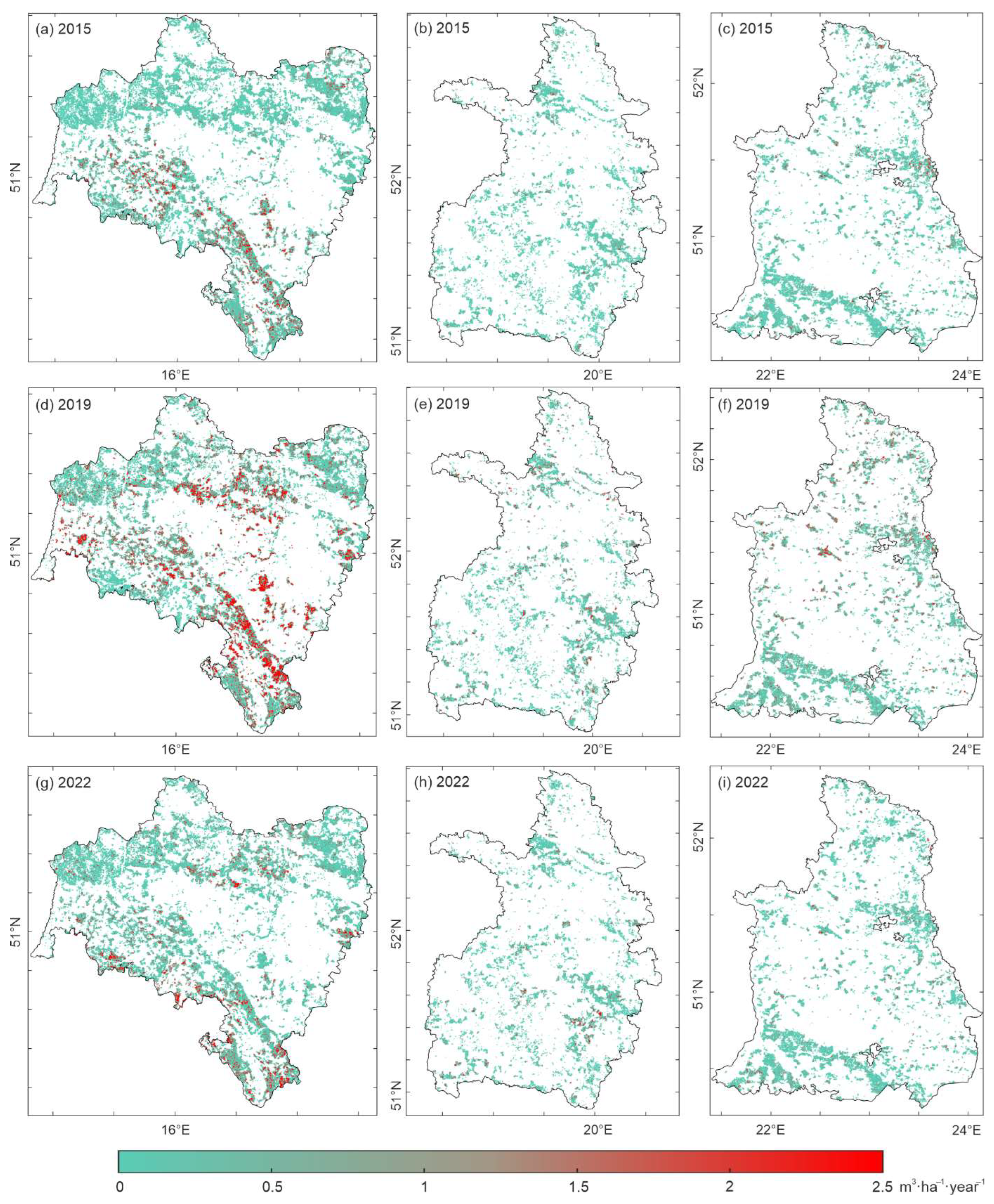
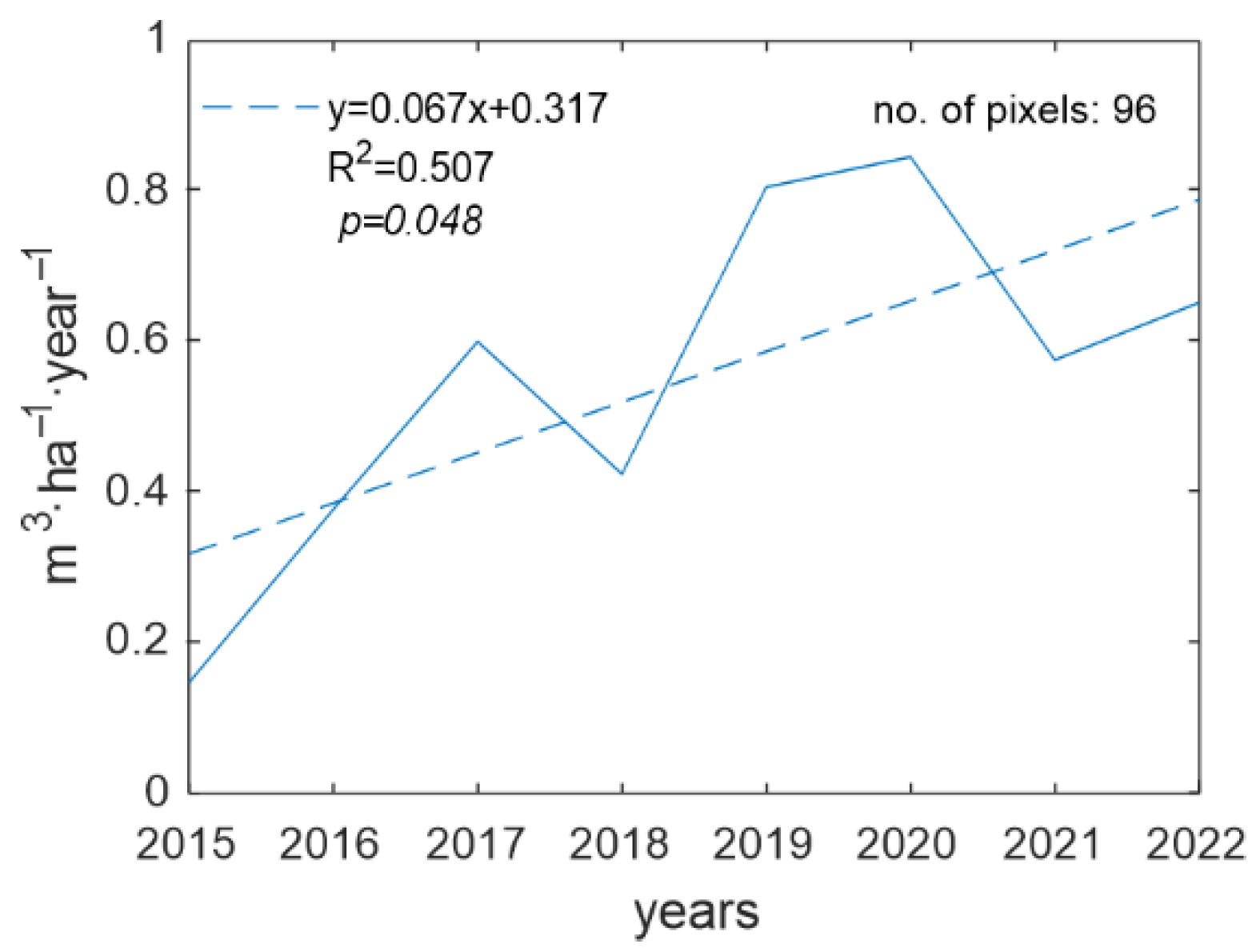
3.2. Temporal Variations in the Volume of Dead Trees

The volume of dead trees removed during sanitation felling, as the effect of forest disturbance, was different in individual years and regions. Out of the three regional directorates of the state forest, the largest number of dead trees was collected in lowlands, uplands, and mountains of the most western region—Wroclaw—making it the ecosystem most vulnerable to disturbances (Figure 5a). The total volume of dead trees in Wroclaw region exceeded 247,000 m3 in 2015, 1,071,000 m3 in 2019, and 317,000 m3 in 2022, and was allocated mostly to pine and spruce (Figure 5a,b and Figure 6a,d,g). In the Lodz and Lublin regions, the volume of dead trees was substantially smaller, with a maximum volume of 118,000 m3 gathered in 2019 in Lodz and 288,000 m3 gathered in 2018 in Lublin (Figure 5a).
The largest part of the dead trees removed in all years originated from pine and spruce (Figure 5b). Two peaks in the volume of dead trees gathered from spruce were in 2016 and 2019 (685,000 m3, and 771,000 m3, respectively), while the maximum volumes gathered from pine were lower and reached 348,000 m3 in 2016 and 510,000 m3 in 2020 (Figure 5b). Oak’s maximum dead trees’ volume exceeded 89,000 m3 in 2020, and beeches reached only 8000 m3 in 2017 and 2019 (Figure 5b).

3.3. Coupling the Trends in NDVI and EVI Z-Scores with the Course of Dead Trees

In order to determine which of the spectral indicators best reflects the actual forest condition, the coupling of the detected trends in NDVI and EVI z-scores with the course of the volume of dead trees was applied. The basis for this analysis is the assumption that when the condition of forest increases, the volume of the removed dead trees should decrease. Hence, a positive trend in the spectral index values should be reflected by a negative trend in the volume of dead trees, and vice versa.
Concerning NDVI z-scores, in the mask of all-species and in all three directorates, the mean (i.e., spatially averaged) volume of dead trees during the analysed period was slightly decreasing in the ‘strong positive’ trend class, while the mean volumes of dead trees in the ‘moderate negative’ and ‘strong negative’ classes were gradually increasing (Figure 7a). The slopes for the trend in changes in the mean volume of dead trees in ‘strong positive’ and ‘strong negative’ classes were statistically significant and amounted to −0.019 and 0.064, respectively (Table 3). This pattern was visible clearly in Wroclaw region, where both ‘strong negative’ and ‘moderate negative’ trend classes showed significant positive trends in the mean volume of dead trees (Figure 7c, Table 3). Simultaneously, both ‘strong positive’ and ‘moderate positive’ trend classes presented a negative trend in the mean volume of dead trees. In Lodz region, statistically significant increasing trends in the mean volume of dead trees occurred in both ‘negative’ trend classes (Figure 7e, Table 3). On the contrary, in Lublin region, there was a statistically significant decrease in the mean volume of dead trees, which occurred in the ‘strong positive’ trend class—with a slope of −0.026 (Figure 7g, Table 3).
On the other hand, the results obtained for EVI z-scores trend class masks are contrasted with those obtained for NDVI z-scores. In the mask of the all-species and in all three directorates, an increase in the mean volume of dead trees was present not only in both ‘negative’ trend classes but also in both ‘positive’ trend classes (Figure 7b, Table 3). This is also the case in Wroclaw and the Lodz region, with the latter having not only statistically significant positive trends in the mean volume of dead trees in both ‘negative’ trend classes (slopes 0.061 and 0.092, for ‘strong negative’ and ‘moderate negative’, respectively) but also in the ‘moderate positive’ trend class (slope 0.036) (Figure 7d,f, Table 3). Instead, the Lublin region was characterised by indifferent trends in the mean volume of dead trees (Figure 7h).
In order to make the research results more comprehensive, the coupling of the detected trends in NDVI and EVI z-scores with the course of the volume of dead trees was additionally applied to the pixels contained within all the directorates but within the masks representing individual tree species. Regarding NDVI z-scores, pine showed a significant increase in the mean volume of dead trees in the ‘strong negative’ trend class (0.043) and a significant decrease in the mean volume of dead trees in the ‘strong positive’ trend class (−0.015) (Figure 8a, Table 3). Contrary to that, for EVI z-scores, all the trend classes presented a slight increase in the mean volume of dead trees in the pine mask (Figure 8b, Table 3). Spruce, which grows mostly in the Wroclaw region, in the analysed period, presented strongly and significantly increasing values of the mean volume of dead trees in the ‘strong negative’ and ‘moderate negative’ trend classes in NDVI z-scores. These increasing slopes (0.221 and 0.118, respectively) were twice as large, as the corresponding slopes in the trend class masks in EVI z-scores (0.104 and 0.053, respectively) (Figure 8c,d, Table 3). At the same time, the ‘positive’ trend classes in the spruce mask showed a gradual decrease in the mean volume of dead trees in NDVI z-scores and an increase in EVI z-scores. Concerning oak, positive trends in the mean volume of dead trees occurred in both ‘negative’ trend class masks, both in NDVI and EVI z-scores. A positive and significant trend in the mean volume of dead trees was also visible in the ‘moderate positive’ trend class mask in EVI z-scores (slope 0.149) (Figure 8f, Table 3), while in NDVI z-scores, the trends in changes in the mean volume of dead trees in the ‘positive’ trend class masks were rather indifferent. When it comes to the last analysed species, beech, it should be borne in mind that the actual number of pixels, out of which the mean volume of dead trees in a given year was averaged, is quite low, especially in the ‘negative’ trend class masks. Therefore, the courses of dead trees in these trend classes are prone to vagueness, and the resulting slopes for the linear trends might be uncertain. Yet, in the ‘overall positive’ trend class mask (i.e., ‘moderate positive’ and ‘strong positive’ trend classes together) within the beech mask, the mean volume of dead trees in the analysed period was gradually decreasing, both regarding the NDVI and EVI z-scores (slopes −0.145 and −0.164, respectively) (Figure 8g,h, Table 3).
At this point it should be mentioned that the linear trends in changes in the volume of dead trees are calculated on the basis of eight values only (one averaged value of the volume of dead trees per each year). Because the time series is short, not many slopes in Table 3 are statistically significant, even if they seem to be substantial. Yet, apart from the statistical significance of the detected slopes, their direction can be also considered as a proper parameter in deciding which of the spectral indicators reflects better the ‘ground truth’. Based on the assumption that an increase (decrease) in the forest condition should be reflected by a decrease (increase) in the volume of removed dead trees, we may say that the positive trend in the spectral index values is ‘in agreement’ with the negative trend in the volume of dead trees. Consequently, in eight analysed cases (all-species, pine, spruce, oak, beech, all-species Wroclaw, all-species Lodz, all-species Lublin), considering the results based on the NDVI masks z-score, six out of eight slopes were in agreement in the ‘overall positive’ trend class, with the same number for the ‘overall negative’ trend class (Table 3). This is a substantially larger number than in the case of the results based on EVI masks z-scores, where only two out of eight slopes were in agreement in the ‘overall positive’ trend class, and seven slopes were in agreement in the ‘overall negative’ trend class.
In general, as previously said, during the period 2015–2022, NDVI z-scores reported more pixels with a significant negative trend of vegetation condition than EVI z-scores (cf. Figure 4). This means that there are MODIS grid cells, which have a significant negative slope for the trend in changes in NDVI z-scores, but it changes into a significant positive slope in EVI z-scores. The course of the mean volume of dead trees in such pixels was also calculated and is presented in Figure 9. A statistically significant (α = 0.05) and positive trend in the mean volume of dead trees was fitted to this course, with a slope of 0.067 and coefficient of determination value of 0.507. Preparing a similar figure, but the other way round (meaning from the pixels with a significant negative slope for the trend in changes in EVI z-scores and a significant positive slope in NDVI z-scores) was not possible, due to the lack of such pixels.

4. Discussion

In this study, during the long period 2002–2022, a generally increasing trend of 0.004 of the NDVI z-score per month was revealed. This reflects an approximately 0.02 NDVI increase in the whole analysed 21-year period. A similar NDVI increase (from 0.009 to 0.030) was indicated for all forests in Poland, in the period 2002–2021 [12]. However, researchers note that the increase in vegetation indices is not stable over time [45,47,48], with a significant turning point, stopping the intensive greening, in 2015 [45]. In 2015, an intense and spatially extended drought affected Europe, including especially its eastern part [49], causing a reduction in the growth rate of many tree species. Indeed, a negative trend in changes in spatially averaged NDVI z-scores occurred in years 2015–2022 in our study area, while the trend in EVI z-scores was, surprisingly, still positive. Analysing the spatial distribution of the slopes for the trend in changes in NDVI and EVI z-scores in all directorates of the state forest, it seems that EVI overestimates the number of positive slopes.
After 2015, subsequent severe droughts occurred in Europe in 2018 [5,50] and 2019 [50,51], with huge impact on the study area [52]. Drought’s impact on forest conditions is highlighted in many studies [5,53]. It can deteriorate tree health, leading to large-scale die-offs, with consequences for biodiversity, the carbon cycle, and wood production [54]. As the forest’s response to a severe meteorological condition might be substantially lagged [55,56], the maximum volume of dead trees removed during sanitation felling occurred in 2019 (for spruce) and 2020 (for pine). However, drought is not the only factor influencing the dead trees’ volume. Natural disturbances, such as wildfires, wind, snow, and insects, can have a significant impact on the dead trees’ dynamics [30,57,58]. Yet, apart from pests, other factors were not included in this analysis (we used only the volume of dead trees related to pest/drought). In addition, characteristics of the forest stand, e.g., stand age, height, height growth rate, and site productivity, were found to influence the dead trees’ volume [34,35,59].
This study reports the linear trends in changes in the volume of dead trees, obtained within the individual trend class masks, prepared on the basis of NDVI and EVI z-scores. When negative trend class masks are examined, both NDVI and EVI z-scores give similar results, i.e., in the pixels with a decreasing trend in both spectral indicators’ values, the course of dead trees was similar (significantly increasing). However, the course of dead trees was mostly decreasing in those places, where NDVI z-scores give positive trends, making NDVI and dead trees consistent. The reverse holds true for EVI z-scores: in places where EVI z-scores give positive trends, the course of dead trees was, in many cases, also positive, making the EVI and dead trees rather inconsistent. The cause may lie in an excessive number of pixels with a significant positive trend in EVI z-scores. The fact that the course of the mean volume of dead trees is significantly increasing in solely those pixels, which hold positive trend in z-scores EVI but negative in z-scores NDVI might serve here as an additional confirmation.
Indeed, NDVI seems to reflect best the condition of forest vegetation in the whole analysed study area. This statement is also valid in relation to the Wroclaw region only and to the specific species, pine and spruce. According to recent research results, NDVI is more effective than EVI in monitoring pine growth patterns in other places, e.g., in southern Brazil [60]. NDVI was considered as a better predictor of the natural forest vegetation in the temperate zone in China [24], although this work correlated values from the MODIS NDVI and EVI with ground measurements of vegetation in the growing season of only one year, thus lacking temporal variation, which is a very important component in environmental studies. NDVI- and EVI-based machine learning models were also used to forecast vegetation for 2019 by [61], giving an error of 1.51–5.73% for NDVI and 4.33–6.99% for EVI. Researchers suggest that NDVI works well when the spectral reflectance in both near-infrared and red bands deteriorates together, while its performance decreases when the spectral reflectance in these bands varies substantially [60]. EVI, on the other hand, has been found to be effective in monitoring tree growth patterns until a certain age, after which it may become saturated, indicating a decline in its effectiveness, compared to NDVI [60]. The research undertaken in this paper did not distinguish trees by age, but the introduction of such a variable (forest stand age) could be of interest in future research. Another important factor influencing the performance of NDVI and EVI is the topographic effect. The evaluation based on two criteria: the correlation with a local illumination condition and the dependence on an aspect, showed that the topographic effect can be neglected for NDVI, while it heavily influences EVI, with 25.37% of its variation explained by the local illumination condition [62]. This could partially explain the relatively good results of the NDVI z-scores in the pixels occupied by spruce, located in the mountain at the southern edges of the Wroclaw region. Finally, although NDVI is sensitive to atmospheric influence [6] and saturates at a high level of biomass [9,10], this seems not to affect the good results obtained, especially for coniferous species, which usually have lower levels of biomass than broadleaved species. Hence, NDVI is a good predictor of forest vegetation in the European temperate zone.
The study has, however, some limitations. The first might be the use of dead trees. Although it is considered as a crucial indicator of forest disturbance [33], the volume of dead trees is neither the only nor the most precise vegetation indicator, and analyses based on it are approximate and must be treated with caution. In addition, MODIS’s 250 m pixels may include signals not only from the canopy layer but also from the understorey and non-forest ground, obscuring the signals of small-patch sanitation felling. This might result in an underrepresentation of the localised canopy loss. However, a relatively large number of pixels used in this study, from which the statistics were calculated, reduces the level of uncertainty of the research results. Another important issue is the fact that the linear trends in changes in the volume of dead trees were calculated on the basis of eight yearly values only. Previous studies have shown that the temporal response of the spectral indices to tree mortality events may lag by several years [63]. Climate-induced tree-mortality pulses can be obscured by broad-scale and long-term greening [63]; so, it takes many more years to fully characterise the forest condition in a given place. This raises the need for further research on this topic in the future, based on increasingly longer measurement data series.

5. Conclusions

The results presented in this paper show in detail the coupling of the MODIS-based NDVI and EVI data with the data on the volume of dead trees removed during sanitation felling in the three regional directorates of state forest in Poland, during the period 2015–2022. We identified the classes of the trend in changes in NDVI and EVI z-scores in forests of the European temperate zone and spatiotemporal variations in the dead trees’ volume. In order to assess which satellite-borne index best represents the actual forest condition, the trends in changes in NDVI and EVI z-scores were compared with the respective trends in the volume of dead trees, following the assumption that a positive trend in the spectral index values should be reflected by a negative trend in the volume of dead trees, and vice versa. The analyses were carried out for the pixels within the all-species mask in the study area and for the pixels representing the individual tree species.
In general, NDVI is a good predictor of the forest vegetation in the European temperate zone and substantially better than EVI. Spatially, NDVI gives more pixels with a negative slope for the trend in changes in spectral index values than EVI, while EVI seems to overestimate the number of positive slopes. The larger number of negative slopes in the trend in changes in NDVI z-scores applies mostly to the Wroclaw region and seems to be in agreement with the increasing volume of dead trees in the analysed period.
Comparing the detected trend class masks for spectral indices and the multi-annual course of dead trees, in 12 out of 16 cases, the slopes of the trend in changes in NDVI z-scores were in agreement with the slopes of the trend in the volume of dead trees, while for EVI, this number was reduced to 9. Moreover, NDVI reflects substantially better the condition of coniferous forest in pine and spruce masks, which constitute 87.0% of the analysed pixels.
This paper enhances knowledge in the area of the performance of NDVI and EVI, in relation to monitoring selected forest tree species in the European temperate zone. As NDVI and EVI are spectral indicators for vegetation conditions, widely used by researchers worldwide, the results of this work fill the knowledge gap on the suitability of using them in relation to forest vegetation in the European temperate zone.

Author Contributions

K.K.: Conceptualisation, Methodology, Formal analysis, Investigation, Data Curation, Writing—Original Draft, Writing—Review and Editing, Visualisation. P.H.: Data Curation, Writing—Review and Editing. J.S.: Writing—Review and Editing, Funding acquisition. A.H.: Conceptualization, Writing—Review and Editing, Supervision, Project administration, Funding acquisition. All authors have read and agreed to the published version of the manuscript.

Funding

This work was supported by the National Science Centre in Poland [grant number 2021/41/B/ST10/04113].

Data Availability Statement

Data on NDVI and EVI are publicly available in the NASA EOSDIS Land Processes Distributed Active Archive Center (http://search.earthdata.nasa.gov). Data on the volume of dead trees are confidential.

Conflicts of Interest

The authors declare no conflicts of interest.

References

  1. FAO; UNEP. The State of the World’s Forests 2020. In Forests, Biodiversity and People; FAO and UNEP: Rome, Italy, 2020. [Google Scholar] [CrossRef]
  2. Pan, Y.; Birdsey, R.A.; Phillips, O.L.; Jackson, R.B. The Structure, Distribution, and Biomass of the World’s Forests. Annu. Rev. Ecol. Evol. Syst. 2013, 44, 593–622. [Google Scholar] [CrossRef]
  3. de Rigo, D.; Bosco, C.; San-Miguel-Ayanz, J.; Houston Durrant, T.; Barredo, J.I.; Strona, G.; Caudullo, G.; Di Leo, M.; Boca, R. Forest resources in Europe: An overview on ecosystem services, disturbances and threats. In European Atlas of Forest Tree Species; San-Miguel-Ayanz, J., de Rigo, D., Caudullo, G., Houston Durrant, T., Mauri, A., Eds.; Publications Office of the EU: Luxembourg, 2016; p. e015b050. [Google Scholar]
  4. Adole, T.; Dash, J.; Atkinson, P.M. A systematic review of vegetation phenology in Africa. Ecol. Inform. 2016, 34, 117–128. [Google Scholar] [CrossRef]
  5. Buras, A.; Rammig, A.; Zang, C.S. Quantifying impacts of the 2018 drought on European ecosystems in comparison to 2003. Biogeosciences 2020, 17, 1655–1672. [Google Scholar] [CrossRef]
  6. Huang, S.; Tang, L.; Hupy, J.P.; Wang, Y.; Shao, G. A commentary review on the use of Normalized Difference Vegetation Index (NDVI) in the era of popular remote sensing. J. For. Res. 2021, 32, 1–6. [Google Scholar] [CrossRef]
  7. Soubry, I.; Doan, T.; Chu, T.; Guo, X. A Systematic Review on the Integration of Remote Sensing and GIS to Forest and Grassland Ecosystem Health Attributes, Indicators, and Measures. Remote Sens. 2021, 13, 3262. [Google Scholar] [CrossRef]
  8. Didan, K.; Munoz, A.B. MODIS Vegetation Index User’s Guide (MOD13 Series); Vegetation Index and Phenology Lab, The University of Arizona: Tucson, AZ, USA, 2019. [Google Scholar]
  9. Gao, X.; Huete, A.R.; Ni, W.; Miura, T. Optical–Biophysical Relationships of Vegetation Spectra without Background Contamination. Remote Sens. Environ. 2000, 74, 609–620. [Google Scholar] [CrossRef]
  10. Van Der Meer, F.; Bakker, W.; Scholte, K.; Skidmore, A.; De Jong, S.; Clevers, J.; Addink, E.; Epema, G. Spatial scale variations in vegetation indices and above-ground biomass estimates: Implications for MERIS. Int. J. Remote Sens. 2001, 22, 3381–3396. [Google Scholar] [CrossRef]
  11. Huete, A.; Didan, K.; Miura, T.; Rodriguez, E.P.; Gao, X.; Ferreira, L.G. Overview of the radiometric and biophysical performance of the MODIS vegetation indices. Remote Sens. Environ. 2002, 83, 195–213. [Google Scholar] [CrossRef]
  12. Kulesza, K.; Hościło, A. Influence of climatic conditions on Normalized Difference Vegetation Index variability in forest in Poland (2002–2021). Meteorol. Appl. 2023, 30, e2156. [Google Scholar] [CrossRef]
  13. Barka, I.; Bucha, T.; Molnár, T.; Móricz, N.; Somogyi, Z.; Koreň, M. Suitability of MODIS-based NDVI index for forest monitoring and its seasonal applications in Central Europe. Cent. Eur. For. J. 2019, 65, 206–217. [Google Scholar] [CrossRef]
  14. Prăvălie, R.; Sîrodoev, I.; Nita, I.-A.; Patriche, C.; Dumitraşcu, M.; Roşca, B.; Tişcovschi, A.; Bandoc, G.; Săvulescu, I.; Mănoiu, V.; et al. NDVI-based ecological dynamics of forest vegetation and its relationship to climate change in Romania during 1987–2018. Ecol. Indic. 2022, 136, 108629. [Google Scholar] [CrossRef]
  15. Yang, Y.; Wang, S.; Bai, X.; Tan, Q.; Li, Q.; Wu, L.; Tian, S.; Hu, Z.; Li, C.; Deng, Y. Factors Affecting Long-Term Trends in Global NDVI. Forests 2019, 10, 372. [Google Scholar] [CrossRef]
  16. Gazol, A.; Camarero, J.J.; Vicente-Serrano, S.M.; Sánchez-Salguero, R.; Gutiérrez, E.; de Luis, M.; Sangüesa-Barreda, G.; Novak, K.; Rozas, V.; Tíscar, P.A.; et al. Forest resilience to drought varies across biomes. Glob. Change Biol. 2018, 24, 2143–2158. [Google Scholar] [CrossRef] [PubMed]
  17. Araghi, A.; Martinez, C.J.; Adamowski, J.; Olesen, J.E. Associations between large-scale climate oscillations and land surface phenology in Iran. Agric. For. Meteorol. 2019, 278, 107682. [Google Scholar] [CrossRef]
  18. Farbo, A.; Sarvia, F.; De Petris, S.; Basile, V.; Borgogno-Mondino, E. Forecasting corn NDVI through AI-based approaches using sentinel 2 image time series. ISPRS J. Photogramm. Remote Sens. 2024, 211, 244–261. [Google Scholar] [CrossRef]
  19. Moreira, A.; Fontana, D.C.; Kuplich, T.M. Wavelet approach applied to EVI/MODIS time series and meteorological data. ISPRS J. Photogramm. Remote Sens. 2019, 147, 335–344. [Google Scholar] [CrossRef]
  20. Tang, W.X.; Liu, S.G.; Kang, P.; Peng, X.; Li, Y.Y.; Guo, R.; Jia, J.N.; Liu, M.C.; Zhu, L.J. Quantifying the lagged effects of climate factors on vegetation growth in 32 major cities of China. Ecol. Indic. 2021, 132, 108290. [Google Scholar] [CrossRef]
  21. Galvao, L.S.; dos Santos, J.R.; Roberts, D.A.; Breunig, F.M.; Toomey, M.; de Moura, Y.M. On intra-annual EVI variability in the dry season of tropical forest: A case study with MODIS and hyperspectral data. Remote Sens. Environ. 2011, 115, 2350–2359. [Google Scholar] [CrossRef]
  22. Lara, C.; Saldías, G.S.; Cazelles, B.; Rivadeneira, M.M.; Muñoz, R.; Galán, A.; Paredes, A.L.; Fierro, P.; Broitman, B.R. Climatic Regulation of Vegetation Phenology in Protected Areas along Western South America. Remote Sens. 2021, 13, 2590. [Google Scholar] [CrossRef]
  23. Zhang, Y.; Song, C.; Band, L.E.; Sun, G.; Li, J. Reanalysis of global terrestrial vegetation trends from MODIS products: Browning or greening? Remote Sens. Environ. 2017, 191, 145–155. [Google Scholar] [CrossRef]
  24. Li, Z.; Li, X.; Wei, D.; Xu, X.; Wang, H. An assessment of correlation on MODIS-NDVI and EVI with natural vegetation coverage in Northern Hebei Province, China. Procedia Environ. Sci. 2010, 2, 964–969. [Google Scholar] [CrossRef]
  25. Miura, T.; Smith, C.Z.; Yoshioka, H. Validation and analysis of Terra and Aqua MODIS, and SNPP VIIRS vegetation indices under zero vegetation conditions: A case study using Railroad Valley Playa. Remote Sens. Environ. 2021, 257, 112344. [Google Scholar] [CrossRef]
  26. Khare, S.; Deslauriers, A.; Morin, H.; Latifi, H.; Rossi, S. Comparing Time-Lapse PhenoCams with Satellite Observations across the Boreal Forest of Quebec, Canada. Remote Sens. 2022, 14, 100. [Google Scholar] [CrossRef]
  27. Crespo-Antia, J.P.; Gazol, A.; Pizarro, M.; de Andrés, E.G.; Valeriano, C.; Cuadrado, A.R.; Linares, J.C.; Camarero, J.J. Matching Vegetation Indices and Tree Vigor in Pyrenean Silver Fir Stands. Remote Sens. 2024, 16, 4564. [Google Scholar] [CrossRef]
  28. Aubard, V.; Paulo, J.A.; Silva, J.M.N. Long-Term Monitoring of Cork and Holm Oak Stands Productivity in Portugal with Landsat Imagery. Remote Sens. 2019, 11, 525. [Google Scholar] [CrossRef]
  29. Sinan, M.; Hasenauer, H. How to determine the leaf area index (LAI) of forests: A comparison of forest inventory versus satellite-driven estimates. For. Ecosyst. 2025, 13, 100332. [Google Scholar] [CrossRef]
  30. Čuchta, P. Natural disturbances (with a special reference to windthrow): A literature review. In Advances in Environmental Research; Nova: New York, NY, USA, 2020; Volume 72, pp. 153–172. [Google Scholar]
  31. Đuka, A.; Franjević, M.; Tomljanović, K.; Popović, M.; Ugarković, D.; Teslak, K.; Barčić, D.; Žagar, K.; Palatinuš, K.; Papa, I. A Decade of Sanitary Fellings Followed by Climate Extremes in Croatian Managed Forests. Land 2025, 14, 766. [Google Scholar] [CrossRef]
  32. Lech, P.; Kamińska, A. “Mortality, or not mortality, that is the question …”: How to Treat Removals in Tree Survival Analysis of Central European Managed Forests. Plants 2024, 13, 248. [Google Scholar] [CrossRef] [PubMed]
  33. Shvidenko, A.; Mukhortova, L.; Kapitsa, E.; Kraxner, F.; See, L.; Pyzhev, A.; Gordeev, R.; Fedorov, S.; Korotkov, V.; Bartalev, S.; et al. A Modelling System for Dead Wood Assessment in the Forests of Northern Eurasia. Forests 2023, 14, 45. [Google Scholar] [CrossRef]
  34. Socha, J.; Hawryło, P.; Tymińska-Czabańska, L.; Reineking, B.; Lindner, M.; Netzel, P.; Grabska-Szwagrzyk, E.; Vallejos, R.; Reyer, C.P.O. Higher site productivity and stand age enhance forest susceptibility to drought-induced mortality. Agric. For. Meteorol. 2023, 341, 109680. [Google Scholar] [CrossRef]
  35. Tymińska-Czabańska, L.; Hawryło, P.; Janiec, P.; Socha, J. Tree height, growth rate and stand density determined by ALS drive probability of Scots pine mortality. Ecol. Indic. 2022, 145, 109643. [Google Scholar] [CrossRef]
  36. Tomczyk, A.M.; Bednorz, E. Atlas Klimatu Polski (1991–2020); Bogucki Wydawnictwo Naukowe: Poznan, Poland, 2022. [Google Scholar]
  37. Zajączkowski, G.; Jabłołski, M.; Jabłołski, T.; Sikora, K.; Kowalska, A.; Małachowska, J.; Piwnicki, J. (Eds.) Raport o Stanie Lasów w Polsce 2021; Centrum Informacyjne Lasów Państwowych: Warsaw, Poland, 2022. [Google Scholar]
  38. RDLP Lublin. Lasy Regionu. Available online: https://www.lublin.lasy.gov.pl/lasy-regionu (accessed on 14 December 2023).
  39. Zięba, M. Lasy Regionu. Available online: https://www.wroclaw.lasy.gov.pl/lasy-regionu (accessed on 14 December 2023).
  40. Hościło, A.; Lewandowska, A. Mapping Forest Type and Tree Species on a Regional Scale Using Multi-Temporal Sentinel-2 Data. Remote Sens. 2019, 11, 929. [Google Scholar] [CrossRef]
  41. Hościło, A.; Kulesza, K.; Lewandowska, A. Application of Sentinel-2 Data for Mapping Tree Species and Detecting Forest Decline. In Proceedings of the CLMS General Assembly 2025, Cracow, Poland, 20–22 May 2025; Available online: https://clms-general-assembly-global-network-users.mailerpage.io/posters-2025 (accessed on 15 June 2025).
  42. Didan, K. MODIS/Aqua Vegetation Indices 16-Day L3 Global 250m SIN Grid V061 [Data Set]; NASA EOSDIS Land Processes DAAC: Pasadena, CA, USA, 2021. [Google Scholar] [CrossRef]
  43. Didan, K. MODIS/Terra Vegetation Indices 16-Day L3 Global 250m SIN Grid V061 [Data Set]; NASA EOSDIS Land Processes DAAC: Pasadena, CA, USA, 2021. [Google Scholar] [CrossRef]
  44. Holben, B.N. Characteristics of maximum-value composite images from temporal AVHRR data. Int. J. Remote Sens. 1986, 7, 1417–1434. [Google Scholar] [CrossRef]
  45. Kulesza, K.; Hościło, A. Temporal Patterns of Vegetation Greenness for the Main Forest-Forming Tree Species in the European Temperate Zone. Remote Sens. 2024, 16, 2844. [Google Scholar] [CrossRef]
  46. FDB Polish Forest Data Bank. Polish State Forests State Holding; 2024. Available online: https://www.bdl.lasy.gov.pl/portal/en (accessed on 14 December 2024).
  47. Liu, Y.; Li, Y.; Li, S.; Motesharrei, S. Spatial and Temporal Patterns of Global NDVI Trends: Correlations with Climate and Human Factors. Remote Sens. 2015, 7, 13233–13250. [Google Scholar] [CrossRef]
  48. Piao, S.; Wang, X.; Ciais, P.; Zhu, B.; Wang, T.; Liu, J. Changes in satellite-derived vegetation growth trend in temperate and boreal Eurasia from 1982 to 2006. Glob. Change Biol. 2011, 17, 3228–3239. [Google Scholar] [CrossRef]
  49. Ionita, M.; Tallaksen, L.M.; Kingston, D.G.; Stagge, J.H.; Laaha, G.; Van Lanen, H.A.J.; Scholz, P.; Chelcea, S.M.; Haslinger, K. The European 2015 drought from a climatological perspective. Hydrol. Earth Syst. Sci. 2017, 21, 1397–1419. [Google Scholar] [CrossRef]
  50. Boergens, E.; Güntner, A.; Dobslaw, H.; Dahle, C. Quantifying the Central European Droughts in 2018 and 2019 With GRACE Follow-On. Geophys. Res. Lett. 2020, 47, e2020GL087285. [Google Scholar] [CrossRef]
  51. Hari, V.; Rakovec, O.; Markonis, Y.; Hanel, M.; Kumar, R. Increased future occurrences of the exceptional 2018–2019 Central European drought under global warming. Sci. Rep. 2020, 10, 12207. [Google Scholar] [CrossRef] [PubMed]
  52. Somorowska, U. Amplified signals of soil moisture and evaporative stresses across Poland in the twenty-first century. Sci. Total Environ. 2022, 812, 151465. [Google Scholar] [CrossRef] [PubMed]
  53. Schuldt, B.; Buras, A.; Arend, M.; Vitasse, Y.; Beierkuhnlein, C.; Damm, A.; Gharun, M.; Grams, T.E.E.; Hauck, M.; Hajek, P.; et al. A first assessment of the impact of the extreme 2018 summer drought on Central European forests. Basic Appl. Ecol. 2020, 45, 86–103. [Google Scholar] [CrossRef]
  54. Brun, P.; Psomas, A.; Ginzler, C.; Thuiller, W.; Zappa, M.; Zimmermann, N.E. Large-scale early-wilting response of Central European forests to the 2018 extreme drought. Glob. Change Biol. 2020, 26, 7021–7035. [Google Scholar] [CrossRef] [PubMed]
  55. Carl, G.; Doktor, D.; Koslowsky, D.; Kühn, I. Phase difference analysis of temperature and vegetation phenology for beech forest: A wavelet approach. Stoch. Environ. Res. Risk Assess. 2013, 27, 1221–1230. [Google Scholar] [CrossRef]
  56. Kulesza, K.; Hościło, A. Coherency and time lag analyses between MODIS vegetation indices and climate across forests and grasslands in the European temperate zone. Biogeosciences 2024, 21, 2509–2527. [Google Scholar] [CrossRef]
  57. Dossa, G.G.O.; Paudel, E.; Schaefer, D.; Zhang, J.L.; Cao, K.F.; Xu, J.C.; Harrison, R.D. Quantifying the factors affecting wood decomposition across a tropical forest disturbance gradient. For. Ecol. Manag. 2020, 468, 118166. [Google Scholar] [CrossRef]
  58. Burton, J.E.; Bennett, L.T.; Kasel, S.; Nitschke, C.R.; Tanase, M.A.; Fairman, T.A.; Parker, L.; Fedrigo, M.; Aponte, C. Fire, drought and productivity as drivers of dead wood biomass in eucalypt forests of south-eastern Australia. For. Ecol. Manag. 2021, 482, 118859. [Google Scholar] [CrossRef]
  59. Vlad, R.; Sidor, C.G.; Dinca, L.; Constandache, C.; Grigoroaea, D.A.N.; Ispravnic, A.; Pei, G. Dead wood diversity in a Norway spruce forest from the cãlimani national park (The eastern carpathians). Balt. For. 2019, 25, 238–248. [Google Scholar] [CrossRef]
  60. Käfer, P.S.; Rex, F.E.; Breunig, F.M.; Balbinot, R. Modeling pinus elliottii growth with multitemporal landsat data: A study case in southern Brazil. Bol. Cienc. Geod. 2018, 24, 286–299. [Google Scholar] [CrossRef]
  61. Roy, B. Optimum machine learning algorithm selection for forecasting vegetation indices: MODIS NDVI & EVI. Remote Sens. Appl. Soc. Environ. 2021, 23, 100582. [Google Scholar] [CrossRef]
  62. Chen, R.; Yin, G.; Liu, G.; Li, J.; Verger, A. Evaluation and normalization of topographic effects on vegetation indices. Remote Sens. 2020, 12, 2290. [Google Scholar] [CrossRef]
  63. Yan, Y.; Piao, S.; Hammond, W.M.; Chen, A.; Hong, S.; Xu, H.; Munson, S.M.; Myneni, R.B.; Allen, C.D. Climate-induced tree-mortality pulses are obscured by broad-scale and long-term greening. Nat. Ecol. Evol. 2024, 8, 912–923. [Google Scholar] [CrossRef] [PubMed]
Figure 1. The location of the regional directorates of state forest used in this study (1—Wroclaw, 2—Lodz, 3—Lublin) and the spatial distribution of six tree species masks in MODIS grid (pine, oak, beech, spruce, birch, and alder).
Remotesensing 17 02549 g001
Figure 2. Flow chart of the input data and the methodology used in this study.
Remotesensing 17 02549 g002
Figure 3. The course of the spatially averaged NDVI z-scores (a) and EVI z-scores (b) during the longer period 2002–2022. The graph presents also the linear trends in the longer period 2002–2022 and basic period 2015–2022 (coloured dashed lines are explained next to the graph), together with the trend line equations, the coefficients of determination R2, and the p-values.
Remotesensing 17 02549 g003
Figure 4. The slopes for the trend in changes in NDVI z-scores (NDVI z-score month−1, upper panel) and EVI z-scores (EVI z-score·month−1, lower panel) in the all-species mask in the three regional directorates of the state forest: Wroclaw (a,d), Lodz (b,e), and Lublin (c,f), during the period 2015–2022. The values of the trend’s slopes are divided into five classes, according to their statistical significance at the significance level of α = 0.05 and the slope’s steepness (one insignificant and four significant classes).
Remotesensing 17 02549 g004
Figure 5. The total volume of dead trees (m3·year−1) removed during sanitation felling, during the period 2015–2022: in the individual regional directorates of the state forest (a) and from the individual tree species (b).
Remotesensing 17 02549 g005
Figure 6. The volume of dead trees (m3·ha−1·year−1) in the dead trees mask in the MODIS grid removed during sanitation felling in the regional directorate of the state forest in Wroclaw (a,d,g), Lodz (b,e,h), and Lublin (c,f,i), during 2015, 2019, and 2022.
Remotesensing 17 02549 g006
Figure 7. The mean (spatially averaged) volume of dead trees (m3·ha−1·year−1) removed during sanitation felling in the pixels contained within the intersection of the dead trees mask, the all-species mask, and the individual trend class masks for NDVI z-scores (left column) and EVI z-scores (right column) during the period 2015–2022, in all the regional directorates of the state forest (a,b), in Wroclaw (c,d), in Lodz (e,f), and in Lublin (g,h). The graphs also present the actual numbers of pixels, from which the mean volume of dead trees in each year was calculated.
Remotesensing 17 02549 g007
Figure 8. The mean (spatially averaged) volume of dead trees (m3·ha−1·year−1) removed during sanitation felling in the pixels contained within the intersection of the dead trees mask, the individual species masks—pine (a,b), spruce (c,d), oak (e,f), and beech (g,h)—and the individual trend class masks for NDVI z-scores (left column) and EVI z-scores (right column), during the period 2015–2022. The graphs present also the actual numbers of pixels out of which the mean volume of dead trees in each year was calculated.
Remotesensing 17 02549 g008
Figure 9. The mean (spatially averaged) volume of dead trees (m3·ha−1·year−1) removed during sanitation felling in the pixels contained within the intersection of the dead trees mask, the all-species mask, both ‘negative’ trend class masks in NDVI z-score and both ‘positive’ trend class masks in EVI z-score, during the period 2015–2022, in the all regional directorates of the state forest. The graph also presents the linear trend, together with the trend line equation, the coefficient of determination R2, and the p-value, as well as the actual number of pixels, from which the mean volume of dead trees in each year was calculated.
Remotesensing 17 02549 g009
Table 1. The number of MODIS pixels in each species mask in the three directorates (Wroclaw, Lodz, and Lublin) and the area (km2) they cover.
Species MaskNumber of MODIS PixelsArea (km2)Used Further in This Study
WroclawLodzLublinTotal
Pine8698968310,23428,6151788.4Yes
Spruce41443944187261.7Yes
Oak40328815922283142.7Yes
Beech3102313971730108.1Yes
Alder9523249181851.1No
Birch10942613.8No
All-species13,66010,27413,76037,6942355.9Yes
Table 2. The percentage of pixels with statistically significant negative, positive, and insignificant trend in changes in NDVI and EVI z-scores during the period 2015–2022, in all the regional directorates of the state forest and in Wroclaw, Lodz, and Lublin separately.
NDVI Z-Score
AreaSignificant negative trends (%)Insignificant trends (%)Significant positive trends (%)
All14.2875.4910.23
Wroclaw28.0369.072.90
Lodz7.4472.0520.52
Lublin5.7384.449.83
EVI Z-Score
AreaSignificant negative trends (%)Insignificant trends (%)Significant positive trends (%)
All3.6173.9322.46
Wroclaw6.9081.7611.35
Lodz2.4960.7636.75
Lublin1.1776.0122.82
Table 3. The slopes for the trend in changes in the mean (spatially averaged) volume of dead trees (m3·ha−1·year−1) removed during sanitation felling in the pixels contained within the intersection of the dead trees mask, the individual species masks, and the individual trend class masks for NDVI z-scores and EVI z-scores during the period 2015–2022. Statistically significant values at the significance level of α = 0.05 (α = 0.1) are in bold (italic).
Trend Class Mask for NDVI Z-Score
Species maskStrong negativeModerate negativeInsignif.Moderate positiveStrong positiveOverall negativeOverall positive
All-species0.0640.0480.0300.002−0.0190.056−0.008
Pine0.0430.0390.0200.007−0.0150.041−0.004
Spruce0.2210.1180.064−0.023−0.0180.169−0.021
Oak0.0500.0410.1000.0060.0160.0440.011
Beech−0.003−0.015−0.054−0.103−0.182−0.011−0.145
All-species, Wroclaw0.0690.0540.057−0.018−0.0180.062−0.018
All-species, Lodz0.0820.0730.0330.011−0.0100.0780.001
All-species, Lublin−0.0020.001−0.004−0.015−0.026−0.001−0.020
Trend Class Mask for EVI Z-Score
Species maskStrong negativeModerate negativeInsignif.Moderate positiveStrong positiveOverall negativeOverall positive
All-species0.0670.0510.0340.0250.0050.0590.015
Pine0.0470.0530.0220.0190.0120.0500.015
Spruce0.1040.0530.0810.0570.0130.0820.040
Oak0.1290.0420.0900.149−0.0110.0950.093
Beech0.020−0.017−0.027−0.117−0.211−0.011−0.164
All-species, Wroclaw0.0750.0530.0590.0430.0250.0640.034
All-species, Lodz0.0610.0920.0370.0360.0040.0760.020
All-species, Lublin0.0030.003−0.005−0.007−0.0080.003−0.008
Disclaimer/Publisher’s Note: The statements, opinions and data contained in all publications are solely those of the individual author(s) and contributor(s) and not of MDPI and/or the editor(s). MDPI and/or the editor(s) disclaim responsibility for any injury to people or property resulting from any ideas, methods, instructions or products referred to in the content.

